The exact $SL(K+3,\mathbb{C})$ symmetry of string theory

Sheng-Hong Lai xgcj944137@gmail.com Department of Electrophysics, National Yang Ming Chiao Tung University, Hsinchu, Taiwan, R.O.C. โ€ƒโ€ƒ Jen-Chi Lee jcclee@cc.nctu.edu.tw Department of Electrophysics, National Yang Ming Chiao Tung University, Hsinchu, Taiwan, R.O.C. Center for Theoretical and Computational Physics (CTCP), National Yang Ming Chiao Tung University, Hsinchu, Taiwan, R.O.C. โ€ƒโ€ƒ Yi Yang yiyang@mail.nctu.edu.tw Department of Electrophysics, National Yang Ming Chiao Tung University, Hsinchu, Taiwan, R.O.C. Center for Theoretical and Computational Physics (CTCP), National Yang Ming Chiao Tung University, Hsinchu, Taiwan, R.O.C.
Abstract

By using on-shell recursion relation of string scattering amplitudes (SSA), we show that all $n$-point SSA of the open bosonic string theory can be expressed in terms of the Lauricella functions. This result extends the previous exact $SL(K+3,\mathbb{C})$ symmetry of the $4$-point Lauricella SSA (LSSA) of three tachyons and one arbitrary string states to the whole tree-level open bosonic string theory. Moreover, we present three applications of the $SL(K+3,\mathbb{C})$ symmetry on the SSA. They are the solvability of all $n$-point SSA in terms of four-tachyon amplitudes, the existence of iteration relations among residues of a given SSA so as to soften its hard scattering behavior and finally the re-derivation of infinite linear relations among hard SSA CHLTY2 .

I Introduction

Symmetry has long been considered as an important property of physical laws for both classical and quantum physics. Historically, symmetry was used to be thought of as one of the direct consequences of equation of motion (EOM) of a physical law before the developments of general relativity and Yang-Mills theory. However, it was soon realized that, in a quantum field theory (QFT) for example, symmetry principle was even more fundamental than the EOM itself. Indeed, it was symmetry which determined the form of the interaction or EOM of a physical law (symmetry dictates interaction). More importantly, for the case of electrodynamics, in contrast to classical physics, only in quantum theory yang can the QED $U(1)$ gauge symmetry be identified and used to derive Ward identities which secure QED as a consistent renormalizable QFT.

In QFT, for example QCD, one usually considers interactions with upย to four-point couplings whose forms are fixed by the symmetry principle. In addition, symmetry principle can be used to derive Slavnov-Taylor identities which relate different couplings. This is in contrast to the four-fermion model in the weak interaction which is not a consistent renormalizable QFT. In string theory, on the contrary, one is given a set of rules through quantum consistency of the extended string which was used to fix the forms of interactions or vertices to calculate perturbative on-shell string scattering amplitudes (SSA). Moreover, instead of up to four-point couplings in QCD, one encounters $n$-point couplings with arbitrary $n$ which correspond to the infinite number of degrees of freedom in the spectrum of string theory. One crucial issue of string theory is thus to identify symmetry of the theory and uses it to relate these infinite number of couplings of particles with arbitrary higher masses and spins.

To identify the exact symmetry group (or even a smaller subgroup) of string theory is much more complicated than that of a QFT. This is because in string theory one needs to deal with infinite number of massive couplings or vertices instead of up to four in a typical QFT. The well-known $E_{8}^{2}$ and $SO(32)$ symmetries of the $10D$ Heterotic string are symmetries of Yang-Mills couplings in the massless sector only. In a series of recent papers, the present authors calculated a subset of exact $4$-point SSA, namely, amplitudes of three tachyons and one arbitrary string states, and expressed them in terms of the $D$-type Lauricella functions LLY2 . In addition, it was shown that these Lauricella SSA (LSSA) can be expressed in terms of the basis functions in the infinite dimensional representation of the $SL(K+3,C)$ group Group . It is important to note that instead of finite dimensional representation of a compact Lie group, here we encounter an infinite dimensional representation of a noncompact Lie group. For any fixed positive integer $K$, we have infinite number of LSSA in the $SL(K+3,C)$ representations slkc . Moreover, it was further shown that there existed $K+2$ recurrence relations among the $D$-type Lauricella functions. These recurrence relations can be used to reproduce the Cartan subalgebra and simple root system of the $SL(K+3,C)$ group with rank $K+2$. As a result, the $SL(K+3,C)$ group with its corresponding stringy Ward identities (recurrence relations) can be used to solve solve all the LSSA and express them in terms of one amplitude. See the recent review paper LSSA .

As an important application of this solvability in the hard string scattering limit, the $SL(K+3,C)$ symmetry group of the LSSA can be used to reproduce LLY2 infinite linear relations with constant coefficients among all hard SSA and solve the ratios among them. These high energy behaviors of string theory GM ; GM1 were first conjectured by Gross Gross and later corrected and proved ChanLee ; ChanLee2 ; CHLTY2 ; CHLTY1 by the method of decoupling of zero norm states (ZNS) Lee ; lee-Ov ; LeePRL . See the review papers review ; over . Since the decoupling of ZNS and thus the infinite linear relations in the hard scattering regime persist to all string loop orders, we conjecture that the $SL(K+3,C)$ symmetry at string-tree level proposed in this letter is also valid for string loop amplitudes. One early attempt using the so-called bracket relations to identify stringy symmetries can be found in Moore1 . However, neither Lie algebra structure nor the complete recurrence relations to solve all SSA in terms of one amplitude were identified. Nevertheless, it is still an interesting problem to find the connections between the bracket relations and the $K+2$ Lauricella recurrence relations associated with the $SL(K+3,C)$ group.

In this letter, we will apply the string theory extension bcfw5 ; bcfw4 ; bcfw3 ; stringbcfw of field theory BCFW on-shell recursion relations bcfw1 ; bcfw2 to show that the $SL(K+3,C)$ symmetry group of the $4$-point LSSA persists for general $n$-point SSA with arbitrary higher point couplings in string theory. We thus have shown that, at least at string tree level, the $SL(K+3,C)$ symmetry is an exact symmetry of the whole bosonic string theory.

One main effort of this letter is to show that all residues of SSA in the string theory on-shell recursion prescription can be expressed in terms of the four-point LSSA. We thus conclude that all $n$-point SSA of the bosonic string theory form an infinite dimensional representation of the $SL(K+3,C)$ symmetry. Indeed, we can use mathematical induction, together with the on-shell recursion and the shifting principle, to show that all $n$-point SSA can be expressed in terms of the LSSA.

On the other hand, since the LSSA of three tachyons and one arbitrary string states can be rederived LLYT from the deformed cubic string field theory (SFT) Taejin , it is conjectured that the proposed $SL(K+3,C)$ symmetry in this letter can be hidden in Witten SFT.

II The 4-point SSA

We begin with a brief review of the LSSA of three tachyons and one arbitrary string states in the $26D$ open bosonic string theory and its associated $SL(K+3,C)$ group. The general states at mass level $M^{2}=2(N-1)$, where $N=\sum_{X}\sum_{n>0}nr_{n}^{X}\geq 0$ is an integer representing the mass level, are of the following form LSSA

$$\left|r^{X}\right\rangle=\prod_{X}\left(\prod_{n>0}\left(\alpha_{-n}^{X}\right)^{r_{n}^{X}}\right)|0,k\rangle$$ (1)

where $X$ labels the momentum, longitudinal and transverse polarizations on the $\left(2+1\right)$-dimensional scattering plane.

The 4-point LSSA associated to the above string state Eq.(1) can be calculated to be LSSA

A4=Bโ€‹(โˆ’t2โˆ’1,โˆ’s2โˆ’1)โ€‹FD(K)โ€‹(โˆ’t2โˆ’1;RnX;u2+2โˆ’N;Z~nX)โ€‹โˆX(โˆn=1[โˆ’(nโˆ’1)!โ€‹k3X]rnX)subscript๐ด4๐ต๐‘ก21๐‘ 21superscriptsubscript๐น๐ท๐พ๐‘ก21superscriptsubscript๐‘…๐‘›๐‘‹๐‘ข22๐‘superscriptsubscript~๐‘๐‘›๐‘‹subscriptproduct๐‘‹subscriptproduct๐‘›1superscriptdelimited-[]๐‘›1superscriptsubscript๐‘˜3๐‘‹superscriptsubscript๐‘Ÿ๐‘›๐‘‹A_{4}=B\left(-\frac{t}{2}-1,-\frac{s}{2}-1\right)F_{D}^{(K)}\left(-\frac{t}{2}-1;R_{n}^{X};\frac{u}{2}+2-N;\tilde{Z}_{n}^{X}\right)\prod_{X}\left(\prod_{n=1}\left[-(n-1)!k_{3}^{X}\right]^{r_{n}^{X}}\right) (2)

where $B(a,b)$ is the Beta function with (s,t)๐‘ ๐‘ก\left(s,t\right) being the usual Mandelstam variables, $k_{i}^{X}$ is the momentum of the $i$th string state projected on the $X$ polarization, and

K=โˆ‘Xโˆ‘j{for allย โ€‹rjXโ‰ 0}๐พsubscript๐‘‹for allย superscriptsubscript๐‘Ÿ๐‘—๐‘‹0๐‘—K=\sum_{X}\underset{\{\text{for all }r_{j}^{X}\neq 0\}}{\sum j} (3)

is an integer depending on the polarization.

The $D$-type Lauricella function $F_{D}^{(K)}$ in Eq.(2) is one of the four extensions of the Gauss hypergeometric function to $K$ variables and is defined to be

$$F_{D}^{(K)}\left(\alpha;\beta_{1},...,\beta_{K};\gamma;x_{1},...,x_{K}\right)=\sum_{n_{1},\cdots,n_{K}=0}^{\infty}\frac{\left(\alpha\right)_{n_{1}+\cdots+n_{K}}}{\left(\gamma\right)_{n_{1}+\cdots+n_{K}}}\frac{\left(\beta_{1}\right)_{n_{1}}\cdots\left(\beta_{K}\right)_{n_{K}}}{n_{1}!\cdots n_{K}!}x_{1}^{n_{1}}\cdots x_{K}^{n_{K}}$$ (4)

where $(\alpha)_{n}=\alpha\cdot\left(\alpha+1\right)\cdots\left(\alpha+n-1\right)$ is the Pochhammer symbol.

For the multi-tensor cases, there are new terms with finite number of contractions among $\partial^{n}X...$ and $\partial^{m}X...$, and one obtains more $D$-type Lauricella functions with different values of $K$. In general, a state at mass level $N$ with $M^{2}=2\left(N-1\right),$ and $N=\sum_{r>0}rN_{r},$ is of the form (it is understood, for example, that the state $\epsilon_{1}^{(1)}\cdot\alpha_{-1}\epsilon_{1}^{(2)}\cdot\alpha_{-1}$ means $\epsilon_{\mu\nu}\alpha_{-1}^{\mu}\alpha_{-1}^{\nu}$) $\left|P\right\rangle=\prod_{r>0}\prod_{\sigma=1}^{N_{r}}\frac{\varepsilon_{r}^{\left(\sigma\right)}\cdot\alpha_{-r}}{\sqrt{N_{r}!r^{N_{r}}}}|0,k\rangle$ where $\varepsilon_{r}^{\left(\sigma\right)}$ are polarizations with $\sigma=1,\cdots N_{r}$ for each operator $\alpha_{-r}$. The 4-point SSA with $i=1,2,3,4$ can be calculated to be $(z_{ij}=z_{i}-z_{j})$

$\displaystyle A_{4}$ $\displaystyle=\int_{0}^{1}dz_{2}z_{2}^{k_{1}\cdot k_{2}}\left(1-z_{2}\right)^{k_{2}\cdot k_{3}}$
โ‹…โˆ‘{ฮตri(ฯƒi)}[โˆi=14โˆ{ri,ฯƒi}(โˆ‘jโ‰ iฮตri(ฯƒi)โ‹…kjzjโ€‹iri)โ‹…โˆi<j=24โˆ{ri,ฯƒi;rj,ฯƒj}ฮตri(ฯƒi)โ€‹ฮตrj(ฯƒj)zjโ€‹iriโ€‹ziโ€‹jrj]z1=0,z3=1,z4โ†’โˆž\displaystyle\cdot\sum_{\left\{\varepsilon_{r_{i}}^{\left(\sigma_{i}\right)}\right\}}\left[\prod\limits_{i=1}^{4}\prod\limits_{\left\{r_{i},\sigma_{i}\right\}}\left(\sum_{j\neq i}\frac{\varepsilon_{r_{i}}^{\left(\sigma_{i}\right)}\cdot k_{j}}{z_{ji}^{r_{i}}}\right)\cdot\prod\limits_{i<j=2}^{4}\prod\limits_{\left\{r_{i},\sigma_{i};r_{j},\sigma_{j}\right\}}\frac{\varepsilon_{r_{i}}^{\left(\sigma_{i}\right)}\varepsilon_{r_{j}}^{\left(\sigma_{j}\right)}}{z_{ji}^{r_{i}}z_{ij}^{r_{j}}}\right]_{z_{1}=0,z_{3}=1,z_{4}\rightarrow\infty} (5)

whereย the configurations $\left\{\varepsilon_{r_{i}}^{\left(\sigma_{i}\right)}\right\}$ย satisfy

$$\prod\limits_{i=1}^{4}\prod\limits_{\left\{r_{i},\sigma_{i}\right\}}\varepsilon_{r_{i}}^{\left(\sigma_{i}\right)}\cdot\prod\limits_{i<j=2}^{4}\prod\limits_{\left\{r_{i},\sigma_{i};r_{j},\sigma_{j}\right\}}\left(\varepsilon_{r_{i}}^{\left(\sigma_{i}\right)}\varepsilon_{r_{j}}^{\left(\sigma_{j}\right)}\right)=\prod_{i=1}^{4}\prod_{r_{i}>0}\prod_{\sigma_{i}=1}^{N_{r_{i}}}\varepsilon_{r_{i}}^{\left(\sigma_{i}\right)},$$ (6)

which ensures the multi-linear condition. For each configuration $\left\{\varepsilon_{r_{i}}^{\left(\sigma_{i}\right)}\right\}$, it is straightforward to transform Eq.(5) to the sum of standard integral form of the Lauricella functions.

III The $SL\left(K+3,C\right)$ symmetry

To obtain the $SL(K+3,C)$ symmetry of the LSSA, it is important to note that one can define the basis functions slkc

$\displaystyle f_{ac}^{b_{1}\cdots b_{K}}\left(\alpha;\beta_{1},\cdots,\beta_{K};\gamma;x_{1},\cdots,x_{K}\right)$
$\displaystyle=B\left(\gamma-\alpha,\alpha\right)F_{D}^{\left(K\right)}\left(\alpha;\beta_{1},\cdots,\beta_{K};\gamma;x_{1},\cdots,x_{K}\right)a^{\alpha}b_{1}^{\beta_{1}}\cdots b_{K}^{\beta_{K}}c^{\gamma},$ (7)

so that the LSSA in Eq.(2) can be written as Group

$$A_{4}=f_{11}^{-(n-1)!k_{3}^{X}}\left(-\frac{t}{2}-1;R_{n}^{X},;\frac{u}{2}+2-N;\tilde{Z}_{n}^{X}\right).$$ (8)

We then introduce the $(K+3)^{2}-1$ generators $\mathcal{E}_{ij}$ of $SL(K+3,C)$ group slkc ; Group

$$\left[\mathcal{E}_{ij},\mathcal{E}_{kl}\right]=\delta_{jk}\mathcal{E}_{il}-\delta_{li}\mathcal{E}_{kj};\text{ \ }1\leqslant i,j\leqslant K+3.$$ (9)

These are $1$ $E^{\alpha}$, $K$ $E^{\beta_{k}}(k=1,2\cdots K)$, $1$ $E^{\gamma}$,$1$ $E^{\alpha\gamma}$, $K$ $E^{\beta_{k}\gamma}$ and $K$ $E^{\alpha\beta_{k}\gamma}$ which sum up to $3K+3$ raising generators. There are also $3K+3$ lowering operators. In addition, there are $K\left(K-1\right)$ $E_{\beta_{p}}^{\beta_{k}}$ and $K+2$ $\ J$ , $\left\{J_{\alpha},J_{\beta_{k}},J_{\gamma}\right\}$, the Cartan subalgebra. In sum, the total number of generators are $2(3K+3)+K(K-1)+K+2=(K+3)^{2}-1$ Group .

For the general $4$-point LSSA, it is straightforward to calculate the operation of these generators on the basis functions ($k=1,2,...K$) $f_{ac}^{b_{1}\cdots b_{K}}\left(\alpha;\beta_{1},\cdots,\beta_{K};\gamma;x_{1},\cdots,x_{K}\right)$, and show the $SL(K+3,C)$ symmetry Group . For the cases of higher point $(n\geq 5)$ LSSA, one encounters sum of products of the Lauricella functions (extended LSSA or simply LSSA)

$$\text{Residue of }n\text{-point }LSSA\sim\sum\text{coefficient}\prod(\text{single tensor }4\text{-point }LSSA)$$ (10)

where the residue will be defined in Eq.(11). Therefore, one needs to deal with product representations of $SL(K+3,C)$.

IV Residues of the n-poing KN amplitudes
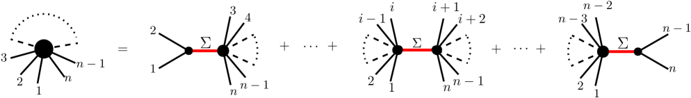
After showing that all $4$-point SSA can be expressed as the Lauricella functions, we consider the general $n$-point ($n\geq 5$) SSA now. The key is to apply the string theory extension of field theory BCFW on-shell recursion relations. We first consider the KN amplitude. Applying the BCFW deformation $\hat{k}_{1}\left(z\right)=k_{1}+zq$ and $\hat{k}_{n}\left(z\right)=k_{n}-zq$ with $q^{2}=k_{1}\cdot q=k_{n}\cdot q=0$, the locations of the poles $z_{m,M}$ are given by solutions of $\left(\hat{k}_{1}+k_{2}+....+k_{m}\right)^{2}+2(M-1)=0,$ $M=0,1,2...$. The $n$-point Koba-Nielsen (KN) amplitude can then be written as stringbcfw

$$A_{n}^{KN}=\underset{m=2}{\overset{n-2}{\sum}}\underset{M=0}{\overset{\infty}{\sum}}\frac{2R_{m+1,n-m+1}^{M}}{\left(k_{1}+k_{2}+...+k_{m}\right)^{2}+2(M-1)},$$ (11)

which is represented in Fig.1.
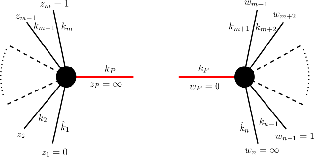
Refer to caption
Figure 1: Residues of KN amplitudes

It turns out that the residue $R_{m+1,n-m+1}^{M}$ in Eq.(11) can be calculated and expressed in terms of the subamplitudes LLY3

$$R_{m+1,n-m+1}^{M}=\sum_{P}A_{m+1}^{L}\left(1,\cdots,m,-P\right)A_{n-m+1}^{R}\left(P,m+1,\cdots n\right)$$ (12)

where

$\displaystyle A_{m+1}^{L}\left(1,\cdots,m,-P\right)$
$\displaystyle=\int_{0}^{1}dz_{m-1}\cdots\int_{0}^{z_{3}}dz_{2}\underset{1\leq j<i\leq m}{\prod}\left(z_{i}-z_{j}\right)^{k_{i}\cdot k_{j}}\prod_{r=1}\frac{\left[\underset{\sigma=1}{\overset{N_{r}}{{\displaystyle\prod}}}\epsilon_{r}^{(\sigma)}\cdot\underset{2\leq i\leq m}{\sum}k_{i}\left(z_{i}\right)^{r}\right]}{\sqrt{N_{r}!r^{N_{r}}}},$ (13)
$\displaystyle A_{n-m+1}^{R}\left(P,m+1,\cdots n\right)$
$\displaystyle=\int_{0}^{1}dw_{n-2}\cdots\int_{0}^{w_{m+2}}dw_{+1}\underset{P=m\leq j<i\leq n-1}{\prod}\left(w_{i}-w_{j}\right)^{k_{i}\cdot k_{j}}\prod_{r=1}\frac{\left[\underset{\sigma=1}{\overset{N_{r}}{{\displaystyle\prod}}}(-\epsilon_{r}^{(\sigma)})\cdot\underset{m+1\leq i\leq n-1}{\sum}k_{i}\left(\frac{1}{w_{i}}\right)^{r}\right]}{\sqrt{N_{r}!r^{N_{r}}}}$ (14)

with $k_{P}=\hat{k}_{1}+\underset{i=2}{\overset{m}{\sum}}k_{i}$. It is understood that $k_{1}$ in Eq.(13) should be replaced by $\hat{k}_{1}$. The results in Eq.(13), Eq.(14) are consistent with a direct calculation from KN amplitude LLY3 . The diagram representation of Eq.(12) is given in Fig.2.

Refer to caption
Figure 2: The left and right subamplitudes

In extending the field theory BCFW to the string theory BCFW above, one encountered difficulty of poles at infinity. To resolve the problem, the authors of bcfw4 used the pomeron vertex operators in the Regge regime constructed by BPST RR6 to show the vanishing of the string amplitudes at large complex momenta provided that the Regge behavior of the deformed amplitude is power law falloff $\mathcal{M}(z)\sim z^{n+1+\frac{t}{2}}$ (for sufficiently negative $t$) where $n$ depends on the mass levels. Indeed, the universal power law falloff behavior $V\sim[ik_{2}\cdot\partial X]^{1+\frac{t}{2}}$ Tan for arbitrary massive pomeron vertex and their associated universal power law falloff Regge amplitudes $A_{Regge}$ โˆผs1+t2similar-toabsentsuperscript๐‘ 1๐‘ก2\sim s^{1+\frac{t}{2}} KLY had all been shown to be independent of the mass levels of the vertex ($n=0$).

V Expressing n-point SSA in terms of LSSA

In the last subsection, we have shown in Eq.(11) and Eq.(12)ย that the $n$-point KN amplitude can be expressed in terms of product of lower-point sub-amplitudes. The next step is to consider $n$-point SSA with tensor legs. To do it, we introduce the following shifting principle:

Shifting principle : If the $n$-point KN amplitude $A_{n}^{KN}$ can be expressed in terms of the LSSA, then one can use the shifting method to calculate all $n$-point SSA $A_{n}$ with tensor legs (excited string states) and express them in terms of the LSSA ($\left(z_{1},z_{n-1},z_{n}\right)=\left(0,1,\infty\right)$)

$$A_{n}(k_{i}\cdot k_{j};\zeta_{k})\sim{\displaystyle\sum}c(k_{i};\zeta_{k})A_{n}^{KN}(k_{i}\cdot k_{j}\rightarrow k_{i}\cdot k_{j}-a_{ij}).$$ (15)

In Eq.(15), $k_{i}\cdot k_{j}$ with $1\leq i<j\leq n-1$ (kiโ‹…kjโ‰ k1โ‹…knโˆ’1)โ‹…subscript๐‘˜๐‘–subscript๐‘˜๐‘—โ‹…subscript๐‘˜1subscript๐‘˜๐‘›1(k_{i}\cdot k_{j}\neq k_{1}\cdot k_{n-1}) are kinematic variables of the $n$-point SSA which sums up to $\frac{(n-1)(n-2)}{2}-1=$ $\frac{n(n-3)}{2}$, $a_{ij}$ are shifting integers and $\zeta_{k}$ are polarizations of the excited string states.

For example, for a $5$-point SSA with four tachyons and one vector ($\left(z_{1},z_{4},z_{5}\right)=\left(0,1,\infty\right)$) LLY3

$\displaystyle A_{5}\left(\zeta_{1},k_{1};k_{2};k_{3};k_{4};k_{5}\right)$
$\displaystyle=\int_{0}^{1}dz_{3}\int_{0}^{z_{3}}dz_{2}z_{2}^{k_{2}\cdot k_{1}}z_{3}^{k_{3}\cdot k_{1}}\left(1-z_{3}\right)^{k_{4}\cdot k_{3}}\left(1-z_{2}\right)^{k_{4}\cdot k_{2}}\left(z_{3}-z_{2}\right)^{k_{3}\cdot k_{2}}(-\zeta_{1})\cdot\left[\frac{k_{2}}{z_{2}}+\frac{k_{3}}{z_{3}}+\frac{k_{4}}{1}\right]$
$\displaystyle=A_{5}^{(1)}+A_{5}^{(2)}+A_{5}^{(3)}.$ (16)

where one reads (a12=1,aiโ€‹jโ‰ 12=0)formulae-sequencesubscript๐‘Ž121subscript๐‘Ž๐‘–๐‘—120\left(a_{12}=1,a_{ij\neq 12}=0\right) for $A_{5}^{(1)}$, (a13=1,aiโ€‹jโ‰ 13=0)formulae-sequencesubscript๐‘Ž131subscript๐‘Ž๐‘–๐‘—130\left(a_{13}=1,a_{ij\neq 13}=0\right) for $A_{5}^{(2)}$ and $a_{ij}=0$ for $A_{5}^{(3)}$. The result can be shown to be a sum of LSSA. Mathematically, the calculation of all three terms of Eq.(16) are similar to that of the $5$-point KN amplitude with shifting some appropriate kinematic variables. Although the calculation of $5$-point SSA with higher tensor legs is very lengthy, it is trivial by the shifting method adopted in the calculation of Eq.(16) to see that all of them are LSSA.

We see that while the string on-shell recursion relation can be used to reduce higher point KN amplitudes to the lower SSA and express them in terms of the LSSA, the shifting method can be used to express SSA with tensor legs in terms of the LSSA.

In general, we can use mathematical induction, together with the on-shell recursion and the shifting principle, to show that all $n$-point SSA can be expressed in terms of the LSSA. The procedure goes as following. We assume that all $k$-point SSA ($k\leq n-1$) are LSSA, and we want to prove that all $n$-point SSA are LSSA. To prove this, we first apply the on-shell recursion to express the residue of $n$-point KN amplitude calculated in Eq.(12) in terms of the lower point ($k\leq n-1$) SSA which were assumed to be LSSA. So the $n$-point KN amplitude is a LSSA. We can then apply the shifting principle to show that all $n$-point SSA including the $n$-point KN amplitude are LSSA. This completes the proof.
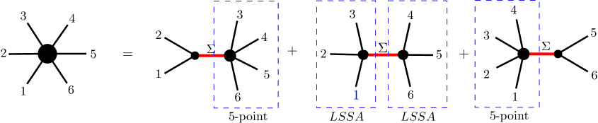
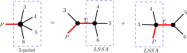
Finally, we use the example of $6$-point KN amplitude to demonstrate its LSSA form. See Fig.3 and Fig.4. We note that to show the $6$-point KN amplitude is a LSSA, one needs only do $1$-step recursion to express it in terms of the lower $5$-point and $4$-point amplitudes as was shown in Fig.3. Since we have shown that all $5$-point and $4$-point SSA are LSSA, the $6$-point KN amplitude is a LSSA. However, to explicitly calculate the LSSA form of the $6$-point KN amplitude, one needs to do the second recursion on the first and the third diagrams of Fig.3 as was shown in Fig.4, and the calculation will be very lengthy as there are two higher excited string states (two heavy lines) involved. In general, the residues of the $n$-point KN amplitude can be expressed as a LSSA with application of up to (rโ€‹eโ€‹cโ€‹uโ€‹rโ€‹sโ€‹iโ€‹oโ€‹n)nโˆ’4superscript๐‘Ÿ๐‘’๐‘๐‘ข๐‘Ÿ๐‘ ๐‘–๐‘œ๐‘›๐‘›4(recursion)^{n-4}.

Refer to caption
Figure 3: Expressing the 6-point KN amplitude in terms of the LSSA by the first recursion
Refer to caption
Figure 4: Expressing the 6-point KN amplitude in terms of the LSSA by the second recursion

$\boldsymbol{Applications.}$

VI Applications

After showing that all open bosonic SSA can be expressed in terms of the LSSA, we will demonstrate three applications of the associated $SL(K+3,C)$ Symmetry of LSSA on SSA:

VI.1 Solvability

The first one is to use $SL(K+3,C)$ group to solve all SSA and express them in terms of one amplitude. We first show that there exist $K+2$ recurrence relations for the $D$-type Lauricella functions. To do this, one begins with the type-$1$ Appell functions. For the case of $K=2$, the $D$-type Lauricella functions $F_{D}^{(K)}\left(\alpha;\beta_{1},...,\beta_{K};\gamma;x_{1},...,x_{K}\right)$ reduce to the type-$1$ Appell functions $F_{1}\left(\alpha;\beta_{1},\beta_{2};\gamma,x,y\right)$, and one has $4$ known recurrence relations. It was then shown that one can generalize the $4=2+2$ fundamental recurrence relations of the Appell functions $F_{1}$ and prove the following $K+2$ recurrence relations for the $D$-type Lauricella functions $(m=1,2,...,K)$ Group

$\displaystyle\left(\alpha-\underset{i}{\sum}\beta_{i}\right)F_{D}^{(K)}-\alpha F_{D}^{(K)}\left(\alpha+1\right)+\beta_{1}F_{D}^{(K)}\left(\beta_{1}+1\right)+...+\beta_{K}F_{D}^{(K)}\left(\beta_{K}+1\right)$ $\displaystyle=0,$ (17)
$\displaystyle\gamma F_{D}^{(K)}-\left(\gamma-\alpha\right)F_{D}^{(K)}\left(\gamma+1\right)-\alpha F_{D}^{(K)}\left(\alpha+1;\gamma+1\right)$ $\displaystyle=0,$ (18)
$\displaystyle\gamma F_{D}^{(K)}+\gamma(x_{m}-1)F_{D}^{(K)}\left(\beta_{m}+1\right)+(\alpha-\gamma)x_{m}F_{D}^{(K)}\left(\beta_{m}+1,;\gamma+1\right)$ $\displaystyle=0$ (19)

where for simplicity we have omitted those arguments of $F_{D}^{(K)}$ which remain the same in the relations. Moreover, these recurrence relations can be used to reproduce the Cartan subalgebra and simple root system of the $SL(K+3,C)$ group with rank $K+2$ Group . With the Cartan subalgebra and the simple roots, one can easily write down the whole Lie algebra of the $SL(K+3,C)$ group. So one can construct the $SL(K+3,C)$ Lie algebra from the recurrence relations and vice versa

Sโ€‹Lโ€‹(K+3,C)โ€‹ย Lie algebraย โŸบย Recurrence relations of Lauricella.โŸบ๐‘†๐ฟ๐พ3๐ถย Lie algebraย ย Recurrence relations of Lauricella.SL(K+3,C)\text{ Lie algebra }\Longleftrightarrow\text{ Recurrence relations of Lauricella.} (20)

The next step is to use the above recurrence relations to deduce the following key recurrence relation solve

$$x_{j}F_{D}^{(K)}\left(\beta_{i}-1\right)-x_{i}F_{D}^{(K)}\left(\beta_{j}-1\right)+\left(x_{i}-x_{j}\right)F_{D}^{(K)}=0,$$ (21)

which can be repeatedly used to decrease the value of $K$ and reduce all the Lauricella functions $F_{D}^{(K)}$ in the LSSA to the Gauss hypergeometric functions $F_{D}^{(1)}=$ ${}_{2}F_{1}(\alpha,\beta,\gamma,x)$. One can further reduce the Gauss hypergeometric functions by deriving a multiplication theorem for them, and then solve solve all the LSSA in terms of one single amplitude, say the four tachyon amplitude. See the recent review LSSA . For the cases of higher point functions in Eq.(10), all amplitudes can be solved and expressed in terms of sum of products of the four tachyon amplitudes. One of the reason of this solvability is that all $\beta_{J}$ in the Lauricella functions of the LSSA take very special values, namely, nonpositive integers.

VI.2 Iteration Relations

The second application is to use the $SL(K+3,C)$ symmetry to show the existence of iteration relations among residues of a given SSA so as to soften its hard scattering behavior. It is well known that one can express the Veneziano amplitude in terms of a series of simple pole terms with residues

A4=โˆ‘n=0โˆžโˆ’(ฮฑโ€‹(t)+1)โ€‹(ฮฑโ€‹(t)+2)โ€‹โ‹ฏโ€‹(ฮฑโ€‹(t)+n)n!โ€‹1ฮฑโ€‹(s)โˆ’nsubscript๐ด4infinity๐‘›0๐›ผ๐‘ก1๐›ผ๐‘ก2โ‹ฏ๐›ผ๐‘ก๐‘›๐‘›1๐›ผ๐‘ ๐‘›A_{4}=\overset{\infty}{\underset{n=0}{\sum}}-\frac{(\alpha(t)+1)(\alpha(t)+2)\cdots(\alpha(t)+n)}{n!}\frac{1}{\alpha(s)-n} (22)

where $\alpha(t)=\alpha^{\prime}t+\alpha(0)$ with $\alpha^{\prime}=1/2$ and $\alpha(0)=1$ GSW . Instead of naive $\sum\frac{1}{n}$ divergence, $A_{4}$ above behaves as exponential fall-off in the hard scattering limit due to the iteration relations of the residues among each pole term. We will find generalization of the iteration relations among residues in $A_{4}$ for higher point KN amplitudes in the following. We note that because of the solvability discussed in subsection $\boldsymbol{(A)}$ or the $SL(K+3,C)$ symmetry of the LSSA, we expect relations among various residues $M=0,1,2\ldots$of a given $R_{m+1,n-m+1}^{M}$ which is a sum of LSSA for a fixed $M$ and $(m,n)$. Indeed, if we define

$\displaystyle F_{M}\left(x_{1},\cdots,x_{n}\right)$ $\displaystyle\equiv\underset{\begin{array}[c]{c}a_{1}+\cdots+a_{n}=M\\ a_{1},\cdots,a_{n}=0\end{array}}{\sum}\frac{\left(T_{1}\right)_{a_{1}}}{a_{1}!}\cdots\frac{\left(T_{n}\right)_{a_{n}}}{a_{n}!}x_{1}^{a_{1}}\cdots x_{n}^{a_{n}}$ (25)
$\displaystyle=\underset{\left\{N_{r}\right\}\text{,with fixed }M=\underset{r}{\sum}rN_{r}}{\sum}\prod_{r=1}\left(\frac{1}{N_{r}!r^{N_{r}}}\left[T_{1}x_{1}^{r}+\cdots+T_{n}x_{n}^{r}\right]^{N_{r}}\right),$ (26)

one can prove the second equality in Eq.(26). We can now express the residue $R_{m+1,n-m+1}^{M}$ in terms of $F_{M}$

$\displaystyle R_{m+1,n-m+1}^{M}\left(\hat{1},2,\cdots,m,m+1,\cdots,n-1,\hat{n}\right)$
$\displaystyle=\int_{0}^{1}dz_{m-1}\cdots\int_{0}^{z_{3}}dz_{2}\int_{0}^{1}dw_{n-2}\cdots\int_{0}^{w_{m+2}}dw_{m+1}\underset{1\leq j<i\leq m}{\prod}\left(z_{i}-z_{j}\right)^{k_{i}\cdot k_{j}}$
$\displaystyle\times\underset{P=m\leq j<i\leq n-1}{\prod}\left(w_{i}-w_{j}\right)^{k_{i}\cdot k_{j}}F_{M}\left(\frac{z_{j}}{w_{i}}\right)$ (27)

where $j=2,\cdots,m;i=m+1,\cdots,n-1$ and $z_{m}=w_{n-1}=1$, and show the following iteration relation

$$F_{M}=\frac{1}{M}\underset{N=0}{\overset{M-1}{\sum}}F_{N}\left[\underset{2\leq j\leq m,m+1\leq i\leq n-1}{\sum}\left(-k_{j}\cdot k_{i}\right)\left(\frac{z_{j}}{w_{i}}\right)^{M-N}\right],$$ (28)

which expresses $F_{M}$ in terms of $F_{M-1}$, $F_{M-2}$, $....$, $F_{1}$, $F_{0}\equiv 1$. For illustration, we give one explicit example here. The $n=4$ term in the Veneziano amplitude $A_{4}$ can be written as

$$A_{4}=\cdots+\left(\underset{\alpha_{-4}}{\underbrace{\frac{T}{4}}}+\underset{\alpha_{-3}\alpha_{-1}}{\underbrace{\frac{T^{2}}{1!1!}\frac{1}{1^{1}}\frac{1}{3^{1}}}}+\underset{\alpha_{-2}^{2}}{\underbrace{\frac{T^{2}}{2!}\frac{1}{2^{2}}}}+\underset{\alpha_{-1}^{2}\alpha_{-2}}{\underbrace{\frac{T^{3}}{2!1!}\frac{1}{1^{2}2^{1}}}}+\underset{\alpha_{-1}^{4}}{\underbrace{\frac{T^{4}}{4!}\frac{1}{1^{4}}}}\right)\int_{0}^{1}dzz^{k_{1}\cdot k_{2}+4}+\cdots$$ (29)

where $T=-k_{2}\cdot k_{3}$. On the other hand, the explicit form of the residue $R_{4,3}^{4}$ of the $5$-point KN amplitude can be calculated to be

$\displaystyle R_{4,3}^{4}$ $\displaystyle=\frac{1}{4}\int_{0}^{1}dz_{2}z_{2}^{\hat{k}_{1}\cdot k_{2}}\left(1-z_{2}\right)^{k_{2}\cdot k_{3}}\left[-k_{3}\cdot k_{4}-(-k_{2}\cdot k_{4})z_{2}^{4}\right]$
$\displaystyle+\frac{1}{1!1!}\left(\frac{1}{3}\right)\left(\frac{1}{1}\right)\int_{0}^{1}dz_{2}z_{2}^{\hat{k}_{1}\cdot k_{2}}\left(1-z_{2}\right)^{k_{2}\cdot k_{3}}\left[-k_{3}\cdot k_{4}-(-k_{2}\cdot k_{4})z_{2}^{3}\right]\left[-k_{3}\cdot k_{4}-(-k_{2}\cdot k_{4})z_{2}\right]$
$\displaystyle+\frac{1}{2!}\left(\frac{1}{2}\right)^{2}\int_{0}^{1}dz_{2}z_{2}^{\hat{k}_{1}\cdot k_{2}}\left(1-z_{2}\right)^{k_{2}\cdot k_{3}}\left[-k_{3}\cdot k_{4}-(-k_{2}\cdot k_{4})z_{2}^{2}\right]^{2}$
$\displaystyle+\frac{1}{2!1!}\left(\frac{1}{1}\right)^{2}\left(\frac{1}{2}\right)\int_{0}^{1}dz_{2}z_{2}^{\hat{k}_{1}\cdot k_{2}}\left(1-z_{2}\right)^{k_{2}\cdot k_{3}}\left[-k_{3}\cdot k_{4}-(-k_{2}\cdot k_{4})z_{2}\right]^{2}\left[-k_{3}\cdot k_{4}-(-k_{2}\cdot k_{4})z_{2}^{2}\right]$
$\displaystyle+\frac{1}{4!}\left(\frac{1}{1}\right)^{4}\int_{0}^{1}dz_{2}z_{2}^{\hat{k}_{1}\cdot k_{2}}\left(1-z_{2}\right)^{k_{2}\cdot k_{3}}\left[-k_{3}\cdot k_{4}-(-k_{2}\cdot k_{4})z_{2}\right]^{4}.$ (30)

We see that the coefficients of each of the $5$ terms in Eq.(30) and Eq.(29) are the same! Furthermore, we have the correspondence $\alpha_{-l}\Longrightarrow\left[-k_{3}\cdot k_{4}-(-k_{2}\cdot k_{4})z_{2}^{l}\right]$. Similarly, $R_{4,3}^{0}$, $R_{4,3}^{1}$, $R_{4,3}^{2}$ and $R_{4,3}^{3}$ (and the corresponding $R_{3,4}^{M}$) can all be expressed in terms of the LSSA. Moreover, because of the solvability or the $SL(K+3,C)$ symmetry of the LSSA, we expect relations among various residues $R_{4,3}^{0}$, $R_{4,3}^{1}$, $R_{4,3}^{2}$, $R_{4,3}^{3}$, $R_{4,3}^{4}\cdots$ and $R_{3,4}^{0}$, $R_{3,4}^{1}$, $R_{3,4}^{2}$, $R_{3,4}^{3}$, $R_{3,4}^{4}\cdots$ of the $5$-point KN amplitude as was given in Eq.(28) and Eq.(27).

VI.3 Linear Relations

It was first observed that for each fixed mass level $N$ with $M^{2}=2(N-1)$, the following states are of leading order in energy at the hard scattering limit CHLTY2 ; CHLTY1

$$\left|N,2m,q\right\rangle\equiv(\alpha_{-1}^{T})^{N-2m-2q}(\alpha_{-1}^{L})^{2m}(\alpha_{-2}^{L})^{q}|0,k\rangle.$$ (31)

One important application of the LSSA presented in Eq.(2) is to reproduce LLY2 infinite linear relations among all hard $4$-point SSA and solve the ratios among them CHLTY2 ; CHLTY1

$$\frac{A^{(N,2m,q)}}{A^{(N,0,0)}}=\left(-\frac{1}{M}\right)^{2m+q}\left(\frac{1}{2}\right)^{m+q}(2m-1)!!.$$ (32)

These high energy behaviors of string theory GM ; GM1 were first conjectured by Gross Gross and later corrected and proved ChanLee ; ChanLee2 ; CHLTY2 ; CHLTY1 by the method of decoupling of zero norm states (ZNS) Lee ; lee-Ov ; LeePRL .

Since the linear relations obtained by the decoupling of ZNS are valid order by order and share the same forms for all orders in string perturbation theory, one expects that there exists stringy symmetry of the theory associated with the ratios in Eq.(32). In fact, there is a simple analogy from the ratios of the nucleon-nucleon scattering processes in particle physics $(a)$ ย p+pโ†’d+ฯ€+,(b)โ†’๐‘๐‘๐‘‘superscript๐œ‹๐‘p+p\rightarrow d+\pi^{+},(b) ย p+nโ†’d+ฯ€0โ†’๐‘๐‘›๐‘‘superscript๐œ‹0p+n\rightarrow d+\pi^{0} and $(c)$ ย n+nโ†’d+ฯ€โ†’๐‘›๐‘›๐‘‘๐œ‹n+n\rightarrow d+\pi, which can be calculated to be (ignore the mass difference between proton and neutron) $A_{a}:A_{b}:A_{c}=1:\frac{1}{\sqrt{2}}:1$ from $SU(2)$ isospin symmetry. Two such symmetry groups were suggested recently to be the $SL(5,C)$ group in the Regge string scattering limit review ; over and the $SL(4,C)$ group in the Non-relativistic string scattering limit review ; over . Moreover, it was shown that the ratios in Eq.(32) can be extracted from the Regge SSA review ; over . With the discovery of the LSSA, we now understand that the ratios in Eq.(32) are associated with the exact $SL(K+3,C)$ group LLY2 . Finally, For the cases of higher point $(n\geq 5)$ functions in Eq.(10), it is conjectured that there exist hard scattering regimes for which the linear relations persist and the ratios can be solved accordingly.

VII Conclusion

xWe conclude the discussion in this letter with the following analogy of fundamental symmetries between field theory and string theory

$\displaystyle SU(2)\text{ symmetry }$ โŸนย Yang-Millsย fieldย theory,โŸนabsentย Yang-Millsย fieldย theory,\displaystyle\Longrightarrow\text{ Yang-Mills {field} theory,} (33)
Bosonic open string theory โŸนย โ€‹Sโ€‹Lโ€‹(K+3,C)โ€‹ย symmetry,โŸนabsentย ๐‘†๐ฟ๐พ3๐ถย symmetry,\displaystyle\Longrightarrow\text{ }SL(K+3,C)\text{ symmetry,} (34)
$\displaystyle SU(2)\text{ slavnov-Taylor identities }$ $\displaystyle\Longleftrightarrow SL(K+3,C)\text{ recurrence relations.}$ (35)

This work is supported in part by the Ministry of Science and Technology (MoST) and S.T. Yau center of National Yang Ming Chiao Tung University (NYCU), Taiwan.

References

  • (1) C.N.Yang, โ€Hermann Weylโ€™s contribution to physicsโ€ in Hermann Weyl, ed. K. Chandlagrasekharan, Springer-Verlag 1980.
  • (2) Sheng-Hong Lai, Jen-Chi Lee, and Yiย Yang. The Lauricella functions and exact string scattering amplitudes. Journal of High Energy Physics, 2016(11):62, 2016.
  • (3) S. H. Lai, J. C. Lee and Yi Yang, โ€The $SL(K+3,C)$ Symmetry of the Bosonic String Scattering Amplitudesโ€, Nucl. Phys. B 941 (2019) 53-71.
  • (4) Willard Millerย Jr. Symmetry and separation of variables. Addison-Wesley, Reading, Massachusetts, 1977.
  • (5) S. H. Lai, J. C. Lee and Yi Yang, โ€Solving Lauricella String Scattering Amplitudes through recurrence relationsโ€, JHEP 09 (2017) 130.
  • (6) S. H. Lai, J. C. Lee and Yi Yang, โ€Recent developments of the Lauricella string scattering amplitudes and their exact $SL(K+3,C)$ Symmetryโ€, Symmetry 13 (2021) 454, arXiv:2012.14726 [hep-th].
  • (7) Davidย J Gross and Paulย F Mende. The high-energy behavior of string scattering amplitudes. Phys. Lett. B, 197(1):129โ€“134, 1987.
  • (8) Davidย J Gross and Paulย F Mende. String theory beyond the Planck scale. Nucl. Phys. B, 303(3):407โ€“454, 1988.
  • (9) Davidย J. Gross. High-Energy Symmetries of String Theory. Phys. Rev. Lett., 60:1229, 1988.
  • (10) Chuan-Tsung Chan and Jen-Chi Lee. Stringy symmetries and their high-energy limits. Phys. Lett. B, 611(1):193โ€“198, 2005.
  • (11) Chuan-Tsung Chan and Jen-Chi Lee. Zero-norm states and high-energy symmetries of string theory. Nucl. Phys. B, 690(1):3โ€“20, 2004.
  • (12) Chuan-Tsung Chan, Pei-Ming Ho, Jen-Chi Lee, Shunsuke Teraguchi, and Yiย Yang. High-energy zero-norm states and symmetries of string theory. Phys. Rev. Lett., 96(17):171601, 2006.
  • (13) Chuan-Tsung Chan, Pei-Ming Ho, Jen-Chi Lee, Shunsuke Teraguchi, and Yiย Yang. Solving all 4-point correlation functions for bosonic open string theory in the high-energy limit. Nucl. Phys. B, 725(1):352โ€“382, 2005.
  • (14) Jen-Chi Lee. New symmetries of higher spin states in string theory. Physics Letters B, 241(3):336โ€“342, 1990.
  • (15) Jen-Chi Lee and Burtย A Ovrut. Zero-norm states and enlarged gauge symmetries of the closed bosonic string with massive background fields. Nucl. Phys. B, 336(2):222โ€“244, 1990.
  • (16) Jen-Chi Lee. Decoupling of degenerate positive-norm states in string theory. Phys. Rev. Lett., 64(14):1636, 1990.
  • (17) Jen-Chi Lee and Yiย Yang. Review on high energy string scattering amplitudes and symmetries of string theory. arXiv preprint arXiv:1510.03297, 2015.
  • (18) Jen-Chi Lee and Yiย Yang. Overview of high energy string scattering amplitudes and symmetries of string theory. Symmetry, 11(8):1045, 2019.
  • (19) Gregory Moore. Symmetries of the bosonic string S-matrix. arXiv preprint hep-th/9310026, 1993.
  • (20) R. Boels, K.J. Larsen, N. A. Obers and Marcel Vonk, โ€œMHV, CSW and BCFW: field theory structures in string theory amplitudesโ€ย JHEP 0811 (2008) 015 [arXiv:0808.2598 [hep-th]].
  • (21) C. Cheung, D. Oโ€™Connell and B. Wecht, โ€œBCFW Recursion Relations and String Theory,โ€ย JHEP 1009 (2010) 052 [arXiv:1002.4674 [hep-th]].
  • (22) R. H. Boels, Daniele Marmiroli and N. A. Obers, โ€œOn-shell Recursion in String Theory,โ€ย JHEP 1010 (2010) 034 [arXiv:1002.5029 [hep-th]].
  • (23) Yung-Yeh Chang, Bo Feng, Chih-Hao Fu, Jen-Chi Lee,Yihong Wang and Yi Yang, โ€A note on on-shell recursion relation of string amplitudesโ€, JHEP 02 (2013) 028.
  • (24) R. Britto, F. Cachazo and B. Feng, โ€œNew recursion relations for tree amplitudes of gluons,โ€ย Nucl. Phys. B 715 (2005) 499 [hep-th/0412308].
  • (25) R. Britto, F. Cachazo, B. Feng and E. Witten, โ€œDirect proof of tree-level recursion relation in Yang-Mills theory,โ€ย Phys. Rev. Lett. 94 (2005) 181602 [hep-th/0501052].
  • (26) Sheng-Hong Lai, Jen-Chi Lee, Taejin Lee and Yiย Yang, Phys. Lett. B 776 (2018) 150-157.
  • (27) Taejin Lee, Phys. Lett. B 768 (2017) 248.
  • (28) Sheng-Hong Lai, Jen-Chi Lee, and Yiย Yang, โ€Residues of bosonic string scattering amplitudes and the Lauricella functionsโ€, arXiv:2109.08601 [hep-th].
  • (29) Richardย C Brower, Joseph Polchinski, Matthewย J Strassler, and Chung-I Tan. The Pomeron and gauge/string duality. JHEP, 2007(12):005, 2007.
  • (30) Chih-Hao Fu, Jen-Chi Lee, Chung-I Tan, and Yiย Yang. Recurrence relations of higher spin BPST vertex operators for open strings. Phys. Rev. D, 88(4):046004, 2013.
  • (31) Sheng-Lan Ko, Jen-Chi Lee, and Yiย Yang, โ€Patterns of high energy massive string scatterings in the Regge regimeโ€, JHEP 06 (2009) 028, arXiv:0812.4190 [hep-th].
  • (32) MB Green, JH Schwarz and E Witten. Superstring theory, v. 1. Cambridge University,Cambridge, (1987).