Accelerating Approximate Aggregation Queries with Expensive Predicates

Abstract.

Researchers and industry analysts are increasingly interested in computing aggregation queries over large, unstructured datasets with selective predicates that are computed using expensive deep neural networks (DNNs). As these DNNs are expensive and because many applications can tolerate approximate answers, analysts are interested in accelerating these queries via approximations. Unfortunately, standard approximate query processing techniques to accelerate such queries are not applicable because they assume the result of the predicates are available ahead of time. Furthermore, recent work using cheap approximations (i.e., proxies) do not support aggregation queries with predicates.

To accelerate aggregation queries with expensive predicates, we develop and analyze a query processing algorithm that leverages proxies (ABae). ABae must account for the key challenge that it may sample records that do not satisfy the predicate. To address this challenge, we first use the proxy to group records into strata so that records satisfying the predicate are ideally grouped into few strata. Given these strata, ABae uses pilot sampling and plugin estimates to sample according to the optimal allocation. We show that ABae converges at an optimal rate in a novel analysis of stratified sampling with draws that may not satisfy the predicate. We further show that ABae outperforms on baselines on six real-world datasets, reducing labeling costs by up to 2.3$\times$.

PVLDB Reference Format:
PVLDB, 14(11): 2341 - 2354, 2021.
doi:10.14778/3476249.3476285

1. Introduction

Analysts are interested in computing statistics over large, unstructured datasets where only a fraction of the data is of interest (i.e., with a selective predicate) with low computational cost. Machine learning (ML) methods are increasingly used to automatically answer such queries. For example, a media studies researcher may be interested in computing the average viewership (the statistic) of presidential candidates on TV news (the predicate) (Hong et al., 2020). To answer such queries, the researcher may deploy an expensive face detection deep neural network (DNN) to find all faces in the dataset and filter by presidential candidates, e.g.,

⬇

SELECT AVG(views) FROM video

WHERE contains_candidate(frame, ’Biden’)

Critically, these DNNs can be expensive to execute. For example, executing a state-of-the-art face detection DNN on the past year of MSNBC News would cost $262,000 on cloud compute infrastructure (NVIDIA V100, Amazon Web Services) (Zhang et al., 2018). Due to limited computational budgets, many organizations cannot exhaustively execute these expensive ML methods over the entirety of the dataset.

Fortunately, many applications can tolerate approximations (as is standard in the approximate query processing (AQP) literature (Li and Li, 2018)) so answering queries does not require exhaustively executing the expensive DNN. As is standard in AQP, a key requirement with approximate answers are statistical guarantees on query results. For example, the media studies researcher may require such guarantees to make precise claims about bias in TV news. Furthermore, these requirements are standard in scientific analyses. As such, we focus on queries with statistical guarantees in this work.

Unfortunately, standard techniques in AQP, ranging from histograms (Piatetsky-Shapiro and Connell, 1984), sketches (Braverman and Ostrovsky, 2013), and others (Agarwal et al., 2013), assume that the fields used in the predicates are already available, i.e., as structured records in a database. In contrast, we cannot precompute results as an expensive ML method is required to compute the predicate in our setting, e.g., we would have to execute an expensive face detector on every video frame to answer the query above. Recent work has focused on using cheap approximations (i.e., proxy models) to accelerate queries without having to pre-compute expensive DNNs (Kang et al., 2017; Kang et al., 2019; Kang et al., 2020a; Hsieh et al., 2018; Anderson et al., 2019). For example, a proxy for presidential candidates might be a cheap classifier in contrast to a full object detection DNN. Unfortunately, existing work either does not provide statistical guarantees on query accuracy (e.g., NoScope (Kang et al., 2017), Focus (Hsieh et al., 2018), Tahoma (Anderson et al., 2019)) or accelerates other query types (e.g., selection queries (Kang et al., 2020a), aggregation queries without predicates (Kang et al., 2019), and limit queries (Kang et al., 2019)).

We propose and analyze ABae (Aggregation with Expensive BinAry PrEdicates), a query processing algorithm leveraging stratified and pilot sampling (Kish, 1965) to accelerate linear aggregation queries (SUM, COUNT, and AVG) with expensive predicates and statistical guarantees on query accuracy. We further extend ABae to support common aggregation patterns, including queries with multiple predicates and with group by keys.

ABae leverages two key opportunities to accelerate such queries: proxy models and stratified sampling. That is, ABae splits the dataset into disjoint groups (strata), samples within strata, and computes a weighted average to obtain the final answer. ABae must account for three key challenges, as the predicate results are not available ahead of time: 1) strata selection, 2) budget allocation between strata, and 3) stochastic draws (i.e., sampling a record that may not match the predicate). We provide a principled stratification approach, leverage pilot sampling for budget allocation (Kish, 1965), and provide a novel analysis of stratified sampling with stochastic draws that shows that ABae converges at an optimal rate.

To address strata selection, ABae uses the proxy model. We assume the proxy provides information about the likelihood of a record satisfying the predicate (Kang et al., 2017, 2020a; Anderson et al., 2019; Hsieh et al., 2018). Since the proxy does not give information about the statistic, we stratify records by proxy score quantile. Under a mild monotonicity assumption on the proxy (Guo et al., 2017), this stratification will group records that are approximately equally likely to match the predicate in the same stratum. Intuitively, if the proxy is perfect (i.e., matches the predicate) and is independent of the statistic, this stratification will minimize the sampling variance. While ABae performs best when given proxy models which approximate the expensive predicate well, ABae still returns correct answers regardless of proxy model quality.

Given a stratification, our analysis shows that the optimal allocation depends on two key, per-strata quantities: the fraction of records that match the predicate ($p_{k}$) and the standard deviation of the statistic within a stratum ($\sigma_{k}$). Concretely, the optimal allocation is proportional to $\sqrt{p_{k}}\sigma_{k}$. However, we do not know these quantities ahead of time.

ABae proceeds in two stages to address this challenge. First, ABae will estimate $p_{k}$ and $\sigma_{k}$ using a fraction of the total sampling budget. Then, ABae will allocate the sampling budget using our plug-in estimates of $p_{k}$ and $\sigma_{k}$. We prove that ABae’s algorithm matches the expected error rates of the optimal stratified sampling allocation given the key quantities. Finally, to provide confidence intervals, ABae uses a bootstrapping procedure which only adds minimal computational overhead.

We also extend ABae to support group bys (ABae-GroupBy) and complex expressions involving multiple Boolean predicates (ABae-MultiPred). To support group by statements, we adapt our sample allocation strategy to minimize the maximum of the expected mean squared error of the groups (minimax error). We show a numerical optimization procedure can recover the optimal allocation for the minimax error. We also support combining multiple expensive predicates and their respective proxy models through negations, conjunctions, and disjunctions.

Finally, a key challenge in leveraging proxy models is to ensure efficient query answers despite potentially poor proxy model quality. Because ABae always produces valid results, we only need to address efficiency. To address this challenge, we derive a formula which computes the relative gain of using a given proxy. Then, by using a cheap procedure which can estimate the quantities in the formula, ABae can calculate expected performance gains of proxy models and select the best proxy model at query time.

We evaluate ABae and its extensions on six real-world datasets spanning text, images, and video. We show that ABae outperforms uniform sampling by up to 2.3$\times$. We also provide experiments to show that our methods for creating confidence intervals, executing group by aggregation queries, and forming complex predicates from multiple proxy models outperforms baselines.

In summary, our contributions are:

1. We develop ABae and its extensions, ABae-MultiPred and ABae-GroupBy, to accelerate aggregation queries with expensive predicates via proxy models.

2. We provide a theoretical analysis of ABae and show that it matches the expected error of the optimal stratified sampling algorithm asymptotically.

3. We evaluate these techniques on text, image, and video datasets, showing that ABae significantly outperforms uniform sampling.

2. Overview and Query Semantics

2.1. Overview

Target setting. ABae targets aggregation queries that contain one or more predicates that are expensive to evaluate. These predicates typically require executing expensive DNNs or querying human labelers. We assume the statistic can be computed in conjunction with the predicates or is cheap to compute. We support aggregation queries targeting AVG, SUM, and COUNT statistics. We do not support other aggregation types, such as COUNT DISTINCT or MAX.

Proxies. We further assume access to a proxy model per predicate, which returns a continuous value between $0$ and $1$. While not necessary for correctness, high quality proxies will return scores that are correlated with the predicate. These proxies can be orders of magnitude cheaper than oracles (e.g., over 4,000 images/second for the proxy vs 3 fps for the oracle (Kang et al., 2021b)). Thus, as is standard in the literature, we assume these proxies are substantially cheaper than the oracle methods so the proxies can be exhaustively executed over the entire dataset (Kang et al., 2017; Canel et al., 2019; Kang et al., 2019; Xu et al., 2019).

2.2. Examples

TV news. Consider a media studies researcher studying how the presence of presidential candidate affects viewership. The researcher is willing to query the expensive DNN at most 10,000 times and computes the average viewership with the following:

⬇

SELECT AVG(views) FROM news

WHERE contains_candidate(frame, ’Biden’)

ORACLE LIMIT 10,000 USING proxy(frame)

WITH PROBABILITY 0.95

where contains_candidate is computed via a face detection DNN and the proxy may be trained via specialization (Kang et al., 2017).

Traffic analysis. Consider an urban planner studying traffic patterns. The planner is interested in understanding waiting times at traffic lights and executes the following query

⬇

SELECT AVG(count_cars(frame)) FROM video

WHERE count_cars(frame) > 0

AND red_light(frame)

ORACLE LIMIT 1,000 USING proxy(frame)

WITH PROBABILITY 0.95

where count_cars is computed via an object detection DNN and red_light is computed by a human labeler. The proxy could be computed via an embedding index for unstructured data (Kang et al., 2020b).

Analyzing historical newspaper scans. Consider political scientists that are interested in computing statistics (e.g., fraction of articles with positive sentiment) over editorials (i.e., the predicate) in historical newspaper scans. Computing these statistics requires executing expensive OCR and text processing DNNs.

⬇

SELECT {AVG | SUM | COUNT} ({field | EXPR(field)})

FROM table_name WHERE filter_predicate

[GROUP BY key]

ORACLE LIMIT o USING proxy

WITH PROBABILITY p

Figure 1. Syntax for ABae. Users provide a statistic to compute, an expensive predicate, an oracle limit, proxy scores, and a success probability. As is standard for aggregation queries, users may specify a group by key.

2.3. Query Syntax and Semantics

We show the query syntax for ABae in Figure 1. As with standard AQP systems, ABae accepts a sampling budget and a probability of error and will return an approximate answer to the query and a confidence interval (CI). Our CI semantics are the standard frequentist CI semantics provided by other AQP systems (Agarwal et al., 2013). In particular, our CI semantics are valid regardless of proxy quality.

In contrast to standard AQP systems, ABae assumes that the predicate is expensive to evaluate. We refer to the methods to execute the predicates as “oracles” (Kang et al., 2020a; Kang et al., 2019). These oracles typically involve executing an expensive DNN and post-processing the result, e.g., executing Mask R-CNN to extract object types and positions from a frames of video and filtering by frames that contain at least two cars. Other use cases may require a human labeler. We further assume that the statistic is either cheap to compute or can be extracted by post-processing the oracle results.

To accelerate these queries, the user also provides a proxy function that computes per-record proxy scores for each predicate. These proxy scores are ideally correlated with the result of the predicate and substantially cheaper than the oracle predicates. Nonetheless, our algorithms will provide valid results even if the proxy scores are of poor quality: proxy correlation will only affect performance, not correctness.

ABae aims to return query results that minimize the mean squared error (MSE) between the approximate result and the result when exhaustively executing the query. ABae further aims to return CIs that are as tight as possible while maintaining the probability of success.

2.4. Query Formalism

Formally, let $\mathcal{D}=\{x_{i}\}$ be the set of data records, $O(x)\in\{0,1\}$ be the oracle predicate, and $X_{i}=f(x_{i})\in\mathbb{R}$ be the expression the query aggregates over. Let $\mathcal{D}^{+}=\{x\in\mathcal{D}:O(x)=1\}$. Finally, let $N$ be the sample budget.

ABae computes $\mu=\sum_{x\in\mathcal{D}^{+}}f(x)/|\mathcal{D}^{+}|$ via an approximation, $\hat{\mu}$, with a fixed sampling budget $N$. We measure query result quality by the MSE, i.e., $|\mu-\hat{\mu}|^{2}$. ABae returns a CI $[\underaccent{\bar}{\mu},\bar{\mu}]$. ABae further aims to minimize the length of the CI $\bar{\mu}-\underaccent{\bar}{\mu}$ subject to $\mu\in[\underaccent{\bar}{\mu},\bar{\mu}]$ with the specified probability and sample budget, over randomizations of the query procedure.

3. Algorithm Description and Query Processing

We describe ABae for accelerating aggregation queries with expensive predicates. We first describe accelerating queries with a single predicate. We then describe three natural extensions: queries with a group by key, queries with multiple predicates, and estimating proxy quality.

Table 1. Summary of notation.

Symbol	Description
$\mathcal{D}$	Universe of data records
$\mathcal{S}$	Stratification, i.e., $k$ strata
$\mathcal{P}(x)$	Proxy model
$N$	User-specified sampling budget
$K$	Number of strata
$\mathcal{O}(x)$	Oracle predicate
$X_{k,i}$	$i$th sample from stratum $k$
$p_{k}$	Predicate positive rate
${p_{\textrm{all}}}$	$\sum_{k}p_{k}$
$w_{k}$	Normalized $p_{k}$, i.e., $p_{k}/{p_{\textrm{all}}}$
$\mu_{k}$	$\mathbb{E}[X_{i,k}]$
$\mu_{\text{all}}$	$\sum p_{k}\mu_{k}/{p_{\textrm{all}}}$
$\sigma_{k}^{2}$	$Var[X_{i,k}]$
$N_{1}$	Number of samples in Stage 1
$N_{2}$	Number of samples in Stage 2

3.1. ABae with a Single Predicate

Overview. ABae leverages stratified sampling and pilot sampling (Kish, 1965) to accelerate aggregation queries with expensive predicates. Namely, ABae splits the dataset into disjoint subsets called strata. Then, ABae allocates sampling budget to the strata and combines the per-strata estimates to give the final estimate.

Our setting involves three distinct challenges. First, since not all records satisfy the predicate, we may not sample a valid record. This change, while seemingly simple, changes the optimal allocation and requires new theoretical analysis to prove convergence rates. Second, we must construct the strata without knowing which records satisfy the predicate. Third, we do not know $p_{k}$ (the predicate positive rate) and $\sigma_{k}$ (the standard deviation), which are necessary for computing the optimal allocation.

To address these issues, we leverage a two-stage sampling algorithm. ABae first estimates the key quantities necessary for optimal allocation: $p_{k}$ and $\sigma_{k}$ (also known as pilot sampling). ABae then uses these estimates to allocate sampling budget in the Stage 2. We show in Section 4 that ABae achieves an optimal rate.

Algorithm 1 Pseudocode for ABae. ABae proceeds in two stages. It first estimates $p_{k}$ and $\sigma_{k}$. It then samples according to the estimated optimal allocation, $\hat{T}_{k}=\sqrt{\hat{p}_{k}}\hat{\sigma}_{k}/\sum_{i=1}^{K}\sqrt{\hat{p}_{i}}\hat{\sigma}_{i}$.

1:function ABaeInit($\mathcal{D}$, $\mathcal{P}$, $K$)

2:     $\mathcal{D}\leftarrow Sort(\mathcal{D},\ key=lambda\ x:\mathcal{P}(x))$

3:     $\mathcal{S}_{1},...,\mathcal{S}_{K}\leftarrow\text{StratifyByQuantile}(\mathcal{D},K)$

4:     return $\mathcal{S}$

5:

6:function ABaeSample($\mathcal{S}$, $\mathcal{O}$, $K$, $N_{1}$, $N_{2}$, SampleFn)

7:     for each k in [1, …, K] do $\triangleright$ Stage 1

8:         $R_{k}^{(1)}\leftarrow\text{SampleFn}(\mathcal{S}_{k},N_{1})$ $\triangleright$ $R_{k}$ are sampled records

9:         $X_{k}^{(1)}\leftarrow\{f(x)\ |\ x\in R_{k}^{(1)},\ \mathcal{O}(x)=1\}$

10:         $\hat{\mu}_{k}$ $\leftarrow$ $\sum_{i=1}^{|X_{k}^{(1)}|}X_{k,i}^{(1)}/|X_{k}^{(1)}|$ if $|X_{k}^{(1)}|>0$ else $0$

11:         $\hat{p}_{k}$ $\leftarrow$ $|X_{k}^{(1)}|/|R_{k}^{(1)}|$

12:         $\hat{\sigma}^{2}_{k}$ $\leftarrow$ $\sum_{i=1}^{|X_{k}^{(1)}|}\frac{(X_{k,i}^{(1)}-\hat{\mu}_{k})^{2}}{|X_{k}^{(1)}|-1}$ if $|X_{k}^{(1)}|>1$ else $0$      

13:     for each k in [1, …, K] do

14:         $\hat{T}_{k}$ $\leftarrow$ $\sqrt{\hat{p}_{k}}\hat{\sigma}_{k}/\sum_{i=1}^{K}\sqrt{\hat{p}_{i}}\hat{\sigma}_{i}$      

15:     for each k in [1, …, K] do $\triangleright$ Stage 2

16:         $R_{k}^{(2)}\leftarrow R_{k}^{(1)}+\text{SampleFn}(\mathcal{S}_{k},\lfloor N_{2}\hat{T}_{k}\rfloor)$

17:         $X_{k}^{(2)}\leftarrow X_{k}^{(1)}+\{f(x)\ |\ x\not\in R_{k}^{(1)},\ x\in R_{k}^{(2)},\ \mathcal{O}(x)=1\}$

18:         $\hat{p}_{k}$ $\leftarrow$ $|X_{k}^{(2)}|/|R_{k}^{(2)}|$

19:         $\hat{\mu}_{k}$ $\leftarrow$ $\sum_{i=1}^{|X_{k}^{(2)}|}X_{k,i}^{(2)}/|X_{k}^{(2)}|$ if $|X_{k}^{(2)}|>0$ else $0$      

20:     return $\sum_{k=1}^{K}\hat{p}_{k}\hat{\mu}_{k}/\sum_{k=1}^{K}\hat{p}_{k}$, $R^{(2)}$

21:

22:function ABae($\mathcal{D}$, $\mathcal{O}$, $\mathcal{P}$, $K$, $N_{1}$, $N_{2}$)

23:     $\mathcal{S}\leftarrow\textsc{ABaeInit}(\mathcal{D},\mathcal{P},K)$

24:     $\text{SampleFn}\leftarrow\text{SampleWithoutReplacement}$

25:     $\hat{\mu},\ R^{(2)}\leftarrow\textsc{ABaeSample}(\mathcal{S},\mathcal{O},K,N_{1},N_{2},\text{SampleFn})$

26:     return $\hat{\mu}$

Formal description. Recall that $p_{k}$ is the predicate positive rate and that $\sigma_{k}^{2}$ is the variance of the statistic. Furthermore, recall that $\mathcal{D}$ is the full dataset, $O(x)$ is the oracle predicate, and $X_{i}$ are the samples. Denote $X_{k,i}$ to be the $i$th positive sample from stratum $k$.

Additionally, denote $K$ to be the number of strata, $N_{1}$ to be the number of samples in Stage 1, and $N_{2}$ to be the number of samples in Stage 2, which are parameters to ABae. ABae will compute several other quantities, including ${p_{\textrm{all}}}=\sum_{k}p_{k}$, $w_{k}=p_{k}/{p_{\textrm{all}}}$ the normalized $p_{k}$, and $\mu_{k}=\mathbb{E}[X_{k,i}]$ the per stratum mean. We summarize the notation in Table 1.

We present the pseudocode for the sampling algorithm in Algorithm 1. ABae creates the strata by ordering the records by proxy score and splitting into $K$ strata by quantile.

ABae will then perform a two-stage sampling procedure. In Stage 1, ABae samples $N_{1}$ samples from each of the $K$ strata to estimate $p_{k}$ and $\sigma_{k}$, which are the key quantities for determining optimal allocation. In Stage 2, ABae will allocate the remaining samples proportional to our estimates of the optimal allocation.

ABae construct plugin estimates for $p_{k}$ and $\mu_{k}$, denoted $\hat{p}_{k}$ and $\hat{\mu}_{k}$ respectively. To compute its final estimates, ABae will use all the samples from Stage 1 and Stage 2 to compute $\hat{p}_{k}$ and $\hat{\mu}_{k}$. ABae will return the estimate $\sum_{k}\hat{p}_{k}\hat{\mu}_{k}/\sum_{k}\hat{p}_{k}$ as the approximate answer.

As the final estimates are sensitive to the estimate of $p_{k}$, i.e., $\hat{p}_{k}$, we find that reusing samples between stages dramatically improves performance (Section 5.3).

We defer the proofs of convergence and rates to Section 4.

Confidence intervals. We use the non-parametric bootstrap (Efron and Tibshirani, 1994) to compute confidence intervals, which resamples existing samples. Since the per-stratum samples from both stages of ABae are independent and identically distributed (i.i.d.), we resample from samples across both stages.

Algorithm 2 Bootstrap procedure for computing CIs. We resample existing samples over both stages of the algorithm.

1:function Bootstrap($R^{(2)}$, $\mathcal{O}$, $K$, $N_{1}$, $N_{2}$, $\beta$, $\alpha$)

2:     for each b in [1, …, $\beta$] do $\triangleright$ $\beta$ is # of bootstrap trials

3:         for each k in [1, …, $K$] do

4:              $R_{k}^{*}\leftarrow\text{SampleWithReplacement}(R_{k}^{(2)},|R_{k}^{(2)}|)$

5:              $X_{k}^{*}\leftarrow\{f(x)\ |\ x\in R_{k}^{*},\ \mathcal{O}(x)=1\}$

6:              $\hat{p}_{k}^{*}\leftarrow|X_{k}^{*}|/|R_{k}^{*}|$

7:              $\hat{\mu}_{k}^{*}\leftarrow\sum_{i=1}^{|X_{k}^{*}|}X_{k,i}^{*}/|X_{k}^{*}|$ if $|X_{k}^{*}|>0$ else $0$          

8:         $\hat{\mu}_{b}\leftarrow\sum_{k=1}^{K}\hat{p}_{k}^{*}\hat{\mu}_{k}^{*}/\sum_{k=1}^{K}\hat{p}_{k}^{*}$      

9:     return $\text{Percentile}(\alpha/2,\ \hat{\mu}),\text{Percentile}(1-\alpha/2,\ \hat{\mu})$

10:

11:function ABaeWithCI($\mathcal{D}$, $\mathcal{O}$, $\mathcal{P}$, $K$, $N_{1}$, $N_{2}$, $\beta$, $\alpha$)

12:     $\mathcal{S}\leftarrow\textsc{ABaeInit}(\mathcal{D},\mathcal{P},K)$

13:     $\text{SampleFn}\leftarrow\text{SampleWithoutReplacement}$

14:     $\hat{\mu},\ R^{(2)}\leftarrow\textsc{ABaeSample}(\mathcal{S},\mathcal{O},K,N_{1},N_{2},\text{SampleFn})$

15:     return $\hat{\mu},\ \textsc{Bootstrap}(R^{(2)},\mathcal{O},K,N_{1},N_{2},\beta,\alpha)$

We present the pseudocode for the bootstrap procedure in Algorithm 2. ABae bootstraps across both stages of the sampling algorithm to form CIs. We formally show the validity of the bootstrap in an extended technical report (Kang et al., 2021a). We further show that our procedure produces CIs that are nominally correct in Section 5.

In standard AQP, the bootstrap is considered an expensive procedure as it requires resampling and recomputing the statistic. However, in our setting, we assume that the oracle predicate is expensive to execute. As a result, the bootstrap is computationally cheap compared to the cost of obtaining the samples. Concretely, in several of our experiments, executing 1,000 bootstrap trials using unoptimized Python code on a single CPU core is as expensive as executing 2,500 oracle calls on an NVIDIA T4 accelerator, which corresponds to under 0.3% of a medium-sized dataset.

Setting parameters. ABae requires setting two parameters: the fraction of samples between Stage 1 and 2 and the number of strata. We recommend using 30-50% of samples in Stage 1 and $K$ to be maximal such that every strata receives at least 100 samples in Stage 1. Our experiments show that ABae is not sensitive to these parameters, but that these settings tend to do best (Section 5.3).

3.2. Group Bys

We extend ABae to support queries with group by keys (ABae-GroupBy). We focus on minimizing the maximum error (minimax error) over groups. Other objectives can be supported (e.g., the sum of errors), but we defer optimizing other objectives to future work. As an example of a query with a group by key, consider:

⬇

SELECT COUNT(frame), person FROM VIDEO

WHERE person IN (’Biden’, ’Trump’)

GROUP BY person

where, for simplicity, we assume that person is a virtual field extracted by an expensive face detection DNN.

We assume that the group by key is expensive to compute and consider two different scenarios. In the first scenario, a single oracle determines the group key directly. For example, in the query above, a single oracle would directly classify a person as Biden or Trump. In the second scenario, there is an oracle per group, where each oracle can classify whether a record belongs to a specific group key or not. For example, in the query above, we must execute two oracles: one to classify whether or not a person is Biden and another for Trump. We have found this scenario to be common when practitioners do not build their own models. We separate these two cases as they have different optimization objectives.

To optimize the minimax error, we formulate the allocation of the samples to minimize the minimax error as a non-linear optimization problem. Concretely, consider the multiple oracle setting. Given a stratification of group $g$ (with a total of $G$ groups), denote the error of this stratification as $\textrm{Err}(g)/N$, for $N$ samples. Namely, $\textrm{Err}(g)/N$ is equivalent to the error when using a single predicate. Then, we aim to optimize the following objective

(1) $$\mathcal{L}=\min_{\Lambda\in[0,1]^{G},\sum_{l=1}^{G}\Lambda_{l}=1}\left(\max_{g}\frac{\textrm{Err}(g)}{\Lambda_{l}N}\right)$$

where $\Lambda$ is a weight vector corresponding to the sample allocation between groups. We show that this optimization problem can be numerically optimized using the Nelder-Mead simplex algorithm (Sorensen, 1982).

Concretely, ABae-GroupBy proceeds as follows:

1. Sample uniformly at random to estimate the quantities needed to compute $\textrm{Err}(g)$.

2. Solve Eq. 1 via the Nelder-Mead simplex algorithm (Sorensen, 1982).

3. Sample according to the allocation in the previous step.

4. Return the combined estimates.

We defer the full formulation to Section 4.5.

3.3. Complex Predicates

In addition to a queries with a single predicate, we extend ABae to support queries that contain any number of conjunctions, disjunctions, and negations (ABae-MultiPred). Presently, we assume that ABae-MultiPred receives as input a set of per-record proxy scores per predicate. We show an example of such a query in Section 2.2.

To answer such queries, ABae-MultiPred will combine the proxy scores from the predicates to obtain a single, per-record set of scores that ideally indicates the likelihood of a record matching the whole expression. ABae-MultiPred combines the proxy scores by transforming the expression into an arithmetic expression with the following substitutions:

1. Negations are replaced by subtraction from one.

2. Conjunctions are replaced by products.

3. Disjunctions are replaced by max.

ABae-MultiPred’s approach will return exact results if the proxies are perfectly calibrated and perfectly sharp. While this assumption does not hold in practice, we show that our approach works well in practice in Section 5.

3.4. Selecting Proxies

In some applications, users may have to select between several viable proxies for an expensive predicate. For example, suppose the user wishes to filter emails by spam. The user can provide several rule-based proxies in the form of detecting keywords, such as “money” or “$”.

A key question is which proxy will provide the lowest MSE for a given budget. To estimate performance improvements, ABae will use the samples from Stage 1. For each proxy, ABae will construct the strata and estimate the corresponding $p_{k}$ and $\sigma_{k}$. ABae will use the MSE formula for the perfect information, deterministic draws setting to estimate the optimal achievable MSE (Proposition 2). Given these estimates, ABae will take the top proxy as the proxy to use in the query. We note that this procedure can reuse samples and only adds negligible computational overhead.

Although the formula for the perfect information, deterministic draws setting does not directly apply, we find it is a good predictor of relative performance.

Finally, ABae can combine proxies by sampling randomly in Stage 1 and using these samples to train a logistic regression model using the proxies as features and the predicate as the target.

4. Theoretical Analysis

We present a statistical analysis of ABae and its extensions. We first show that a related sampling procedure achieves rate $O\left(\frac{1}{N}\right)$ assuming perfect knowledge of $p_{k}$ and $\sigma_{k}$. We then show that our sampling procedure matches the rate of the optimal strategy. Finally, we show that our optimization procedure for allocation for group by keys is optimal for the deterministic setting.

We provide the intuition and theorem statements in this manuscript. We defer the full proofs to an extended technical report (Kang et al., 2021a).

4.1. Notation and Preliminaries

Notation. Recall the notation in Table 1. We emphasize that $X_{k,i}$ is the $i$th positive sample from stratum $k$, i.e., the $i$th sample that satisfies the predicate. Furthermore, recall that $\mu_{k}$ is the per-stratum mean, ${p_{\textrm{all}}}=\sum p_{k}$ be the sum of the $p_{k}$, and $\mu_{\text{all}}$ be the overall mean. Finally, recall that $w_{k}=p_{k}/{p_{\textrm{all}}}$, the normalized predicate positive rate, which corresponds to the weighting of $\mu_{k}$ to $\mu_{\text{all}}$.

Assumptions and properties. We assume $X_{k,i}$ is sub-Gaussian with nonzero standard deviation, a standard assumption for stratified sampling (Carpentier et al., 2015). Sums of sub-Gaussian variables converge with quantitative rates and this assumption widely holds in practice. In particular, centered, bounded random variables are sub-Gaussian. The sub-Gaussian assumption gives the existence of universal constants such that $\mathbb{E}[|X_{k,i}|]\leq C^{(\mu)}$ and $Var[X_{i,k}]\leq C^{(\sigma^{2})}$.

We further assume that ${p_{\textrm{all}}}\geq C^{p_{\textrm{all}}}>0$, which enforces that at least one stratum has non-vanishing $p_{k}$.

4.2. Optimal Allocation with Deterministic Draws

We first analyze the setting where we assume perfect knowledge of $p_{k}$ and $\sigma_{k}$ and that we receive a deterministic, per-stratum number of draws given a sampling budget. Specifically, given a budget of $T_{k}N$ per stratum, we assume that we receive $p_{k}T_{k}N$ samples, rounded up. We prove the optimal allocation under a continuous relaxation and the rate when using this optimal allocation.

Proposition 1.

Suppose $p_{k}$ and $\sigma_{k}$ are known and we receive $B_{k}=p_{k}T_{k}N$ samples per stratum (up to rounding effects). Then, the choice $T_{k}=T_{k}^{*}$ that minimizes the MSE for the unbiased estimator $\hat{\mu}_{\text{all}}=\sum_{k}p_{k}\hat{\mu}_{k}/\sum_{k}p_{k}$ is

(2) $$T_{k}^{*}=\frac{\sqrt{p_{k}}\sigma_{k}}{\sum_{i=1}^{K}\sqrt{p_{i}}\sigma_{i}}$$

Proposition 2.

Suppose the conditions in Proposition 1 hold. Then, the squared error under the allocation $T_{k}^{*}$ is

(3) $$\mathbb{E}[(\hat{\mu}_{\text{all}}-\mu_{\text{all}})^{2}|B_{k}=p_{k}T_{k}^{*}N] =\sum_{k=1}^{K}\frac{w_{k}^{2}\sigma_{k}^{2}}{p_{k}T_{k}^{*}N}$$

(4) $$=\frac{1}{N{p_{\textrm{all}}}^{2}}\cdot\left(\sum_{k=1}^{K}\sqrt{p_{k}}\sigma_{k}\right)^{2}$$

Intuitively, these propositions say for deterministic draws, the optimal allocation downweights the standard importance sampling allocation by a factor of $\sqrt{p_{k}}$. The resulting MSE decreases linearly with respect to the sample budget and a scaling factor.

We note that uniform sampling with deterministic draws converges at rate $\frac{\sigma^{2}}{Np_{\textrm{avg}}}$, where $p_{\textrm{avg}}=\sum p_{k}/K$. As a result, stratified sampling offers room for improvement. For example, suppose $p_{1}=1$, $p_{k}=0$ for $k\neq 1$, and that $\sigma_{k}=1$ for all $k$. This corresponds to a perfect proxy and conditionally independent draws and statistic. Then, uniform sampling converges at rate $\frac{K}{N}$, in contrast to stratified sampling’s rate of $\frac{1}{N}$. This corresponds to a $K$-fold improvement in rate.

4.3. ABae with a Single Predicate

We analyze ABae’s two stage sampling algorithm, in which we do not know $p_{k}$ and $\sigma_{k}$. We provide the theorem statement, but defer the full proof to an extended technical report (Kang et al., 2021a). We assume that $N_{2}$ is suitably large relative to $N_{1}$ for the remainder of the paper.

Theorem 4.1.

With high probability over the draws made in Stage 1 and in expectation in Stage 2,

(5) $$\mathbb{E}[(\hat{\mu}_{\text{all}}-\mu_{\text{all}})^{2}]\leq O\left(\frac{1}{N_{1}}+\frac{1}{N_{2}}+\frac{\sqrt{N_{1}}}{\sqrt{N_{2}}}\cdot\frac{1}{N_{2}}\right)$$

Furthermore, if $N_{1}=N_{2}$

(6) $$\mathbb{E}[(\hat{\mu}_{\text{all}}-\mu_{\text{all}})^{2}]\leq O\left(\frac{1}{N}\right)$$

4.4. Understanding ABae

We provide an overall proof sketch of the analysis of ABae and highlight several aspects of the analysis of broader interest.

4.4.1. Proof Sketch

Our proof strategy proceeds as follows. We first show that our estimates $\hat{p}_{k}$ and $\hat{\sigma}_{k}$ converge to $p_{k}$ and $\sigma_{k}$ in a quantitative way (i.e., with a specific rate). As a result, our estimate for the optimal allocation will also converge in a quantitative way.

Given the estimate for the optimal allocation, we show that the number of draws in Stage 2 for all strata will approach the deterministic number of draws, for $p_{k}$ large enough (larger than $\frac{1}{N_{2}}$). We then show that the error converges appropriately for the strata with $p_{k}$ large enough and that the error for the remaining strata becomes negligible. As a result, our final estimate converges with rate $O(\frac{1}{N})$.

4.4.2. Challenges

We describe several challenges in the analysis of ABae. Prior work has focused on known, deterministic per-strata costs and variances. In contrast, our problem does not have a cost, but rather a stochastic probability of receiving useful information. We study this stochastic draw case and prove that using pilot sampling with plug-in estimates (Kish, 1965) is valid and near optimal.

Unknown $p_{k}$ and $\sigma_{k}$. Most work in stratified sampling assumes that features of the data distributions within each stratum are known and constructs optimal allocations of samples using this information. In our setting, these quantities must be estimated, which may not be possible when $p_{k}$ is small. For example, if $p_{k}=\frac{1}{N^{2}}$ for some stratum, then we may not draw even a single positive record from that stratum, making $p_{k}$ and $\sigma_{k}$ impossible to estimate.

Stochastic draws. In contrast to standard stratified sampling, we may draw a record that does not satisfy the predicate. As a result, for a fixed number of draws, the number of records matching a predicate is stochastic. Most work on stratified sampling assumes a deterministic allocation of samples to strata.

When the number of draws for some arbitrary $M$ from a stratum and the probability $p_{k}$ of matching the predicate are both large, the number of positive records concentrates around $p_{k}M$ and the resulting estimator has similar properties to one with $p_{k}M$ deterministic draws. However, if $p_{k}M$ is small, this analysis breaks down.

Fractional allocations. To show that ABae converges at the optimal rate, we compare to the setting of deterministic draws and perfect information. Given perfect information of $p_{k}$ and $\sigma_{k}$, the optimal allocation is given by Proposition 1 and its MSE is given by Proposition 2. However, this allocation cannot be achieved in general, as it results in fractional sampling. Nonetheless, we show that our sampling procedure, which rounds down the ideal fractional allocations, achieves the same $O\left(\frac{1}{N}\right)$ rate. Thus, rounding does not affect the convergence rate of our procedure.

4.4.3. Statistical Intuition

Our primary tool for dealing with unknown quantities and stochastic draws is dividing the strata into groups: where $p_{k}$ is large and where $p_{k}$ is small. Since the number of positive draws is Binomial, we apply standard convergence to the total number of positive draws when $p_{k}$ is large. For stratum where $p_{k}$ is small, the contribution of that stratum to the total error is at most $p_{k}C^{(\mu)}$, which does not increase the asymptotic error. To illustrate our technique, consider the following proposition.

Proposition 3.

Recall that $N_{1}$ and $N_{2}$ are the number of samples in Stages 1 and 2 respectively. With high probability in Stage 1 and if $N_{1}$ is a constant multiple of $N_{2}$ as $N$ grows, the MSE of the error in Stage 2 can be written as

(7) $$\mathbb{E} \left[(\hat{\mu}_{\text{all}}-\mu_{\text{all}})^{2}\right]=\sum_{k=1}^{K}\hat{w}_{k}^{2}\text{Var}(\hat{\mu}_{k})+O\left(\frac{1}{N_{1}}+\frac{1}{N_{2}}\right)$$

where $\hat{w}_{k}=\hat{p}_{k}/\sum\hat{p}_{k}$.

As shown in Eq. 7, the overall MSE is bounded above by the sum of $\hat{w}_{k}^{2}\text{Var}(\hat{\mu}_{k})$, which are per-strata quantities. We then bound these quantities for strata where $p_{k}$ is (quantitatively) large or small. Specifically, define $p_{*}=\frac{2\ln(1/\delta)+2\sqrt{\ln(1/\delta)}+2}{N_{1}}=O\left(\frac{1}{N_{1}}\right)$ for failure probability $\delta$. Furthermore, we assume that $N_{1}$ is a constant multiple of $N_{2}$ as $N$ grows. We divide the strata into cases based on whether $p_{k}>p_{*}$ or $p_{k}\leq p_{*}$

Consider the case where $p_{k}>p_{*}$. By standard concentration arguments, the number of positive samples in Stage 2 concentrates to its expectation, which is large. Thus, $\hat{w}_{k}^{2}\text{Var}(\hat{\mu}_{k})$ decays at rate (approximately) $O\left(\frac{1}{N_{2}}\right)$ by standard concentration arguments. For $p_{k}\leq p_{*}$, we can directly bound the contribution. To understand this, consider the following proposition.

Proposition 4.

(8) $$\hat{w}_{k}^{2}\text{Var}[\hat{\mu}_{k}] \leq\hat{w}_{k}^{2}\left(\mathbb{E}\left[\frac{\sigma_{k}^{2}}{B_{k}^{(2)}}|B_{k}^{(2)}>0\right]+P(B_{k}^{(2)}=0)\mu_{k}^{2}\right)$$

(9) $$\leq O\left(\frac{1}{N_{1}}+\frac{1}{N_{2}}+\frac{\sqrt{N_{1}}}{\sqrt{N_{2}}}\cdot\frac{1}{N_{2}}\right)$$

where $B_{k}^{(2)}$ is the number of positive draws in Stage 2.

Proof sketch.

The key challenge is bounding quantities involving $B_{k}^{(2)}$. Suppose counterfactually that $B_{k}^{(2)}$ were deterministic: then the expression would correspond to the standard variance of an i.i.d. estimator. Namely, the variance if an i.i.d. estimator decays as $1/B_{k}^{(2)}$. However, since we obtain a stochastic number of draws, we must condition on the event of non-zero draws and take the expectation. Since the draws are binomial in distribution, the leading order converges a.s. to its mean value, which would give the desired bound in this toy setting.

We now adapt this strategy to account for $B_{k}^{(2)}$ being stochastic in ABae. For $p_{k}>p_{*}$, $B_{k}^{(2)}$ is approximately $p_{k}T_{k}^{*}N_{2}$ with high probability. As a result, with high probability, each stratum had sufficient samples to form estimates. We can complete the proof similarly to the toy setting with deterministic $B_{k}^{(2)}$.

However, if $p_{k}<p_{*}$, we may not draw the requisite number of samples. For example, if $p_{k}=\frac{1}{N^{2}}$, we would not obtain any samples on average. Thus, our analysis must consider the case where $p_{k}<p_{*}$ separately. When $p_{k}$ is small, we can directly bound the contribution of the sum. Namely, $\hat{w}_{k}^{2}=O(1/N^{2})$ as $p_{k}\leq\frac{C_{1}}{N}$ and the remainder of the quantities are bounded by a constant.

Thus, the overall bound follows from considering the strata where $p_{k}$ is small and where $p_{k}$ is large. ∎

4.4.4. Overview of Techniques

We briefly describe two techniques used to prove the necessary bounds. First, we leverage exponential tail bounds on sums of Bernoulli random variables (Lemma 1 (Chung and Lu, 2002)). Both the upper and lower tail bounds are requires to show that $\sqrt{\hat{p}_{k}}$ converges to $\sqrt{p_{k}}$: this requires stronger tail bounds than showing $\hat{p}_{k}$ converges to $p_{k}$. Second, we use quantitative, exponential tail bounds on Binomial random variables (Tarjan, 2009) to bound the number of positive draws.

4.5. Analyzing Group Bys

Recall that we aim to optimize the minimax error for queries with a group by clause. Suppose there are $G$ groups and that we have a proxy per group. As in the case with a single predicate, each proxy induces a stratification over the dataset. Given these $G$ stratifications, ABae-GroupBy estimates the quantities necessary for optimal allocation and executes Stage 2 of ABae on each stratification appropriately. Thus, the key question is how to allocate samples between the stratifications. We first demonstrate how to allocate samples in the perfect information, deterministic setting and use our plug-in estimates for allocation estimation.

For this section, we index the stratification by $l$, the group by $g$, and the strata by $k$. Thus, $p_{l,g,k}$, $\sigma_{l,g,k}$, and $\mu_{l,g,k}$ denote the predicate positive rate, the standard deviation, and the stratum mean in stratification $l$, group $g$, and strata $k$ respectively.

To accelerate group by queries, we rely on ABae as a subroutine. When we say that we execute an instance of ABae with a stratification $l$, we mean that we stratify the dataset using the proxy for group $l$ and that we allocate samples across strata optimally for computing the statistic associated with that group.

We now analyze the two cases described in Section 3.2.

Single Oracle. In this scenario, recall that we can identify the group key with a single oracle model. To accelerate this query, we will execute $G$ instances of ABae’s Stage 2 for each stratification $l$.

Since a single oracle model identifies the group key, applying ABae’s allocation for a given group gives us estimates for the other groups for free. As a result, we can reuse these estimates across all groups to obtain combined estimators. Thus, by uniformly sampling in Stage 1, ABae-GroupBy can obtain estimates $\hat{p}_{l,g,k}$, $\hat{\sigma}_{l,g,k}$, and $\hat{\mu}_{l,g,k}$. Given these quantities, we can estimate the error using Proposition 2. To account for the multiple estimators across stratifications, we aggregate estimates via inverse-variance weighting, which minimizes the variance (Hartung et al., 2011).

Given the estimates from Stage 1, we estimate the optimal allocation across stratifications with the following objective, where we allocate $\Lambda_{l}\cdot N_{2}$ samples to stratification $l$:

(10) $$\mathcal{L}=\min_{\Lambda\in[0,1]^{G},\ \sum_{l=1}^{G}\Lambda_{l}=1}\left(\max_{g}\left(\sum_{l=1}^{G}\left(\frac{1}{\Lambda_{l}N_{2}}\sum_{k=1}^{K}\frac{\hat{w}_{l,g,k}^{2}\hat{\sigma}_{l,g,k}^{2}}{\hat{p}_{l,g,k}\hat{T}_{l,k}}\right)^{-1}\right)^{-1}\right)$$

The constraint that $\sum_{l=1}^{G}\Lambda_{l}=1$ ensures at most $N_{2}$ samples are used in Stage 2. The term in the inner sum is the estimated MSE using our plug-in estimates.

This objective follows from the per stratification and per group error which can be calculated using Proposition 2 and using that inverse-variance weighting achieves the least error among all weighted averages which can be calculated as $\left(\sum_{i}1/\sigma_{i}^{2}\right)^{-1}$.

Standard tools in convex optimization (Boyd et al., 2004) show that the objective and constraints are convex. Thus, the optimization problem has a unique minimizer. We use the Nelder-Mead simplex algorithm (Sorensen, 1982) to numerically compute the minimizer.

Multiple Oracles. In this scenario, determining which group, if any, a record belongs to requires $G$ oracle models (one for each group), which we assume has similar costs. In contrast to the setting with a single oracle model, we do not obtain estimates for other groups when sampling a given group.

As we cannot obtain estimates for other groups in this setting, the oracle for group $g$ is only applied to samples from stratification $g$. Namely, we only consider elements where $g=l$. Specifically, we need only estimate $\hat{p}_{g,g,k}$, $\hat{\sigma}_{g,g,k}$, and $\hat{\mu}_{g,g.k}$. Hence, we will have a single final estimate $\hat{\mu}_{all,g,g}$ for each group $g$. Using Proposition 2 we can estimate the error of $\hat{\mu}_{all,g,g}$ as function of the number of samples we allocate towards the instance of ABae associated with stratification and group $g$.

We allocate $N_{1}$ samples in Stage 1 for each group. To optimize for the minimax error, we will Stage 2 for stratification $l$ with $\Lambda_{l}\cdot N_{2}$ samples such that $\sum_{l=1}^{G}\Lambda_{l}=1$. We will optimize for the optimal values of $\Lambda$ with the following objective:

(11) $$\mathcal{L}=\min_{\Lambda\in[0,1]^{G},\sum_{l=1}^{G}\Lambda_{l}=1}\left(\max_{g}\frac{1}{\Lambda_{l}N_{2}}\sum_{k=1}^{K}\frac{\hat{w}_{g,g,k}^{2}\hat{\sigma}_{g,g,k}^{2}}{\hat{p}_{g,g,k}\hat{T}_{g,k}}\right)$$

This objective follows from the formula for estimating error provided in Proposition 2. We further note that the objective in Equation 10 reduces to the objective in Equation 11 when $p_{l,g,k}=1,\sigma_{l,g,k}=\infty$ for $l\neq g$.

As before, we can use standard tools in convex optimization to show that the objective and constraints are convex, so the optimization problem has a unique minimizer. We also use the Nelder-Mead simplex algorithm to find the minimizer.

Asymptotic optimality of this objective follows from Theorem 4.1. As the per-group objectives are asymptotically optimal, we can apply the union bound across the $G$ groups, which shows the convergence of the overall objective.

4.6. Discussion

We have shown that ABae achieves the same asymptotic rate as the optimal allocation strategy for deterministic draws. To our knowledge, the setting of stochastic draws and our convergence proofs are novel. However, we defer extensions to future work. For example, our analysis is asymptotic: finite sample bounds with exact constants would compare against uniform sampling more precisely. Additionally, a bandit algorithm that updates the estimates of $p_{k}$ and $\sigma_{k}$ per sample draw may provide non-asymptotic improvements.

Table 2. Summary of datasets, predicates, target DNNs, and proxies.

Dataset	Size	Predicate	Target DNN	Proxy model
night-street	973,136	At least one car	Mask R-CNN (He et al., 2017)	TASTI (Kang et al., 2020b)
taipei	1,187,850	At least one car	Mask R-CNN (He et al., 2017)	TASTI (Kang et al., 2020b)
celeba (Liu et al., 2015)	202,599	Blonde hair	Human labels	MobileNetV2 (Sandler et al., 2018)
Amazon movie posters (Ni et al., 2019)	35,815	Contains woman	MT-CNN (Zhang et al., 2016), VGGFace (Serengil and Ozpinar, 2020)	MobileNetV2 (Sandler et al., 2018)
trec05p (Cormack and Lynam, 2005)	52,578	Is spam	Human labels	Keyword-based
Amazon office supplies (Ni et al., 2019)	800,144	Strong positive sentiment	FlairNLP BERT sentiment (Akbik et al., 2018)	NLTK sentiment (Hutto and Gilbert, 2014)

5. Evaluation

We evaluate ABae and its extensions on six real world datasets and synthetic datasets. We first describe the experimental setup and baselines. We then demonstrate that ABae outperforms baselines in all settings we consider. We also show that ABae’s sample reuse is effective and ABae is not sensitive to hyperparameters.

5.1. Experimental Setup

Datasets, target DNNs, and proxies. We consider six real world datasets, including text, still images, and videos (Table 2). We additionally consider synthetic datasets for some settings.

We used the night-street (also known as jackson) and taipei video datasets, which are commonly used for video analytics evaluation (Kang et al., 2017; Kang et al., 2019; Canel et al., 2019; Xu et al., 2019; Jiang et al., 2018). We executed the following query:

⬇

SELECT AVG(count_cars(frame)) FROM video

WHERE count_cars(frame) > 0

which computes the average number of cars in the video, conditioning on cars present. We use Mask R-CNN to compute the oracle filter (He et al., 2017). We use an efficient index for the proxy scores (Kang et al., 2020b).

We used the celeba dataset (Liu et al., 2015), an image dataset of celebrity faces that contains annotations of celebrity names and other attributes, such as hair color. We executed the following query:

⬇

SELECT PERCENTAGE(is_smiling(img)) FROM images

WHERE hair_color(img) = ’blonde’

which computes the fraction of images where the celebrity is smiling conditioned on the celebrity having blonde hair. We used the human labels in the celeba dataset as the ground truth. We used a specialized MobileNetV2 (Sandler et al., 2018) as the proxy.

We used the TREC public spam corpora from 2005 (trec05p) (Cormack and Lynam, 2005). We used the SPAM25 subset. We executed the following query:

⬇

SELECT AVG(NB_LINKS(text)) FROM emails

WHERE is_spam(text)

which computes the average number of links for spam emails. We used human labels as ground truth. We used a manual, keyword-based proxy based on the presence of words (e.g., “money,” “please”).

We used Amazon movie reviews and posters, which was generated from the Amazon reviews dataset (Ni et al., 2019). We scraped the movie posters from the metadata and excluded reviews that did not have posters. We executed the following query:

⬇

SELECT AVG(rating) FROM movies

WHERE face_exists(poster) AND gender(poster) = ’female’

which computes the average rating of posters with a female actress. We use MT-CNN to extract faces (Zhang et al., 2016) and VGGFace pretrained from deepface (Serengil and Ozpinar, 2020) to classifier gender as the ground truth. We use a specialized MobileNetV2 as a proxy (Sandler et al., 2018).

We used the Amazon reviews dataset (Ni et al., 2019) which is a dataset of textual reviews from Amazon. We subset to the office supplies reviews. We executed the following query:

⬇

SELECT AVG(rating) FROM data

WHERE sentiment(review) = ’strongly␣positive’

which computes the average rating of reviews with strongly positive sentiment. We use a BERT-based sentiment classifier provided by FlairNLP to compute the oracle filter (Akbik et al., 2018) and the NLTK sentiment predictor, a simple rule-based classifier, for the proxy (Hutto and Gilbert, 2014).

Metrics. Our primary metric is the RMSE of the true and estimated values: we use the RMSE so that the units are on the same scale as the original value. We additionally compare the number of samples required to achieve a particular error target in some experiments. We measure the cost in terms of oracle predicate invocations as it is the dominant cost of query execution by orders of magnitude.

Methods evaluated. We compare ABae to uniform sampling as it is applicable without precomputing predicate results. A range of standard AQP techniques are not applicable to our setting, since the results of the predicate are not available at ingest time. For example, techniques that create histograms (Piatetsky-Shapiro and Connell, 1984; Poosala et al., 1996; Cormode et al., 2009) or sketches (Garofalakis et al., 2002; Gan et al., 2020) as ingest time are not applicable.

Implementation. We implement ABae’s sampling procedure in Python for ease of integration with deep learning frameworks. Our open-sourced code is available at https://github.com/stanford-futuredata/abae.

5.2. End-to-end Performance

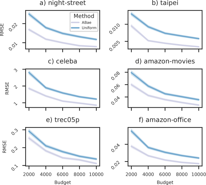
Figure 2. Sampling budget vs RMSE for uniform sampling and ABae, with the standard deviation shaded. ABae outperforms on all budgets and datasets we evaluated on. ABae can outperform by up to 1.5$\times$ on RMSE at a fixed budget and achieve the same error with up to 2$\times$ fewer samples.

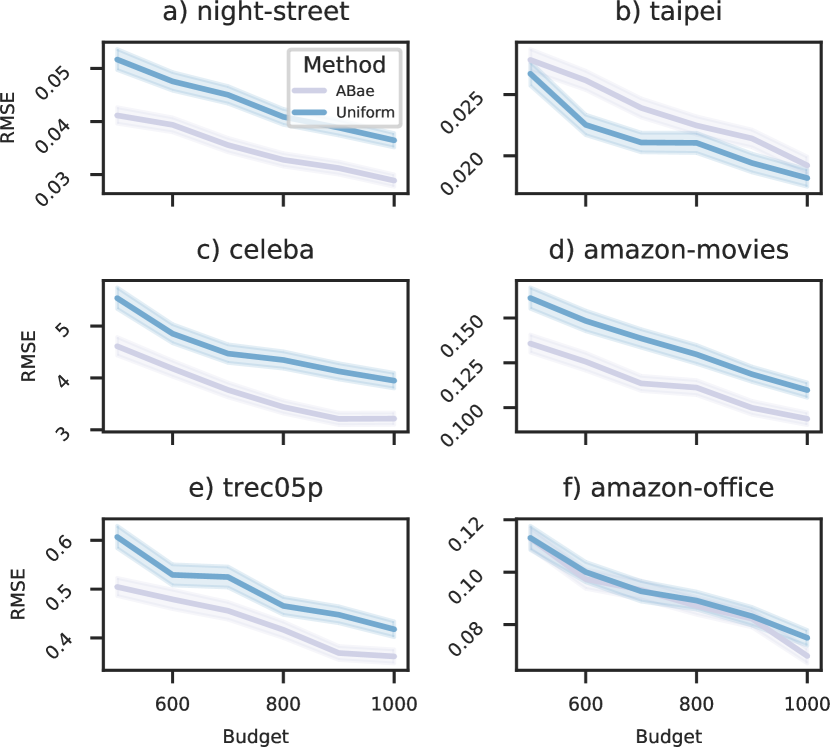
Figure 3. Low sampling budgets vs RMSE for uniform sampling and ABae, with the standard deviation shaded. We see that even at small sample sizes, ABae outperforms or matches uniform sampling in all cases.

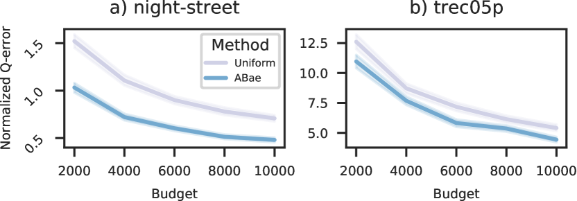
Figure 4. Sampling budget vs normalized Q-error for uniform sampling and ABae, with the standard deviation shaded. We see that ABae outperforms on Q-error. The same trends hold for all other datasets.

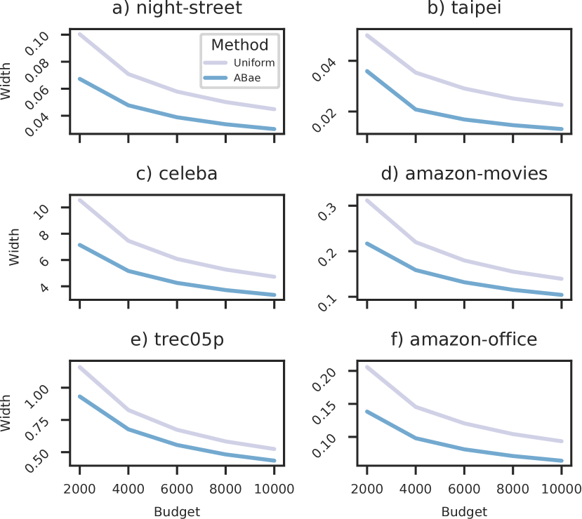
Figure 5. Sampling budget vs CI width for uniform sampling and ABae with the standard deviation of the width shaded (not visible in many plots). ABae can outperform by up to 1.5$\times$ on CI width at a fixed budget and achieve the same width with up to 2$\times$ fewer samples.

Single predicate. We show that ABae outperforms uniform sampling on the metric of RMSE. For each dataset and query, we executed ABae and random sampling for sampling budgets of 2,000 to 10,000 in increments of 2,000. We used five strata and allocated half budget to each stage. We used a failure probability of 5% for every condition. We ran every condition 1,000 times.

As shown in Figure 2, ABae outperforms for every dataset, query, and budget setting we consider. ABae can achieve up to 2.3$\times$ improvements in RMSE at a fixed budget or up to 2$\times$ fewer samples at a fixed error rate. We additionally show that ABae outperforms uniform sampling at low sampling budgets (500-1,000) in Figure 3.

We further show that ABae outperforms on Q-error (Moerkotte et al., 2009), which is a relative error metric that penalizes under- and over-estimation symmetrically. We show the normalized Q-error (i.e., $100\times(q-1)$), which roughly indicates percent error in Figure 4. As shown, ABae outperforms on the two datasets we show–ABae also outperforms on all the other datasets by 14-70%, which we omit for brevity. ABae similarly outperform on relative error by 13-76%.

We further show that ABae outperforms on the metric of confidence interval (CI) width. For each dataset and query, we executed ABae and random sampling with the parameters above. We ran every condition 1,000 times.

ABae outperforms for every dataset, query, and budget setting we consider (Figure 5). ABae can outperform by up to 1.5$\times$ on CI width at a fixed budget. Furthermore, to achieve the same confidence interval width, ABae can use up to 2$\times$ fewer samples. Finally, ABae satisfies the nominal coverage across all datasets and settings.

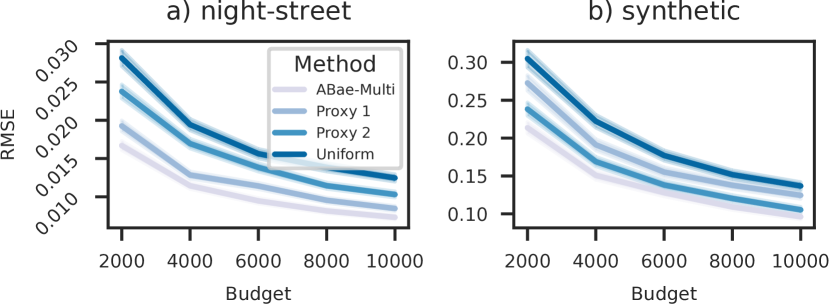
Figure 6. Sampling budget vs RMSE for uniform sampling and ABae-MultiPred, with the standard deviation shaded. As shown, ABae-MultiPred outperforms on both queries and all budgets we evaluated on.

Multiple predicates. We show that ABae-MultiPred outperforms random sampling and using a proxy for a single predicate. For the night-street dataset, we executed the following query:

⬇

SELECT AVG(count_cars(frame)) FROM video

WHERE count_cars(frame) > 0

AND red_light(frame)

The positive rate is $0.17$. We additionally executed a query on a synthetic dataset with five strata and two predicates. For each proxy, we draw the $p_{k}$ values from a Beta distribution. As shown in Figure 6, ABae-MultiPred outperforms on both queries and every budget setting we consider.

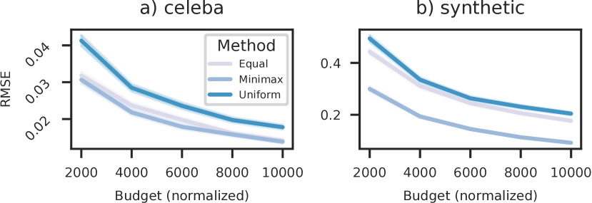
Figure 7. Normalized sampling budget vs max RMSE for uniform sampling and ABae-GroupBy with a single oracle (standard deviation shaded). ABae-GroupBy outperforms on both queries and on all budgets we evaluated on.

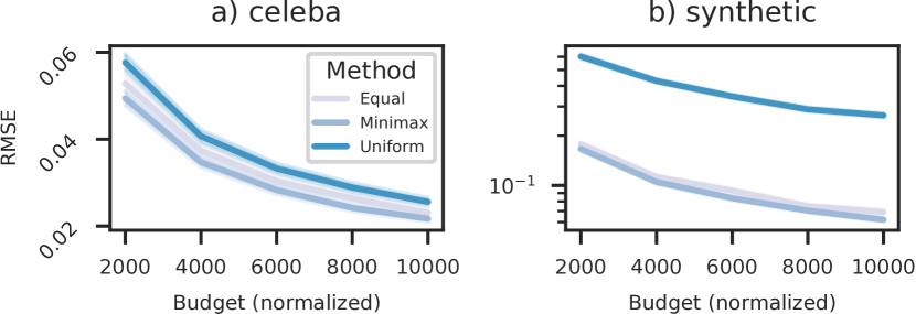
Figure 8. Normalized sampling budget vs max RMSE for uniform sampling and ABae-GroupBy with multiple, per-group oracle, with the standard deviation shaded. The y-axis is on a log-scale. The budget is normalized by the total number of groups. ABae-GroupBy outperforms on both queries and on all budgets we evaluated on.

Group bys (single oracle). We show that ABae-GroupBy outperforms random sampling in the single oracle setting. For the celeba dataset, we executed the following query:

⬇

SELECT PERCENTAGE(is_smiling(image)) FROM images

WHERE HAIR_COLOR(image) = "gray"

OR HAIR_COLOR(image) = "blond"

GROUP BY HAIR_COLOR(image)

We additionally executed a synthetic query where the statistic was distributed normally and the predicate was generated as a Bernoulli with the proxy probability. The synthetic dataset had four groups with a positive rate of 3.3%, 3.3%, 3.4%, and 3.5% respectively.

For these queries, we normalized the budget by the total number of groups. We measured the maximum RMSE over all groups. As shown in Figure 7, ABae-GroupBy outperforms on both queries and all budget settings we consider.

Group bys (multiple oracles). We show that ABae-GroupBy outperforms random sampling when a separate oracle is requires for each group by key. For the celeba dataset, we executed the same query as for group bys witn a single oracle. We additionally executed a synthetic query where the statistic was distributed normally and the predicate was generated as a Bernoulli with the proxy probability. The synthetic dataset ahd four groups with positive rates of 16%, 12%, 9%, and 5% respectively.

For these queries, we normalized the budget by the total number of groups as extracting the group key requires executing multiple models. We measured the maximum RMSE over all groups. As shown in Figure 8, ABae-GroupBy outperforms on both queries and all budget settings we consider.

Discussion of results. To contextualize our results, we first note that relative errors for some of the datasets are as high as 12% (Figure 4b). As a result, a 2$\times$ decrease in error (or number of samples at a fixed error) represents a substantial improvement. Several of our ongoing collaborations at Stanford University and elsewhere require expert human labeling as part of scientific studies. Requiring 2$\times$ fewer human labels is a substantial decrease in expert time.

5.3. Lesion and Sensitivity Analysis

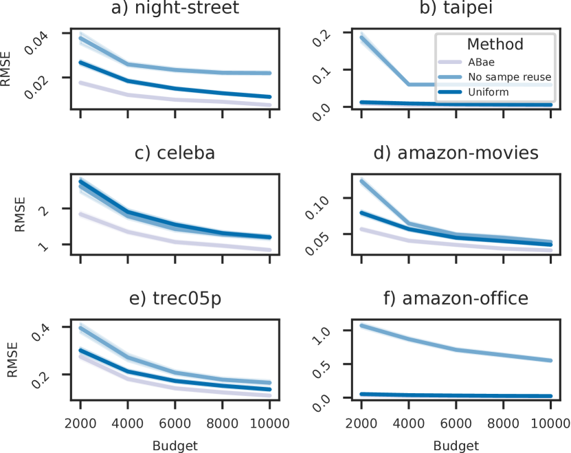
Figure 9. Lesion study when removing sample reuse and all components (i.e., uniform sampling) of ABae. As shown, both sample reuse and allocation between strata are critical for performance on all datasets.

Lesion study. We performed a lesion study in which we removed sample reuse and our two stage procedure (i.e., uniform sampling). Specifically, we executed ABae, ABae without sample reuse, and random sampling on all datasets. We used 10,000 samples for all conditions and ran 1,000 trials. For ABae, we used five strata and allocated half of the samples in each stage.

As shown in Figure 9, both parts of ABae are necessary for high performance. In particular, removing sample reuse substantially harms query performance. Sample reuse contributes to more accurate estimates of $p_{k}$, which is critical for low error.

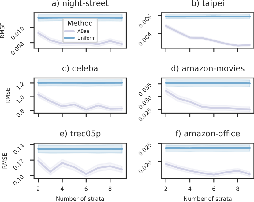
Figure 10. Sensitivity analysis of ABae to the number of strata. As shown, ABae outperforms on all values of $K$ we evaluated on compared to uniform sampling.

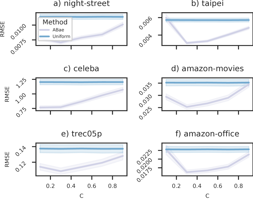
Figure 11. Sensitivity analysis of ABae to the fraction of samples between Stage 1 and Stage 2. As shown, ABae generally outperforms, except for extreme values of $C$.

Sensitivity analysis. We analyzed the sensitivity of ABae to the number of strata ($K$) and the fraction of samples between Stage 1 and Stage 2 ($C$). We executed ABae when varying $K$ and $C$ with a budget of 10,000 and ran 1,000 trials for each condition and dataset.

We varied $K$ from two to 10 and compared to uniform sampling. As shown in Figure 10, ABae outperforms on all choices of $K$ for all datasets. We find that, perhaps surprisingly, the number of strata does does not affect strongly performance relative to the performance of uniform sampling. However, in our datasets, more strata tends to perform better.

We varied $C$ from 0.1 to 0.9 in increments of 0.2. We compared to uniform sampling. As shown in Figure 11, ABae outperforms for $C$ between 0.3 and 0.7, a wide range of values. Several datasets underperform on extreme values of $C$ (0.1 and 0.9), but these are outside of our recommended values of $C$.

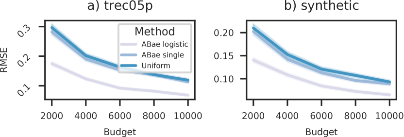
Figure 12. Uniform sampling, ABae with a single proxy, and ABae combining proxies. As shown, ABae’s method of combining proxies outperforms baselines.

Combining proxies. We analyzed if ABae’s method of combining proxies via logistic regression can improve performance. We used keyword-based proxies for the trec05p dataset and a synthetic dataset. For the synthetic dataset, we generated Bernoulli random variables and the proxies were the Bernoulli parameters with noise.

We show results for uniform sampling, single proxy ABae, and ABae with the combined proxy in Figure 12. As shown, ABae can combine proxies, effectively “ignoring” low quality proxies.

6. Related Work

AQP. A recent survey on AQP techniques categorizes AQP into offline and online methods (Li and Li, 2018). The closest work in AQP are offline methods, which use pre-computed samples (Agarwal et al., 2013; Acharya et al., 1999), histograms (Piatetsky-Shapiro and Connell, 1984; Poosala et al., 1996; Cormode et al., 2009), wavelets (Guha and Harb, 2005), and sketches (Garofalakis et al., 2002; Gan et al., 2020) to accelerate approximate queries. These techniques involve computation at ingest time to generate a synopses based on expected query workload (Li and Li, 2018), but assume the records are already present as structured data. Since we assume the predicates are expensive to compute, we cannot compute these synopses at ingest time.

ABae is also related to online methods, where the statistic is computed on the fly. For example, online aggregation provides shrinking confidence intervals as the query is executed (Hellerstein et al., 1997). These techniques also largely rely on precomputed information, e.g., indexes.

Surveying and optimal allocation. Work in the surveying and classical sampling literature have long studied stratified sampling (Scheaffer et al., 2011; Nassiuma, 2001). If the strata variances and costs are known, the optimal allocation is proportional to $\frac{\sigma_{k}}{\sqrt{c_{k}}}$, for costs $c_{k}$ (Kish, 1965). The closest work we are aware of are algorithms for stratified sampling where the strata variances are not known (Carpentier et al., 2015; Arouna, 2004). This work does not consider the case of stochastic draws, as we do.

Other work in surveying considers stratified sampling with non-responses, such as non-responses to mail surveys (Hansen and Hurwitz, 1946). This literature is largely concerned with estimating the bias from non-responses or focusing on which subpopulations to follow up with, e.g., with phone calls (Khan et al., 2008; Filion, 1975; Varshney et al., 2012). In this work, not all of the population satisfies the predicate, so the non-response model is different.

A common technique in scientific studies and surveying is pilot sampling, in which a small sample is used for preliminary analysis. Pilot sampling is commonly used in randomized trials (Thabane et al., 2010) and to estimate various quantities for downstream sampling (strata variances, sampling costs, feasibility, etc.) (Kish, 1965; Denne and Jennison, 1999; Eldridge et al., 2016; Cochran, 2007). In our setting, each sample has a stochastic probability of giving useful information instead of a cost, which is not covered by prior work. However, the allocations in ABae coincide with those made by defining hypothetical costs proportional to $\frac{1}{p_{k}}$. To show that this allocation remains valid in our setting, we prove that Stage 1 of ABae is optimal with high probability, something which is not handled by standard survey sampling theory.

Stratified sampling in data management systems. Several traditional systems and algorithms use stratified sampling to accelerate sampling (Agarwal et al., 2013; Acharya et al., 1999; Chaudhuri et al., 2007). In the data management literature, using stratified sampling typically requires pre-computation, which is not applicable for the same reasons as described above.

Recent work learns machine learning models, such as classification DNNs or generative adversarial networks (GANs), over relational data to improve AQP (Li, 2020; Thirumuruganathan et al., 2020; Walenz et al., 2019). These approaches approximate the data (e.g., the result of a predicate or overall data statistics), which can be faster than directly accessing the data. However, they do not apply to complex unstructured data sources that we consider in this work.

Proxies. Recent work has focused on accelerated DNN-based queries by using proxies. Many systems have been developed to accelerate certain classes of queries using proxies, including selection without statistical guarantees (Kang et al., 2017; Lu et al., 2018; Anderson et al., 2019; Hsieh et al., 2018), selection with statistical guarantees (Kang et al., 2020a), aggregation queries without predicates (Kang et al., 2019), and limit queries (Kang et al., 2019). The work on selection does not directly apply to our setting, since these systems do not guarantee that the records selected are independent of the statistic we wish to compute. The BlazeIt system accelerates aggregation queries over the entire dataset by using proxies as a control variate, but does not consider aggregation queries with predicates (Kang et al., 2019). We add to this body of literature by designing an algorithm for stochastic draws to address that many aggregation queries contain predicates.

DNN-based queries. Other work aims to accelerate other DNN-based queries. Several systems aim to improve execution speeds or latency of DNNs on accelerators (Zhang et al., 2017; Poms et al., 2018; Kang et al., 2021b), which are complementary to our work. Other work assumes that the target DNN is not expensive to execute or that extracting bounding boxes is not expensive (Zhang and Kumar, 2019; Fu et al., 2019). We have found that many applications require accurate and expensive target DNNs, so we focus on reducing executing the target DNN via sampling.

7. Conclusion

To reduce the cost of approximate aggregation queries with expensive predicates, we introduce stratified sampling algorithms leveraging proxies. We provide proofs of convergence for stratified sampling with stochastic draws, which corresponds to our setting. We show that ABae achieves optimal rates. We further extend ABae to answer queries with multiple predicates and group by keys. We show that our algorithms outperform baselines by up to 2.3$\times$ on a wide range of domains and predicates.

- (1)
- Acharya et al. (1999) Swarup Acharya, Phillip B Gibbons, and Viswanath Poosala. 1999. Aqua: A fast decision support systems using approximate query answers. In PVLDB. 754–757.
- Agarwal et al. (2013) Sameer Agarwal, Barzan Mozafari, Aurojit Panda, Henry Milner, Samuel Madden, and Ion Stoica. 2013. BlinkDB: queries with bounded errors and bounded response times on very large data. In EuroSys. ACM, 29–42.
- Akbik et al. (2018) Alan Akbik, Duncan Blythe, and Roland Vollgraf. 2018. Contextual String Embeddings for Sequence Labeling. In COLING 2018, 27th International Conference on Computational Linguistics. 1638–1649.
- Anderson et al. (2019) Michael R Anderson, Michael Cafarella, Thomas F Wenisch, and German Ros. 2019. Predicate Optimization for a Visual Analytics Database. ICDE (2019).
- Arouna (2004) Bouhari Arouna. 2004. Adaptative Monte Carlo method, a variance reduction technique. (2004).
- Boyd et al. (2004) Stephen Boyd, Stephen P Boyd, and Lieven Vandenberghe. 2004. Convex optimization. Cambridge university press.
- Braverman and Ostrovsky (2013) Vladimir Braverman and Rafail Ostrovsky. 2013. Generalizing the layering method of indyk and woodruff: Recursive sketches for frequency-based vectors on streams. In Approximation, Randomization, and Combinatorial Optimization. Algorithms and Techniques. Springer, 58–70.
- Canel et al. (2019) Christopher Canel, Thomas Kim, Giulio Zhou, Conglong Li, Hyeontaek Lim, David Andersen, Michael Kaminsky, and Subramanya Dulloor. 2019. Scaling Video Analytics on Constrained Edge Nodes. SysML (2019).
- Carpentier et al. (2015) Alexandra Carpentier, Remi Munos, and András Antos. 2015. Adaptive strategy for stratified Monte Carlo sampling. J. Mach. Learn. Res. 16 (2015), 2231–2271.
- Chaudhuri et al. (2007) Surajit Chaudhuri, Gautam Das, and Vivek Narasayya. 2007. Optimized stratified sampling for approximate query processing. TODS (2007).
- Chung and Lu (2002) Fan Chung and Linyuan Lu. 2002. Connected components in random graphs with given expected degree sequences. Annals of combinatorics 6, 2 (2002), 125–145.
- Cochran (2007) William G Cochran. 2007. Sampling techniques. John Wiley & Sons.
- Cormack and Lynam (2005) Gordon V Cormack and Thomas R Lynam. 2005. TREC 2005 Spam Track Overview.. In TREC. 500–274.
- Cormode et al. (2009) Graham Cormode, Antonios Deligiannakis, Minos Garofalakis, and Andrew McGregor. 2009. Probabilistic histograms for probabilistic data. Proceedings of the VLDB Endowment 2, 1 (2009), 526–537.
- Denne and Jennison (1999) Jonathan S Denne and Christopher Jennison. 1999. Estimating the sample size for at-test using an internal pilot. Statistics in Medicine 18, 13 (1999), 1575–1585.
- Efron and Tibshirani (1994) Bradley Efron and Robert J Tibshirani. 1994. An introduction to the bootstrap. CRC press.
- Eldridge et al. (2016) Sandra M Eldridge, Gillian A Lancaster, Michael J Campbell, Lehana Thabane, Sally Hopewell, Claire L Coleman, and Christine M Bond. 2016. Defining feasibility and pilot studies in preparation for randomised controlled trials: development of a conceptual framework. PloS one 11, 3 (2016), e0150205.
- Filion (1975) FL Filion. 1975. Estimating bias due to nonresponse in mail surveys. Public Opinion Quarterly 39, 4 (1975), 482–492.
- Fu et al. (2019) Daniel Y Fu, Will Crichton, James Hong, Xinwei Yao, Haotian Zhang, Anh Truong, Avanika Narayan, Maneesh Agrawala, Christopher Ré, and Kayvon Fatahalian. 2019. Rekall: Specifying video events using compositions of spatiotemporal labels. arXiv preprint arXiv:1910.02993 (2019).
- Gan et al. (2020) Edward Gan, Peter Bailis, and Moses Charikar. 2020. Coopstore: Optimizing precomputed summaries for aggregation. Proceedings of the VLDB Endowment 13, 12 (2020), 2174–2187.
- Garofalakis et al. (2002) Minos Garofalakis, Johannes Gehrke, and Rajeev Rastogi. 2002. Querying and mining data streams: you only get one look a tutorial. In Proceedings of the 2002 ACM SIGMOD international conference on Management of data. 635–635.
- Guha and Harb (2005) Sudipto Guha and Boulos Harb. 2005. Wavelet synopsis for data streams: minimizing non-euclidean error. In Proceedings of the eleventh ACM SIGKDD international conference on Knowledge discovery in data mining. 88–97.
- Guo et al. (2017) Chuan Guo, Geoff Pleiss, Yu Sun, and Kilian Q Weinberger. 2017. On calibration of modern neural networks. In International Conference on Machine Learning. PMLR, 1321–1330.
- Hansen and Hurwitz (1946) Morris H Hansen and William N Hurwitz. 1946. The problem of non-response in sample surveys. J. Amer. Statist. Assoc. 41, 236 (1946), 517–529.
- Hartung et al. (2011) Joachim Hartung, Guido Knapp, and Bimal K Sinha. 2011. Statistical meta-analysis with applications. Vol. 738. John Wiley & Sons.
- He et al. (2017) Kaiming He, Georgia Gkioxari, Piotr Dollár, and Ross Girshick. 2017. Mask r-cnn. In ICCV. IEEE, 2980–2988.
- Hellerstein et al. (1997) Joseph M Hellerstein, Peter J Haas, and Helen J Wang. 1997. Online aggregation. In Acm Sigmod Record, Vol. 26. ACM, 171–182.
- Hong et al. (2020) James Hong, Will Crichton, Haotian Zhang, Daniel Y Fu, Jacob Ritchie, Jeremy Barenholtz, Ben Hannel, Xinwei Yao, Michaela Murray, Geraldine Moriba, et al. 2020. Analyzing Who and What Appears in a Decade of US Cable TV News. arXiv preprint arXiv:2008.06007 (2020).
- Hsieh et al. (2018) Kevin Hsieh, Ganesh Ananthanarayanan, Peter Bodik, Paramvir Bahl, Matthai Philipose, Phillip B Gibbons, and Onur Mutlu. 2018. Focus: Querying Large Video Datasets with Low Latency and Low Cost. OSDI (2018).
- Hutto and Gilbert (2014) Clayton Hutto and Eric Gilbert. 2014. Vader: A parsimonious rule-based model for sentiment analysis of social media text. In Proceedings of the International AAAI Conference on Web and Social Media, Vol. 8.
- Jiang et al. (2018) Junchen Jiang, Ganesh Ananthanarayanan, Peter Bodik, Siddhartha Sen, and Ion Stoica. 2018. Chameleon: scalable adaptation of video analytics. In Proceedings of the 2018 Conference of the ACM Special Interest Group on Data Communication. ACM, 253–266.
- Kang et al. (2019) Daniel Kang, Peter Bailis, and Matei Zaharia. 2019. BlazeIt: Optimizing Declarative Aggregation and Limit Queries for Neural Network-Based Video Analytics. PVLDB (2019).
- Kang et al. (2017) Daniel Kang, John Emmons, Firas Abuzaid, Peter Bailis, and Matei Zaharia. 2017. NoScope: optimizing neural network queries over video at scale. PVLDB 10, 11 (2017), 1586–1597.
- Kang et al. (2020a) Daniel Kang, Edward Gan, Peter Bailis, Tatsunori Hashimoto, and Matei Zaharia. 2020a. Approximate Selection with Guarantees using Proxies. PVLDB (2020).
- Kang et al. (2020b) Daniel Kang, John Guibas, Peter Bailis, Tatsunori Hashimoto, and Matei Zaharia. 2020b. Task-agnostic Indexes for Deep Learning-based Queries over Unstructured Data. arXiv preprint arXiv:2009.04540 (2020).
- Kang et al. (2021a) Daniel Kang, John Guibas, Peter Bailis, Yi Sun, Tatsunori Hashimoto, and Matei Zaharia. 2021a. Proof: Accelerating Approximate Aggregation Queries with Expensive Predicates. arXiv preprint arXiv:2107.12525 (2021).
- Kang et al. (2021b) Daniel Kang, Ankit Mathur, Teja Veeramacheneni, Peter Bailis, and Matei Zaharia. 2021b. Jointly optimizing preprocessing and inference for DNN-based visual analytics. PVLDB (2021).
- Khan et al. (2008) Mohammad GM Khan, EA Khan, and MJ Ahsan. 2008. Optimum allocation in multivariate stratified sampling in presence of non-response. Journal of the Indian Society of Agricultural Statistics 62, 1 (2008), 42–48.
- Kish (1965) Leslie Kish. 1965. Survey sampling. Number 04; HN29, K5.
- Li and Li (2018) Kaiyu Li and Guoliang Li. 2018. Approximate query processing: What is new and where to go? Data Science and Engineering 3, 4 (2018), 379–397.
- Li (2020) Wanxin Li. 2020. Supporting Database Constraints in Synthetic Data Generation based on Generative Adversarial Networks. In Proceedings of the 2020 ACM SIGMOD International Conference on Management of Data. 2875–2877.
- Liu et al. (2015) Ziwei Liu, Ping Luo, Xiaogang Wang, and Xiaoou Tang. 2015. Deep Learning Face Attributes in the Wild. In Proceedings of International Conference on Computer Vision (ICCV).
- Lu et al. (2018) Yao Lu, Aakanksha Chowdhery, Srikanth Kandula, and Surajit Chaudhuri. 2018. Accelerating Machine Learning Inference with Probabilistic Predicates. In SIGMOD. ACM, 1493–1508.
- Moerkotte et al. (2009) Guido Moerkotte, Thomas Neumann, and Gabriele Steidl. 2009. Preventing bad plans by bounding the impact of cardinality estimation errors. Proceedings of the VLDB Endowment 2, 1 (2009), 982–993.
- Nassiuma (2001) Dankit K Nassiuma. 2001. Survey sampling: Theory and methods.
- Ni et al. (2019) Jianmo Ni, Jiacheng Li, and Julian McAuley. 2019. Justifying recommendations using distantly-labeled reviews and fine-grained aspects. In Proceedings of the 2019 Conference on Empirical Methods in Natural Language Processing and the 9th International Joint Conference on Natural Language Processing (EMNLP-IJCNLP). 188–197.
- Piatetsky-Shapiro and Connell (1984) Gregory Piatetsky-Shapiro and Charles Connell. 1984. Accurate estimation of the number of tuples satisfying a condition. SIGMOD (1984).
- Poms et al. (2018) Alex Poms, William Crichton, Pat Hanrahan, and Kayvon Fatahalian. 2018. Scanner: Efficient Video Analysis at Scale (To Appear). (2018).
- Poosala et al. (1996) Viswanath Poosala, Peter J Haas, Yannis E Ioannidis, and Eugene J Shekita. 1996. Improved histograms for selectivity estimation of range predicates. ACM Sigmod Record 25, 2 (1996), 294–305.
- Sandler et al. (2018) Mark Sandler, Andrew Howard, Menglong Zhu, Andrey Zhmoginov, and Liang-Chieh Chen. 2018. Mobilenetv2: Inverted residuals and linear bottlenecks. In Proceedings of the IEEE conference on computer vision and pattern recognition. 4510–4520.
- Scheaffer et al. (2011) Richard L Scheaffer, William Mendenhall III, R Lyman Ott, and Kenneth G Gerow. 2011. Elementary survey sampling. Cengage Learning.
- Serengil and Ozpinar (2020) Sefik Ilkin Serengil and Alper Ozpinar. 2020. LightFace: A Hybrid Deep Face Recognition Framework. In 2020 Innovations in Intelligent Systems and Applications Conference (ASYU). IEEE, 23–27. https://doi.org/10.1109/ASYU50717.2020.9259802
- Sorensen (1982) Danny C Sorensen. 1982. Newton’s method with a model trust region modification. SIAM J. Numer. Anal. 19, 2 (1982), 409–426.
- Tarjan (2009) Robert Tarjan. 2009. 15-359: Probability and Computing Lecture 10: More Chernoff Bounds, Sampling, and the Chernoff + Union Bound method. http://aiweb.techfak.uni-bielefeld.de/content/bworld-robot-control-software/. [Online; accessed 11-Feb-2021].
- Thabane et al. (2010) Lehana Thabane, Jinhui Ma, Rong Chu, Ji Cheng, Afisi Ismaila, Lorena P Rios, Reid Robson, Marroon Thabane, Lora Giangregorio, and Charles H Goldsmith. 2010. A tutorial on pilot studies: the what, why and how. BMC medical research methodology 10, 1 (2010), 1–10.
- Thirumuruganathan et al. (2020) Saravanan Thirumuruganathan, Shohedul Hasan, Nick Koudas, and Gautam Das. 2020. Approximate query processing for data exploration using deep generative models. In 2020 IEEE 36th International Conference on Data Engineering (ICDE). IEEE, 1309–1320.
- Varshney et al. (2012) Rahul Varshney, MJ Ahsan, et al. 2012. An optimum multivariate stratified double sampling design in presence of non-response. Optimization Letters 6, 5 (2012), 993–1008.
- Walenz et al. (2019) Brett Walenz, Stavros Sintos, Sudeepa Roy, and Jun Yang. 2019. Learning to sample: Counting with complex queries. arXiv preprint arXiv:1906.09335 (2019).
- Xu et al. (2019) Tiantu Xu, Luis Materon Botelho, and Felix Xiaozhu Lin. 2019. VStore: A Data Store for Analytics on Large Videos. In Proceedings of the Fourteenth EuroSys Conference 2019. ACM, 16.
- Zhang et al. (2018) Changzheng Zhang, Xiang Xu, and Dandan Tu. 2018. Face detection using improved faster rcnn. arXiv preprint arXiv:1802.02142 (2018).
- Zhang et al. (2017) Haoyu Zhang, Ganesh Ananthanarayanan, Peter Bodik, Matthai Philipose, Paramvir Bahl, and Michael J Freedman. 2017. Live Video Analytics at Scale with Approximation and Delay-Tolerance. In NSDI, Vol. 9. 1.
- Zhang et al. (2016) Kaipeng Zhang, Zhanpeng Zhang, Zhifeng Li, and Yu Qiao. 2016. Joint face detection and alignment using multitask cascaded convolutional networks. IEEE Signal Processing Letters 23, 10 (2016), 1499–1503.
- Zhang and Kumar (2019) Yuhao Zhang and Arun Kumar. 2019. Panorama: a data system for unbounded vocabulary querying over video. Proceedings of the VLDB Endowment 13, 4 (2019), 477–491.