Dark energy interactions near the galactic centre
Abstract
We investigate scalar-tensor theories, motivated by dark energy models, in the strong gravity regime around the black hole at the centre of our galaxy. In such theories general relativity is modified since the scalar field couples to matter. We consider the most general conformal and disformal couplings of the scalar field to matter to study the orbital behaviour of the nearby stars around the galactic star center . Markov Chain Monte Carlo (MCMC) simulation yields a bound on the parameters of the couplings of the scalar field to matter. Using Bayesian Analysis yields the first constraints on such theories in the strong gravity regime.
I Introduction
The discovery that the Universe is undergoing a period of accelerated expansion today requires a modification of General Relativity (GR). This could be the addition of a Cosmological Constant , Perlmutter et al. (1999); Weinberg (1989); Lombriser (2019); Copeland et al. (2006); Frieman et al. (2008); Riess et al. (2019). This, however, requires severe fine tuning by and is viewed as theoretically unsatisfactory. Another theoretical mechanism developed is the quintessence model Starobinsky (1979, 1980); Guth (1981); Albrecht and Steinhardt (1982); Mukhanov and Chibisov (1981); Guth and Pi (1982); Linde (1982); Barrow and Cotsakis (1988); Barrow (1988); Elizalde et al. (2008); Ratra and Peebles (1988); Caldwell et al. (1998); Zlatev et al. (1999); Caldwell (2002); Chiba et al. (2000); Bento et al. (2002); Tsujikawa (2013); Caldwell et al. (1998); Ratra and Peebles (1988); Peebles and Ratra (1988); Barreiro et al. (2000); Carroll (1998); Chiba (1999); Sahni and Wang (2000), where a scalar field with a slow roll behaviour is responsible for the late time acceleration of our universe. In such models the scalar field does not couple to ordinary matter, either directly or by quantum corrections. Other possibilities include a modification of general relativity itself. Such possibilities include modifying the Einstein-Hilbert action to become a function of the Ricci scalar, the so-called f(R) theories, or the addition of a scalar field which couples to matter, the scalar-tensor theories. The coupling between the scalar field and matter is derived using theoretical considerations, involving a transformation from Jordan to Einstein frames, see Saridakis et al. (2021) for a recent review. Bekenstein has shown the most general coupling of a scalar field to matter is via a conformal and disformal transformation Bekenstein (1993). Scalar-tensor theories with a conformal coupling can be rewritten in terms of and vice versa Brax et al. (2008). However, such theories give rise to fifth forces which are subject to strict limits by solar system tests of general relativity Bertotti et al. (2003). Consequently the effect of fifth forces need to be screened in the solar system, giving rise to screened modified gravity models whereby the effects of the scalar field depends on the environment. Such models can be screened via the chameleon mechanism Khoury and Weltman (2004); Brax et al. (2004), symmetron Hinterbichler and Khoury (2010), Vainshtein Vainshtein (1972) or Damour-Polyakov mechanism Damour and Polyakov (1994); Brax et al. (2010). All rely in different respects on the environment such that the fifth force is screened in the solar system and the theory evades all solar system tests but can give rise to modifications to GR on cosmological scales Damour and Esposito-Farese (1992); Julié and Deruelle (2017); Bertotti et al. (2003); Williams et al. (2004); Khoury and Weltman (2004); Damour and Polyakov (1994); Vainshtein (1972); Babichev et al. (2009).
Similarly the disformal coupling to matter gives rise to modifications to GR which can be constrained in the solar systemBrax and Davis (2018) and in collider physicsBrax et al. (2015). This results in constraints on the disformal coupling to matter. Koivisto (2008); Zumalacarregui et al. (2010); Koivisto et al. (2012); van de Bruck et al. (2013); Brax et al. (2013); Neveu et al. (2014); Sakstein (2014, 2015); Desmond et al. (2019).
Whilst solar system physics puts constraints on any modified gravity model theories with screening can still give observational effects. For example whilst the fifth force is suppressed in the solar system they give rise to deviations on cosmological scales from the standard GR predictions and could modify the growth of structures. Such deviations could be detected in future satellite experiments Vagnozzi et al. (2021); Brax et al. (2020a).
It is also possible to constrain a class of modified gravity models, namely those that screen with the chameleon Yoo and Watanabe (2012); Karwal et al. (2021) or symmetron mechanism Hinterbichler et al. (2011), using laboratory experiments Brax et al. (2018); Elder et al. (2020); Brax et al. (2020b, a). Indeed such experiments give tight constraints on the model parameters. This means that this class of models are constrained by observation on very different scales and different regimes.
Whilst modified gravity models have been tested on both small and solar system scales and their effects on cosmology computed in some cases they have yet to be tested in the strong gravity regime. This is the goal of our work. It is known that there is a relativistic, compact object in the galactic centre; the black hole . The stars orbiting are called the S-starsYu et al. (2016); Boehle et al. (2016); Abuter et al. (2018); Gillessen et al. (2009); Do et al. (2019); Abuter et al. (2020); Amorim et al. (2019); Parsa et al. (2017). A large fraction of these stars have orbits with high eccentricities. Thus, they reach high velocities at the pericenter and can be used for constraining modified gravity Will (2018, 1998); Scharre and Will (2002); Moffat (2006); Zhao and Tian (2006); Bailey and Kostelecky (2006); Deng et al. (2009); Barausse et al. (2013); Borka et al. (2012); Enqvist et al. (2013); Borka et al. (2013); Capozziello et al. (2014); Berti et al. (2015); Borka et al. (2016); Zakharov et al. (2016); Zhang et al. (2017); Dirkes (2018); Pittordis and Sutherland (2018); Hou and Gong (2018); Nakamura et al. (2019); Banik and Zhao (2018); Dialektopoulos et al. (2019); Kalita (2018); Will (2018); Banik (2019); Pittordis and Sutherland (2019); Nunes et al. (2019); Anderson et al. (2019); Gainutdinov (2020); Bahamonde et al. (2020); Banerjee et al. (2021); Ruggiero and Iorio (2020); Okcu and Aydiner (2021); de Martino et al. (2021); Della Monica et al. (2021); D’Addio et al. (2021).
Recently Brax and Davis (2018) have extended the programme of Damour and Deruelle (1985a) to include both conformal and disformal couplings to matter in scalar-tensor theories. Rather than specialising to a specific model the programme uses a general scalar-tensor theory with parameters chosen to evade known constraints and computes physical quantities using a PN expansion. This enables such theories to be tested in new regimes. Whilst previous work has concentrated on considering such theories in the solar system in this work we extend the tests to the strong gravity regime around the region of .
II Formalism
Many modified gravity models can be written in the schematic form:
| (1) |
where the scalar field . Bekenstein (1993) shows that the most general theory of a scalar coupled to matter:
| (2) |
The matter fields are denoted by and their Lagrangian is . Brax and Davis (2018) focuses of nearly massless scalar and takes the form since dark energy, which is negligible in the galactic star centre system. As a simple anzats the conformal factor is studied:
| (3) |
that is characterised by the constant coupling and the disformal interaction is specified by the suppression scale . Brax et al. (2014); Brax and Davis (2018); Kuntz (2019) use the center of mass coordinates, with the reduced mass and the total mass of the binary system . The reduced action per reads:
| (4) |
where:
| (5a) | |||
| (5b) | |||
| (5c) |
The action is to leading order in the first Post Newtonain (PN) order. When and go to zero the action reduces to the standard Einstein-Infeld-Hoffmann (EIH) action Damour and Deruelle (1985b); Blanchet (2011). The center of mass coordinate system is defined by:
| (6) |
with . Since the research focuses on the galactic star center, we set which demonstrates that the masses of the S stars is much lower then the mass of the black hole.
The variation with respect to yields:
| (7) |
with the contributing of the conformal coupling :
| (8) |
and the contribution of the disformal coupling :
| (9) |
The same equation is satisfied for the axis, with the exchange of into and vice versa:
| (10) |
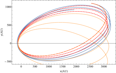
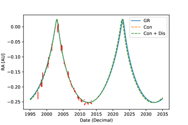
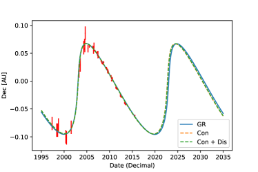
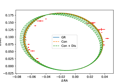
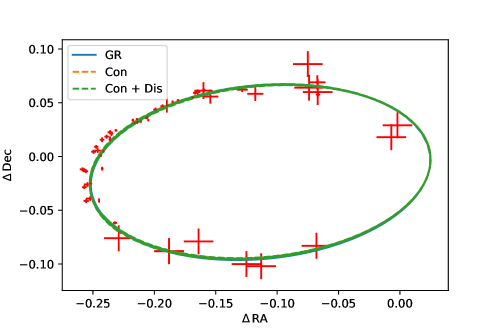
Again, when and go to zero the equation of motion reduces to the standard GR solution in the first PN limit. In order to demonstrate the effect of the conformal and the disformal transformations on the S2 motion, we solve Eq. (7) numerically. Fig 1 shows the numerical solution of the S2 orbit in the reference frame, where the location of is . The numerical solution is for 30 years. With large conformal interaction (dashed red line) and with large disformal interaction strengths, where , the procession is much bigger. Therefore the possible range for these term has to be much lower as we will see from the Bayesian Analysis.
III Methodology
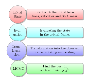
We start the first iteration using a sampling of the initial position and velocity of the corresponding star in the orbital plane at the epoch at . The true positions and velocities at all successive observed epochs are then calculated by numerical integration of equations of motion (7), and projected into the corresponding positions in the observed plane (apparent orbit). There are three angles that we take into account: is longitude of the ascending node, is longitude of pericenter and is the inclination. The transformation from the reference frame to our frame is via the rotation matrix:
| (11) |
where the expressions for and depend on three orbital elements:
We divided the location by the distance and rescaling the angle to to be consistent with the observations obtained. We perform a Bayesian statistical analysis to constrain the four chameleon, or indeed general scalar-tensor theory, parameters, which we collectively denote by . The function entering the likelihood is given by
| (12) |
Our analysis uses publicly available astrometric and spectroscopic data that have been collected during the past thirty years. We use astrometric positions spanning a period from 1992.225 to 2016.38 from Gillessen et al. (2017). The data come from speckle camera SHARP at the ESO New Technology Telescope Hofmann et al. (1993), measurements were made using the Very Large Telescope (VLT) Adaptive Optics (AO).

| Parameter | GR S2 | Con S2 | Con + Dis S2 | GR S2 S38 | Con S2 S38 | Con + Dis S2 S38 |
|---|---|---|---|---|---|---|
| - | - | |||||
| - | - | - | - | |||
| - | -3.90 | 1.70 | - | -2.41 | -1.60 |
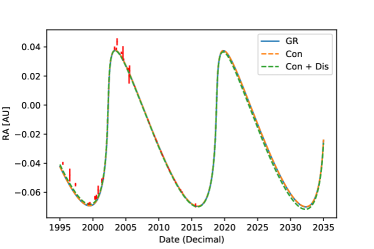
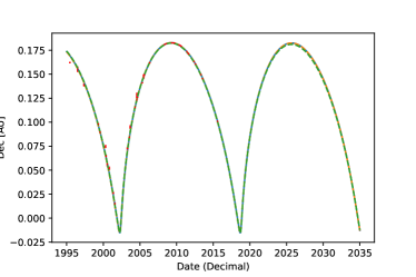
Regarding the problem of likelihood maximization, we use an affine-invariant Markov Chain Monte Carlo sampler Foreman-Mackey et al. (2013), as it is implemented within the open-source packaged Polychord Handley et al. (2015) with the GetDist package Lewis (2019) to present the results. We test three different models: the GR solution, with conformal transformation and with the disformal transformation. We test these models with respect to the measurements of the S2 and the S38 stars. The S2 and S38 stars are the closest stars orbiting and the stars for which we have data.
In order to ensure that the conformal and the disformal coupling are subdominant, we choose the corresponding prior for our fit: and for the conformal and the disformal strengths. Besides we use a unifrom prior on the distance towards the galactic center and the mass of as and . For simplicity we use the angles that reported by the Gravity collaboration as a Gaussian prior. For the rest we assume a uniform prior of the initial location and velocities.
IV Results
The posterior distribution of the S2 star fit is presented in the upper panel of 1 and the posterior distribution for the fit of the combined data of S2 and S38 is presented in the lower panel.
The obtained mass of the is changed a bit with the S38 measurements: from for GR, for the confromal interaction and with the disformal interaction, into for GR, for the conformal interaction with the disformal interaction. The distance towards is a bit decreases: from for GR, for the conformal interaction and with the disformal interaction, into for GR, for the conformal interaction .
The constraint on the conformal interaction parameter is around : for the S2 star and for the combined with S38 star. Including the disformal interaction yields for the S2 star and for the combined stars. The case of goes to zero is the GR case, however this value is outside of the mean value. This gives potential support for that this additional interaction to exist. The constraint on the disformal interaction parameter is around : for the S2 star and for S2 combined with S38 star. The case of goes to infinity is the GR case.
Finally, we can further quantify the relative ability of the conformal and the disformal interactions model to describe the various data sets w.r.t. the GR cosmology using the Bayes ratio. Given a data set , the probability of a certain model to be the best one among a given set of models reads,
| (13) |
where is the prior probability of the model and the probability of having the data set , with the normalization condition . The quantity is the so-called marginal likelihood or evidence. If the model has parameters , the evidence reads,
| (14) |
with being the likelihood and the prior of the parameters entering the model . If we compare the models by assuming equal prior probability for both of them, then we find that the ratio of their associated probabilities is directly given by the ratio of their corresponding evidences, i.e.
| (15) |
This is known as Bayes ratio and is the quantity we are interested in Kass and Raftery (1995). In order to complete the analysis we compare the BE of the models we use the values from the Polychord. The BE values are summarized in fig 1. In the first case we take only the S2 measurements. The difference between the BE of the GR case and the conformal model is and the difference between the BE of the GR case and the conformal and the disformal model is . Therefore the is a slight preference for GR vs. the conformal coupling, and an indistinguishable preference for conformal with the disformal coupling vs. GR. In the second case that we test S2 with the S38 stars The difference between the BE of the GR case and the conformal model is and the difference between the BE of the GR case and the conformal and the disformal model is . Combining the observations of the S38 star yields a slight preference for GR.
V Combined Constraints
In order to complete our discussion on the interactions in two body motion, we add the solar system constraint Ip et al. (2015). Brax and Davis (2018) gives the precession term for the conformal and the disformal contribution as:
| (16) |
Correspondingly, the from some object reads:
| (17) |
We include the precession data of the solar system from 111https://nssdc.gsfc.nasa.gov/planetary/factsheet/. The combined constraint is approached by using the combined likelihood:
| (18) |
where and include the measurements from the galactic star centre and include the precession measurements from the solar system.
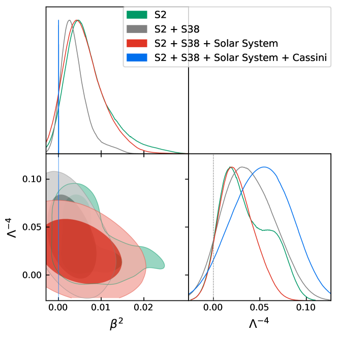
The last bound that we take into account is the Cassini bound Bertotti et al. (2003). Cassini gives a bound of for the parameter without any special bound on . In order to include the Cassini bound, we use a smaller prior on .
Fig. (7) shows the combined analysis for the conformal and the disformal couplings for different cases. The table below summarizes the final values. We see that adding the solar system constraints, without Cassini, gives very little changer to the modified gravity parameters. However, adding the Cassini bound reduces the final value of into and the value of into which is .
| Parameter | S2 + S38 + Solar System | S2 + S38 + Solar System + Cassini |
|---|---|---|
VI Discussion
We have investigated modified gravity theories in the strong gravity regime near the galactic centre using the observations of the S2 and S38 stars. To our knowledge this is the first time such theories have been investigated in the strong gravity regime. The modified gravity scalar field is both conformally and disformally coupled to matter and the observations allow both types of interaction to be constrained. Our formalism is very general using a PN expansion. As noted previously, the disformal coupling has an effect only when it combines with a conformal interaction. In this case, the disformal coupling leads to a change in the advance of perihelion for a light body and modifies the effective metric which governs the evolution of two interacting bodies. The orbital measurements around the galactic star centre , in particular the locations and the velocities of the S2 and the S38 stars, is used in our constraints. Using a MCMC simulation yields a bound on the parameters, and of the modified gravity theory. In our analysis we note that the BE gives a slight preference for GR.
The bound on the conformal and disformal couplings from different systems is widely constrained. Such a range for is constrained from the Eotwash experiment with the lower bound of and from the Cassini experiment Bertotti et al. (2003). The posterior distribution for is about and the bound of yields a range of . The bounds we have obtained from the galactic star centre with the Cassini experiments gives a strong statement on the interactions of DE in the strong gravity regime of the galactic centre.
In future it would be interesting to add other cosmological measurements such from those arising from the expansion history of the Universe and structure formation data. The cosmological data require more specific form of potentials and conformal and disformal couplings in order to make a complete combined analysis. Such analysis is left for future work.
Acknowledgements.
We thank Wyn Evans, Eduardo I. Guendelman, Salvatore Cappoziello and Philippe Brax for discussions and insightful comments. D.B gratefully acknowledge the support from the Blavatnik and the Rothschild fellowships. We have received partial support from European COST actions CA15117 and CA18108 and STFC consolidated grants ST/P0006811 and ST/T0006941.References
- Perlmutter et al. (1999) S. Perlmutter et al. (Supernova Cosmology Project), Astrophys. J. 517, 565 (1999), arXiv:astro-ph/9812133 [astro-ph] .
- Weinberg (1989) S. Weinberg, Rev. Mod. Phys. 61, 1 (1989), [,569(1988)].
- Lombriser (2019) L. Lombriser, Phys. Lett. B797, 134804 (2019), arXiv:1901.08588 [gr-qc] .
- Copeland et al. (2006) E. J. Copeland, M. Sami, and S. Tsujikawa, Int. J. Mod. Phys. D 15, 1753 (2006), arXiv:hep-th/0603057 .
- Frieman et al. (2008) J. Frieman, M. Turner, and D. Huterer, Ann. Rev. Astron. Astrophys. 46, 385 (2008), arXiv:0803.0982 [astro-ph] .
- Riess et al. (2019) A. G. Riess, S. Casertano, W. Yuan, L. M. Macri, and D. Scolnic, Astrophys. J. 876, 85 (2019), arXiv:1903.07603 [astro-ph.CO] .
- Starobinsky (1979) A. A. Starobinsky, JETP Lett. 30, 682 (1979), [,767(1979)].
- Starobinsky (1980) A. A. Starobinsky, Phys. Lett. 91B, 99 (1980), 771 (1980).
- Guth (1981) A. H. Guth, Phys. Rev. D23, 347 (1981), [Adv. Ser. Astrophys. Cosmol.3,139(1987)].
- Albrecht and Steinhardt (1982) A. Albrecht and P. J. Steinhardt, Phys. Rev. Lett. 48, 1220 (1982), [Adv. Ser. Astrophys. Cosmol.3,158(1987)].
- Mukhanov and Chibisov (1981) V. F. Mukhanov and G. V. Chibisov, JETP Lett. 33, 532 (1981), [Pisma Zh. Eksp. Teor. Fiz.33,549(1981)].
- Guth and Pi (1982) A. H. Guth and S. Y. Pi, Phys. Rev. Lett. 49, 1110 (1982).
- Linde (1982) A. D. Linde, QUANTUM COSMOLOGY, Phys. Lett. 108B, 389 (1982), [Adv. Ser. Astrophys. Cosmol.3,149(1987)].
- Barrow and Cotsakis (1988) J. D. Barrow and S. Cotsakis, Phys. Lett. B214, 515 (1988).
- Barrow (1988) J. D. Barrow, Nucl. Phys. B296, 697 (1988).
- Elizalde et al. (2008) E. Elizalde, S. Nojiri, S. D. Odintsov, D. Saez-Gomez, and V. Faraoni, Phys. Rev. D77, 106005 (2008), arXiv:0803.1311 [hep-th] .
- Ratra and Peebles (1988) B. Ratra and P. J. E. Peebles, Phys. Rev. D37, 3406 (1988).
- Caldwell et al. (1998) R. R. Caldwell, R. Dave, and P. J. Steinhardt, Phys. Rev. Lett. 80, 1582 (1998), arXiv:astro-ph/9708069 [astro-ph] .
- Zlatev et al. (1999) I. Zlatev, L.-M. Wang, and P. J. Steinhardt, Phys. Rev. Lett. 82, 896 (1999), arXiv:astro-ph/9807002 [astro-ph] .
- Caldwell (2002) R. R. Caldwell, Phys. Lett. B545, 23 (2002), arXiv:astro-ph/9908168 [astro-ph] .
- Chiba et al. (2000) T. Chiba, T. Okabe, and M. Yamaguchi, Phys. Rev. D62, 023511 (2000), arXiv:astro-ph/9912463 [astro-ph] .
- Bento et al. (2002) M. C. Bento, O. Bertolami, and A. A. Sen, Phys. Rev. D66, 043507 (2002), arXiv:gr-qc/0202064 [gr-qc] .
- Tsujikawa (2013) S. Tsujikawa, Class. Quant. Grav. 30, 214003 (2013), arXiv:1304.1961 [gr-qc] .
- Peebles and Ratra (1988) P. J. E. Peebles and B. Ratra, Astrophys. J. Lett. 325, L17 (1988).
- Barreiro et al. (2000) T. Barreiro, E. J. Copeland, and N. J. Nunes, Phys. Rev. D61, 127301 (2000), arXiv:astro-ph/9910214 [astro-ph] .
- Carroll (1998) S. M. Carroll, Phys. Rev. Lett. 81, 3067 (1998), arXiv:astro-ph/9806099 [astro-ph] .
- Chiba (1999) T. Chiba, Phys. Rev. D60, 083508 (1999), arXiv:gr-qc/9903094 [gr-qc] .
- Sahni and Wang (2000) V. Sahni and L.-M. Wang, Phys. Rev. D62, 103517 (2000), arXiv:astro-ph/9910097 [astro-ph] .
- Saridakis et al. (2021) E. N. Saridakis et al. (CANTATA), (2021), arXiv:2105.12582 [gr-qc] .
- Bekenstein (1993) J. D. Bekenstein, Phys. Rev. D48, 3641 (1993), arXiv:gr-qc/9211017 [gr-qc] .
- Brax et al. (2008) P. Brax, C. van de Bruck, A.-C. Davis, and D. J. Shaw, Phys. Rev. D 78, 104021 (2008), arXiv:0806.3415 [astro-ph] .
- Bertotti et al. (2003) B. Bertotti, L. Iess, and P. Tortora, Nature 425, 374 (2003).
- Khoury and Weltman (2004) J. Khoury and A. Weltman, Phys. Rev. Lett. 93, 171104 (2004), arXiv:astro-ph/0309300 .
- Brax et al. (2004) P. Brax, C. van de Bruck, A.-C. Davis, J. Khoury, and A. Weltman, Phys. Rev. D 70, 123518 (2004), arXiv:astro-ph/0408415 .
- Hinterbichler and Khoury (2010) K. Hinterbichler and J. Khoury, Phys. Rev. Lett. 104, 231301 (2010), arXiv:1001.4525 [hep-th] .
- Vainshtein (1972) A. I. Vainshtein, Phys. Lett. 39B, 393 (1972).
- Damour and Polyakov (1994) T. Damour and A. M. Polyakov, Nucl. Phys. B423, 532 (1994), arXiv:hep-th/9401069 [hep-th] .
- Brax et al. (2010) P. Brax, C. van de Bruck, A.-C. Davis, and D. Shaw, Phys. Rev. D 82, 063519 (2010), arXiv:1005.3735 [astro-ph.CO] .
- Damour and Esposito-Farese (1992) T. Damour and G. Esposito-Farese, Class. Quant. Grav. 9, 2093 (1992).
- Julié and Deruelle (2017) F.-L. Julié and N. Deruelle, Phys. Rev. D95, 124054 (2017), arXiv:1703.05360 [gr-qc] .
- Williams et al. (2004) J. G. Williams, S. G. Turyshev, and D. H. Boggs, Phys. Rev. Lett. 93, 261101 (2004), arXiv:gr-qc/0411113 [gr-qc] .
- Babichev et al. (2009) E. Babichev, C. Deffayet, and R. Ziour, Int. J. Mod. Phys. D18, 2147 (2009), arXiv:0905.2943 [hep-th] .
- Brax and Davis (2018) P. Brax and A.-C. Davis, Phys. Rev. D98, 063531 (2018), arXiv:1809.09844 [gr-qc] .
- Brax et al. (2015) P. Brax, C. Burrage, and C. Englert, Phys. Rev. D 92, 044036 (2015), arXiv:1506.04057 [hep-ph] .
- Koivisto (2008) T. S. Koivisto, (2008), arXiv:0811.1957 [astro-ph] .
- Zumalacarregui et al. (2010) M. Zumalacarregui, T. S. Koivisto, D. F. Mota, and P. Ruiz-Lapuente, JCAP 05, 038 (2010), arXiv:1004.2684 [astro-ph.CO] .
- Koivisto et al. (2012) T. S. Koivisto, D. F. Mota, and M. Zumalacarregui, Phys. Rev. Lett. 109, 241102 (2012), arXiv:1205.3167 [astro-ph.CO] .
- van de Bruck et al. (2013) C. van de Bruck, J. Morrice, and S. Vu, Phys. Rev. Lett. 111, 161302 (2013), arXiv:1303.1773 [astro-ph.CO] .
- Brax et al. (2013) P. Brax, C. Burrage, A.-C. Davis, and G. Gubitosi, JCAP 1311, 001 (2013), arXiv:1306.4168 [astro-ph.CO] .
- Neveu et al. (2014) J. Neveu, V. Ruhlmann-Kleider, P. Astier, M. Besançon, A. Conley, J. Guy, A. Möller, N. Palanque-Delabrouille, and E. Babichev, Astron. Astrophys. 569, A90 (2014), arXiv:1403.0854 [gr-qc] .
- Sakstein (2014) J. Sakstein, JCAP 1412, 012 (2014), arXiv:1409.1734 [astro-ph.CO] .
- Sakstein (2015) J. Sakstein, Phys. Rev. D91, 024036 (2015), arXiv:1409.7296 [astro-ph.CO] .
- Desmond et al. (2019) H. Desmond, B. Jain, and J. Sakstein, Phys. Rev. D100, 043537 (2019), [Erratum: Phys. Rev.D101,no.6,069904(2020); Erratum: Phys. Rev.D101,no.12,129901(2020)], arXiv:1907.03778 [astro-ph.CO] .
- Vagnozzi et al. (2021) S. Vagnozzi, L. Visinelli, P. Brax, A.-C. Davis, and J. Sakstein, (2021), arXiv:2103.15834 [hep-ph] .
- Brax et al. (2020a) P. Brax, C. Burrage, and A.-C. Davis, “Laboratory Constraints,” in Modified Gravity (2020).
- Yoo and Watanabe (2012) J. Yoo and Y. Watanabe, Int. J. Mod. Phys. D 21, 1230002 (2012), arXiv:1212.4726 [astro-ph.CO] .
- Karwal et al. (2021) T. Karwal, M. Raveri, B. Jain, J. Khoury, and M. Trodden, (2021), arXiv:2106.13290 [astro-ph.CO] .
- Hinterbichler et al. (2011) K. Hinterbichler, J. Khoury, A. Levy, and A. Matas, Phys. Rev. D 84, 103521 (2011), arXiv:1107.2112 [astro-ph.CO] .
- Brax et al. (2018) P. Brax, C. Burrage, and A.-C. Davis, Int. J. Mod. Phys. D 27, 1848009 (2018).
- Elder et al. (2020) B. Elder, V. Vardanyan, Y. Akrami, P. Brax, A.-C. Davis, and R. S. Decca, Phys. Rev. D 101, 064065 (2020), arXiv:1912.10015 [gr-qc] .
- Brax et al. (2020b) P. Brax, C. van de Bruck, and A.-C. Davis, Phys. Rev. D 101, 083514 (2020b), arXiv:1911.09169 [hep-th] .
- Yu et al. (2016) Q. Yu, F. Zhang, and Y. Lu, Astrophys. J. 827, 114 (2016), arXiv:1606.07725 [astro-ph.HE] .
- Boehle et al. (2016) A. Boehle, A. M. Ghez, R. Schödel, L. Meyer, S. Yelda, S. Albers, G. D. Martinez, E. E. Becklin, T. Do, J. R. Lu, K. Matthews, M. R. Morris, B. Sitarski, and G. Witzel, apj 830, 17 (2016), arXiv:1607.05726 [astro-ph.GA] .
- Abuter et al. (2018) R. Abuter et al. (GRAVITY), Astron. Astrophys. 615, L15 (2018), arXiv:1807.09409 [astro-ph.GA] .
- Gillessen et al. (2009) S. Gillessen, F. Eisenhauer, T. K. Fritz, H. Bartko, K. Dodds-Eden, O. Pfuhl, T. Ott, and R. Genzel, apjl 707, L114 (2009), arXiv:0910.3069 [astro-ph.GA] .
- Do et al. (2019) T. Do et al., Science 365, 664 (2019), arXiv:1907.10731 [astro-ph.GA] .
- Abuter et al. (2020) R. Abuter et al. (GRAVITY), (2020), 10.1051/0004-6361/202037813, arXiv:2004.07187 [astro-ph.GA] .
- Amorim et al. (2019) A. Amorim et al. (GRAVITY), Mon. Not. Roy. Astron. Soc. 489, 4606 (2019), arXiv:1908.06681 [astro-ph.GA] .
- Parsa et al. (2017) M. Parsa, A. Eckart, B. Shahzamanian, V. Karas, M. Zajaček, J. A. Zensus, and C. Straubmeier, Astrophys. J. 845, 22 (2017), arXiv:1708.03507 [astro-ph.GA] .
- Will (2018) C. M. Will, Class. Quant. Grav. 35, 085001 (2018), arXiv:1801.08999 [gr-qc] .
- Will (1998) C. M. Will, Phys. Rev. D57, 2061 (1998), arXiv:gr-qc/9709011 [gr-qc] .
- Scharre and Will (2002) P. D. Scharre and C. M. Will, Phys. Rev. D65, 042002 (2002), arXiv:gr-qc/0109044 [gr-qc] .
- Moffat (2006) J. W. Moffat, JCAP 0603, 004 (2006), arXiv:gr-qc/0506021 [gr-qc] .
- Zhao and Tian (2006) H.-S. Zhao and L. Tian, Astron. Astrophys. 450, 1005 (2006), arXiv:astro-ph/0511754 [astro-ph] .
- Bailey and Kostelecky (2006) Q. G. Bailey and V. A. Kostelecky, Phys. Rev. D74, 045001 (2006), arXiv:gr-qc/0603030 [gr-qc] .
- Deng et al. (2009) X.-M. Deng, Y. Xie, and T.-Y. Huang, Phys. Rev. D79, 044014 (2009), arXiv:0901.3730 [gr-qc] .
- Barausse et al. (2013) E. Barausse, C. Palenzuela, M. Ponce, and L. Lehner, Phys. Rev. D87, 081506 (2013), arXiv:1212.5053 [gr-qc] .
- Borka et al. (2012) D. Borka, P. Jovanovic, V. B. Jovanovic, and A. F. Zakharov, Phys. Rev. D85, 124004 (2012), arXiv:1206.0851 [astro-ph.CO] .
- Enqvist et al. (2013) K. Enqvist, H. J. Nyrhinen, and T. Koivisto, Phys. Rev. D88, 104008 (2013), arXiv:1308.0988 [gr-qc] .
- Borka et al. (2013) D. Borka, P. Jovanović, V. B. Jovanović, and A. F. Zakharov, JCAP 1311, 050 (2013), arXiv:1311.1404 [astro-ph.GA] .
- Capozziello et al. (2014) S. Capozziello, D. Borka, P. Jovanović, and V. B. Jovanović, Phys. Rev. D90, 044052 (2014), arXiv:1408.1169 [astro-ph.GA] .
- Berti et al. (2015) E. Berti et al., Class. Quant. Grav. 32, 243001 (2015), arXiv:1501.07274 [gr-qc] .
- Borka et al. (2016) D. Borka, S. Capozziello, P. Jovanović, and V. Borka Jovanović, Astropart. Phys. 79, 41 (2016), arXiv:1504.07832 [gr-qc] .
- Zakharov et al. (2016) A. F. Zakharov, P. Jovanovic, D. Borka, and V. B. Jovanovic, JCAP 1605, 045 (2016), arXiv:1605.00913 [gr-qc] .
- Zhang et al. (2017) X. Zhang, T. Liu, and W. Zhao, Phys. Rev. D95, 104027 (2017), arXiv:1702.08752 [gr-qc] .
- Dirkes (2018) A. Dirkes, Class. Quant. Grav. 35, 075008 (2018), arXiv:1712.01125 [gr-qc] .
- Pittordis and Sutherland (2018) C. Pittordis and W. Sutherland, Mon. Not. Roy. Astron. Soc. 480, 1778 (2018), arXiv:1711.10867 [astro-ph.CO] .
- Hou and Gong (2018) S. Hou and Y. Gong, Eur. Phys. J. C78, 247 (2018), arXiv:1711.05034 [gr-qc] .
- Nakamura et al. (2019) Y. Nakamura, D. Kikuchi, K. Yamada, H. Asada, and N. Yunes, Class. Quant. Grav. 36, 105006 (2019), arXiv:1810.13313 [gr-qc] .
- Banik and Zhao (2018) I. Banik and H. Zhao, Mon. Not. Roy. Astron. Soc. 480, 2660 (2018), [erratum: Mon. Not. Roy. Astron. Soc.482,no.3,3453(2019); erratum: Mon. Not. Roy. Astron. Soc.484,no.2,1589(2019)], arXiv:1805.12273 [astro-ph.GA] .
- Dialektopoulos et al. (2019) K. F. Dialektopoulos, D. Borka, S. Capozziello, V. Borka Jovanović, and P. Jovanović, Phys. Rev. D99, 044053 (2019), arXiv:1812.09289 [astro-ph.GA] .
- Kalita (2018) S. Kalita, Astrophys. J. 855, 70 (2018).
- Banik (2019) I. Banik, Mon. Not. Roy. Astron. Soc. 487, 5291 (2019), arXiv:1902.01857 [astro-ph.GA] .
- Pittordis and Sutherland (2019) C. Pittordis and W. Sutherland, Mon. Not. Roy. Astron. Soc. 488, 4740 (2019), arXiv:1905.09619 [astro-ph.CO] .
- Nunes et al. (2019) R. C. Nunes, M. E. S. Alves, and J. C. N. de Araujo, Phys. Rev. D100, 064012 (2019), arXiv:1905.03237 [gr-qc] .
- Anderson et al. (2019) D. Anderson, P. Freire, and N. Yunes, Class. Quant. Grav. 36, 225009 (2019), arXiv:1901.00938 [gr-qc] .
- Gainutdinov (2020) R. I. Gainutdinov, Astrophysics 63, 470 (2020), arXiv:2002.12598 [astro-ph.GA] .
- Bahamonde et al. (2020) S. Bahamonde, J. Levi Said, and M. Zubair, JCAP 2010, 024 (2020), arXiv:2006.06750 [gr-qc] .
- Banerjee et al. (2021) P. Banerjee, D. Garain, S. Paul, S. Rajibul, and T. Sarkar, Astrophys. J. 910, 23 (2021), arXiv:2006.01646 [astro-ph.SR] .
- Ruggiero and Iorio (2020) M. L. Ruggiero and L. Iorio, JCAP 2006, 042 (2020), arXiv:2001.04122 [gr-qc] .
- Okcu and Aydiner (2021) O. Okcu and E. Aydiner, Nucl. Phys. B964, 115324 (2021), arXiv:2101.09524 [gr-qc] .
- de Martino et al. (2021) I. de Martino, R. della Monica, and M. de Laurentis, (2021), arXiv:2106.06821 [gr-qc] .
- Della Monica et al. (2021) R. Della Monica, I. de Martino, and M. de Laurentis, (2021), arXiv:2105.12687 [gr-qc] .
- D’Addio et al. (2021) A. D’Addio, R. Casadio, A. Giusti, and M. De Laurentis, (2021), arXiv:2110.08379 [gr-qc] .
- Damour and Deruelle (1985a) T. Damour and N. Deruelle, Annales de l’I.H.P. Physique théorique 43, 107 (1985a).
- Brax et al. (2014) P. Brax, A.-C. Davis, and J. Sakstein, Class. Quant. Grav. 31, 225001 (2014), arXiv:1301.5587 [gr-qc] .
- Kuntz (2019) A. Kuntz, Phys. Rev. D 100, 024024 (2019), arXiv:1905.07340 [gr-qc] .
- Damour and Deruelle (1985b) T. Damour and N. Deruelle, Annales de l’I.H.P. Physique théorique 43, 107 (1985b).
- Blanchet (2011) L. Blanchet, Fundam. Theor. Phys. 162, 125 (2011), arXiv:0907.3596 [gr-qc] .
- Gillessen et al. (2017) S. Gillessen, P. M. Plewa, F. Eisenhauer, R. Sari, I. Waisberg, M. Habibi, O. Pfuhl, E. George, J. Dexter, S. von Fellenberg, T. Ott, and R. Genzel, apj 837, 30 (2017), arXiv:1611.09144 [astro-ph.GA] .
- Hofmann et al. (1993) R. Hofmann, A. Eckart, R. Genzel, and S. Drapatz, apss 205, 1 (1993).
- Foreman-Mackey et al. (2013) D. Foreman-Mackey, D. W. Hogg, D. Lang, and J. Goodman, Publ. Astron. Soc. Pac. 125, 306 (2013), arXiv:1202.3665 [astro-ph.IM] .
- Handley et al. (2015) W. J. Handley, M. P. Hobson, and A. N. Lasenby, Mon. Not. Roy. Astron. Soc. 450, L61 (2015), arXiv:1502.01856 [astro-ph.CO] .
- Lewis (2019) A. Lewis, (2019), arXiv:1910.13970 [astro-ph.IM] .
- Kass and Raftery (1995) R. E. Kass and A. E. Raftery, Journal of the American Statistical Association 90, 773 (1995).
- Ip et al. (2015) H. Y. Ip, J. Sakstein, and F. Schmidt, JCAP 1510, 051 (2015), arXiv:1507.00568 [gr-qc] .
- Note (1) Https://nssdc.gsfc.nasa.gov/planetary/factsheet/.