Piecewise Interaction Picture Density Matrix Quantum Monte Carlo

Abstract

The density matrix quantum Monte Carlo (DMQMC) set of methods stochastically samples the exact $N$-body density matrix for interacting electrons at finite temperature. We introduce a simple modification to the interaction picture DMQMC method (IP-DMQMC) which overcomes the limitation of only sampling one inverse temperature point at a time, instead allowing for the sampling of a temperature range within a single calculation thereby reducing the computational cost. At the target inverse temperature, instead of ending the simulation, we incorporate a change of picture away from the interaction picture. The resulting equations of motion have piecewise functions and use the interaction picture in the first phase of a simulation, followed by the application of the Bloch equation once the target inverse temperature is reached. We find that the performance of this method is similar to or better than the DMQMC and IP-DMQMC algorithms in a variety of molecular test systems.

I Introduction

Electrons interacting in the presence of a finite temperature play an important role in many applications including the study of planetary coresMilitzer et al. (2016); Mazzola, Helled, and Sorella (2018), plasma physicsMukherjee et al. (2013); Zhou et al. (2016), laser experimentsErnstorfer et al. (2009), and condensed phases of matterGull, Parcollet, and Millis (2013); Drummond et al. (2015). There has been a recent push to take methods which are effective for solving ground state electronic structure problems, especially quantum chemical wavefunction methods, and adapting them to treat finite temperature. Examples of this include perturbation theoriesHe, Ryu, and Hirata (2014); Santra and Schirmer (2017); Hirata and Jha (2020); Jha and Hirata (2020); Hirata (2021) and coupled cluster techniquesDzhioev and Kosov (2015); Hermes and Hirata (2015); Hummel (2018); Harsha, Henderson, and Scuseria (2019); White and Chan (2019); Shushkov and Miller (2019); White and Kin-Lic Chan (2020); Peng et al. (2021); Harsha et al. (2022). Other ab initio methods under active development include ft-DFTKarasiev, Sjostrom, and Trickey (2012); Ellis et al. (2021); Pittalis et al. (2011); Eschrig (2010); Pribram-Jones, Grabowski, and Burke (2016) and various flavors of Green’s function methodsKananenka et al. (2016); Welden, Rusakov, and Zgid (2016); Kas and Rehr (2017); Karrasch, Meden, and Schönhammer (2010); Neuhauser, Baer, and Zgid (2017); Gu et al. (2020); Li et al. (2020) such as self-consistent second-order perturbation theory (GF2) and GW theory.

Additionally, embedding theories, which break the calculation up into an exactly treated subsystem and an approximately treated bath, have been proposed.Knizia and Chan (2013); Sun et al. (2020); Kretchmer and Chan (2018); Tran, Van Voorhis, and Thom (2019); Cui, Zhu, and Chan (2020); Zhai and Chan (2021); Tsuchimochi, Welborn, and Van Voorhis (2015); Bulik, Chen, and Scuseria (2014); Hermes and Gagliardi (2019); Zgid and Gull (2017); Lan and Zgid (2017); Tran, Iskakov, and Zgid (2018); Rusakov et al. (2019) There are also a variety of quantum Monte Carlo methods which work with finite temperature ensembles of electrons, such as path integral Monte CarloDornheim et al. (2015); Militzer and Driver (2015); Larkin and Filinov (2017); Groth, Dornheim, and Bonitz (2017); Dornheim et al. (2018); Dornheim (2019); Yilmaz et al. (2020); Dornheim et al. (2021), determinant quantum Monte Carlo (DQMC)Lee, Chen, and Kao (2012); Chang et al. (2015), finite temperature auxiliary field quantum Monte Carlo (ft-AFQMC)Liu, Cho, and Rubenstein (2018); He et al. (2019); Shen et al. (2020); Church and Rubenstein (2021); Liu et al. (2020), and Krylov-projected quantum Monte CarloBlunt, Alavi, and Booth (2015).

The method we use here, density matrix quantum Monte Carlo (DMQMC), stochastically samples the exact N-body density matrix in a finite basis.Blunt et al. (2014) It is the finite temperature equivalent to FCIQMCBooth, Thom, and Alavi (2009), which has been very successful in treating ground-state problems to FCI accuracy. In the original paper,Blunt et al. (2014) DMQMC calculated thermal quantities for the Heisenberg model including the energy and Renyi-2 entropy. Thereafter, interaction picture DMQMC (IP-DMQMC) was introduced which introduced a change of picture allowing for the diagonal (and trace) of the density matrix to be sampled much more accurately than DMQMC.Malone et al. (2015) It does so by simulating one temperature at a time and starting at an approximate density matrix for that temperature. After being developed to use the initiator approach,Malone et al. (2015) which was also adapted from the ground-state FCIQMC versionCleland, Booth, and Alavi (2010), IP-DMQMC benchmarked the warm dense electron gas alongside path integral Monte Carlo approaches to obtain a finite-temperature local density approximation functional.Dornheim et al. (2017); Groth et al. (2017); Dornheim et al. (2016) In addition to these successes, IP-DMQMC showed promise in initial applications to molecular systemsPetras et al. (2020) and its sign problem showed to be similar to that of FCIQMC.Petras et al. (2021) Recently DMQMC has also inspired a new method, fixed point quantum Monte Carlo, which samples the ground state density matrix.Chessex, Borrelli, and Öttinger (2022)

In this work we seek to extend IP-DMQMC by continuing the simulation after the target inverse temperature is reached. We find that continuing to apply the Bloch equation as the propagator allows for the rest of the temperature-dependent energy to be found. This is possible because IP-DMQMC reaches the exact density matrix (on average) once it reaches a target temperature. This paper starts with an introduction to DMQMC methods followed by a derivation of the new piecewise IP-DMQMC propagation equations (which we call PIP-DMQMC). Next we test PIP-DMQMC for a set of molecular systems making comparison with DMQMC, IP-DMQMC, and finite temperature full configuration interaction (ft-FCI).Kou and Hirata (2014) We then explore how PIP-DMQMC can be combined with the initiator approximation (i-PIP-DMQMC) and that these can be used to treat larger systems that cannot be exactly diagonalized. We close by noting how the compute time cost of simulating a range of evenly-spaced target inverse temperatures in IP-DMQMC scales roughly as the square of the largest target inverse temperature sampled, while PIP-DMQMC samples the same range with linear scaling.

II Methods

In this section, we begin with a review of the DMQMC algorithm including key algorithmic definitions and the initiator approximation. We then describe how IP-DMQMC differs from DMQMC and the sum-over-states methods we used here (ft-FCI and THF). Section III introduces our new method PIP-DMQMC.

II.1 DMQMC

The DMQMC set of methodsBlunt et al. (2014) was a generalization of full configuration interaction quantum Monte Carlo (FCIQMC)Booth, Thom, and Alavi (2009) to solving the $N$-body density matrix at finite temperature:

$$\hat{\rho}(\beta)=e^{-\beta\hat{H}},$$ (1)

where $\beta=1/kT$. The density matrix is written in a finite basis in imaginary time:

$$\hat{\rho}(\beta)\rightarrow\hat{f}(\tau)=\sum_{ij}f_{ij}(\tau)|D_{i}\rangle\langle D_{j}|,$$ (2)

where $D_{i}$ are the orthogonal Slater determinants. These determinants are formed from the orbitals calculated during a ground state Hartree–Fock (HF) calculation. In DMQMC, the density matrix is represented by walkers which are said to be on sites in the simulation. One site, labelled with an $i$ and $j$ index, represents each $|D_{i}\rangle\langle D_{j}|$ and the number of walkers at site $ij$ is proportionate to $f_{ij}$. The goal is to find

$$E(\beta)=\frac{\operatorname{Tr}[\hat{H}\hat{\rho}(\beta)]}{\operatorname{Tr}[\hat{\rho}(\beta)]},$$ (3)

by taking an average over $N_{\beta}$ separate simulations (these are termed $\beta$ loops).

In DMQMC, the simulation is started from a random distribution of walkers along the diagonal of the density matrix, which represents the exact density matrix at high temperature:

$$\hat{f}(\tau=0)=\mathbb{1}.$$ (4)

The symmetrized Bloch equation is then applied in the form

$$\frac{\mathrm{d}\hat{f}(\tau)}{\mathrm{d}\tau}=-\frac{1}{2}\left[\hat{H}\hat{f}(\tau)+\hat{f}(\tau)\hat{H}\right],$$ (5)

and using the Bloch equation with a finite $\Delta\tau$ yields the equations of motion:

$$\begin{split}f_{ij}&(\tau+\Delta\tau)=\\ &f_{ij}(\tau)\left[1+\Delta\tau S\right]-\frac{\Delta\tau}{2}\sum_{k}\left[H_{ik}f_{kj}(\tau)+f_{ik}(\tau)H_{kj}\right],\end{split}$$ (6)

where a constant shift ($S$) is applied to each matrix element, and is dynamically updated during the simulation to control the walker population. At every time step for DMQMC, $f_{ij}(\tau)$ is equivalent to sampling $\rho_{ij}(\beta)$ at $\beta=\tau$.

Equation 6 is interpreted in the DMQMC algorithm by steps referred to as spawning, cloning/death, and annihilation. This is key for the computational efficiency of the method and are described in more detail in the supplementary information. Spawning stochastically samples the $\sum_{k}$ taking advantage of the sparsity of $\hat{H}$ and the death/cloning steps control the walker population/memory cost.

The shift is updated at intervals using:

$$S(\tau+\Delta\tau)=S(\tau)-\frac{\zeta}{A\Delta\tau}\ln\left(\frac{N_{w}(\tau+\Delta\tau)}{N_{w}(\tau)}\right).$$ (7)

In this equation $A$ is the number of imaginary time steps (iterations of Eq. (6)) between updates, $N_{w}$ is the walker population, and $\zeta$ is a damping parameter. For this study we used $A=10$ and $\zeta=0.05$.

The initiator approximationCleland, Booth, and Alavi (2010) was developed in FCIQMC and subsequently adapted for DMQMC.Malone et al. (2016) The initiator approximation is a way to stabilize the sign problem, (which arises in numerical methods due to coefficients in the solution having both positive and negative values). In DMQMC, two parameters are introduced: a spawned walker threshhold, $n_{\mathrm{add}}$, and a excitation number cutoff, $n_{\mathrm{ex}}$. The population of sites occupied in the simulation (the $ij$ indices) is divided into initiators which have a population that is $\geq n_{\mathrm{add}}$ or an excitation number $\leq n_{\mathrm{ex}}$. To find the excitation number for the $ij$ site, the excitations between $D_{i}$ and $D_{j}$ in $|D_{i}\rangle\langle D_{j}|$ are used (i.e. if $D_{i}$ was a double excitation of $D_{j}$, this would count as $n_{\mathrm{ex}}=2$). Spawning events to sites without walkers are then allowed only if they come from initiator sites or two spawning events with the same sign arrive at once to a single site. This introduces a population-and-system-dependent systematic error to the simulation that is removed in the limit of an infinite total walker population ($N_{w}\rightarrow\infty$). This is typically referred to as being systematically improvable.Cleland, Booth, and Alavi (2010, 2011); Cleland et al. (2012); Shepherd, Booth, and Alavi (2012); Booth et al. (2013); Thomas, Booth, and Alavi (2015); Malone et al. (2016) We used $n_{\mathrm{add}}=3.0$ and $n_{\mathrm{ex}}=2$ in this study, which came from preliminary investigations and was consistent with previously used values for the uniform electron gas.Malone et al. (2016)

II.2 IP-DMQMC

In IP-DMQMC the simulation starts with a known density matrix:

$$\hat{f}(\tau=0)=e^{-\beta_{T}\hat{H}^{(0)}},$$ (8)

where $\hat{H}^{(0)}$ is the diagonal of $\hat{H}$. Then, the simulation proceeds in imaginary time aiming to sample the exact density matrix at a certain $\beta$ (the target $\beta$ or $\beta_{T}$). Over the simulation IP-DMQMC samples

$$\hat{f}(\tau)=e^{-\left(\beta_{T}-\tau\right)\hat{H}^{(0)}}e^{-\tau\hat{H}}$$ (9)

instead of sampling $e^{-\tau\hat{H}}$. Each IP-DMQMC calculation requires a $\beta_{T}$ to be specified which is the inverse temperature at which we wish to calculate the density matrix.

The initial density matrix $e^{-\beta\hat{H}^{(0)}}$ is stochastically sampled. The protocol is as follows. First, select a determinant by occupying $N$ orbitals at random, and then accepting this selection according to the product of its normalized Fermi-Dirac weights:

$$P=\prod_{p\in\mathrm{occ}}n_{p}\prod_{p\in\mathrm{unocc}}1-n_{p},$$ (10)

where $p$ refers to an orbital index. The abbreviations $\mathrm{occ}$ and $\mathrm{unocc}$ respectively refer to occupied and unoccupied orbital indices. The normalized Fermi-Dirac weights are calculated as:

$$n_{i}=\frac{1}{e^{\beta\left(\epsilon_{i}-\mu\right)}+1},$$ (11)

where $\epsilon_{i}$ are the single–particle energies (ground–state HF orbital eigenvalues), and $\mu$ is a temperature-dependent chemical potential calculated so that the weights sum to the particle number Malone et al. (2015). Accepting only those orbital configurations which conserve the particle number and symmetry ensures a canonical distribution is obtained.

The Fermi-Dirac weights sample $e^{-\beta\hat{H}^{\prime}}$, where $\hat{H}^{\prime}$ is diagonal in the Slater Determinant basis and is made from non-interacting orbitals that have as their orbital energies the HF one-particle eigenvalues. Noting that $e^{-\beta\hat{H}^{\prime}}\neq e^{-\beta\hat{H}^{(0)}}$, the walker population on that site is then set to the difference between the $e^{-\beta\hat{H}^{(0)}}$ and the $e^{-\beta\hat{H}^{\prime}}$, normalized such that selection of $H^{(0)}_{00}$ is given a weight of 1, then the population is stochastically rounded to a predefined cutoff (0.01 in this work).GCI Annihilation is performed on the spawned walkers, prior to propagation, once the desired walker population is reached from initialization.

The propagator in IP-DMQMC is

$$\frac{\mathrm{d}\hat{f}(\tau)}{\mathrm{d}\tau}=\hat{H}^{(0)}\hat{f}(\tau)-\hat{f}(\tau)\hat{H},$$ (12)

and because the matrix Eq. (9) contains $\hat{H}^{(0)}$, $\hat{H}^{(0)}$ appears in our propagator. The absence of a $\frac{1}{2}$ when compared to DMQMC (Eq. (5)) is because the propagator is asymmetric to save the computational cost of storing additional factors Malone (2017). Using the propagator with a finite $\Delta\tau$, and including a constant shift ($S$) for controlling the population the equations of motion is written as:

$$\begin{split}f_{ij}&(\tau+\Delta\tau)=\\ &f_{ij}(\tau)\left[1+\Delta\tau S\right]-\Delta\tau\sum_{k}\left[-H_{ik}^{(0)}f_{kj}(\tau)+f_{ik}(\tau)H_{kj}\right].\end{split}$$ (13)

In IP-DMQMC, $f_{ij}(\tau)$ is equivalent to sampling $\rho_{ij}(\beta)$ only at $\tau=\beta_{T}$.

II.3 ft-FCI and THF

In this work, it is useful to have exact finite temperature electronic energies to benchmark the QMC methods. Therefore, we use a sum-over-states method to generate the exact energy (within a basis), known as ft-FCI.Kou and Hirata (2014) The finite temperature energy is

$$E=\frac{\sum_{i}E_{i}e^{-\beta E_{i}}}{\sum_{i}e^{-\beta E_{i}}},$$ (14)

where $E_{i}$ are the energy eigenstates resulting from the exact diagonalization (FCI) of $\hat{H}$.

In addition to ft-FCI, we calculate an energy referred to as thermal HF (THF), which is a sum over Boltzmann weighted Slater determinants:

$$E^{(0)}=\frac{\sum_{i}E_{i}^{(0)}e^{-\beta E_{i}^{(0)}}}{\sum_{i}e^{-\beta E_{i}^{(0)}}},$$ (15)

$E_{i}^{(0)}$ is the energy of a single Slater determinant comprised of the canonical orbitals from a ground-state HF calculation. In our case, this means $E_{i}^{(0)}=H_{ii}$, or the diagonal of the FCI Hamiltonian prior to diagonalization. To calculate the thermal correlation energy, we subtract THF from ft-FCI. When the correlation energy is negative, ft-FCI is lower in energy than THF.

III PIP-DMQMC

The benefit of IP-DMQMC is that the starting density matrix is much closer to the density matrix at $\beta_{T}$ and the change of the density matrix over the simulation is reduced. However, the limitation of this approach is that a single target temperature must be simulated at a time and, consequently, this means that more computer time is spent in the calculation trying to reach $\beta_{T}$ than collecting statistics at $\beta_{T}$. Our method here is designed to overcome this limitation.

Noting that the density matrix in an IP-DMQMC simulation is exact at $\tau=\beta_{T}$, i.e.

$$f_{ij}(\tau=\beta_{T})=\rho_{ij}(\beta_{T}),$$ (16)

application of the Bloch equation on this IP-DMQMC density matrix would allow us to determine $\hat{\rho}(\beta_{T}+\Delta\tau)$. Repeated application of the Bloch equation will generally allow the density matrix at $\beta>\beta_{T}$ to be found.

In piecewise IP-DMQMC (PIP-DMQMC) we therefore start with the same density matrix as in IP-DMQMC,

$$\hat{f}(\tau=0)=e^{-\beta_{T}\hat{H}^{(0)}},$$ (17)

and the propagator can be expressed as,

$$\frac{\mathrm{d}\hat{f}(\tau)}{\mathrm{d}\tau}= \Theta(\beta_{T}-\tau)\left[\hat{H}^{(0)}f(\tau)-\hat{f}(\tau)\hat{H}\right]$$

$$-\frac{1}{2}\left[1-\Theta(\beta_{T}-\tau)\right]\left[\hat{H}\hat{f}(\tau)+\hat{f}(\tau)\hat{H}\right],$$ (18)

where $\Theta(x)$ is a Heaviside step function defined as being equal to 1 for $x>0$ and 0 otherwise. We note that the propagator is always asymmetric in the IP-DMQMC part of the simulation as symmetrizing IP-DMQMC is non-trivial.Malone (2017) In the Bloch equation above, the propagator is explicitly symmetrized, which is where the factor of $\frac{1}{2}$ comes from.

A formulation where the Bloch equation is asymmetric is also possible:

$$\frac{\mathrm{d}\hat{f}(\tau)}{\mathrm{d}\tau}= \Theta(\beta_{T}-\tau)\left[\hat{H}^{(0)}f(\tau)-\hat{f}(\tau)\hat{H}\right]$$

$$-\left[1-\Theta(\beta_{T}-\tau)\right]\hat{f}(\tau)\hat{H}.$$ (19)

Using these propagators with a finite $\Delta\tau$, the equations of motion are:

$$f_{ij}(\tau+\Delta\tau)=\begin{cases}f_{ij}(\tau)[1+\Delta\tau S]-\Delta\tau\sum_{k}\left[-H^{(0)}_{ik}f_{kj}(\tau)+f_{ik}(\tau)H_{kj}\right]&\tau<\beta_{T}\\ f_{ij}(\tau)[1+\Delta\tau S]-\frac{\Delta\tau}{2}\sum_{k}\left[H_{ik}f_{kj}(\tau)+f_{ik}(\tau)H_{kj}\right]&\tau\geq\beta_{T}\end{cases};$$ (20)

$$f_{ij}(\tau+\Delta\tau)=\begin{cases}f_{ij}(\tau)[1+\Delta\tau S]-\Delta\tau\sum_{k}\left[-H^{(0)}_{ik}f_{kj}(\tau)+f_{ik}(\tau)H_{kj}\right]&\tau<\beta_{T}\\ f_{ij}(\tau)[1+\Delta\tau S]-\Delta\tau\sum_{k}f_{ik}(\tau)H_{kj}&\tau\geq\beta_{T}\end{cases}.$$ (21)

In Eq. (20), the IP-DMQMC equations of motion (Eq. (13)) is used for the sub-domain before the target beta is reached ($\tau<\beta_{T}$) and the symmetric Bloch equation (Eq. (6)) is used subsequently ($\tau\geq\beta_{T}$). In Eq. (21), the formalism drops the symmetrization in the Bloch equation.

Which of these equations of motion, symmetric or asymmetric, gets used tends to be based on preliminary calculations and prior knowledge. As in the original DMQMC algorithm, symmetric propagation should generally result in less stochastic noise but may also raise the plateau.Petras et al. (2021) This is consistent with what we found in preliminary calculations: the asymmetric propagation is effective without the initiator approximation and symmetric propagation is effective with the initiator approximation.

In PIP-DMQMC, $f_{ij}(\tau)$ is equivalent to sampling $\rho_{ij}(\beta)$ at $\tau\geq\beta_{T}$. The key result here is that piecewise propagation has the potential benefits of IP-DMQMC – skipping initialization on the identity matrix – while also allowing for continued propagation using the Bloch equation to higher values of $\beta$. Below, we mainly test PIP-DMQMC simulations using $\beta_{T}=1.0$, but we also examine the effects of changing $\beta_{T}$. Finally, we also note in passing that when the total $\beta$ simulated in PIP-DMQMC is $\beta_{T}$, the simulation reverts back to IP-DMQMC, thus we would expect these to be equivalent when the random number seed is fixed.

IV Calculation Details

The PIP-DMQMC algorithm was implemented in the HANDE-QMCSpencer et al. (2019) package. The molecular systems used were: Be/aug-cc-pVDZ, BeH₂ Be/cc-pVDZ H/DZ, equilibrium H₈/STO-3G, equilibrium H₄/cc-pVDZ, stretched H₈/STO-3G, N₂/STO-3G, LiF/STO-3G, CO/STO-3G, HCN/STO-3G, HBCH₂/STO-3G, H₂O/cc-pVDZ and CH₄/cc-pVDZ. Geometries are provided in the supplementary information and come from a variety of sources.Bernath et al. (2002); Petras et al. (2021); Booth, Thom, and Alavi (2009); Herzberg (1966); Frisch et al. (2009); Lovas (2002); Wharton et al. (1963); Johnson and others (2006) Molecular integral files for the one- and two-particle interactions organized by orbital indices are generated with Molpro.Werner et al. (2019) HANDE-QMC was used to run DMQMC, IP-DMQMC and PIP-DMQMC and to generate the FCI and $\hat{H}^{(0)}$ eigenspectrum for ft-FCI and THF respectively. A python script was used to perform the sum-over-states method for ft-FCI and THF. Other simulation parameters are included in our data repository and supporting information.

V Results and Discussion

In order to validate PIP-DMQMC, we set a target accuracy for the energy of a 1 millihartree difference to the ft-FCI energy, which is the standard for high accuracy approaches in QMC for the ground state. We note in passing that this may be too high of an accuracy for finite temperature applications. We measured the accuracy for a range of test systems which we could treat with exact diagonalization. The number of density matrix elements (the square of the determinants in the space) for these systems range from $10^{5}$ to $10^{8}$. As well as PIP-DMQMC, four other calculations were performed: DMQMC, IP-DMQMC, ft-FCI, and THF. For THF, the orbitals and eigenvalues are frozen in the ground state. This is opposed to the traditional thermal Hartree–Fock method where the orbitals and eigenvalues are self consistently calculated at the given temperature. For this reason, THF is a thermal Hartree–Fock like mean-field method.Malone et al. (2016)

In each of the DMQMC-type calculations, the walker population was set above the DMQMC plateau, Petras et al. (2021) which is a system-specific number of walkers required to overcome the sign problem, and the initiator adaptation was not used. The walker numbers used ranged from $5\times 10^{5}$ to $10^{7}$ depending on the plateau estimated for each system by running a single calculation with no shift ($S=0$ in Eq. (6) throughout the simulation). Energies are reported as averages over 100 $\beta$-loops ($N_{\beta}=100$).

Preliminary investigations showed that systematic errors were slightly smaller in magnitude for asymmetric propagation (Eq. (21)) in PIP-DMQMC (with no initiator approximation) compared to symmetric propagation (Eq. (20)). This is consistent with the asymmetric DMQMC propagators having a smaller plateau, and for this reason we used asymmetric propagation (Eq. (21)) in these tests.Petras et al. (2021)

A representative example of our set, the BeH₂ molecule, is analyzed in Fig. 1. In Fig. 1 (top panel), PIP-DMQMC is found to agree with DMQMC, IP-DMQMC, and ft-FCI by visual inspection. This was true across the whole data set but only corresponds to an accuracy of $\sim 0.2$ Ha because the scale is so large. In Fig. 1 (bottom panel), we take a closer look at the systematic energy differences by subtracting the ft-FCI energy. For the range of $\beta$ values studied, PIP-DMQMC consistently achieves equivalent or improved accuracy compared to DMQMC and IP-DMQMC, and its systematic error lies within 1mHa. In particular, in common with IP-DMQMC, it is able to improve upon the ‘shouldering’ seen in this DMQMC line – an increase in stochastic error at intermediate $\beta$ values – which comes from loss of information from the diagonal of the density in DMQMC (this is which was what prompted the development of IP-DMQMC) Malone et al. (2015). PIP-DMQMC generally performs comparably with IP-DMQMC with the error for both methods falling well within the stated 1mHa accuracy target, though there is a difference in performance at $\beta$ values between 5 and 10.

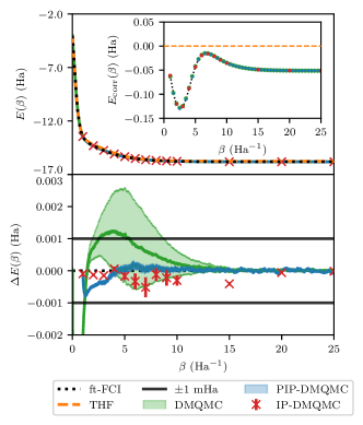
Figure 1: Finite temperature energies for BeH₂ Be/cc-pVDZ H/DZ from a variety of methods. In the top panel, total energies are shown plotted against $\beta$. Energies in the inset are calculated by taking the difference to THF, which is found with Eq. (15). The inset DMQMC and PIP-DMQMC data are re-sampled every 50 points starting from $\beta=1$. In the bottom panel, energy differences with respect to ft-FCI are shown (when $\Delta E$ is positive, ft-FCI is lower in energy). Data here show asymmetric PIP-DMQMC propagation (Eq. (21)). The PIP-DMQMC simulations were initialized with $\beta_{T}=1.0$, allowing data collection at $\beta\geq 1.0$.

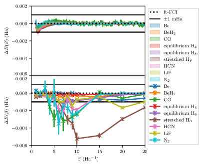
Figure 2: Finite temperature energy differences to ft-FCI are shown for a variety of test systems for PIP-DMQMC (in the top panel) and IP-DMQMC (in the bottom panel). Data here show asymmetric PIP-DMQMC propagation (Eq. (21)). The PIP-DMQMC simulations were initialized with $\beta_{T}=1.0$, allowing data collection at $\beta\geq 1.0$.

Figure 2 compares IP-DMQMC and PIP-DMQMC by looking at all of the test set data. In each case, differences were found between the method and ft-FCI and we are paying particular attention to the mHa error threshhold. Here, we do find that IP-DMQMC has a drift towards lower values at intermediate $\beta$ regimes in most cases which recovers at large $\beta$. A prominent example of this visible in Fig. 2 is stretched H₈, with a maximum deviation at around $\beta=10$. Similar to DMQMC, this appears to be related to how the simulation is initialized; if a particular state is unlikely to be chosen there can be errors due to under-sampling. This would ultimately be remedied if enough $\beta$ loops were run. PIP-DMQMC appears to mostly remedy this, though we note that PIP-DMQMC does tend to have a dip in energy near its crossover point (where it switches propagator). Examples of this are BeH₂ (Fig. 1), and CO in the supporting information.

Overall, therefore, we can conclude that PIP-DMQMC achieves just as good if not better energies than DMQMC and IP-DMQMC across our test set.

For all data presented so far, we have used a $\beta_{T}=1.0$ for PIP-DMQMC. Therefore it is worthwhile checking our conclusions for a range of $\beta_{T}$ values to ensure they are not dependent on $\beta_{T}$. In Fig. 3(a) we plot PIP-DMQMC data for a range of $\beta_{T}$ values from $\beta_{T}=1.0$ to $\beta_{T}=20.0$ using Eq. (21) for the BeH₂ system.

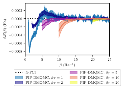
(a)

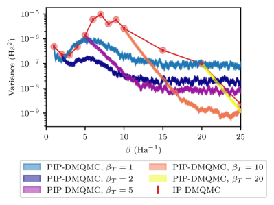
(b)

Figure 3: Energy accuracy and variance of the PIP-DMQMC method using several $\beta_{T}$ values (given in the legends) for BeH₂ Be/cc-pVDZ H/DZ. The impact of changing $\beta_{T}$ for PIP-DMQMC is evaluated using: (a) the energy difference to the ft-FCI energy, and (b) the variance of the energy estimate compared to the IP-DMQMC variance. The $\beta_{T}$ used for IP-DMQMC are the same as the $\beta$ shown in the figure. PIP-DMQMC and IP-DMQMC have the same variance when the two share $\beta_{T}$. For $\beta>\beta_{T}$, the PIP-DMQMC variance is generally below that of IP-DMQMC. The PIP-DMQMC data shown are from asymmetric propagation (Eq. (21)). All data were collected using approximately ten million walkers ($N_{w}=10^{7}$) and averaged over 100 $\beta$ loops ($N_{\beta}=100$).

The accuracy of PIP-DMQMC tended to remain similar or improve across the $\beta_{T}$ used, supporting the prior conclusions made about the method. For the energy difference at $\beta=\beta_{T}$, the accuracy tended to be similar across all the $\beta_{T}$ simulated. For the energy difference at $\beta>\beta_{T}$, the accuracy in general remained similar or shows slight improvement. The one exception being for $\beta_{T}=1.0$ where a notable decrease in accuracy is initially observed. Crucially all lines stay within the target accuracy of $\pm 1$ mHa, which is too large to be shown on the plot range used in Fig. 3(a).

In addition to investigating the accuracy of PIP-DMQMC using several $\beta_{T}$, we investigate the variance of PIP-DMQMC in Fig. 3(b). Both PIP-DMQMC and IP-DMQMC methods have the same variance at $\beta=\beta_{T}$ because we are using the same random number seed. In general the variance peaks at intermediate $\beta$. Comparing the variance from PIP-DMQMC (run beyond the target $\beta$) to the variance from IP-DMQMC, we see, in general, that the PIP-DMQMC variance is similar to or smaller than IP-DMQMC. This is to say that PIP-DMQMC’s use of the Bloch equation tends to decrease variance relative to IP-DMQMC at $\beta>\beta_{T}$. One reason for this could be the way in which IP-DMQMC is initialized. We first recall that the Fermi-Dirac weights are used to select the diagonal matrix elements and that then these are re-weighted for the difference between the Fermi-Dirac density matrix and the Hartree–Fock density matrix (Eq. (17)). The re-weighting happens through spawning a certain number of walkers on this element. When the Fermi-Dirac density matrix is a poor match for the Hartree–Fock density matrix, the re-weighting will be large. However this, in turn, limits the high-energy rows that can be included in the simulation. Over successive $\beta$ loops, our data are consistent with the idea that the variance due to this initialization is larger than propagating from an earlier $\beta$ using the Bloch equation. The consequence of this is that more $\beta$ loops may be required to convergence the stochastic error in IP-DMQMC as compared with PIP-DMQMC.

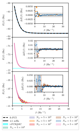
Figure 4: Graphs to show initiator convergence for symmetric i-PIP-DMQMC (Eq. (20)) with increasing walker populations for HBCH₂/STO-3G (top panel), H₂O/cc-pVDZ (middle panel) and CH₄/cc-pVDZ (bottom panel). Not all walker populations were run for all systems. Except for methane, the walker numbers fully overlap on the main graph. To show initiator convergence, the inset shows the energy calculated as a difference to the simulation with the largest walker population for CH₄ and H₂O, and ft-FCI for HBCH₂. The inset only shows the two largest walker populations to make trends more visible. Inset data are re-sampled every 50 points starting from $\beta=1$. The largest walker population was $5\times 10^{8}$ for H₂O and CH₄. $N_{\beta}$ was adjusted between population to give comparable error bars, the details of which are found in the supplementary information. The $N_{w}=5\times 10^{7}$ for HBCH₂ and $N_{w}=5\times 10^{8}$ for H₂O contains one less $\beta$-loop compared to the other systems matching $N_{w}$ data sets. The PIP-DMQMC simulations were initialized with $\beta_{T}=1.0$, allowing data collection at $\beta\geq 1.0$.

Our next test is to find out whether the initiator approximation works well with PIP-DMQMC. The initiator approximation is important for treating larger systems because the critical walker population (also known as a plateau height) rapidly grows beyond what we can store. We found that adding to the initiator space when the site has a population of 3 or greater ($n_{\mathrm{add}}=3$) and having states be initiators if the bra and ket only differ by a double excitation ($n_{\mathrm{ex}}=2$) gives reasonable results; these values were consistent with previous calculations in the uniform electron gas.Malone et al. (2016) As $n_{\mathrm{ex}}$ causes the simulation to have a plateau again, we also must make sure we are above the plateau to overcome the sign problem.

In Fig. 4, we show the results of the initiator adaptation with PIP-DMQMC (i-PIP-DMQMC) on three systems: HBCH₂, H₂O, and CH₄. These calculations were run with a variety of walker numbers so that we could check for initiator convergence, which occurs when the walker number is increased without the energy changing.Cleland, Booth, and Alavi (2010); Booth et al. (2011); Shepherd, Booth, and Alavi (2012) In preliminary calculations, we noted relatively little difference between the two different modes of propagation and decided to use symmetric propagation (Eq. (20)) as this had been shown to reduce stochastic noise in previous studies.Malone (2017)

In general, we see that the plots for different systems at different walker numbers generally overlay one another. The exception to this is low walker populations for CH₄, and this is an example where the population is below the effective $n_{\mathrm{ex}}=2$ plateau height at intermediate $\beta$. Each plot includes an inset where the difference is taken to the largest walker population for H₂O and CH₄ and to ft-FCI for HBCH₂. For HBCH₂, we show the convergence to ft-FCI in the inset. At the highest walker population, the systematic error generally falls to $\sim 1$mHa for most $\beta$ values. At its peak, the systematic error reaches $\sim 2$mHa at $\beta$ at the highest population. For H₂O and CH₄, where we do not have ft-FCI results available, the inset instead shows the energy difference to the largest walker number (which is taken to be the best estimate we have). We find that, for high $\beta$, the initiator error is well converged. Between $N_{w}=5\times 10^{7}$ and $N_{w}=5\times 10^{8}$, the energy difference is submillihartree above $\beta>5$ and $\beta>10$ for H₂O and CH₄ respectively. For the smaller $\beta$ values for both systems, the stochastic error rises sharply to an order of magnitude higher (i.e. $\sim 0.01$Ha). Any systematic initiator error is difficult to estimate due to this increase in stochastic error. In general, this shows significant promise for PIP-DMQMC and highlights the advantage of having so much data over the $\beta$ range available.

One final consideration is that of computational cost. The cost ($C$) of a simulation can be considered to be proportionate to the total amount of $\beta$ that is simulated. In IP-DMQMC, sampling from an initial inverse temperature 0 to a final inverse temperature $\beta$ with even spacing ($\Delta\beta$) results in a cost: $C\propto\beta\left(\frac{\beta}{2\Delta\beta}+\frac{1}{2}\right)$. By contrast, PIP-DMQMC has a scaling of: $C\propto\beta$, which is the same as IP-DMQMC when $\Delta\beta=1$ and a temperature range is not being sampled. IP-DMQMC increases in cost as more $\beta$ values are sampled and has an asymptotic scaling of $\mathcal{O}(\beta^{2})$, while PIP-DMQMC costs $\mathcal{O}(\beta)$. In this way, PIP-DMQMC can be seen to both have an improved cost and resolution of the energy as a function of $\beta$.

VI Conclusions

In summary, we have introduced a piecewise generalization of the interaction picture propagator in density matrix quantum Monte Carlo, which leads to us being able to sample a wide range of temperatures with a single calculation. In proof of concept calculations on a variety of molecular systems, PIP-DMQMC is generally at least as accurate as IP-DMQMC and DMQMC. The result is a reduction in calculation cost to sample energies at 0 to $\beta$ from $\mathcal{O}(\beta^{2})$ to $\mathcal{O}(\beta)$ while also obtaining more data points. Furthermore, we see an improvement of sampling statistics especially at large $\beta$ and have the ability to see more convergence data for the initiator approximation. We hope that others can use the water and methane calculations for benchmarking their calculations.

Taken together, our results show that PIP-DMQMC is a promising development for DMQMC. Our long-term goal is to make DMQMC a resource for benchmarking finite temperature methods development He, Ryu, and Hirata (2014); Santra and Schirmer (2017); Hirata and Jha (2020); Jha and Hirata (2020); Hirata (2021); Dzhioev and Kosov (2015); Hermes and Hirata (2015); Hummel (2018); Harsha, Henderson, and Scuseria (2019); White and Chan (2019); Shushkov and Miller (2019); White and Kin-Lic Chan (2020); Peng et al. (2021); Harsha et al. (2022) as well as describing electronic structure phenomena at finite temperature. With this in mind, two limitations of our study were that we did not systematically study convergence with initiator parameters or with starting initialization. These are interrelated because they both cause systematic biases in the energy and so efforts have to be made to separate out and measure the two effects. We are in the process of preparing a forthcoming manuscript on this topic.Van Benschoten and Shepherd

VII Acknowledgements

Research was supported by the U.S. Department of Energy, Office of Science, Office of Basic Energy Sciences Early Career Research Program (ECRP) under Award Number DE-SC0021317.

This research also used resources from the University of Iowa and the resources of the National Energy Research Scientific Computing Center, a DOE Office of Science User Facility supported by the Office of Science of the U.S. Department of Energy under Contract No. DE-AC02-05CH11231 (computer time for calculations only).

This research used a locally modified version of the development branch of HANDE-QMC.Spencer et al. (2019) The code will be queued for public release after the manuscript is published. For the purposes of providing information about the calculations used, files will be deposited with Iowa Research Online (IRO) with a reference number [to be inserted at production].

VIII Data Availability

The data that supports the findings of this study are available within the article.

References

- Militzer et al. (2016) B. Militzer, F. Soubiran, S. M. Wahl, and W. Hubbard, Journal of Geophysical Research: Planets 121, 1552 (2016).
- Mazzola, Helled, and Sorella (2018) G. Mazzola, R. Helled, and S. Sorella, Physical Review Letters 120, 025701 (2018).
- Mukherjee et al. (2013) S. Mukherjee, F. Libisch, N. Large, O. Neumann, L. V. Brown, J. Cheng, J. B. Lassiter, E. A. Carter, P. Nordlander, and N. J. Halas, Nano Letters 13, 240 (2013).
- Zhou et al. (2016) L. Zhou, C. Zhang, M. J. McClain, A. Manjavacas, C. M. Krauter, S. Tian, F. Berg, H. O. Everitt, E. A. Carter, P. Nordlander, and N. J. Halas, Nano Letters 16, 1478 (2016).
- Ernstorfer et al. (2009) R. Ernstorfer, M. Harb, C. T. Hebeisen, G. Sciaini, T. Dartigalongue, and R. J. D. Miller, Science 323, 1033 (2009).
- Gull, Parcollet, and Millis (2013) E. Gull, O. Parcollet, and A. J. Millis, Physical Review Letters 110, 216405 (2013).
- Drummond et al. (2015) N. D. Drummond, B. Monserrat, J. H. Lloyd-Williams, P. L. Ríos, C. J. Pickard, and R. J. Needs, Nature Communications 6, 7794 (2015).
- He, Ryu, and Hirata (2014) X. He, S. Ryu, and S. Hirata, The Journal of Chemical Physics 140, 024702 (2014).
- Santra and Schirmer (2017) R. Santra and J. Schirmer, Chemical Physics 482, 355 (2017).
- Hirata and Jha (2020) S. Hirata and P. K. Jha, The Journal of Chemical Physics 153, 014103 (2020).
- Jha and Hirata (2020) P. K. Jha and S. Hirata, Physical Review E 101, 022106 (2020).
- Hirata (2021) S. Hirata, The Journal of Chemical Physics 155, 094106 (2021).
- Dzhioev and Kosov (2015) A. A. Dzhioev and D. S. Kosov, Journal of Physics A: Mathematical and Theoretical 48, 015004 (2015).
- Hermes and Hirata (2015) M. R. Hermes and S. Hirata, The Journal of Chemical Physics 143, 102818 (2015).
- Hummel (2018) F. Hummel, Journal of Chemical Theory and Computation 14, 6505 (2018).
- Harsha, Henderson, and Scuseria (2019) G. Harsha, T. M. Henderson, and G. E. Scuseria, The Journal of Chemical Physics 150, 154109 (2019).
- White and Chan (2019) A. F. White and G. K.-L. Chan, Journal of Chemical Theory and Computation 15, 6137 (2019).
- Shushkov and Miller (2019) P. Shushkov and T. F. Miller, The Journal of Chemical Physics 151, 134107 (2019).
- White and Kin-Lic Chan (2020) A. F. White and G. Kin-Lic Chan, The Journal of Chemical Physics 152, 224104 (2020).
- Peng et al. (2021) R. Peng, A. F. White, H. Zhai, and G. Kin-Lic Chan, The Journal of Chemical Physics 155, 044103 (2021).
- Harsha et al. (2022) G. Harsha, Y. Xu, T. M. Henderson, and G. E. Scuseria, Physical Review B 105, 045125 (2022).
- Karasiev, Sjostrom, and Trickey (2012) V. V. Karasiev, T. Sjostrom, and S. B. Trickey, Physical Review B 86, 115101 (2012).
- Ellis et al. (2021) J. A. Ellis, L. Fiedler, G. A. Popoola, N. A. Modine, J. A. Stephens, A. P. Thompson, A. Cangi, and S. Rajamanickam, Physical Review B 104, 035120 (2021).
- Pittalis et al. (2011) S. Pittalis, C. R. Proetto, A. Floris, A. Sanna, C. Bersier, K. Burke, and E. K. U. Gross, Physical Review Letters 107, 163001 (2011).
- Eschrig (2010) H. Eschrig, Physical Review B 82, 205120 (2010).
- Pribram-Jones, Grabowski, and Burke (2016) A. Pribram-Jones, P. E. Grabowski, and K. Burke, Physical Review Letters 116, 233001 (2016).
- Kananenka et al. (2016) A. A. Kananenka, A. R. Welden, T. N. Lan, E. Gull, and D. Zgid, Journal of Chemical Theory and Computation 12, 2250 (2016).
- Welden, Rusakov, and Zgid (2016) A. R. Welden, A. A. Rusakov, and D. Zgid, The Journal of Chemical Physics 145, 204106 (2016).
- Kas and Rehr (2017) J. Kas and J. Rehr, Physical Review Letters 119, 176403 (2017).
- Karrasch, Meden, and Schönhammer (2010) C. Karrasch, V. Meden, and K. Schönhammer, Physical Review B 82, 125114 (2010).
- Neuhauser, Baer, and Zgid (2017) D. Neuhauser, R. Baer, and D. Zgid, Journal of Chemical Theory and Computation 13, 5396 (2017).
- Gu et al. (2020) J. Gu, J. Chen, Y. Wang, and X.-G. Zhang, Computer Physics Communications 253, 107178 (2020).
- Li et al. (2020) J. Li, M. Wallerberger, N. Chikano, C.-N. Yeh, E. Gull, and H. Shinaoka, Physical Review B 101, 035144 (2020).
- Knizia and Chan (2013) G. Knizia and G. K.-L. Chan, Journal of Chemical Theory and Computation 9, 1428 (2013).
- Sun et al. (2020) C. Sun, U. Ray, Z.-H. Cui, M. Stoudenmire, M. Ferrero, and G. K.-L. Chan, Physical Review B 101, 075131 (2020).
- Kretchmer and Chan (2018) J. S. Kretchmer and G. K.-L. Chan, The Journal of Chemical Physics 148, 054108 (2018).
- Tran, Van Voorhis, and Thom (2019) H. K. Tran, T. Van Voorhis, and A. J. W. Thom, The Journal of Chemical Physics 151, 034112 (2019).
- Cui, Zhu, and Chan (2020) Z.-H. Cui, T. Zhu, and G. K.-L. Chan, Journal of Chemical Theory and Computation 16, 119 (2020).
- Zhai and Chan (2021) H. Zhai and G. K.-L. Chan, The Journal of Chemical Physics 154, 224116 (2021).
- Tsuchimochi, Welborn, and Van Voorhis (2015) T. Tsuchimochi, M. Welborn, and T. Van Voorhis, The Journal of Chemical Physics 143, 024107 (2015).
- Bulik, Chen, and Scuseria (2014) I. W. Bulik, W. Chen, and G. E. Scuseria, The Journal of Chemical Physics 141, 054113 (2014).
- Hermes and Gagliardi (2019) M. R. Hermes and L. Gagliardi, Journal of Chemical Theory and Computation 15, 972 (2019).
- Zgid and Gull (2017) D. Zgid and E. Gull, New Journal of Physics 19, 023047 (2017).
- Lan and Zgid (2017) T. N. Lan and D. Zgid, The Journal of Physical Chemistry Letters 8, 2200 (2017).
- Tran, Iskakov, and Zgid (2018) L. N. Tran, S. Iskakov, and D. Zgid, The Journal of Physical Chemistry Letters 9, 4444 (2018).
- Rusakov et al. (2019) A. A. Rusakov, S. Iskakov, L. N. Tran, and D. Zgid, Journal of Chemical Theory and Computation 15, 229 (2019).
- Dornheim et al. (2015) T. Dornheim, S. Groth, A. Filinov, and M. Bonitz, New Journal of Physics 17, 073017 (2015).
- Militzer and Driver (2015) B. Militzer and K. P. Driver, Physical Review Letters 115, 176403 (2015).
- Larkin and Filinov (2017) A. S. Larkin and V. S. Filinov, Journal of Applied Mathematics and Physics 05, 392 (2017).
- Groth, Dornheim, and Bonitz (2017) S. Groth, T. Dornheim, and M. Bonitz, The Journal of Chemical Physics 147, 164108 (2017).
- Dornheim et al. (2018) T. Dornheim, S. Groth, J. Vorberger, and M. Bonitz, Physical Review Letters 121, 255001 (2018).
- Dornheim (2019) T. Dornheim, Physical Review E 100, 023307 (2019).
- Yilmaz et al. (2020) A. Yilmaz, K. Hunger, T. Dornheim, S. Groth, and M. Bonitz, The Journal of Chemical Physics 153, 124114 (2020).
- Dornheim et al. (2021) T. Dornheim, M. Böhme, B. Militzer, and J. Vorberger, Physical Review B 103, 205142 (2021).
- Lee, Chen, and Kao (2012) C.-R. Lee, Z.-H. Chen, and Q.-L. Kao, in 2012 IEEE 26th International Parallel and Distributed Processing Symposium Workshops & PhD Forum (IEEE, Shanghai, China, 2012) pp. 1889–1897.
- Chang et al. (2015) C.-C. Chang, S. Gogolenko, J. Perez, Z. Bai, and R. T. Scalettar, Philosophical Magazine 95, 1260 (2015).
- Liu, Cho, and Rubenstein (2018) Y. Liu, M. Cho, and B. Rubenstein, Journal of Chemical Theory and Computation 14, 4722 (2018).
- He et al. (2019) Y.-Y. He, M. Qin, H. Shi, Z.-Y. Lu, and S. Zhang, Physical Review B 99, 045108 (2019).
- Shen et al. (2020) T. Shen, Y. Liu, Y. Yu, and B. M. Rubenstein, The Journal of Chemical Physics 153, 204108 (2020).
- Church and Rubenstein (2021) M. S. Church and B. M. Rubenstein, The Journal of Chemical Physics 154, 184103 (2021).
- Liu et al. (2020) Y. Liu, T. Shen, H. Zhang, and B. Rubenstein, Journal of Chemical Theory and Computation 16, 4298 (2020).
- Blunt, Alavi, and Booth (2015) N. Blunt, A. Alavi, and G. H. Booth, Physical Review Letters 115, 050603 (2015).
- Blunt et al. (2014) N. S. Blunt, T. W. Rogers, J. S. Spencer, and W. M. C. Foulkes, Physical Review B 89, 245124 (2014).
- Booth, Thom, and Alavi (2009) G. H. Booth, A. J. W. Thom, and A. Alavi, The Journal of Chemical Physics 131, 054106 (2009).
- Malone et al. (2015) F. D. Malone, N. S. Blunt, J. J. Shepherd, D. K. K. Lee, J. S. Spencer, and W. M. C. Foulkes, The Journal of Chemical Physics 143, 044116 (2015).
- Cleland, Booth, and Alavi (2010) D. Cleland, G. H. Booth, and A. Alavi, The Journal of Chemical Physics 132, 041103 (2010).
- Dornheim et al. (2017) T. Dornheim, S. Groth, F. D. Malone, T. Schoof, T. Sjostrom, W. M. C. Foulkes, and M. Bonitz, Physics of Plasmas 24, 056303 (2017).
- Groth et al. (2017) S. Groth, T. Dornheim, T. Sjostrom, F. D. Malone, W. Foulkes, and M. Bonitz, Physical Review Letters 119, 135001 (2017).
- Dornheim et al. (2016) T. Dornheim, S. Groth, T. Sjostrom, F. D. Malone, W. Foulkes, and M. Bonitz, Physical Review Letters 117, 156403 (2016).
- Petras et al. (2020) H. R. Petras, S. K. Ramadugu, F. D. Malone, and J. J. Shepherd, Journal of Chemical Theory and Computation 16, 1029 (2020).
- Petras et al. (2021) H. R. Petras, W. Z. Van Benschoten, S. K. Ramadugu, and J. J. Shepherd, Journal of Chemical Theory and Computation 17, 6036 (2021).
- Chessex, Borrelli, and Öttinger (2022) R. Chessex, M. Borrelli, and H. C. Öttinger, (2022), 10.48550/ARXIV.2201.01383, publisher: arXiv Version Number: 1.
- Kou and Hirata (2014) Z. Kou and S. Hirata, Theoretical Chemistry Accounts 133, 1487 (2014).
- Malone et al. (2016) F. D. Malone, N. Blunt, E. W. Brown, D. Lee, J. Spencer, W. Foulkes, and J. J. Shepherd, Physical Review Letters 117, 115701 (2016).
- Cleland, Booth, and Alavi (2011) D. M. Cleland, G. H. Booth, and A. Alavi, The Journal of Chemical Physics 134, 024112 (2011).
- Cleland et al. (2012) D. Cleland, G. H. Booth, C. Overy, and A. Alavi, Journal of Chemical Theory and Computation 8, 4138 (2012).
- Shepherd, Booth, and Alavi (2012) J. J. Shepherd, G. H. Booth, and A. Alavi, The Journal of Chemical Physics 136, 244101 (2012).
- Booth et al. (2013) G. H. Booth, A. Grüneis, G. Kresse, and A. Alavi, Nature 493, 365 (2013).
- Thomas, Booth, and Alavi (2015) R. E. Thomas, G. H. Booth, and A. Alavi, Physical Review Letters 114, 033001 (2015).
- (80) In the grand canonical initialization scheme introduced at the same time as IP-DMQMCMalone et al. (2015), the walker number was interpreted as the number of times initialization was attempted. For this paper, this was modified to instead count the number of walkers created.
- Malone (2017) F. D. Malone, Quantum Monte Carlo Simulations of Warm Dense Matter, Ph.D. thesis (2017).
- Spencer et al. (2019) J. S. Spencer, N. S. Blunt, S. Choi, J. Etrych, M.-A. Filip, W. M. C. Foulkes, R. S. T. Franklin, W. J. Handley, F. D. Malone, V. A. Neufeld, R. Di Remigio, T. W. Rogers, C. J. C. Scott, J. J. Shepherd, W. A. Vigor, J. Weston, R. Xu, and A. J. W. Thom, Journal of Chemical Theory and Computation 15, 1728 (2019).
- Bernath et al. (2002) P. F. Bernath, A. Shayesteh, K. Tereszchuk, and R. Colin, Science 297, 1323 (2002).
- Herzberg (1966) G. Herzberg, Electronic spectra and electronic structure of polyatomic molecules, Vol. 3 (van Nostrand, 1966).
- Frisch et al. (2009) M. Frisch, G. Trucks, H. B. Schlegel, G. E. Scuseria, M. A. Robb, J. R. Cheeseman, G. Scalmani, V. Barone, B. Mennucci, G. Petersson, and others, Inc., Wallingford CT 201 (2009).
- Lovas (2002) F. Lovas, “Diatomic Spectral Database, NIST Standard Reference Database 114,” (2002), type: dataset.
- Wharton et al. (1963) L. Wharton, W. Klemperer, L. P. Gold, R. Strauch, J. J. Gallagher, and V. E. Derr, The Journal of Chemical Physics 38, 1203 (1963).
- Johnson and others (2006) R. D. Johnson and others, http://srdata.nist.gov/cccbdb (2006).
- Werner et al. (2019) H.-J. Werner, P. J. Knowles, G. Knizia, F. R. Manby, M. Schütz, and others, “MOLPRO, 2019.2 , a package of ab initio programs,” (2019), see https://www.molpro.net.
- Booth et al. (2011) G. H. Booth, D. Cleland, A. J. W. Thom, and A. Alavi, The Journal of Chemical Physics 135, 084104 (2011).
- (91) W. Z. Van Benschoten and J. J. Shepherd, Unpublished.