Is there any linkage between interstellar aldehyde and alcohol?

Abstract

It is speculated that there might be some linkage between interstellar aldehydes and their corresponding alcohols. Here, an observational study and astrochemical modeling are coupled together to illustrate the connection between them. The ALMA cycle 4 data of a hot molecular core, G10.47+0.03 is utilized for this study. Various aldehydes (acetaldehyde, propanal, and glycolaldehyde), alcohols (methanol and ethylene glycol), and a ketone (acetone) are identified in this source. The excitation temperatures and the column densities of these species were derived via the rotation diagram method assuming LTE conditions. An extensive investigation is carried out to understand the formation of these species. Six pairs of aldehyde-alcohol: i) methanal and methanol; ii) ethanal and ethanol; iii) propanal and 1-propanol; iv) propenal and allyl alcohol; v) propynal and propargyl alcohol; vi) glycolaldehyde and ethylene glycol; vii) along with one pair of ketone-alcohol (acetone and isopropanol) and viii) ketene-alcohol (ethenone and vinyl alcohol) are considered for this study. Two successive hydrogenation reactions in the ice phase are examined to form these alcohols from aldehydes, ketone, and ketene, respectively. Quantum chemical methods are extensively executed to review the ice phase formation route and the kinetics of these species. Based on the obtained kinetic data, astrochemical modeling is employed to derive the abundances of these aldehydes, alcohols, ketone, and ketene in this source. It is seen that our model could successfully explain the observed abundances of various species in this hot molecular core.

1 Introduction

More than 200 molecular species have been identified in the interstellar medium (ISM) and circumstellar shells (McGuire, 2018, https://cdms.astro.uni-koeln.de/classic/molecules), which resolved the much-unexplained mystery of the molecular Universe. Interstellar grains accelerate the formation of Complex Organic Molecules (COMs, molecule with $>$ 6 atoms) in space. During the warm-up phase of a star-forming core, radicals or simple molecules on the grain surface become mobile and could produce various COMs (Chakrabarti et al., 2006a, b; Garrod & Herbst, 2006; Garrod et al., 2008; Das et al., 2008a, 2010; Das & Chakrabarti, 2011; Das et al., 2016; Sil et al., 2018). These ice phase species may transfer to the gas phase by various desorption mechanisms.

Alcohols and aldehydes were identified in various parts of the ISM. Methanal (formaldehyde, $\rm{H_{2}CO}$) is the simplest form of aldehydes, which was first observed in space by Snyder et al. (1969). It is an intermediary of the large complex organic molecules, which can help constrain physical conditions in the star-forming regions (Persson et al., 2018). Methanol (methyl alcohol, $\rm{CH_{3}OH}$) is the simplest alcohol and is one of the most abundant interstellar molecules. It was widely observed toward various sources (Allamandola et al., 1992; Pontoppidan et al., 2003) and is used as a reliable tracer of high-density environments (Menten et al., 1988). A wide number of studies reported the chemical origin of methanol starting from formaldehyde (Watanabe & Kouchi, 2002; Fuchs et al., 2009; Goumans, 2011; Song & Kästner, 2017). Methanol is ubiquitous in star-forming regions (Weaver et al., 2018) and is mainly formed on the interstellar dust via successive hydrogen addition reactions with carbon monoxide (Fedoseev et al., 2015; Chuang et al., 2016; Butscher et al., 2017).

Woon (2002a) carried out a theoretical study of the formation of H₂CO and CH₃OH. Quantum chemical calculations were carried out to determine the activation barrier for the hydrogen addition reactions ($\rm{H+CO}$ and $\rm{H+H_{2}CO}$) in gas, with water clusters $\rm(H_{2}O)_{n}$ (n$\leq 3$) and in ice phases. He included explicit water molecules to show the catalytic effect on the activation barrier by surrounding water molecules. Rimola et al. (2014); Das et al. (2008b) studied methanol formation by successive hydrogen addition with CO in water ice. They compared their simulated abundance with observations. Recently, Song & Kästner (2017) derived the tunneling rate constant of H₂CO + H reaction on amorphous solid water for various product channels: CH₂OH, CH₃O, and H₂ + HCO. They also provided the activation barrier of these three product channels and rate coefficients.

Identification of ethanal (CH₃CHO, acetaldehyde) was first reported by Gottlieb (1973) toward Sgr B2 and Sgr A. They reported an emission at $1065$ MHz, which was assigned to the $1_{10}\rightarrow 1_{11}$ transition of CH₃CHO. This assignment was based on the agreement in radial velocity with other molecules, which were observed in the galactic center region. Then Fourikis et al. (1974) observed it toward Sgr B2 with the Parkes 64m telescope. Its successor, ethanol ($\rm{C_{2}H_{5}OH}$, ethyl alcohol), is among the earliest complex molecules, which was identified toward the Sgr B2 (Zuckerman et al., 1975).

Propanal ($\rm{CH_{3}CH_{2}CHO}$, propionaldehyde) is identified in Sgr B2(N) (Hollis et al., 2004), where it coexists with propynal (HC₂CHO) and propenal (CH₂CHCHO). The detection of these three aldehydes toward the same source suggests that successive hydrogen additions might be an efficient process to establish the chemical linkage between propynal, propenal, and propanal (Hollis et al., 2004). Propenal (also known as acrolein) is the simplest unsaturated aldehyde. It is the second most stable isomer of the $\rm{C_{3}H_{4}O}$ isomeric group (Etim et al., 2018). Allyl alcohol (CH₂CHCH₂OH) is an isomer of propanal and the corresponding alcohol of propenal (Zaverkin et al., 2018). Acetaldehyde is supposed to be a potential ancestor of carbohydrates and propenal (also known as acrolein) (Pizzarello & Weber, 2004; Córdova et al., 2005).

The corresponding alcohol of propanal is 1-propanol ($\rm{CH_{3}CH_{2}CH_{2}OH}$), which is yet to be observed in space. However, trans-ethyl methyl ether ($\rm{CH_{3}CH_{2}OCH_{3}}$), which is one of the isomers of the same isomeric group, was tentatively detected toward Orion KL (Tercero et al., 2015). Zaverkin et al. (2018) reported that the propanal to 1-propanol production by the hydrogenation reaction might be inefficient due to the efficient hydrogen abstraction reaction.

The simplest form of sugar, glycolaldehyde (HOCH₂CHO), plays an essential role in forming amino acids and complex sugars (Weber, 1998; Collins et al., 1995). Glycolaldehyde was also detected outside of the Galactic Center towards the hot core G31.41+0.31 (Beltrán et al., 2009) (hereafter, G31). Ethylene glycol (HOCH₂CH₂OH) is the corresponding alcohol of glycolaldehyde. It was detected in a wide variety of sources such as in the Galactic Center (Hollis et al., 2002; Belloche et al., 2013), NGC 1333-IRAS 2A (Maury et al., 2014), Orion bar (Brouillet et al., 2015) and also in the comets C/1995 O1 (Hale-Bopp) (Crovisier et al., 2004), C/2012 F6 (Lemmon) and C/2013 R1 (Lovejoy) (Biver et al., 2014). It was also identified in the Murchinson and Murray meteorites (Cooper et al., 2001). The abundance ratio of glycolaldehyde and ethylene glycol in star-forming regions and comets can help understand the possible preservation of complex organic molecules (Coutens et al., 2018). Methyl formate (CH₃OCHO) and acetic acid (CH₃COOH) are two isomers of glycolaldehyde. The linkage between the methyl formate, acetic acid, and glycolaldehyde can constrain the understanding of the chemical and physical conditions of the star-forming core (Woods et al., 2013). Acetone ($\rm{CH_{3}COCH_{3}}$) is one of the most important molecules in organic chemistry, and it was the first species containing $10$ atoms identified in the ISM (Combes et al., 1987). Acetone was also found to be present in the comet 67P/Churyumov-Gerasimenko (Altwegg et al., 2017). Ethenone (CH₂CO, ketene) was identified for the first time toward Sgr B2(OH) by Turner (1977) through microwave measurements. Recently, Turner et al. (2020) perform experiment combined with high-level quantum chemical calculations and provide compelling evidence of ketene formation in the processed mixture of water and carbon monoxide ices explaining the observed ketene detection in deep space. The simplest enol compound, vinyl alcohol (CH₂CHOH, ethenol), was identified in an interstellar cloud of dust and gas near the center of the Milky Way galaxy toward Sgr B2(N) utilizing its millimeter-wave rotational transitions (Turner & Apponi, 2001). In the dark cloud, the non-energetic process plays an active role in processing the ice constituents. In contrast, in the latter stages of star and planet formation, various energetic procedures play a crucial role (Fedoseev et al., 2017). Laboratory experiments of methanol dissociation studied through various energetic processes, such as photons, electrons, Vacuum Ultraviolet (VUV) photons, X-ray, etc. that could lead to the synthesis of various COMs. Öberg et al. (2009) found that the ratio between ethylene glycol to ethanol and methyl formate to ethanol varies with the ice temperature and irradiation.

In this work, ALMA archival data of a hot molecular core, G10.47+0.03 is analyzed which is located at a distance of 8.6 kpc (Sanna et al., 2014). This is a young cluster (Cesaroni et al., 1998; Rolffs et al., 2011) whose luminosity is $\sim\rm{5\times 10^{5}\ L_{\odot}}$ Cesaroni et al. (2010). Many simple species, complex organics, and molecules with higher upper energy state (such as HC₃N, HCN) were observed in this source, suggesting an active site for the chemical enrichment (Ikeda et al., 2001; Wyrowski et al., 1999; Gibb et al., 2004; Rolffs et al., 2011; Gorai et al., 2020).

Recently Qasim et al. (2019) showed that the aldehyde and primary alcohol may be linked via successive hydrogen addition reactions. A similar connection is also observed between ketones and secondary alcohols, i.e., isopropanol ($\rm{CH_{3}CHOHCH_{3}}$) can be synthesized via two successive hydrogen additions with acetone (Hiraoka et al., 1998). Here, several aldehydes and alcohols are identified. Obtained column density, rotation temperature, spatial distributions of these molecules are discussed to understand the morphological correlation between these aldehydes and alcohols. The astrochemical model is implemented to compare with the observational finding. This work demonstrates that consecutive hydrogen addition could contribute to forming some complex interstellar molecules. Here, the kinetics of the consecutive hydrogen addition reactions of alcohol production from aldehyde, ketone, and ketene are examined. Binding energies (BEs) of a species with a grain substrate are essential for constructing a chemical model. Most COMs are primarily produced on the dust surface and further desorbed back to the gas phase (Requena-Torres et al., 2006). Most of the time, BE of these species is estimated, which may induce uncertainties in the results. Our estimated BE values with the water ice surface are included in our chemical model to see their impact. The proton affinity (PA) is not directly included in our model. But it is computed to check the reactivity of these species with H⁺. The role of PA of various species and their intermediate steps is also discussed to synthesize new COMs. Some of our obtained kinetic parameters are directly included in our chemical model to compare between the observation and modeling yields.

The remainder of this paper is organized as follows. In Section 2, the observational results are presented. The computational details adopted to explain the chemical linkage between aldehyde and alcohol are given in Section 3. Astrochemical modeling and its implication are discussed in Section 4 and finally in Section 5, we conclude.

2 Observations of a hot molecular core, G10.47+0.03

2.1 Observations and data analysis

This paper uses the ALMA cycle 4 archival data (12m array data) of the observations ($\#$2016.1.00929.S) of G10.47+0.03 (hereafter, G10). The pointing center of the G10 observations is located at $\alpha$(J2000) = 18^h08^m38$\fs$232, $\delta$ (J2000) =-19^∘51$\arcmin$50$\farcs$4. This observation was performed with band 4 having four spectral bands covering the sky frequencies of $129.50-131.44$ GHz, $147.50-149.43$ GHz, $153.00-154.93$ GHz, and $158.49-160.43$ GHz and corresponding angular resolution at four different frequencies are $1.67^{{}^{\prime\prime}}$ (14362 AU), $1.52^{{}^{\prime\prime}}$ (13072 AU), $1.66^{{}^{\prime\prime}}$ (14276 AU), and $1.76^{{}^{\prime\prime}}$ (15136 AU) respectively. The spectral resolution of the data is 976 kHz. The number of antennas used for the corresponding four spectral windows are 39, 40, 41 and 39, respectively. The flux calibrator, phase calibrator, and bandpass calibrator of this observation were J1733-1304, J1832-2039, and J1924-2914. The systemic velocity of the source is $68$ km s^-1 (Rolffs et al., 2011). A detailed description of the observations was presented in Gorai et al. (2020). Here, all the analysis (spectral and line analysis) are carried out by using CASA 4.7.2 software (McMullin et al., 2007). Since G10 is a line-rich source, the corrected sigma-clipping method of the STATCONT package (Sánchez-Monge et al., 2018) are used to determine the continuum level in data cube. Further, the spectral window of the data cube is divided into two data cubes (continuum and line emission), using the ‘uvcontsub’ command in the CASA program. Line identification is performed with the CASSIS (Vastel et al., 2015) (This software has been developed by IRAP-UPS/CNRS (http://cassis.irap.omp.eu), which uses the Cologne Database for Molecular Spectroscopy (CDMS, Müller et al., 2001, 2005; Endres et al., 2016) and Jet Propulsion Laboratory (JPL, Pickett et al., 1998) databases. Various physical parameters ($\rm V_{LSR}$, line blending, upper-state energy, Einstein coefficient, and 3 sigma significance level) are considered. LTE synthetic spectra are generated with the best-fitted parameters to compare the observed spectral feature and line identification. We have also used the https://splatalogue.online for the additional confirmation of our choices.

Table 1: Summary of the line parameters of the observed molecules toward G10.47+0.03.

Species	${\rm J^{{}^{\prime}}_{K_{a}^{{}^{\prime}}K_{c}^{{}^{\prime}}}}$-${\rm J^{{}^{\prime\prime}}_{K_{a}^{{}^{\prime\prime}}K_{c}^{{}^{\prime\prime}}}}$	Frequency	Eu	$\Delta$V	Imax	VLSR	S$\mu^{2}$	$\int{T_{mb}}dV$
		(GHz)	(K)	(km s-1)	(K)	(km s-1)	(Debye2)	(K km s-1)
Methanol	$\rm{21_{-0,21}-21_{1,21}}$E, vt=0	129.720384	546.2	9.6$\pm$0.2	30.1$\pm$0.6	66.9$\pm$0.1	19.8	308.7$\pm$14.5
($\rm{CH_{3}OH}$)	$\rm{17_{-4,13}-18_{-3,16}}$E, vt=0	131.134094	450.9	11.1$\pm$0.2	45.7$\pm$0.5	66.6$\pm$0.5	21.8	540.0$\pm$17.7
	$\rm{7_{-1,7}-6_{0,6}}$E, vt=1	147.943673	356.3	11.1$\pm$0.8	32.1$\pm$1.9	66.2$\pm$0.4	14.4	378.5$\pm$52.8
	$\rm{15_{-0,15}-15_{1,15}}$E, vt=0	148.111993	290.7	10.5$\pm$0.6	44.7$\pm$1.5	66.5$\pm$0.2	29.02	500.0$\pm$47.2
	$\rm{8_{-7,1}-7_{-6,1}}$E, vt=1	153.128697	664.5	10.4$\pm$0.2	9.15$\pm$0.1	66.8$\pm$0.1	15.9	101.1$\pm$3.1
	$\rm{12_{-0,12}-15_{1,12}}$E, vt=0	153.281282∗	193.8	11.37$\pm$0.2	40.28$\pm$0.6	66.3$\pm$0.1	30.7	487.4$\pm$14.5
	$\rm{11_{-0,11}-11_{1,11}}$ E, vt=0	154.425832∗	166.1	10.6$\pm$0.3	36.02$\pm$0.7	66.64$\pm$0.1	30.5	408.0$\pm$18.7
Ethylene Glycol	$\rm{33_{10,23}-32_{11,22}}$, 1-1	130.115657	323	7.7$\pm$0.07	2.55$\pm$0.01	67.8$\pm$ 0.03	53	20.9$\pm$0.3
(CH2OH)2	$\rm{13_{9,4}-12_{9,3}}$, 0-1	130.998583	83.7	7.9$\pm$0.5	5.6$\pm$0.24	68.2$\pm$0.178	98.4	48.1$\pm$5.02
	$\rm{28_{7,21}-28_{6,23}}$, 1-0	131.229156	223.4	7.8$\pm$0.1	4.8$\pm$0.02	68.8$\pm$ 0.04	158.3	39.8$\pm$0.7
	$\rm{27_{3,25}-27_{2,26}}$, 0-0	148.082465	185.5	7.2$\pm$0.13	4.8$\pm$0.15	69.3$\pm$0.12	87.3	36.89$\pm$1.8
	$\rm{39_{8,32}-39_{7,33}}$, 1-1	153.325448	414	10.5$\pm$0.5	3.9$\pm$0.1	69.4$\pm$0.15	385.1	44.14$\pm$3.13
	$\rm{8_{4,5}-7_{3,5}}$, 1-0	153.567383	25.4	8.9$\pm$0.27	13.8$\pm$0.33	66.9$\pm$0.11	60.4	131.45$\pm$7.08
	$\rm{13_{3,11}-12_{2,10}}$, 0-0	159.768239	48.8	8.73$\pm$0.25	9.32$\pm$0.15	68.4$\pm$0.08	62.8	86.65$\pm$3.87
Acetaldehyde	$\rm{8_{5,4}-7_{5,3}}$,A	154.161467	89.8	7.3$\pm$0.7	5.0$\pm$0.4	67.6$\pm$0.3	61.7	38.8$\pm$0.10
($\rm{CH_{3}CHO}$)	$\rm{8_{3,5}-7_{3,4}}$,A	154.173895	114.4	6.6$\pm$0.2	1.3$\pm$0.1	67.8$\pm$0.1	44.3	9.2$\pm$0.53
	$\rm{8_{4,4}-7_{4,3}}$,A	154.201471	69.5	8.8$\pm$0.5	5.7$\pm$0.2	67.0$\pm$0.2	75.9	52.9$\pm$0.08
	$\rm{8_{3,6}-7_{3,5}}$,A	154.274686	53.7	8.4$\pm$0.2	5.3$\pm$0.1	67.1$\pm$0.7	87.0	47.5$\pm$0.01
	$\rm{8_{3,5}-7_{3,4}}$,E	154.296489	53.7	8.3$\pm$0.2	4.5$\pm$0.1	66.8$\pm$0.1	87.0	39.6$\pm$0.03
Propanal	$\rm{10_{7,4}-10_{6,5}}$, A	147.867697	54.6	12.1$\pm$1.2	12.3$\pm$0.8	68.9$\pm$0.4	12.0	158.4$\pm$6.5
($\rm{CH_{3}CH_{2}CHO}$)	$\rm{9_{7,3}-9_{6,4}}$, A	148.005214	49.6	10.1$\pm$0.3	11.5$\pm$0.3	67.6$\pm$0.1	9.3	123.8$\pm$1.5
	$\rm{25_{3,22}-25_{2,23}}$, A	153.554511	172.7	9.0$\pm$0.3	13.2$\pm$0.3	68.9$\pm$0.1	31.2	126.2$\pm$3.5
	$\rm{27_{5,23}-27_{4,24}}$, A	154.067527	206.2	8.5$\pm$0.3	13.5$\pm$0.3	69.8$\pm$0.1	41.6	123.4$\pm$3.3
	$\rm{16_{2,15}-15_{1,14}}$,A	159.932413	68.6	9.9$\pm$0.2	18.7$\pm$0.2	68.3$\pm$0.1	38.1	198.2$\pm$3.2
Glycolaldehyde	$\rm{15_{0,15}-14_{114}}$	153.597996	60.5	8.1$\pm$0.3	3.9$\pm$0.1	66.9$\pm$0.1	72.9	11.7$\pm$2.3
($\rm{HOCH_{2}CHO}$)	$\rm{20_{7,13}-20_{6,14}}$	153.614231	147.0	7.1$\pm$0.6	2.1$\pm$0.2	66.4$\pm$0.2	60.4	11.5$\pm$2.5
Acetone	$\rm{25_{10,15}-25_{9,16}}$, AE	130.708968	241	8.2$\pm$0.3	4.43$\pm$0.1	65.8$\pm$0.1	536.9	38.8$\pm$ 2.1
($\rm{CH_{3}COCH_{3}}$)	$\rm{12_{2,11}-11_{1,10}}$, AA	130.924799	44.1	10.6$\pm$0.2	7.7$\pm$0.1	66.3$\pm$0.1	876.4	86.6$\pm$2.9
	$\rm{11_{5,7}-10_{4,6}}$, EE	147.684364	48.4	9.6$\pm$0.2	6.13$\pm$0.1	67.5$\pm$0.1	783.8	62.7$\pm$2.5
	$\rm{26_{10,17}-26_{9,18}}$, EE	149.190766	251	10.9$\pm$0.7	7.4$\pm$0.3	65.5$\pm$0.2	1309.1	86.1$\pm$8.2
	$\rm{13_{2,11}-12_{3,10}}$, AE	149.395864	55.8	10.8$\pm$1.1	8.4$\pm$0.5	68.3$\pm$0.4	517.6	96.7$\pm$15.7
	$\rm{14_{2,12}-13_{3,11}}$, EE	159.247634	63	8.7$\pm$0.2	14.8$\pm$0.2	67.5$\pm$0.1	1516.9	137.3$\pm$5.5
	$\rm{24_{6,18}-24_{5,19}}$, EE	159.415955	198	8.8$\pm$0.2	9.6$\pm$0.1	68.4$\pm$ 0.1	902.1	89.16$\pm$2.6
	$\rm{22_{4,18}-22_{3,19}}$, EE	160.118153	157.1	9.3$\pm$0.2	4.3$\pm$0.1	65.5$\pm$0.1	607.6	42.4$\pm$2.0
Methyl formate	$\rm{11_{2,10}-10_{2,9}}$, A	130.016790	40.7	9.5$\pm$0.20	17.55$\pm$0.3	66.1$\pm$0.07	28.04	178.3$\pm$6.44
($\rm{CH_{3}OCHO}$)	$\rm{11_{2,10}-10_{2,9}}$, E	130.010105	40.7	9.4$\pm$0.17	17.14$\pm$0.12	66.4$\pm$0.04	28.04	171.7$\pm$4.46
	$\rm{12_{1,12}-11_{1,11}}$, A	131.377495	230	9.38$\pm$0.2	6.28$\pm$0.05	66.7$\pm$0.05	31.39	62.7$\pm$1.83
	$\rm{12_{4,8}-11_{4,7}}$, E	148.575217	244.1	8.65$\pm$0.9	8.13$\pm$0.73	66.9$\pm$0.4	28.3	74.87$\pm$14.48
	$\rm{12_{4,9}-11_{4,8}}$, A	148.805941	56.8	8.52$\pm$0.44	18.13$\pm$0.7	66.3$\pm$0.2	28.4	164.50$\pm$14.98
	$\rm{13_{3,11}-12_{3,10}}$, A	158.704392	59.6	9.4$\pm$0.2	24.29$\pm$0.4	66.2$\pm$0.1	32.57	243.05$\pm$9.17
	$\rm{13_{10,4}-12_{10,3}}$, A	159.662793	120.04	8.71$\pm$0.3	18.78$\pm$0.3	66.64$\pm$0.07	14.1	174.12$\pm$4.38
	$\rm{13_{7,6}-12_{7,5}}$, A	160.178942	86.2	9.03$\pm$0.25	16.05$\pm$0.22	66.4$\pm$0.08	24.5	154.27$\pm$6.30
	$\rm{13_{7,6}-12_{7,5}}$, A	160.193496	86.2	9.5$\pm$0.15	35.15$\pm$0.32	66.48$\pm$0.04	24.5	358.00$\pm$3.00
Dimethyl ether	$\rm{6_{1,6}-5_{0,5}}$, EE	131.405796	19.9	11.8$\pm$0.5	28.7$\pm$0.5	66.1$\pm$0.2	82.4	359.9$\pm$20.6
($\rm{CH_{3}OCH_{3}}$)	$\rm{9_{0,9}-8_{1,8}}$, EE	153.054818	40.4	9.4$\pm$0.2	26.5$\pm$0.3	66.8$\pm$0.1	126.4	264.02$\pm$6.5
	$\rm{24_{4,20}-24_{3,21}}$, EE	153.385902	297.5	12.4$\pm$0.4	11.5$\pm$0.1	67.2$\pm$0.1	379.5	151.6$\pm$3.6
	$\rm{11_{1,10}-10_{2,9}}$, EE	154.455083	62.9	10.6$\pm$0.2	11.6$\pm$0.1	66.1$\pm$0.1	68.8	130.3$\pm$3.7

Note. — ^∗ optically thick

2.2 Synthesized images

Continuum maps at $1.88$ mm, $1.94$ mm, $2.02$ mm, and $2.30$ mm were presented in Gorai et al. (2020). They obtained the corresponding synthesized beam and position angle 2.38${}^{{}^{\prime\prime}}\times 1.39^{{}^{\prime\prime}}$ and 77.84^∘; 2.03${}^{{}^{\prime\prime}}\times$1.47${}^{{}^{\prime\prime}}$ and 73.50^∘; 1.98${}^{{}^{\prime\prime}}\times$1.57${}^{{}^{\prime\prime}}$ and 64.28^∘; and 2.44${}^{{}^{\prime\prime}}\times$1.64${}^{{}^{\prime\prime}}$ and 63.16^∘, respectively. Others parameters of continuum images such as frequency, peak flux, integrated flux, and deconvolved beam size (FWHM) were presented in Table 2 of Gorai et al. (2020). The synthesized beam size of this data cube was not sufficient to resolve the continuum emission. Hydrogen column density and dust optical depth of each continuum map was presented in Table 4 of Gorai et al. (2020). The average value of hydrogen column density is $\sim$ 1.35$\times$10²⁵cm^-2 and dust optical depth is 0.136 implies that the source as optically thin (Gorai et al., 2020).

2.3 Line analysis

The observed spectra obtained within the circular region having a diameter of $2.0^{{}^{\prime\prime}}$ ($\sim 17200$ AU) centered at RA (J2000) = (18^h08^m38$\fs$232), Dec (J2000) = (-19^∘51$\arcmin$50$\farcs$4) are continuum substracted for the analysis. The line width ($\Delta V$), the LSR velocity ($V_{LSR}$), and the integrated intensity ($\int T_{mb}dV$) of the each transition which is obtained after Gaussian fitting to the observed transition is noted. All the line parameters corresponding to a observed transition such as associated quantum numbers ${\rm J^{{}^{\prime}}_{K_{a}^{{}^{\prime}}K_{c}^{{}^{\prime}}}}$-${\rm J^{{}^{\prime\prime}}_{K_{a}^{{}^{\prime\prime}}K_{c}^{{}^{\prime\prime}}}}$, rest frequency ($\nu_{0}$), $\Delta V$, $\int T_{mb}dV$, upper state energy ($E_{u}$), $V_{LSR}$ are presented in Table 1. Multiple transitions of methanol (CH₃OH), acetaldehyde (CH₃CHO), ethylene glycol [(CH₂OH)₂], glycolaldehyde (HOCH₂CHO), propanal (CH₃CH₂CHO), acetone (CH₃COCH₃), methyl formate (CH₃COH), and dimethyl ether (CH₃OCH₃) are identified. This is the first time, ethylene glycol and propanal are identified in G10. Only two lines of glycolaldehyde are identified. Therefore, it is considered as the tentative detection in this source. The observed spectra of these species and fitted spectra are shown in the Appendix (see Figure 7). The integrated intensity for the methanol, ethylene glycol, and glycolaldehyde is obtained by simple Gaussian fitting to each transition. In the case of acetaldehyde, propanal, acetone, methyl formate, and dimethyl ether, torsional sub-states due to the internal rotation of the methyl group are noticed. For acetone and dimethyl ether, these sub-states are AA, EE, EA, and AE. In the case of acetaldehyde, propanal, and methyl formate, A and E sub-states are noticed. But these transitions are found to be blended with different sub-states. These transitions were not resolved due to the low spectral resolution of the present spectra. The integrated intensity is obtained with the Gaussian fitting and then dividing this integrated intensity according to their S$\mu^{2}$ values (obtained from https://www.cv.nrao.edu/php/splat). The transition having maximum intensity between the torsional sub-states was considered in the rotation diagram analysis to calculate the rotation temperature and column density.

2.4 Spatial distribution of aldehydes and alcohols

The integrated intensity distribution of CH₃OH, CH₃CHO, (CH₂OH)₂, HOCH₂CHO, CH₃CH₂CHO, CH₃COCH₃, CH₃COH, and CH₃OCH₃ are shown in Appendix (see Figures 8–11). The source sizes are determined by using two-dimensional Gaussian fitting of the images. The deconvolved beam size of the emitting region is estimated as $\theta_{s}=\sqrt{\theta^{2}_{50}-\theta^{2}_{beam}}$, where $\theta_{50}=2\sqrt{A/\pi}$ is diameter of the circle whose area (A) enclosing $50\%$ line peak and $\theta_{beam}$ is the half-power width of the synthesized beam (Rivilla et al., 2017). It is noticed that all the lines have their peak around the position of the continuum. The emitting diameter of the observed species is summarized in Table 8. It is noticed that the emitting diameters of different observed transitions are smaller than the beam size. So all these transitions are not well spatially resolved or, at best, marginally resolved. In the case of methanol, the emitting region varies from $1.23^{{}^{\prime\prime}}$ to $1.81^{{}^{\prime\prime}}$, and it is noticed that the emitting regions of methanol decrease with an increase of upper state energy. Therefore, methanol could trace the temperature distribution of the source. However, our data cannot provide much insight into the source’s temperature distributions due to the low angular resolution. All transitions of acetaldehyde having upper state energy $<100$ K are detected from the $1.33^{{}^{\prime\prime}}-1.53^{{}^{\prime\prime}}$ region. The emitting region of dimethyl ether and methyl formate transitions having upper state energy $<100$ K varies between $1.83^{{}^{\prime\prime}}-1.95^{{}^{\prime\prime}}$ and $1.66^{{}^{\prime\prime}}-1.95^{{}^{\prime\prime}}$, respectively. So, dimethyl ether and methyl formate transitions are found from roughly the similar region as acetaldehyde. But the transitions of propanal, glycolaldehyde, acetone, and ethylene glycol are detected from different positions. It is observed that the transitions of propanal, glycolaldehyde, and ethylene glycol emissions are very compact toward the dust continuum except for some transitions. These suggest the grain surface origin of these species. Emissions of dimethyl ether and methyl formate are found to be comparatively extended compared to the other species. The emitting region of ethylene glycol is small compared to the emission of all other COMs identified in this work. The emitting region of dimethyl ether is found to be more extensive compared to all other species.

Table 2: Estimated rotation temperature and column density of the observed molecules in G10. In the last column, the obtained column densities are compared with other observations of G10.

Molecule	Trot[K]	Ntot [cm-2]a	Literature Ntot [cm-2]
CH3OH	$206\pm 66$	$(4.3\pm 3.4)\times 10^{18}$	$9.0\times 10^{18b}$
(CH2OH)2	$185\pm 61$	$(5.0\pm 2.1)\times 10^{17}$
CH3CHO	$72\pm 11$	$(6.8\pm 1.1)\times 10^{15}$	$(2.1\pm 0.7)\times 10^{14c}$
CH3CH2CHO	$234\pm 42$	$(2.4\pm 0.23)\times 10^{17}$
HOCH2CHO	155	$1.3\times 10^{16}$
CH3COCH3	$224\pm 41$	$(5.4\pm 0.7)\times 10^{17}$	$5.0\times 10^{17b}$
CH3OCHO	$191\pm 24$	$(9.1\pm 0.7)\times 10^{17}$	7.0$\times 10^{17b}$
CH3OCH3	$148\pm 42$	$(1.5\pm 0.4)\times 10^{17}$	$1.5\times 10^{18b}$

^a This work,
^b (Rolffs et al., 2011, $\theta_{b}=0.28-4.27^{{}^{\prime\prime}}$, $\theta_{s}=1.5^{{}^{\prime\prime}}$, $\rm{T_{ex}=200}$ K),
^c (Ikeda et al., 2001, $\theta_{b}=16-26^{{}^{\prime\prime}},\ \theta_{s}=20^{{}^{\prime\prime}},\ \rm{T_{rot}=30\pm 4}$ K)

Note. — Estimated values have $12-33$% and $8-79$% uncertainty for temperature and column density, respectively.

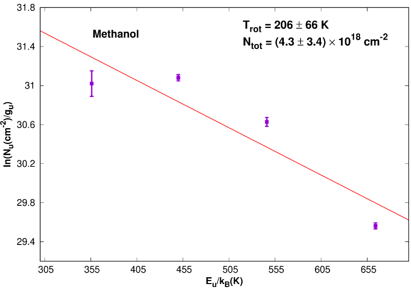
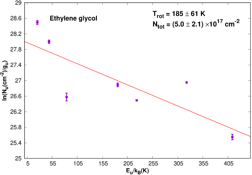
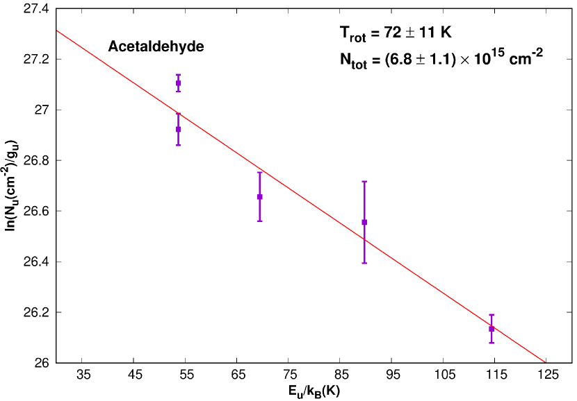
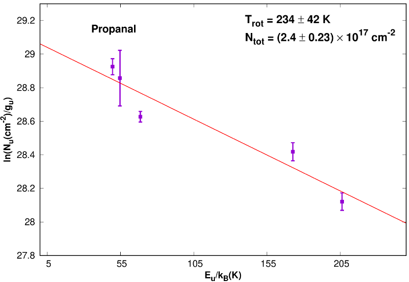
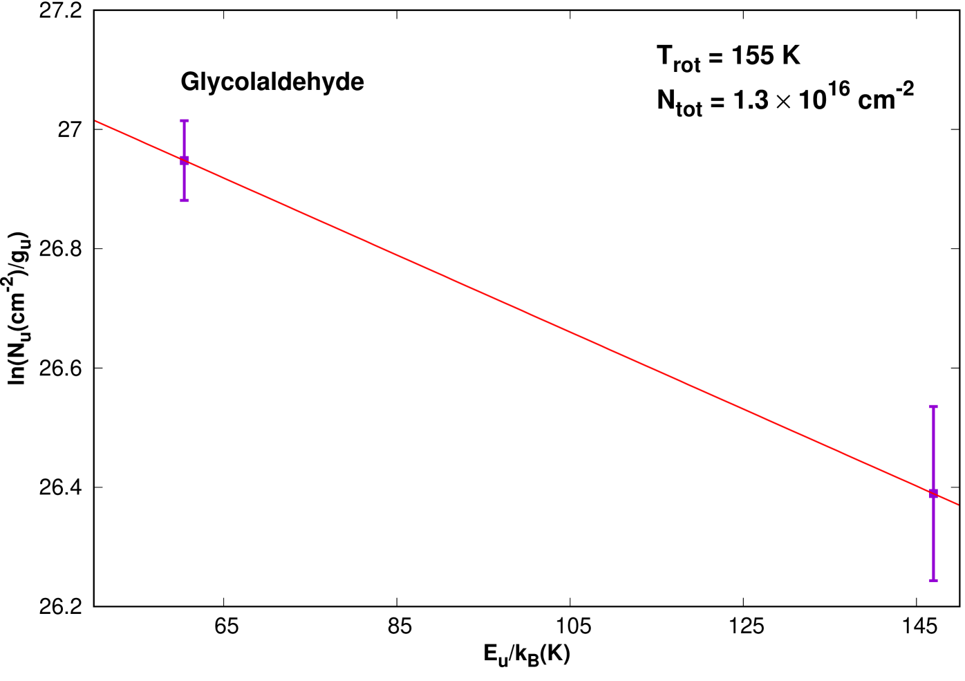
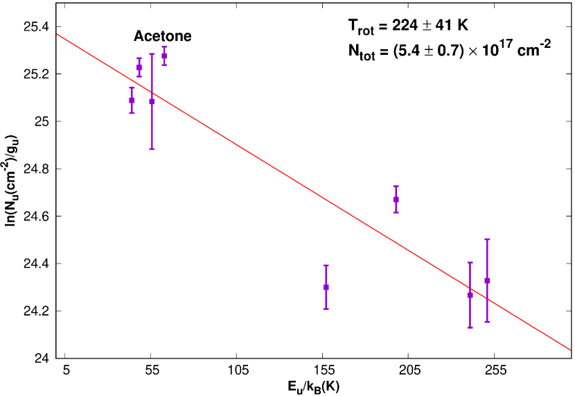
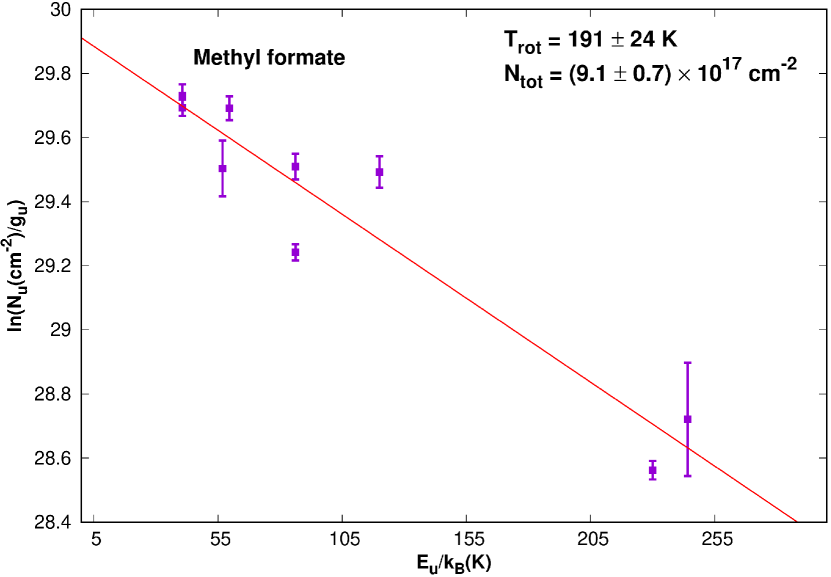
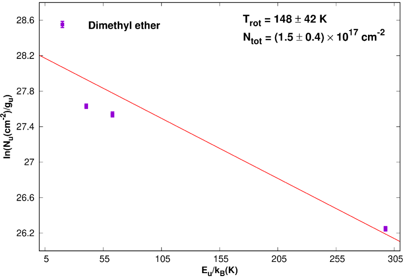
Figure 1: Rotation diagram of observed molecules are shown. The best fitted rotational temperature and column density are given in each panel. Filled purple squares are the data points and purple line represents the error bar.

2.5 Rotation diagram analysis

Here, a rotational diagram analysis is performed by assuming the observed transitions are optically thin and in Local Thermodynamic Equilibrium (LTE). For optically thin lines, column density can be expressed as (Goldsmith & Langer, 1999),

$$\frac{N_{u}^{thin}}{g_{u}}=\frac{3k_{B}\int{T_{mb}dV}}{8\pi^{3}\nu S\mu^{2}},$$ (1)

where, g_u is the degeneracy of the upper state, $k_{B}$ is the Boltzmann constant, $\rm{\int T_{mb}dV}$ is the integrated intensity, $\nu$ is the rest frequency, $\mu$ is the electric dipole moment, and S is the line strength. Under LTE condition, the total column density would be written as,

$$\frac{N_{u}^{thin}}{g_{u}}=\frac{N_{total}}{Q(T_{rot})}\exp^{-E_{u}/k_{B}T_{rot}},$$ (2)

where, $T_{rot}$ is the rotational temperature, E_u is the upper state energy, $\rm{Q(T_{rot})}$ is the partition function at rotational temperature. The above two equations can be rearranged as,

$$ln\Bigg{(}\frac{N_{u}^{thin}}{g_{u}}\Bigg{)}=-\Bigg{(}\frac{1}{T_{rot}}\Bigg{)}\Bigg{(}\frac{E_{u}}{k_{B}}\Bigg{)}+ln\Bigg{(}\frac{N_{total}}{Q(T_{rot})}\Bigg{)}.$$ (3)

The rotational temperature and total column density of a species are simultaneously determined from this expression. All the spectroscopic parameters for this analysis are taken either from the Cologne Database for Molecular Spectroscopy (CDMS, https://cdms.astro.uni-koeln.de, Müller et al., 2001, 2005; Endres et al., 2016) or from the Jet Propulsion Laboratory datebase (JPL, http://spec.jpl.nasa.gov, Pickett et al., 1998). Rotational diagram of methanol (CH₃OH), acetaldehyde (CH₃CHO), ethylene glycol [(CH₂OH)₂], glycolaldehyde (HOCH₂CHO), propanal (CH₃CH₂CHO), acetone (CH₃COCH₃), methyl formate (CH₃OCHO), and dimethyl ether (CH₃OCH₃) are shown in Figure 1. The derived rotational temperatures and column densities are summarized in Table 2. In Table 2, we have noted the errors. The relative percentage errors of the rotational temperature and column density are noted at the footnote of the table. The rotational diagram of glycolaldehyde is constructed with only two data points. Therefore, the rotational temperature has been assumed to some constant value. Methanol transitions with a wide range (166 K - 664 K) of upper state energies are observed. Some of these transitions are optically thick (i.e., $153.281$ GHz and $154.425$ GHz). Therefore, it is challenging to construct the rotation diagram with all seven unblended methanol lines (noted in Table 1). Since two transitions are optically thick, these are excluded from the rotation diagram analysis. Furthermore, by considering the rest of the five transitions, considerable uncertainty in the estimated column density ($(3.7\pm 3)\times 10^{18}$ cm^-2) and rotational temperature ($345\pm 198$ K) is obtained. Comparatively, a better linear fit was possible if we exclude the $148.111$ GHz transitions from the rotation diagram (by choosing the transitions having upper state energy $>300$ K). It yields a column density and rotational temperature of methanol ($4.3\pm 3.4)\times 10^{18}$ cm^-2 and $206\pm 66$ K, respectively.

For the sample of considered molecules, our estimated rotation temperature varies from $72$ K to $234$ K. A low rotation temperature $\sim 72\pm 11$ K for acetaldehyde is obtained, which is in agreement with the rotation temperature of accetaldehyde obtained by Ikeda et al. (2001). Olmi et al. (1996) derived a temperature of 160 K for CH₃CN. Rolffs et al. (2011) considered a temperature of 200 K to give an optimum fit to the data for line identification purposes. The average rotational temperature obtained from the species observed here is $177$ K, which is in close agreement with Olmi et al. (1996); Rolffs et al. (2011). There could be a possibility of beam dilution on the derived column densities and excitation temperatures. If the beam dilution effect is included in the rotation diagram, it is noticed that, on average, our column densities and temperatures would increase by a factor of $3.2$ and $1.4$, respectively. Derived column density and rotational temperature are further used in the LTE module of CASSIS to produce synthetic LTE spectra and also compare with our observations (see Figure 7). The average FWHM of each species from Table 1 is used for this computation. A source size of 2${}^{{}^{\prime\prime}}$ with the ALMA telescope is considered. Figure 7 shows a good agreement with the observed feature except for the three transitions of methanol and all the transitions of dimethyl ether. The intensity of the three methanol transitions is overproduced. Among them, $153.281$ GHz and $154.425$ GHz transitions are optically thick. All the transitions of dimethyl ether are underproduced. During the line analysis, it is noticed that these transitions consist of multiple sub-states. The strongest transition is only considered based on their S$\mu^{2}$ value. Thus, the obtained FWHMs are possibly overestimated during the Gaussian fitting, which can under-produce the intensity of these transitions in Figure 7.

Table 3: Calculated Gibbs free energy of activation, activation barrier, and reaction enthalpy of alochols formation via successive hydrogen addition with aldehydes, ketone, and ketene by using lower-level [B3LYP/6-31+G(d,p)] and higher-level [CCSD(T)/aug-cc-pVTZ] of theory considering $298.15$ K temperature and $1$ atmospheric pressure.

Serial No.	Reaction type	Reactions	Gibbs Free Energy of Activation		Activation Barrier		Enthalpy of Reaction
			(kcal/mol)		(kcal/mol)		(kcal/mol)
			Gas Phase	Ice Phase	Gas Phase	Ice Phase	Gas Phase	Ice Phase
Methanal - Methanol
1a.	(NR)	H2CO + H $\rightarrow$ CH2OH	10.57	11.32	5.59 (9.35)a[10.35]i	6.49 (10.02)a[11.16]i	-32.31	-32.39
1b.	(RR)	CH2OH + H $\rightarrow$ CH3OH	$\cdots$	$\cdots$	0.00	0.00	-94.75	-94.93
2a.	(NR)	H2CO + H $\rightarrow$ CH3O	7.10	6.97	1.89 (3.35)a[4.29]i	1.76 (3.10)a[3.26]i	-27.61	-27.07
2b.	(RR)	CH3O + H $\rightarrow$ CH3OH	$\cdots$	$\cdots$	0.00	0.00	-99.44	-100.24
Ethanal - Ethanol
3a.	(NR)	CH3CHO + H $\rightarrow$ CH3CHOH	11.41	12.44	5.91 (9.38)a	6.91 (10.24)a	-27.96	-26.80
3b.	(RR)	CH3CHOH + H $\rightarrow$ CH3CH2OH	$\cdots$	$\cdots$	0.00	0.00	-92.61	-93.21
4a.	(NR)	CH3CHO + H $\rightarrow$ CH3CH2O	10.10	10.24	4.11 (5.36)a	4.25 (5.38)a	-21.50	-20.27
4b.	(RR)	CH3CH2O + H $\rightarrow$ CH3CH2OH	$\cdots$	$\cdots$	0.00	0.00	-99.07	-99.74
Propanal - 1-Propanol
5a.	(NR)	CH3CH2CHO + H $\rightarrow$ CH3CH2CHOH	11.12	12.08	5.47 (9.27)a[9.82]ii	6.41 (9.87)a	-28.10 [-26.31]ii	-18.42
5b.	(RR)	CH3CH2CHOH + H $\rightarrow$ CH3CH2CH2OH	$\cdots$	$\cdots$	0.00	0.00	-92.82	-101.80
6a.	(NR)	CH3CH2CHO + H $\rightarrow$ CH3CH2CH2O	10.08	10.27	3.99 (4.97)a[5.71]ii	4.19 (4.96)a	-22.00 [-19.74]ii	-20.76
6b.	(RR)	CH3CH2CH2O + H $\rightarrow$ CH3CH2CH2OH	$\cdots$	$\cdots$	0.00	0.00	-98.91	-99.46
Propenal - Allyl alcohol
7a.	(NR)	CH2CHCHO + H $\rightarrow$ CH2CHCHOH	9.56	10.48	4.00(6.30)a[7.89]ii	2.36 (10.47)a	-40.29 [-38.93]ii	-39.59
7b.	(RR)	CH2CHCHOH + H $\rightarrow$ CH2CHCH2OH	$\cdots$	$\cdots$	0.00	0.00	-76.72	-77.07
8a.	(NR)	CH2CHCHO + H $\rightarrow$ CH2CHCH2O	10.32	10.24	4.43 (5.79)a[6.43]ii	4.38 (6.60)a	-18.00 [-16.16]ii	-16.72
8b.	(RR)	CH2CHCH2O + H $\rightarrow$ CH2CHCH2OH	$\cdots$	$\cdots$	0.00	0.00	-99.00	-99.95
Propynal - Propargyl alcohol
9a.	(NR)	HC2CHO + H $\rightarrow$ HC2CHOH	8.86	9.65	3.41 [7.41]ii	4.20 (8.28)a	-43.92 [-42.42]ii	-43.22
9b.	(RR)	HC2CHOH + H $\rightarrow$ HC2CH2OH	$\cdots$	$\cdots$	0.00	0.00	-79.53	-80.44
10a.	(NR)	HC2CHO + H $\rightarrow$ HC2CH2O	9.63	9.47	3.74 [5.78]ii	3.59 (5.68)a	-22.42 [-21.00]ii	-22.20
10b.	(RR)	HC2CH2O + H $\rightarrow$ HC2CH2OH	$\cdots$	$\cdots$	0.00	0.00	-101.02	-101.46
Glycolaldehyde - Ethylene glycol
11a.	(NR)	HOCH2CHO + H $\rightarrow$ HOCH2CHOH	11.42	12.31	5.50 (8.75)a[9.51]iii	6.32 (9.29)a	-29.43	-30.43
11b.	(RR)	HOCH2CHOH + H $\rightarrow$ HOCH2CH2OH	$\cdots$	$\cdots$	0.00	0.00	-92.18	-92.44
12a.	(NR)	HOCH2CHO + H $\rightarrow$ HOCH2CH2O	9.43	9.67	3.34 (4.47)[4.97]iii	3.38 (4.17)a	-22.38	-22.61
12b.	(RR)	HOCH2CH2O + H $\rightarrow$ HOCH2CH2OH	$\cdots$	$\cdots$	0.00	0.00	-99.22	-100.25
Acetone - Isopropanol
13a.	(NR)	CH3COCH3 + H $\rightarrow$ CH3COHCH3	11.27	12.44	5.56 (9.15)a	6.66 (9.85)a	-25.76	-24.35
13b.	(RR)	CH3COHCH3 + H $\rightarrow$ CH3CHOHCH3	$\cdots$	$\cdots$	0.00	0.00	-90.73	-91.08
14a.	(NR)	CH3COCH3 + H $\rightarrow$ CH3CHOCH3	12.97	12.97	6.29	6.55 (—)b	-16.40	-24.35
14b.	(RR)	CH3CHOCH3 + H $\rightarrow$ CH3CHOHCH3	$\cdots$	$\cdots$	0.00	0.00	-100.10	-91.08
Ethenone - Vinyl alcohol
15a.	(NR)	CH2CO + H $\rightarrow$ CH2COH	17.52	18.22	11.80 (5.39)	12.49 (17.59)a	-15.60	-16.96
15b.	(RR)	CH2COH + H $\rightarrow$ CH2CHOH	$\cdots$	$\cdots$	0.00	0.00	-45.67	-45.30
16a.	(NR)	CH2CO + H $\rightarrow$ CH2CHO	10.04	9.92	4.36 (3.97)	4.26 (5.43)a	-41.76	-43.87
16b.	(RR)	CH2CHO + H $\rightarrow$ CH2CHOH	$\cdots$	$\cdots$	0.00	0.00	-19.51	-18.40

Note. — NR refers to Neutral-Radical reactions, and RR to Radical-Radical reactions.

^aBracketed values are calculated using CCSD(T)/aug-cc-pVTZ level, ^bWe did not find true transition state, ⁱSong & Kästner (2017), ⁱⁱZaverkin et al. (2018), ⁱⁱⁱÁlvarez-Barcia et al. (2018).

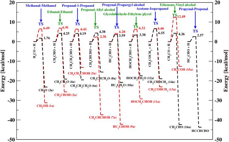
Figure 2: Schematic potential energy surfaces of alcohol formation from aldehyde and ketone for various hydrogenation reactions (representing IEFPCM correction for the influence of ice) indicating stable species and transition states. Energy differences in units of kcal/mol are shown, referenced to reactant complexes calculated using DFT-B3LYP/6-31G+(d,p) level of theory. The red lines denote H addition at O positions, whereas the black lines represent H addition at C positions.

3 Kinetics of the aldehydes, alcohols, ketone, and ketene observed in G10

Here, an extensive theoretical investigation is carried out to understand the formation mechanism of some aldehydes, alcohols, ketene, and ketone, which are observed in G10. All the quantum chemical results presented in this article are carried out using the Gaussian 09 suite of programs (Frisch et al., 2013). The Density Functional Theory (DFT) method with B3LYP functional (Becke, 1993) and 6-31+G(d,p) basis set is used in computing the activation barrier and enthalpy of reactions. Both the activation and reaction energies are calculated including the harmonic zero-point vibrational energy (ZPVE) and considering a temperature of $\sim 298.15$ K and $\sim 1$ atmosphere pressure. A fully optimized ground-state structure is verified to be a stationary point (having non-imaginary frequency) by harmonic vibrational frequency analysis. For the transition state (TS) calculation, the QST2 method of the Gaussian 09 program is used. All the TSs are verified using the internal reaction coordinate (IRC) analysis which connects reactants and products through the minimum energy path of the potential energy surface (PES). Further, the higher-order method is employed to examine the effect on the activation barrier calculation. The single point energy calculation of the TS structure and the optimized structure of the reactants at CCSD(T)/aug-cc-pVTZ level is carried out. The ice mixture is considered embedded within a continuum solvation field to include the passive impact of bulk ice on the activation barrier and enthalpy of reaction. To mimic the ice phase feature, water is used as the solvent. A self-consistent reaction field (SCRF) is routinely applied in the electronic structure calculations to study the spectroscopy and thermochemistry parameters of any species in the ice phase. Explicit water molecules can also generate a more realistic (inhomogeneous) field. Since the typical size of the interstellar water cluster (numbers of water molecules required) is not known with certainty, it is preferred to use the SCRF method (Woon, 2002b). The Polarizable Continuum Model (PCM) with different integral equation formalism variant (IEFPCM) as a default self-consistent reaction field (SCRF) method is used for this purpose (Cancès et al., 1997; Tomasi et al., 2005). A similar level of theory and basis set is used for the gas phase calculations. This method creates a solute cavity by overlapping spheres (Tomasi & Persico, 1994; Pascual-Ahuir et al., 1987). The implicit solvation model places the molecule of interest inside a cavity in a continuous homogeneous dielectric medium (in this case, water) that represents the solvent. This method is proven to be producing convincing results for ices. The PCM model is used to consider the reaction field of bulk ice. Here, the cluster is treated explicitly to avoid spurious boundary effects. In this framework, the reaction fields issuing from a dielectric constant of $78$ for water or about 100 for ice (Aragones et al., 2011) are essentially identical. Hence, the solid phase calculations and the thermochemistry parameters reported here are close to those in ice. The BE and PA of the aldehydes, ketone, ketene, and corresponding alcohols are also calculated quantum chemically discussed in Section 3.2.

3.1 Rate constants

A cross-over temperature, T_c is defined as the maximum temperature below which tunneling reaction dominates and above which thermal activation reaction takes over. T_c is calculated by the following relation:

$$T_{c}=\frac{h\omega}{4\pi^{2}k_{B}},$$ (4)

where h is the Planck’s constant, k_B is the Boltzmann constant, and $\omega$ is the absolute value of the the imaginary frequency at the TS. For all the gas phase reactions, the transition state theory (TST) is applied. Gas-phase rate constant can be calculated by the following expression,

$$K=\Big{(}\frac{k_{B}T}{hc^{0}}\Big{)}\exp(-\Delta{G}^{{\ddagger}}/RT),$$ (5)

where, $\rm{\Delta{G}^{{\ddagger}}}$ is the Gibbs free energy of activation, $c^{0}$ is the concentration ($\sim 1$), $R$ is the ideal gas constant and $T$ is the temperature.

High-level quantum chemical calculations of six aldehyde-alcohol pairs with one ketone-alcohol and one ketene-alcohol pairs are presented and discussed in detail. Aldehyde to alcohol, ketone to alcohol, ketene to alcohol formation may occur through successive hydrogen addition reaction in two steps: The first step is aldehyde/ketone/ketene + H $\rightarrow$ radical-1 and the second step is radical-1 + H $\rightarrow$ alcohol. The first step of all these reactions is neutral-radical reactions, whereas the second step is a radical-radical reaction. The first step of all these reactions thus having an activation barrier, whereas the second step is barrierless as both reactants have free electrons, which makes them very reactive. Our calculations show that six aldehydes (such as methanal, ethanal, propanal, propenal, propynal, and glycolaldehyde), one ketone (such as acetone), and one ketene (such as ethenone) are forming alcohols (such as methanol, ethanol, 1-propanol, allyl alcohol, propargyl alcohol, ethylene glycol, isopropanol, and vinyl alcohol, respectively) via two successive hydrogen addition reactions. In terms of stability, the observed alcohols are thermodynamically favorable compared to their isomers. The formation of complex molecules on the grain surface through successive hydrogen additions is found to be dominant. Formation pathways of these molecules are discussed below, and a graphical representation of PESs of their formation mechanism considering IEFPCM model and DFT-B3LYP/6-31G+(d,p) level of theory is shown in Figure 2.

3.1.1 Methanal and Methanol

Here, the activation barrier of the reaction H +H₂CO is computed, for the production of $\rm{CH_{2}OH}$ or $\rm{CH_{3}O}$ (reactions 1a and 2a of Table 3). It is noticed that the hydrogen addition to the carbon atom of H₂CO (i.e., the formation of CH₃O, methoxy radical) is more favorable than that of its addition to the O atom of H₂CO (i.e., the formation of CH₂OH) in both gas- and ice-phases considering both (DFT-B3LYP/6-31+G(d,p) and CCSD(T)/aug-cc-pVTZ) level of theory. This is consistent with earlier experimental and theoretical results (Chuang et al., 2016; Song & Kästner, 2017). Song & Kästner (2017) studied the TS of reactions 1a and 2a both in gas-phase and on five different binding sites of the amorphous solid water (ASW) surface and calculated the corresponding activation energies. We compare our activation energy values with their gas-phase and ice-phase for binding site ASW 5 in Table 3, which shows a good agreement when we considered CCSD(T)/aug-cc-pVTZ level of theory. Woon (2002a) predicted the barrier height of reaction 2a as 5.04 kcal/mol for the gas-phase and it decreases to 4.81 kcal/mol when the reaction is embedded with the IPCM field. In our case, we also found the similar decreasing trend from gas-phase to ice-phase considering both level of theory. Song & Kästner (2017) also computed the BE of H₂CO for different sites of amorphous solid water (ASW) surface and found that BE values vary between $1000$ K and $9370$ K. This uncertainty in the BE value may lead to a very different abundance of CH₃OH under different astrophysical environments. The hydrogen abstraction reaction of methanol also plays an essential role in controlling the abundance of COMs. Methanol abstraction reaction barrier and the rate constant are taken from Song & Kästner (2017).

3.1.2 Ethanal and Ethanol

Here, the formation of $\rm{C_{2}H_{5}OH}$ via two successive hydrogen addition reactions with the CH₃CHO is considered. Kinetic information (i.e., activation barrier and reaction enthalpy) of these two reactions are noted in Table 3. Looking at the activation barriers reported in Table 3, it is clear that similar to methanol formation, here also, the hydrogen addition at the carbon atom position of CH₃CHO (i.e., the formation of CH₃CH₂O, reaction 4a) is more efficient compared to the hydrogen addition at the O atom position (i.e., the formation of CH₃CHOH, reaction 3a). The relative abundances between the acetaldehyde and ethyl alcohol seem to depend upon the evolution time, availability of the hydrogen atoms, ice thickness, and ice morphology (Bisschop et al., 2007, 2008). Only the hydrogenation reactions are not enough in explaining the observed abundances of ethanal-ethanol. It is needed to consider the ice phase reaction between CH₃ and CH₂OH for the formation of ethanol in the ice phase.

3.1.3 Propanal and 1-Propanol

The coexistence of propanal, propynal, and propenal in Sgr B2(N) (Hollis et al., 2004) could be explained by the following successive hydrogenation sequences; $\rm{HC_{2}CHO\ (propynal)\ \rightarrow\ CH_{2}CHCHO\ (propenal)}$ $\rm{\rightarrow\ CH_{3}CH_{2}CHO\ (propanal)}$. Recently, Qasim et al. (2019) studied the propanal formation by the radical-radical reaction between HCO and $\rm{H_{3}CCH_{2}}$. They used the sequential hydrogenation of propanal to form 1-propanol. The first step of the reaction has a high activation barrier. But this reaction can change the saturated bond to the unsaturated radicals, which may again undergo some radical-radical recombination reactions. Qasim et al. (2019) obtained a significant production of 1-propanol with this pathway. Our TST calculation for the successive hydrogenation pathways is shown in Table 3. It is noticed that the hydrogen addition at the carbon atom position of propanal ($\rm{CH_{3}CH_{2}CH_{2}O}$ formation, reaction 6a of Table 3) is favorable compared to the oxygen atom position of propanal ($\rm{CH_{3}CH_{2}CHOH}$ formation, reaction 5a). The gas-phase activation and reaction energies (including ZPVE) of Zaverkin et al. (2018) are compared with ours in Table 3 which is in good agreement with our values calculated using higher-level of theory. Except the successive hydrogenation reactions, following ice phase reactions, are also considered for the formation of propynal, propenal, and propanal.

$${\rm C_{2}H+H_{2}CO\rightarrow propynal+H},$$

$${\rm O+C_{3}H_{3}\rightarrow propynal+H},$$

$${\rm HCO+C_{3}H_{3}\rightarrow propenal+H},$$

$${\rm HCO+H_{3}CCH_{2}\rightarrow propanal+H}.$$

3.1.4 Propenal and Allyl Alcohol

Propenal is also a product of the two successive hydrogenation reactions with propynal.

$${\rm propynal+2H\rightarrow propenal\ (CH_{2}CHCHO).}$$

Here, the other product channel of this reaction is studied. Firstly, the hydrogenation reaction of propynal would form propenal. In the second step, propenal could undergo another hydrogenation reaction to form allyl alcohol. The TS calculation of the first step found an activation barrier of 2.60 kcal/mol in the gas phase and 2.57 kcal/mol in the ice phase considering lower-level of theory (see Figure 2). Table 3 shows the activation barriers for the hydrogen addition at the propenal’s carbon and oxygen atom position. It is noted that, unlike the other cases, here, the hydrogen addition at the oxygen atom of propenal ($\rm{CH_{2}CHCHOH}$ formation, reaction 7a) seems to be more favorable than it is with the carbon atom position ($\rm{CH_{2}CHCH_{2}O}$ formation, reaction 8a) considering lower-level of theory. But considering higher-level of theory, opposite trend is found which agrees well with the values calculated by Zaverkin et al. (2018) shown in Table 3 for comparison.

3.1.5 Propynal and Propargyl Alcohol

Transformation from propynal ($\rm{HC_{2}CHO}$) to propargyl alcohol was already reported by Gorai et al. (2017b). This happened via two successive hydrogenations with propynal :

$${\rm propynal+2H\rightarrow propynol\ (propargyl\ alcohol,\ HC_{2}CH_{2}OH).}$$

Table 3 shows a different trend for the hydrogen addition for reactions 9a and 10a in the gas-phase. The hydrogen addition to the oxygen atom position (reaction 9a) is favorable than that of the carbon atom position (reaction 10a) using lower-level of theory, whereas Zaverkin et al. (2018) found an opposite trend. In contrast, the opposite trend is noticed for the ice-phase using both lower- and higher-level of theory.

3.1.6 Glycolaldehyde and Ethylene Glycol

Glycolaldehyde is the simplest form of the aldose family. The sugars like glucose, ribose, and erythrose belong to this family. Therefore, the presence of glycolaldehyde in space is an indication of the precursor of biologically relevant molecules. Identification of the numerous complex organic molecules in the Galactic Centre (GC) makes it an active area of research. Specifically, the study of the chemical evolution of the grain mantle, where various energetic processes (like UV radiation, X-rays, and cosmic rays, etc.) may reprocess the mantle composition, are fascinating. The C and O addition to the formyl radical and then three successive hydrogen additions yield glycolaldehyde. The two subsequent hydrogen additions to the glycolaldehyde can produce ethylene glycol (Charnley, 2001). Fedoseev et al. (2015) proposed that two HCO radicals can recombine to produce glyoxal (HC(O)CHO), which can also subsequently convert to glycolaldehyde. Coutens et al. (2018) investigated the formation mechanism of these two species (glycolaldehyde and ethylene glycol) using a gas-grain chemical model. They studied the EG/GA ratio for various luminosities. Álvarez-Barcia et al. (2018) studied two successive hydrogen addition reactions with acetaldehyde which can produce ethylene glycol. They also studied the hydrogen abstraction reactions of GA and EG. Table 3 shows the kinetics involved in converting ethylene glycol from glycolaldehyde. Like the methanal-methanol, ethanal-ethanol, propanal-1-propanol, and ice phase pathways of propynal-propargyl alcohol pairs, the favorable position of the hydrogen addition is noted to be the carbon atom ($\rm{HOCH_{2}CH_{2}O}$ formation, reaction 12a) instead of the oxygen atom ($\rm{HOCH_{2}CHOH}$ formation, reaction 11a) of glycolaldehyde.

3.1.7 Acetone and Isopropanol

Acetone ($\rm{CH_{3}COCH_{3}}$, propanone) and isopropanol ($\rm{CH_{3}CHOHCH_{3}}$, isopropyl alcohol, 2-propanol) might be chemically connected. Table 3 shows the two successive hydrogenations of acetone (reactions 13 and 14). We check the TST calculations for the hydrogen addition either with the oxygen atom (activation energy 5.56 kcal/mol) or with the carbon atom (activation energy 6.29 kcal/mol) position of acetone and found that the former one is more favorable than the latter in the gas phase considering lower-level of theory. In contrast, the opposite trend was noted in the ice phase. We could not find a proper TS using higher-level of theory for reaction 14a in the ice-phase.

3.1.8 Ethenone and Vinyl Alcohol

Vinyl alcohol is a planar molecule, which has two conformations. The “syn” conformer is found to be more stable than that of the “anti” conformer (Turner & Apponi, 2001). Here also, the “syn” conformer of vinyl alcohol is considered for the quantum chemical calculations. Here, the TS of the two successive hydrogen addition reactions to ketene is examined for the formation of vinyl alcohol. The first step has an activation barrier, whereas the second step is a radical-radical reaction and is assumed to be barrierless. Vinyl alcohol can also form from acetaldehyde via the isomerization process (Käser et al., 2020). Table 3 depicts that the hydrogen addition at the carbon atom position is more favorable than the oxygen atom position of ethenone. Table 3 shows that the H addition to the O atom position of ketene (reaction 15a) requires a significantly higher activation barrier than the H addition to the O atom position of the other species (reactions 1a, 3a, 5a, 7a, 9a, 11a, 13a) reported here. It could be due to the change of the hybridization of C atom of ketene from sp (linear) to sp2 (bent) during the H addition reaction. On the other hand, there is no change of hybridization upon H addition to the other aldehyde, which requires only small structural change and thus, the activation energy could be small. Carr et al. (1968) studied the reaction of ketene with atomic H at room temperature where the reaction $\rm{H+H_{2}CCO\rightarrow CH_{3}CO^{*}\rightarrow CH_{3}+CO}$ occurs rather slowly (rate constant $1.3\times 10^{-13}$ cm³mol^-1s^-1), while neither $\rm{H+H_{2}CCO\rightarrow CH_{2}CHO}$ nor H abstraction occur very significantly.

Table 4: Calculated binding energy values of the aldehydes, alcohols, ketone and ketene considered in this work.

Species	Ground state	Binding Energy (Kelvin)
	used	CO monomer	CH3OH monomer	H2O monomer	H2O tetramer (scaled by 1.188)	Available
Methanal	Singlet	641	2942	2896	3242a (3851)	2050b, 4500 $\pm$ 1350c
Methanol	Singlet	1247	3227	3124	4368a (5189)	5534b, 5000 $\pm$ 1500c
Ethanal	Singlet	1015	1964	3189	3849a (4573)	2450b, 5400 $\pm$ 1620c
Ethanol	Singlet	873	3408	2824	5045 (5993)	6584b, 5400 $\pm$ 1620c
Propanal	Singlet	680	3679	3522	3396 (4034)	4500 $\pm$ 1350c
1-Propanol	Singlet	1298	3932	2609	4791 (5692)	$\cdots$
Propenal	Singlet	1043	3236	3170	3495 (4152)	5400 $\pm$ 1620c
Allyl Alcohol	Singlet	1381	3625	2958	5964 (7085)	$\cdots$
Propynal	Singlet	1174	3072	2318	3379 (4014)	$\cdots$
Propargyl Alcohol	Singlet	1031	4119	2870	4284 (5089)	$\cdots$
Glycolaldehyde	Singlet	826	3254	2871	5131 (6096)	$\cdots$
Ethylene Glycol	Singlet	933	4666	3144	4602 (5467)	$\cdots$
Acetone	Singlet	728	3769	3623	4420 (5251)	3500b
Isopropanol	Singlet	1369	3640	2879	5230 (6213)	$\cdots$
Ethenone	Singlet	732	1450	1317	2847 (3382)	2200b, 2800 $\pm$ 840c
Vinyl Alcohol	Singlet	1236	3407	2836	3786 (4497)	$\cdots$

Note. — ^aDas et al. (2018), ^bKIDA old BE, ^cKIDA new BE (Wakelam et al., 2017).

Table 5: Calculated proton affinity of these species.

Species	Protonation Reactions	Proton Affinity (kJ/mol)
		Our calculation	Available
Methanal	HCHO + H+ $\rightarrow$ CH2OH+	692	712.9 $\pm$ 1.1a
Methanol	CH3OH + H+ $\rightarrow$ CH3OH${}_{2}^{+}$	740	754.3a
Ethanal	CH3CHO + H+ $\rightarrow$ CH3CHOH+	749	768.5 $\pm$ 1.6a
Ethanol	C2H5OH + H+ $\rightarrow$ C2H5OH${}_{2}^{+}$	764
Propanal	CH3CH2CHO + H+ $\rightarrow$ HCH3CH2CHO+	769
1-Propanol	CH3CH2CH2OH + H+ $\rightarrow$ HCH3CH2CH2OH+	770
Propenal	CH2CHCHO + H+ $\rightarrow$ CH2CHCHOH+	764
Allyl Alcohol	CH2CHCH2OH + H+ $\rightarrow$ CH2CHCH2OH${}_{2}^{+}$	773
Propynal	$\rm{HC_{2}CHO+H^{+}\rightarrow HC_{2}CHOH^{+}}$	733
Propargyl Alcohol	$\rm{HC_{2}CH_{2}OH+H^{+}\rightarrow HC_{2}CH_{2}OH_{2}^{+}}$	742
Glycolaldehyde	HOCH2CHO + H+ $\rightarrow$ H2OCH2CHO+	759
Ethylene Glycol	HOCH2CH2OH + H+ $\rightarrow$ HOCH2CH2OH${}_{2}^{+}$	797
Acetone	CH3COCH3 + H+ $\rightarrow$ CH3COHCH${}_{3}^{+}$	793
Isopropanol	CH3CHOHCH3 + H+ $\rightarrow$ CH3CHOH2CH${}_{3}^{+}$	782
Ethenone	CH2CO + H+ $\rightarrow$ CH3CO+	822	825.3$\pm$3a
Vinyl Alcohol	CH2CHOH + H+ $\rightarrow$ CH3CHOH+	800	882.8b

Note. — ^aHunter & Lias (1998), ^bTurner & Apponi (2001)

Table 6: Comparison between the observed abundance and our CMMC results with Model C (set 4).

Species	Obtained abundances	Obtained abundance	Observed abundances
	from model	ratio from model	G31.41+0.31	Sgr B2 (N)	Orion KL	G10.47+0.03
Methanal	$3.3(-9)-5.8(-7)$		$[1.9(-7)]^{e}$	$[3.2(-08)]^{m}$		$[6.1(-7)]^{b}$
Methanol	$3.5(-8)-1.4(-5)$	$1.0(1)-5.3(1)$	$[1.9(-6)]^{e}$	$[7.7(-7)]^{m}$ $[7.1(-6)]^{x}$	$[2.2(-7)]^{l}$	$[3.2\pm 2.5(-7)]^{a}$, $[1.8(-6)]^{b}$
Ethanal	$1.8(-13)-5.0(-9)$		$[1.0(-9)]^{n}$	$[1.4(-08)]^{m}$ $[9.5(-8)]^{x}$		$[5.0\pm 0.8(-10)]^{a}$
Ethanol	$7.4(-10)-9.7(-8)$	$8.0(-2)-2.6(4)$	$[2.0(-8)]^{n}[1.3(-9)]^{f}$	$[1.1(-7)]^{m}[3.6(-7)]^{x}$	$[1.3(-8)]^{l}$	$[1.2(-7)]^{b}$
Propanal	$7.3(-10)-4.8(-8)$					$[1.8\pm 0.2(-8)]^{a}$
1-Propanol	$2.4(-12)-1.1(-7)$	$2.6(-4)-1.3(2)$
Propenal	$2.0(-13)-1.9(-9)$					$[1.2(-10)]^{*d}$
Allyl alcohol	$8.7(-15)-1.7(-9)$	$3.6(-2)-2.9(0)$
Propynal	$3.1(-11)-2.2(-09)$
Propargyl alcohol	$6.4(-15)-1.3(-11)$	$1.4(-4)-1.0(-2)$
Glycolaldehyde	$2.8(-15)-1.3(-06)$		$[8.3(-11)]^{f}$	$[3.2(-10)]^{m}$ $[1.9(-8)]^{x}$	$[1.5(-10)]^{l}$	[$9.6\pm 0.007(-10)]^{a}$
Ethylene glycol	$5.5(-17)-1.6(-5)$	$1.9(-2)-4.45(2)$	$[1.7(-10)]^{f}$	$4.1(-10)]^{m}$	$[2.3(-9)]^{l}$	$[3.7\pm 1.5(-8)]^{a}$
Acetone	$6.6(-14)-1.7(-8)$			$[2.6(-8)]^{m}$		$[4.0\pm 0.5(-8)]^{a},\ [1.0(-7)]^{b}$
Isopropanol	$1.2(-13)-4.4(-9)$	$9.7(-2)-7.4(3)$
Ethenone	$4.6(-13)-5.5(-9)$					$[8.0(-8)]^{b}$
Vinyl alcohol	$3.5(-11)-1.4(-8)$	$1.9(0)-7.7(1)$				$[{\leq}2.3(-9)]^{*d}$
Methyl formate	$2.3(-11)-1.3(-6)$		$[2.6(-9)]^{f}$	$[7.7(-8)]^{m}$ $[9.5(-8)]^{x}$	$[1.2(-7)]^{k}$	$[6.7\pm 0.5(-8)]^{a},\ [1.4(-7)]^{b}$
Dimethyl ether	$3.5(-9)-1.5(-7)$	$1.2(-1)-1.5(2)$	$[4.2(-9)]^{f}$	$[3.5(-7)]^{m}$	$[3.0(-7)]^{k}$	$[1.1\pm 0.3(-8)]^{a},[3.0(-7)]^{b}$

G31 observation:^e Gorai et al. (2021) (used ALMA with $\theta_{b}=0.98^{{}^{\prime\prime}}-1.19^{{}^{\prime\prime}}$ and $\rm N_{H_{2}}=1.53\times 10^{25}$ cm^-2), ^f Rivilla et al. (2017) (used SMA with $\theta_{b}=0.75^{{}^{\prime\prime}}-3.5^{{}^{\prime\prime}}$ and $\rm N_{H_{2}}=1.2\times 10^{26}$ cm^-2), ⁿ Nummelin et al. (1998) (used SEST and IRAM with $\theta_{b}=10^{{}^{\prime\prime}}$ and $\rm N_{H_{2}}=1.6\times 10^{23}$ cm^-2)
Sgr B2 observation: ^x Belloche et al. (2014) (used ALMA with $\theta_{b}=1.2^{{}^{\prime\prime}}-1.9^{{}^{\prime\prime}}$ and $\rm N_{H_{2}}=5.6\times 10^{24}$ cm^-2), ^m Belloche et al. (2013) (used IRAM with $\theta_{b}=10^{{}^{\prime\prime}}-25^{{}^{\prime\prime}}$ and $\rm N_{H_{2}}=5.6\times 10^{24}$ cm^-2 (Belloche et al., 2014))
Orion KL observation: ^l Brouillet et al. (2015) (used ALMA with $1.4^{{}^{\prime\prime}}-1.9^{{}^{\prime\prime}}$ and $\rm{N_{H_{2}}=2.0\times 10^{24}}$ cm^-2 (Favre et al., 2011)), ^k Tercero et al. (2015) (used ALMA with $1.29^{{}^{\prime\prime}}-2^{{}^{\prime\prime}}$ and $\rm N_{H_{2}}=2.0\times 10^{24}$ cm^-2 (Favre et al., 2011))
G10 observation: ^a This work (used ALMA with $\theta_{b}=1.39^{{}^{\prime\prime}}-2.44^{{}^{\prime\prime}}$ and $\rm N_{H_{2}}=1.35\times 10^{25}$ cm^-2),^b Rolffs et al. (2011) (used SMA with $\theta_{b}=0.28^{{}^{\prime\prime}}-4.27^{{}^{\prime\prime}}$ and with $\rm N_{H_{2}}=5\times 10^{24}$ cm^-2),^∗d Dickens et al. (2001) (used SEST & NRAO for possible detection of propenal and upper limit for vinyl alcohol with $\theta_{b}=45^{{}^{\prime\prime}}$ and $\rm N_{H_{2}}=10^{23}$ cm^-2)

Note. —

3.2 Binding Energy and Proton Affinity

A sizable portion ($\sim 60-70\%$ of the surface coverage) of the interstellar icy layers may contain water molecules. That is why the BE of the interstellar species is usually explored with the H₂O surface. However, the rest ($\sim 30-40\%$) of the grain mantle would comprise other impurities. CO₂, CO, and CH₃OH can occupy a sizable portion of the grain mantle in different lines of sight. Keane et al. (2001) summarized the relative abundance of CO, CO₂, and CH₃OH relative to water ice could vary in the range of $0.4-15$, $0.17-21$, and $1.5-30$, respectively, in different lines of sight. So, the BE with these surface species is also important in the various evolutionary phases. It is needed to construct a model which can consider the BE depending on the surface composition of the ice. Furuya & Persson (2018) reported a model in which the BE depends on the surface composition of ice mantles. However, showing the results of such a chemical model is out of scope for this work.

A realistic estimation of the BEs with various substrates is not available. In the absence of any experimental values, the quantum chemical method provides an educated estimate (Das et al., 2018; Wakelam et al., 2017). Here, CO and CH₃OH molecules are considered a substrate for this purpose.

Gaussian 09 suite of programs employed for the quantum chemical calculations is utilized to evaluate the BE values. To calculate the BE, which is opposite to interaction energy for the bound system, the optimized energy for the complex system (where a species is placed at a suitable distance from the grain surface) is subtracted from the total optimized energies of the grain surface and species. To find the optimized energy of all structures, a Second-order Møller-Plesset (MP2) method with an aug-cc-pVDZ basis set (Dunning, 1989) is used following Das et al. (2018). The ZPVE and basis set superposition error (BSSE) correction are not considered for BE calculations.

Obtained BE values are shown in Table 4. It is interesting to note that a higher BE for the alcohol is obtained in most cases than their corresponding aldehyde, ketone, or ketene. Obtained values with CO and CH₃OH significantly differ from that of water. In terms of average values, the BE values with water monomer is $\sim 2.85$ times higher than the CO monomer and $1.16$ times lower in comparison to CH₃OH monomer. Here, in our chemical model, the obtained BE values with CO and CH₃OH are not included because it is not available for the other species. However, BE values obtained with the c-tetramer water configuration are included in our model with an appropriate scaling factor suggested in Das et al. (2018). In Table 4, the ground state spin multiplicity of the species used to calculate the BE is also noted. Separate calculations (job type “opt+freq” in Gaussian 09 suite) with different spin multiplicities are used. The lowest energy electronic state in between these is noted as the ground state.

The protonation reactions (i.e., X + H⁺ $\rightarrow$ XH⁺) and proton transfer reactions (i.e., X + YH⁺ $\rightarrow$ XH⁺ + Y) have a significant impact on the interstellar chemistry (Wakelam et al., 2010; Herbst & Leung, 1986). The ab-initio quantum chemical approaches provide a reliable value of the proton affinity for small molecules where the experimental determination of these parameters is a difficult task. A systematic study to calculate the adiabatic PA of aldehydes, ketone, ketene, and corresponding alcohols is considered in this work. PA is defined as the energy released when a proton is added to a system. Thus the energy difference between a species and a species with an additional proton (H⁺) is estimated. It is calculated as the difference in energy (electronic + zero-point energy) between a neutral species and its protonated analog, i.e.,

$$PA=E_{X}-E_{XH^{+}},$$ (6)

where $\rm{E_{X}}$ is the optimized energy of the species X, and $\rm{E_{XH^{+}}}$ is the optimized energy of the protonated species, XH$+$. To find the optimized energy of all structures, a Second-order Møller-Plesset (MP2) method with an aug-cc-pVDZ basis set is again used. This is then verified via harmonic frequency calculations with the equilibrium geometries having only real frequencies. Zero-point correction to energies is not considered to evaluate the PA of the species reported here. The protonation of a neutral species can occur in more than one position, which yields different protonated species with other PA. To avoid any ambiguity, only the highest PA is noted in Table 5. Protonated form with higher PA of a neutral species is found to be more stable and more abundant (in some cases), and thus may be detectable. In contrast, another protonated form with lower PA forming from the same neutral species is less stable. This species is very reactive, and the high reactivity of this protonated species may reduces its interstellar abundance. We notice that ethenone has the highest and methanal has the lowest PA among all the species considered for this study.

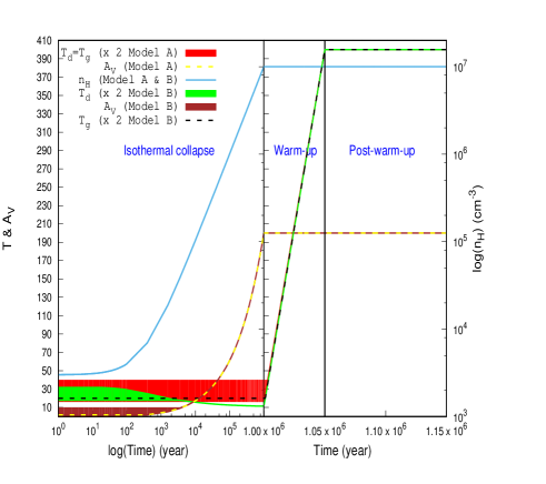
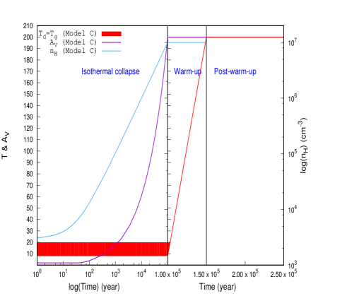
Figure 3: Physical conditions considered in Model A and Model B are shown in the upper panel and in the lower panel, we show the adopted physical conditions for Model C. The X-axis of the figure shows the logarithmic scale for the isothermal collapsing phase, whereas, beyond that, it is shown on the regular scale. In case of Model A and Model C, an isothermal collapsing phase is considered whereas in Model B, a pre-stellar core phase is considered where temperature is decreased in the upper panel, temperature is scaled by a factor of 2 for the better visibility.

4 Chemical modeling

The Chemical Model for Molecular Cloud (hereafter CMMC) (Das et al., 2015a, b, 2019, 2021; Gorai et al., 2017a, b; Sil et al., 2018; Bhat et al., 2021; Gorai et al., 2020; Sil et al., 2021) is implemented for studying the formation of aldehydes, ketone, ketene and their corresponding alcohols. The low metallic elemental abundances are used as the initial abundances (Wakelam & Herbst, 2008, EA1 set). Gas-phase pathways of CMMC are mainly adopted from the UMIST database (McElroy et al., 2013). Additionally, a complete network for the formation of alcohols and aldehydes is considered. For the construction of these reaction sets, the ice phase reactions noted in Table 3 are considered. The activation energy barriers calculated with the CCSD(T)/aug-cc-pVTZ level are adopted. Since, for the reaction 13a of Table 3, a true TS was not obtained with the CCSD(T)/aug-cc-pVTZ level of theory, the activation barrier obtained with the B3LYP/6-31+G(d,p) level of theory is used. For the gas phase destruction of these species, interstellar photoreactions, cosmic-ray induced reactions, and ion-molecular reactions with major ions (He⁺, $\rm{H_{3}}^{+}$, HCO⁺, H₃O⁺, C⁺, etc.) are considered. The destruction of some of these reactions was already available in McElroy et al. (2013). If it is not available, a very similar reaction with the same rate constants is adopted for these reactions. A cosmic ray rate of $1.3\times 10^{-17}$ s^-1 is considered in all our models. Cosmic ray-induced desorption and chemical desorption with the efficiency of $1\%$ is considered. For the all-grain surface species, a photodesorption rate of $3\times 10^{-3}$ per incident UV photon (Öberg et al., 2007) is adopted. A sticking coefficient of $1.0$ is considered for the neutral species. Sticking coefficients of H and H₂ is taken from Chaabouni et al. (2012). On the grain surface, the diffusive surface reaction can lead to chemical complexity. However, to successfully continue the diffusive reaction mechanism, the reactants should be in the close vicinity until they react. There is a possibility that two reactants can move apart or be desorbed back to the gas phase. So it is essential to consider the competition between diffusion, desorption, and reaction. Following Garrod & Pauly (2011), here this possibility is included. At the high density ($\sim 10^{7}$ cm^-3) and around $10$ K, a notable portion of the grain surface would be covered by molecular hydrogen. At this stage, encounter desorption of H₂ (Hincelin et al., 2015; Chang et al., 2021; Das et al., 2021) needs to be considered to avoid an unnecessary surge in the grain’s molecular hydrogen. The grain mantle’s chemical composition at this phase is crucial to delivering the surface species into the gas phase during the warm-up stage. Here, the encounter desorption mechanism of H₂ is considered in our model.

The BE ($E_{d}$) of the surface species plays a decisive role in controlling the chemical complexity of the interstellar ice. A straightforward relation between the diffusion energy ($E_{b}$) of a species with the BE is considered by following $E_{b}=RE_{d}$, where, R may vary in between $0.35-0.8$ (Garrod et al., 2007). Here, $R=0.35$ and $0.50$ are used to show their effects on the chemical complexity. These BEs are either taken from the KIDA database or taken from Das et al. (2018). Das et al. (2018) provided BE values for some relevant interstellar species with the water surface. They computed the interaction energies, varying the size of the substrate. They showed that their method would yield a minimum deviation with the experimentally obtained BE values when a higher-order cluster is used. Table 4 shows the computed BEs of these aldehydes, alcohols, ketone, and ketene with various substrates. The ground state used to calculate the BE of these molecules is also pointed out along with the BE values in Table 4. Das et al. (2018) suggested a scaling factor $\sim 1.188$ while using the tetramer water configuration for the computation of the BE. The scaled BE values are also noted in Table 4. Except for the glycolaldehyde and ethylene glycol pair, for all the cases, obtained BEs with the tetramer configuration are noted to be comparatively higher than that of their related aldehyde, ketone, or ketene. These new sets of BEs with the tetramer configuration of water molecules are included in our chemical model with appropriate scaling.

Depending on the BEs and R values, four sets of BEs are constructed (see Table 7). For set 1 and set 2, BEs are used from the KIDA database (Wakelam et al., 2017). The only difference between set 1 and set 2 is that for set 1, $R=0.5$ is used, whereas, for set 2, $R=0.35$ is used. Recently, Das et al. (2018) provided a set of BEs for $100$ relevant interstellar species with the water surface. They used the tetramer configuration of water molecules for this calculation. They suggested using a scaling factor of $1.188$ with this to estimate the BEs of these species. The set 3 is constructed with the BE values provided by Das et al. (2018). Sil et al. (2017) reported the BEs of H and H₂ for a comprehensive collection of surfaces (benzene, silica, and water). They showed that the BE of H and H₂ are very sensitive to the choice of substrates. These variations should be expected for all the species if various substrates would have been considered. But showing all the changes here would be out of scope for this work. Here, one additional BE set is considered, where the BE of H and H₂ are kept the same as it was used in KIDA, but for the others, it is the same as it is in set 3. Thus, in set 3, BE of H, and H₂ of 148 K, and 627 K, respectively, are used from Das et al. (2018) after scaling by 1.188, whereas in set 4, it is used 650 K and 440 K, respectively for H, and H₂ (Wakelam et al., 2017). $R=0.35$ is considered for both the set 3 and 4.

Table 7: Different sets of BE used based on the ratio between the diffusion energy to binding energy (R).

	BEs used	R
set 1	Wakelam et al. (2017)	0.5
set 2	Wakelam et al. (2017)	0.35
set 3	1.188 $\times$ BE of Das et al. (2018)	0.35
set 4	1.188 $\times$ BE of Das et al. (2018), BE of	0.35
	H, and H2 from Wakelam et al. (2017)

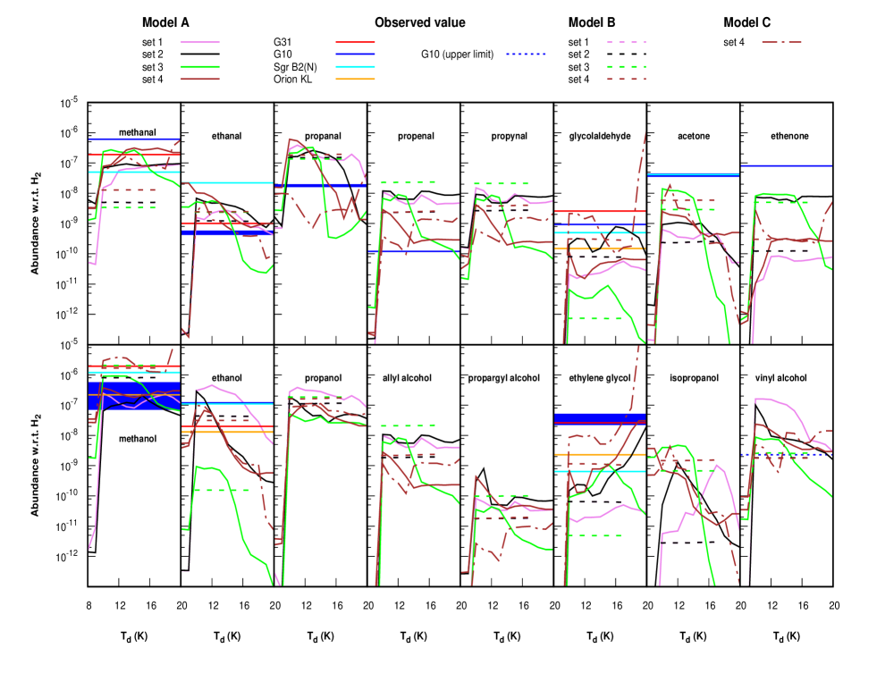
Figure 4: The initial dust temperature versus the peak gas-phase abundance obtained from Model A, Model B, and Model C is shown in various cases. Eight pairs of species are shown. Observed/upper-limit of the abundances of these species are marked with red (G31), blue (G10), Sgr B2(N) (cyan), and Orion KL (orange) if available. Since, in G10, some species are identified here, observed errors are shown with the thick blue curve. The solid curve represents the cases with Model A and dashed curves represent the same cases for Model B. Results obtained with Model C and set 4 are shown with the dashed-dot lines. The lower eight panels show the peak abundance variation of alcohols whereas the top panels show their related aldehyde, ketone, and ketene respectively. Thus, we conclude that there is both observational and theoretical evidence for production of alcohols via hydrogenation of precursor aldehydes, ketones and ketenes.

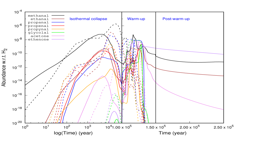
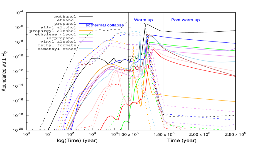
Figure 5: The chemical evolution of aldehyde, ketone, ketene and their corresponding alcohols are shown with the set 4 of CMMC Model C while initial dust temperature kept at $10$ K. The X-axis of the figure shows the logarithmic scale for the isothermal collapsing phase, whereas, beyond that, it is shown on the regular scale. Gas phase abundance are represented with the solid curve whereas for the ice phase it is with the dashed curve. Additionally, the time evolution of propynal, methyl formate, and dimetyhyl ether are shown.

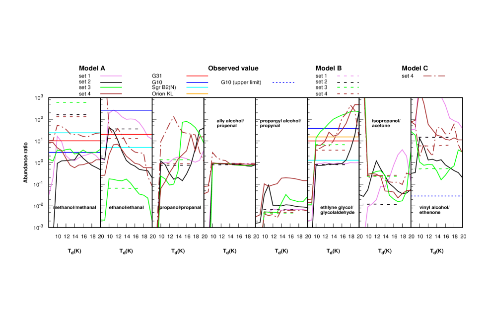
Figure 6: The obtained ratio in between six pairs of alcohol and aldehyde along with the ratio of alcohol-ketone and alcohol-ketene is shown. The observed ratio is marked in red (G31), blue (G10), cyan (Sgr B2(N)), and orange (Orion KL). Model A results are highlighted with solid curves whereas the same with Model B is represented with dashed curves and with Model C is represented with dot-dashed curves.

4.1 Physical conditions

Here, a physical condition is used, which is suitable to explain the properties of a hot core. Three models (Model A, Model B, and Model C ) are implemented to describe the chemical complexity around this region. The physical condition of our Model A is divided into three distinct phases. In the first phase (10⁵-10⁶ years), an isothermal (gas and grain temperature are kept the same) collapse of the cloud is considered from a minimum hydrogen number density (${n_{H}}_{min}$) $3\times 10^{3}$ cm^-3 to a maximum hydrogen number density (${n_{H}}_{max}$) 10⁷ cm^-3. During this phase, the visual extinction parameter ($A_{V}$) can gradually increase due to increased density. The following relation between $A_{V}$ and n_H is used to consider this situation (Lee et al., 1996; Gorai et al., 2020; Das & Chakrabarti, 2011).

$$A_{V}=max({A_{V}}_{min},(\sqrt{n_{H}/{n_{H}}_{min}}-1)/(\sqrt{{n_{H}}_{max}/{n_{H}}_{min}}-1)\times{A_{V}}_{max}).$$ (7)

It is considered that $A_{V}$ can vary from a minimum value (${A_{V}}_{min}=2$) to a maximum value (${A_{V}}_{max}=200$. In the second phase ($5\times 10^{4}$ years), the cloud remains constant at ${n_{H}}_{max}$, ${A_{V}}_{max}$. At the end of this phase, gas and dust temperature can reach up to $200$ K. The third or last phase is a post warm-up phase (period of $1.0\times 10^{5}$ years), where $n_{H}$, A_V, and temperature are kept fixed at their respective highest values.

In the case of Model B, the pre-stellar collapsing phase is considered instead of the initial isothermal collapsing phase. In this phase, the dust temperature is allowed to decrease as the collapse proceeds. Gas temperature is kept constant at $10$ K during this collapse. The other two phases are considered the same as Model A. Dust temperature of the pre-stellar collapsing phase is calculated by using the following empirical relation proposed by Hocuk et al. (2017) and used in Shimonishi et al. (2020):

$${T_{d}}^{Hoc}=[11+5.7tanh(0.61-log_{10}(A_{V}))]{\chi}_{uv}^{1/5.9},$$ (8)

where $\chi_{uv}$ is the Draine UV field strength (Draine, 1978), corresponding to $1.7G_{0}$ using the Habing field (Habing, 1968). Here, G₀ is the Far Ultraviolet radiation field in the Habing unit ($\sim 1.6\times 10^{-3}$ erg cm^-2 s^-1) integrated over the energy range $6-13.6$eV. Here, $\chi_{uv}=1$ is used.

Model C is the same as Model A. The only difference between Model A and Model C is the isothermal collapsing time scale of the first phase. In Model C, a shorter time scale ($10^{5}$ years) for the isothermal collapse is considered. It is more relevant for high mass star-forming regions. Thus, in the case of Model A, we have a density slope of $\sim 10$ cm^-3 per year, whereas it is $\sim 100$ cm^-3 per year in the collapsing phase. The warm-up and post-warm-up timescales are kept the same as in Model A.

The physical condition described here are summarized in Figure 3. The time evolution of density, temperature, and visual extinction in the three distinct phases are shown for Model A, Model B, and Model C. The left axis of Figure 3 represents the variation of temperature and visual extinction parameter in the linear scale, whereas the right axis represents the density curve in the logarithmic scale. For the better visibility, in the top panel, temperature is plotted by scaling by a factor of 2. Model A and Model B start with an isothermal collapsing phase. In this case, the dust temperature and gas temperature are kept the same. Here, a region having an initial temperature between $8-20$ K is explored to check the sensitivity of our Model A on the initial choice of the initial temperature. The temperature range for the initial phase of Model A and Model C is highlighted with the red shaded region. The visual extinction for the initial phase (isothermal collapsing phase) of Model A and C is kept constant at 2. In the case of Model B, the gas temperature of the 1^st phase is kept fixed at $10$ K, and dust temperature is estimated based on equation 8. The initial visual extinction of Model B is varied in between $0.1-10$ (corresponds to an initial dust temperature of $16-5$ K from equation 8) to check its effect on chemical evolution. The initial choice of visual extinction parameter and its estimated dust temperature of Model B are highlighted in green and yellow, respectively, in Figure 3. In the warm-up phase of Model A, Model B, and Model C, $A_{V}$ and n_H are kept constant at their highest value, and the temperature is allowed to increase up to $200$ K. It is the typical temperature of a hot core (Garrod et al., 2008). In the post-warm-up phase, both the models have identical conditions.

4.2 Modeling results

4.2.1 Abundances

In Model A, various cases starting with the initial temperature between $8-20$ K are considered. Figure 4 shows the variation of peak abundances with respect to H₂ obtained during the simulation time scale. Six pairs of aldehyde-alcohol, one pair of ketone-alcohol, and one pair of ketene-alcohol shown. Observed abundances in G10, G31, Sgr B2(N), and Orion KL are shown in solid blue, red, cyan, and orange curves, respectively. In Figure 4, the violet solid line represents the case with set 1 BEs reported in Table 7. The solid black line represents the case with set 2. A lower value of $R$ provides more mobility to the surface species keeping the same resident time on grains. It yields a dramatic change in the production of surface species. The changes in the chemical composition of interstellar ice would reflect a significant difference between the gas phase abundances of the species shown in Figure 4. The case with set 3 is represented with the solid green line in Figure 4. The set 4 case is with the solid brown curve in Figure 4. It is evident from Figure 4 that the resulting peak abundance is highly sensitive on the choice of initial temperature. More specifically, on the dust temperature. Some cases of Model A are tested with a different gas temperature than dust and did not find significant differences in the peak abundance.

It is noticed that set 1 and set 2 BEs are helpful to explain the abundances of these aldehydes and alcohols except glycolaldehyde and ethylene glycol. The set 3 BEs deviate very much from the observed value. It is mainly because of the adopted BE values of H (148 K) and H₂ (627 K). However, with the set 4 BEs, the observed abundance of ethylene glycol could be explained. It is because set 4 considered the BE of H and H₂ same as these are in set 1 and set 2 ($650$ K and $440$ K, respectively for H and H₂). The ice phase origin of these species is evident from the results obtained from Model A. The results obtained from Model A seem to be highly sensitive to the initial dust temperature, which suggests that either these species were formed during the initial cold phase or the seeds of these species were produced during the initial stage. The final gas-phase abundance of these species is highly affected by the surface species present at the beginning of the warm-up phase. The surface species at the warm-up phase are re-processed with the elevated temperature, where radicals take an active part in building the chemical complexity. Once the warm-up phase starts, the desorption of the surface species enhances and might reach their respective sublimation temperatures and populate the gas phase. With set 4 BE and Model A, it is possible to explain the observed abundances except glycolaldehyde.

The results obtained with Model B are also shown in Figure 4. All the four cases mentioned in the context of Model A are also considered with Model B. To visualize the differences between Model A and Model B, Model B cases are highlighted with the dashed curves, but with the same color codes. It is interesting to note that for Model B, significant changes of abundance for the adopted BE parameters are noticed. Like Model A, the results of Model B are not so much sensitive to the initial choice of dust temperature. The reason behind this deviation is the adopted dust temperature at the 1^st phase of Model A and Model B (see Figure 3). In Model A, the dust remains at a constant temperature for $\sim 10^{6}$ years, whereas in Model B, in between a few times $10^{3}$ years, it drops down to temperature $<10$ K. This affects the mobility of the surface species. Since it stays at $<10$ K during its first phase of evolution, Model B does not show dramatic changes between the variation of the initial dust temperature.

The orange curve of Figure 4 represents the variation of the peak abundances of these species with set 4 and Model C. It is interesting to note that with the shorter collapsing time scale (relevant for the hot core) of Model C, peak abundances of complex organic molecules are significantly enhanced. Most of the observed abundances could be explained with set 4 of Model C. The increase in the abundances of the complex organic molecule with the shorter collapsing time is not so straightforward. Many parameters are involved in it. But the shorter collapsing time leads to a much steeper slope for the density, which means that the depletion will be much faster and the complex molecules, once produced, will have a comparatively shorter time to be destroyed further. In Figure 5, the time evolution of the gas phase and ice phase abundances of aldehydes, alcohols, ketone, and ketene with respect to H₂ are shown. Only the results obtained with Model C by considering an initial gas and ice temperature of $10$ K is shown. There is some uncertainty in the observations. Additionally, the chemical model includes lots of estimated parameters (BEs, reaction pathways, reaction rates, interaction with dust, etc.) that can induce severe skepticism. Due to these reasons, it is not easy to match all the observed abundances simultaneously. In Figure 4, the peak abundance is taken beyond the isothermal collapsing phase. Figure 5, depicts that beyond the isothermal phase these peak gas-phase abundance appeared during the warm-up phase, when the temperature varies in between $\sim 100-120$ K. So our time uncertainty is relatively small ($\sim 10^{4}$ years).

A comparison between our obtained gas-phase peak abundance with the observational results is shown in Table 6. Only the results obtained with set 4 of Model C are used to show this comparison. Minimum and maximum peak abundances obtained within the initial temperature range considered for Model C and set 4 are noted in Table 6. The errors in obtained abundances are only shown for those species which are identified herein G10. The errors are calculated by taking the uncertainty in estimating the H₂ column density and the column density obtained from rotation diagram analysis. Gorai et al. (2020) obtained an average column density of $\sim 1.35\times 10^{25}$ cm^-2 . The error in estimating the column density was $\pm 1.0\times 10^{22}$ cm^-2, which mainly arose from the uncertainty of the measured flux. The error in estimating the column density of the species is taken from Table 2. For estimating the abundance errors for glycolaldehyde, only the uncertainty in predicting the H₂ column density is considered.

It is noticed that our results can successfully explain the observed abundances.

4.2.2 Molecular ratios

In Figure 6, the temperature variation of the ratio obtained between the peak abundance of six pairs of alcohol-aldehyde, one pair of alcohol-ketone, and one pair of alcohol-ketene for Model A (solid curve), Model B (dashed curve), and Model C (dot-dashed curves) are shown. The observed ratios for G31, G10, Sgr B2(N), and Orion KL are shown with red, blue, cyan, and orange solid lines, respectively. The simulated ratio between the peak abundance of alcohol and aldehyde/ketone/ketene obtained with set 4 and Model C, along with the observed abundances of these species is noted in Table 6. Table 6 depicts the observed abundances in G31, G10, Sgr B2, and Orion KL, along with our modeled abundance. Mainly the interferometric observations (wherever available) are noted to facilitate a comparative study between the chemical complexity of these hot cores. However, it is worth pointing out that all these observations are carried out with different facilities with very diverse angular and spatial resolutions. The facility used for each observations along with the H₂ column density used to derive the abundances are noted at the footnote of Table 6. Here, the band 4 archival data of G10 is only analyzed, which reports only one alcohol-aldehyde pair (ethylene glycol-glycolaldehyde pair). These two species are recognized for the first time in this source. Earlier, Rolffs et al. (2011) obtained the methanol-methanal pair. Any transitions of methanal are not identified within our spectral bands. So, a direct comparison between our obtained ratios and others could not be performed. For example, Table 6 denotes a higher methanol abundance obtained by Rolffs et al. (2011) than ours. This is because the beam size of our band 4 observation of ALMA varies between $1.39^{{}^{\prime\prime}}-2.44^{{}^{\prime\prime}}$ ($\sim 12000-21000$ AU, considering 8.6 kpc distance). In contrast, the beam size of the submillimeter Array (SMA) observation at 345 GHz of Rolffs et al. (2011) is 0.3${}^{{}^{\prime\prime}}$ ($\sim 2600$ AU, considering 8.6 kpc distance). The integrated emission map of the methanol transitions shown in Figure 10 suggests that the methanol is more compact. So as expected, with the higher spatial resolution, Rolffs et al. (2011) can trace the more inner region of the G10, and thus they obtained a higher abundance than us. Furthermore, for deriving the abundances from Rolffs et al. (2011), a hydrogen column density of $5\times 10^{24}$ cm^-2 is used. In contrast, our abundance is derived by considering $1.35\times 10^{25}$ cm^-2 (Gorai et al., 2020), which might also create significant variation. Since our chemical model does not consider the spatial variation of the abundances, explaining the observed ratio with the suitable beam size is also out of scope for this work.

The observed ratio is calculated from the observed pair from the same source (if available). It depicts that the methanol to methanal abundance ratio in these sources can vary between $2.95-23.8$, whereas our calculated methanol to methanal ratio varies between $10-53$. The observed ratio between ethanol to ethanal varies between $5-261$, whereas our model results show it ranges between $0.08-25600$. The observed ethylene glycol to glycolaldehyde ratio varies between $1.3-37$, whereas our model derives $0.019-445$. The observed ratio between the vinyl alcohol to ethenone is $0.021$, whereas our chemical model estimates $1.78-77$. In brief, the observed ratio of three alcohol-aldehyde pairs (methanal-methanol, ethanal-ethanol, glycolaldehyde-ethylene glycol) is $>$ 1 in G10, G31, Sgr B2(N), and Orion KL. Thus, in the high-mass star-forming regions, the abundances of these alcohols are generally higher than their respective aldehydes. Our estimated molecular ratios for these alcohol-aldehyde pairs are similar to the observed values in the temperature range $12-18$ K (see Figure 6). However, in the case of the vinyl alcohol to ethenone, the observed abundance ratio could not be explained. It could be because of the consideration of the upper limit of vinyl alcohol observation from the single-dish observation of Dickens et al. (2001) for deriving the molecular ratio. A little ambiguity between our obtained ratio of the dimethyl ether (DE) and methyl formate (MF) is obtained. DE/MF $<$1 is received from our observational analysis, whereas Rolffs et al. (2011) noted it $>$1 for the same source. Also, in other high mass sources, the ratio is $>$1 (4.5 for Sgr B2, 2 for G31, and 2.5 for the Orion KL). Our modeling results find that the ratio of DE with the MF can vary between $0.12-152$.

5 Conclusions

Here, our CMMC model coupled with the observational study is used to explain the abundance of some interstellar aldehydes, ketone, ketene, along with their corresponding alcohols. It is noticed that there is both observational and theoretical evidence for production of alcohols via hydrogenation of precursor aldehydes, ketones and ketenes. The following are the main highlights of this paper.

• Various aldehydes, alcohols, and a ketone are identified in G10. Among them, ethylene glycol and propanal are detected for the first time in G10, and glycolaldehyde is tentatively detected.

• The column densities and fractional abundances of the observed molecules are estimated assuming LTE conditions. The kinetic temperatures of the gas are also evaluated, which varies from 72 K to 234 K.

• The spatial distributions of the observed species are investigated, and their zeroth-order moment maps and emitting regions are provided. However, molecular emissions are not well spatially resolved or, at best, marginally resolved. Thus, we need high angular resolution data to understand their detail distributions in G10.

• Successive hydrogenation reaction can lead to the formation of alcohol starting from the aldehyde/ketone/ketene. Extensive quantum chemical calculations are carried out to yield the TS of some of these reactions. The first step of the hydrogen addition reactions has an activation barrier, whereas the second step could be considered barrier-less radical-radical reactions. Our higher-level (CCSD(T)/aug-cc-pVTZ) ice-phase calculations depict the first step of hydrogenation reaction at the carbon atom position for all the pairs (except acetone-isopropanol) is comparatively favorable than the oxygen atom position. In the acetone-isopropanol couple, an actual TS could not be obtained for the hydrogenation to the carbon atom position. However, the lower-level calculation (DFT-B3LYP/6-31+G(d,p)) in the ice-phase shows the same trend.

• BEs of these species are computed with various substrates such as H₂O, CH₃OH, and CO. For most cases, the BE of alcohols is found to be greater than that of the corresponding aldehyde/ketone/ketene. On average, the computed BEs with CH₃OH monomer is found $\sim 1.16$ times higher, and with CO monomer, it is $\sim 2.85$ times lower than that of the water monomer. These new sets of BEs would help understand the chemical complexity, where CO and CH₃OH would also efficiently cover the icy mantle. BEs of the species reported in this study for the alcohol, aldehyde, ketone, and ketenes is a little bit on the higher side ($\sim 3000$ K) with the H₂O c-tetramer configuration. Comparatively, a higher surface temperature is needed to transfer these surface species in the gas phase. Such a high temperature is usually achieved deep inside the cloud in the hot core phase. If the grain surface pathways are the only deriving route, then species with lower BE are expected to have more extended emission than the species with relatively higher BE. Since our observed beam size was large, it is not possible to spatially resolve the inner region and comment on the dependency between the BE and size of the emitting region.

• Our CMMC model with the shorter collapsing time scale ($\sim 10^{5}$ years) was able to reproduce the observed abundance and observed ratio between various species.

Appendix A emitting diameter

The emitting diameter of each transition of the observed molecules is shown in Table 8. Here, the average emitting diameter refers to the average source size. 2D Gaussian fittings of a region (area enclosing $50\%$ line peak) of the moment map image are performed. After averaging the semi-minor and semi-major axis, the emission region’s diameters are obtained.

Table 8: The emitting diameter of each transition of observed species toward G10.47+0.03.

Species	${\rm J^{{}^{\prime}}_{K_{a}^{{}^{\prime}}K_{c}^{{}^{\prime}}}}$-${\rm J^{{}^{\prime\prime}}_{K_{a}^{{}^{\prime\prime}}K_{c}^{{}^{\prime\prime}}}}$	Frequency	Eu	Emitting diameter (average)
		(GHz)	(K)	$\theta_{s}^{{}^{\prime\prime}}$
Methanol	$\rm{11_{0,11}-11_{1,11}}$ E, vt=0	154.425832∗	166.1	1.81
($\rm{CH_{3}OH}$)	$\rm{12_{0,12}-15_{1,12}}$E, vt=0	153.281282∗	193.8	1.79
	$\rm{15_{0,15}-15_{1,15}}$E, vt=0	148.111993	290.7	1.78
	$\rm{7_{-1,7}-6_{0,6}}$E, vt=1	147.943673	356.3	1.56
	$\rm{17_{-4,13}-18_{-3,16}}$E, vt=0	131.134094	450.9	1.45
	$\rm{21_{0,21}-21_{1,21}}$E, vt=0	129.720384	546.2	1.33
	8$\rm{8_{-7,1}-7_{-6,1}}$E, vt=1	153.128697	664.5	1.23
Ethylene Glycol	$\rm{8_{4,5}-7_{3,5}}$, 1-0	153.567383	25.4	1.83
(g-HOCH2CHO)	$\rm{13_{3,11}-12_{2,10}}$, 0-0	159.768239	48.8	1.85
	$\rm{13_{9,4}-12_{9,3}}$, 0-1	130.998583	83.8	1.04
	$\rm{27_{3,25}-27_{2,26}}$, 0-0	148.082465	185.5	1.04
	$\rm{28_{7,21}-28_{6,23}}$, 1-0	131.229156	223.4	1.21
	$\rm{33_{10,23}-32_{11,22}}$, 1-1	130.115657	323.0	1.60
	$\rm{39_{8,32}-39_{7,33}}$, 1-1	153.325448	414	1.27
Acetaldehyde	$\rm{8_{3,6}-7_{3,5}}$,A	154.2746864	53.7	1.49
($\rm{CH_{3}CHO}$)	$\rm{8_{3,5}-7_{3,4}}$,E	154.296489	53.7	1.53
	$\rm{8_{4,4}-7_{4,3}}$, A	154.201471	69.5	1.38
	$\rm{8_{5,4}-7_{5,3}}$, A	154.161467	89.8	1.33
	$\rm{8_{3,5}-7_{3,4}}$, A	154.173895	114.4	1.0
Propanal	$\rm{9_{7,2}-9_{6,3}}$, A	148.005042	49.6	1.18
($\rm{CH_{3}CH_{2}CHO}$)	$\rm{10_{7,3}-10_{6,4}}$, E	147.867178	54.6	1.27
	$\rm{16_{2,15}-15_{1,14}}$, E	159.932346	68.6	0.83
	$\rm{25_{3,22}-25_{2,23}}$, A	153.554511	172.7	1.87
	$\rm{27_{5,23}-27_{4,24}}$, E	154.066288	206.2	1.08
Glycolaldehyde	$\rm{15_{0,15}-14_{114}}$	153.597995	60.5	1.26
($\rm{HOCH_{2}CHO}$)	$\rm{20_{7,13}-20_{6,14}}$	153.614231	147.0	0.89
Acetone	$\rm{12_{2,11}-11_{1,10}}$, AA	130.924799	44.1	1.28
($\rm{CH_{3}COCH_{3}}$)	$\rm{11_{5,7}-10_{4,6}}$, EE	147.684364	48.4	1.83
	$\rm{13_{2,11}-12_{3,10}}$, AE	149.395864	55.8	1.56
	$\rm{14_{3,12}-13_{2,11}}$, EE	159.2476343	63.4	1.29
	$\rm{22_{4,18}-22_{3,19}}$, EE	160.118153	157.1	1.38
	$\rm{24_{6,18}-24_{5,19}}$, EE	159.415955	198.9	1.50
	$\rm{25_{10,15}-25_{9,16}}$, AE	130.708968	241.0	1.0
	$\rm{26_{10,17}-26_{9,18}}$, EE	149.190766	251.0	1.35
Methyl formate	$\rm{11_{2,10}-10_{2,9}}$, A	130.016790	40.7	1.87
($\rm{CH_{3}OCHO}$)	$\rm{11_{2,10}-10_{2,9}}$, E	130.010105	40.7	1.80
	$\rm{12_{4,9}-11_{4,8}}$, A	148.805941	56.8	1.95
	$\rm{13_{3,11}-12_{3,10}}$, A	158.704392	59.6	1.85
	$\rm{13_{7,6}-12_{7,5}}$, A	160.178942	86.2	1.82
	$\rm{13_{7,6}-12_{7,5}}$, A	160.193496	86.2	1.66
	$\rm{13_{10,4}-12_{10,3}}$, A	159.662793	120.0	1.67
	$\rm{12_{1,12}-11_{1,11}}$, A	131.377495	230.0	1.0
	$\rm{12_{4,8}-11_{4,7}}$, E	148.575217	244.1	1.69
Dimethyl ether	$\rm{6_{1,6}-5_{0,5}}$, AA	131.406552	19.9	1.91
($\rm{CH_{3}OCH_{3}}$)	$\rm{9_{0,3}-8_{1,8}}$, AE	153.055196	40.4	1.83
	$\rm{11_{1,10}-10_{2,9}}$, AE	154.456506	62.9	1.95
	$\rm{24_{4,20}-24_{3,21}}$, EE	153.385902	297.5	1.44

Note. — ^∗ optically thick

Appendix B observed spectra toward G10

The observed, fitted and LTE spectra of observed transitions are shown in Figure 7.

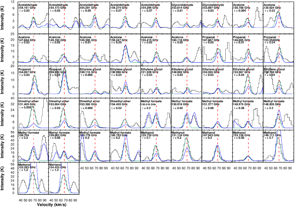
Figure 7: The observed spectra (solid black lines) along with the fitted Gaussian profile (solid green lines) and the LTE synthetic spectrum with our derived parameters (rotation temperature and column density) from rotational diagram analysis with the solid blue lines are shown. For the LTE calculation, a source size of 2${}^{{}^{\prime\prime}}$ and average FWHM obtained from the Gaussian fitting (noted in Table 1) of each species are used. The dashed red line shows the systematic velocity (V_LSR) of the source at $\sim$ 68 km s^-1. In addition, the name of the species and their respective transitions (in GHz) and optical depth of each transitions are given in each panel. Optical depth of all transitions are calculated based on the parameters assumed during LTE modeling. The last two transitions of methanol are optically thick, which are largely overproduced with the LTE consideration. The intensity of all the transitions of dimethyl ether is underproduced, possibly because our overestimated FWHM for dimethyl ether.

Appendix C Line maps

The integrated intensity distribution of all observed molecules is shown in Figures 8, 9, 10, and 11. The integrated intensity is obtained in the velocity range where the emission line is seen. It is typically obtained between 58 km/s to 78 km/s. This range slightly varies for some species. Figures 8 and 9 show the intensity distribution of the observed molecules having upper energy state $<100$ K and Figures 10 and 11 show the intensity distribution for the molecules with upper energy state $>100$ K.

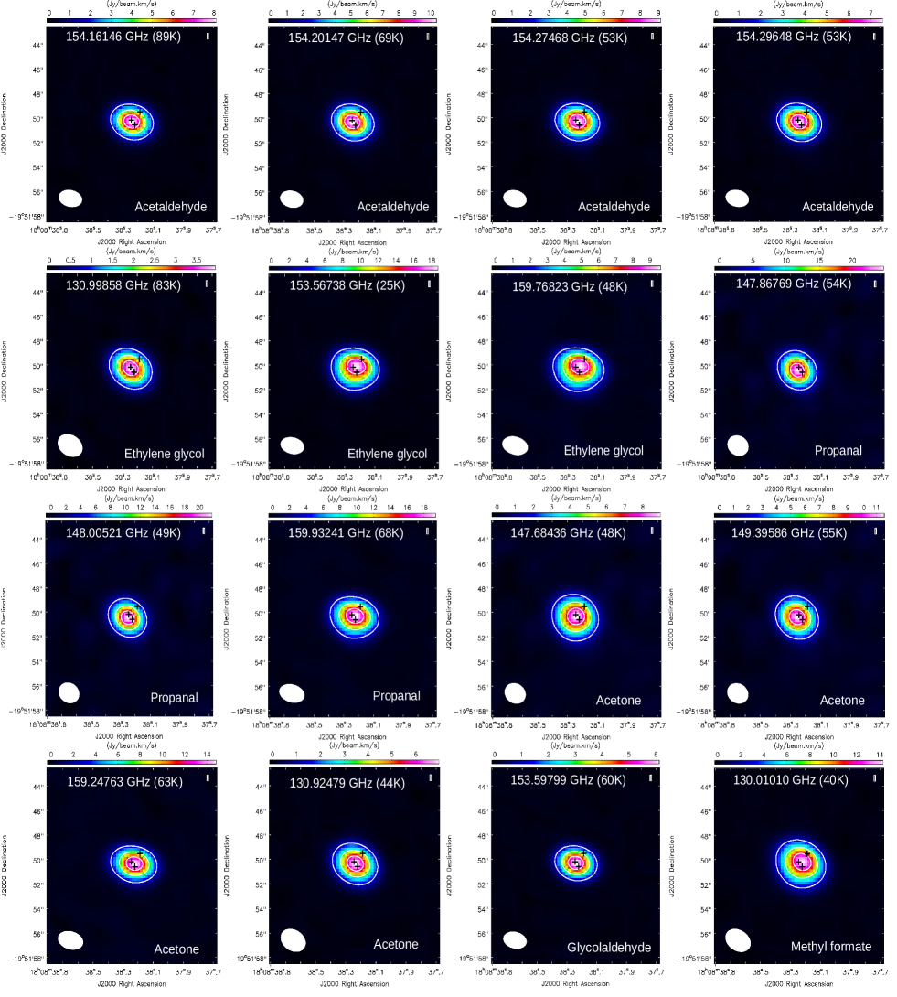
Figure 8: Integrated emission maps of observed transitions with upper energy state less than 100 K. Name of the molecules along with their respective transitions (in GHz) and upper energy state (in K) are given in each panel. The contours are shown at $20,\ 50$, and $80\%$ of maximum flux. The observed beam is shown in the lower-left corner of each figure. Three blue plus signs indicate the HII regions B1, B2, and A in the anticlockwise direction starting from the left black cross situated in the white and pink zones of continuum images (Cesaroni et al., 2010).

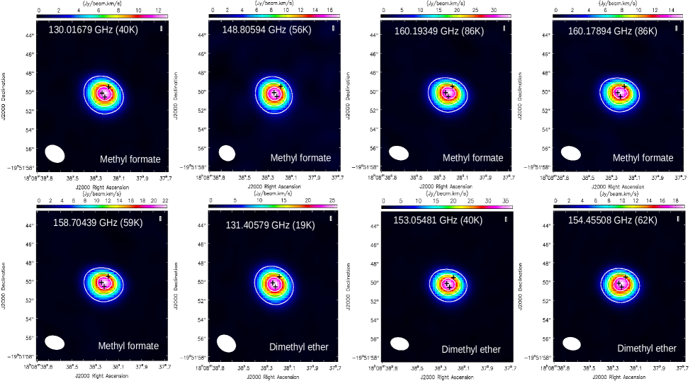
Figure 9: Same as Figure 8.

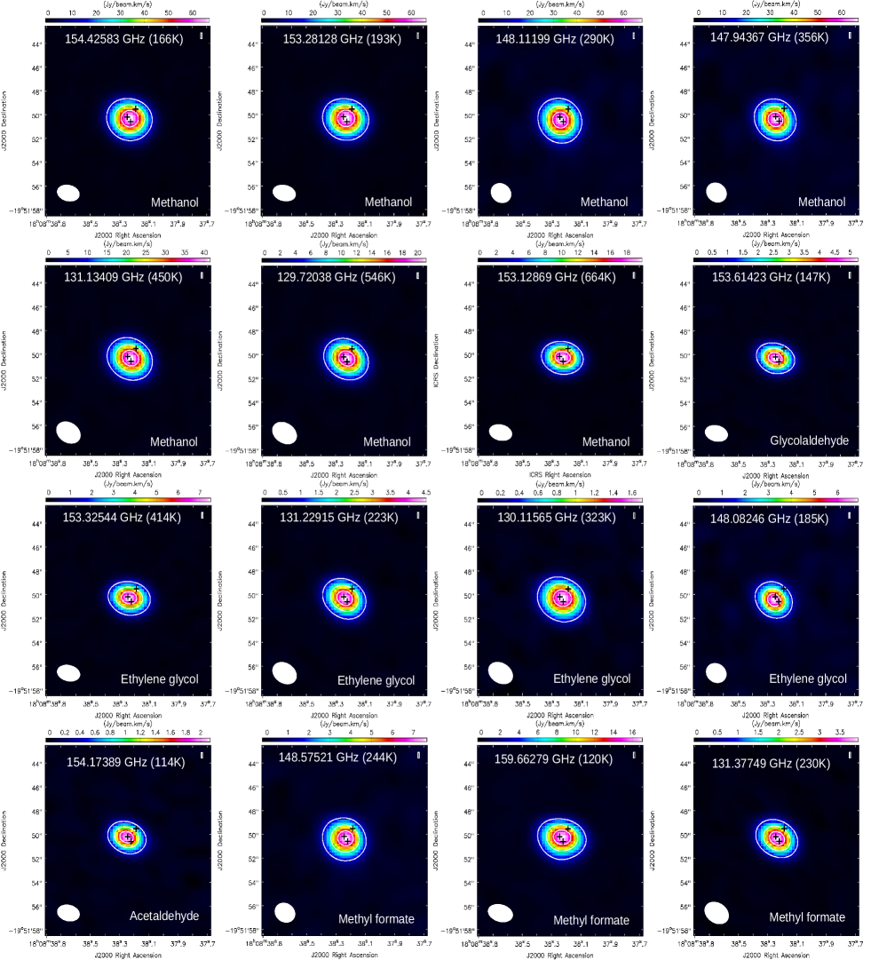
Figure 10: Integrated emission maps of observed transitions with upper energy state greater than 100 K are shown. The contours are shown at $20,\ 50$, and $80\%$ of maximum flux. The observed beam is shown in the lower-left corner of each figure. Three blue plus signs indicate the HII regions B1, B2, and A in the anti-clockwise direction starting from the left black cross situated in the white and pink zones of continuum images (Cesaroni et al., 2010).

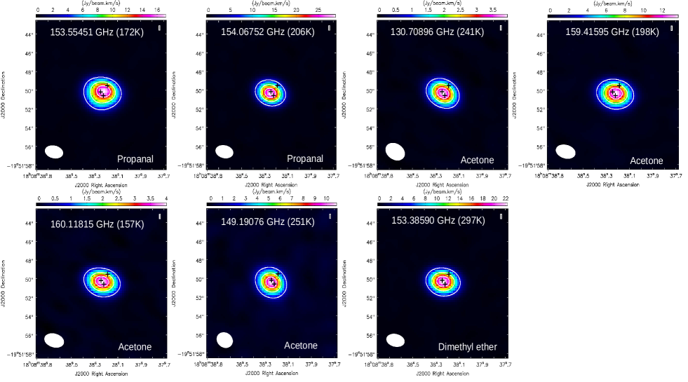
Figure 11: Same as Figure 10.

References

- Allamandola et al. (1992) Allamandola, L. J., Sandford, S. A., Tielens, A. G. G. M., & Herbst, T. M. 1992, ApJ, 399, 134
- Altwegg et al. (2017) Altwegg, K., Balsiger, H., Berthelier, J. J., et al. 2017, MNRAS, 469, S130
- Álvarez-Barcia et al. (2018) Álvarez-Barcia, S., Russ, P., Kästner, J., & Lamberts, T. 2018, MNRAS, 479, 2007
- Aragones et al. (2011) Aragones, J. L., MacDowell, L. G., & Vega, C. 2011, Journal of Physical Chemistry A, 115, 5745
- Becke (1993) Becke, A. D. 1993, The Journal of Chemical Physics, 98, 5648
- Belloche et al. (2014) Belloche, A., Garrod, R. T., Müller, H. S. P., & Menten, K. M. 2014, Science, 345, 1584
- Belloche et al. (2013) Belloche, A., Müller, H. S. P., Menten, K. M., Schilke, P., & Comito, C. 2013, A&A, 559, A47
- Beltrán et al. (2009) Beltrán, M. T., Codella, C., Viti, S., Neri, R., & Cesaroni, R. 2009, ApJ, 690, L93
- Bhat et al. (2021) Bhat, B., Gorai, P., Mondal, S. K., Chakrabarti, S. K., & Das, A. 2021, Radiative transfer modeling of the observed line profiles in G31.41+0.31, , , arXiv:2107.04979
- Bisschop et al. (2007) Bisschop, S. E., Fuchs, G. W., van Dishoeck, E. F., & Linnartz, H. 2007, A&A, 474, 1061
- Bisschop et al. (2008) Bisschop, S. E., Jørgensen, J. K., Bourke, T. L., Bottinelli, S., & van Dishoeck, E. F. 2008, A&A, 488, 959
- Biver et al. (2014) Biver, N., Bockelée-Morvan, D., Debout, V., et al. 2014, A&A, 566, L5
- Brouillet et al. (2015) Brouillet, N., Despois, D., Lu, X. H., et al. 2015, A&A, 576, A129
- Butscher et al. (2017) Butscher, T., Duvernay, F., Rimola, A., Segado-Centellas, M., & Chiavassa, T. 2017, Physical Chemistry Chemical Physics (Incorporating Faraday Transactions), 19, 2857
- Cancès et al. (1997) Cancès, E., Mennucci, B., & Tomasi, J. 1997, Journal of Chemical Physics, 107, 3032
- Carr et al. (1968) Carr, R. W., J., Gay, I. D., Glass, G. P., & Niki, H. 1968, J. Chem. Phys., 49, 846
- Cesaroni et al. (2010) Cesaroni, R., Hofner, P., Araya, E., & Kurtz, S. 2010, A&A, 509, A50
- Cesaroni et al. (1998) Cesaroni, R., Hofner, P., Walmsley, C. M., & Churchwell, E. 1998, A&A, 331, 709
- Chaabouni et al. (2012) Chaabouni, H., Bergeron, H., Baouche, S., et al. 2012, A&A, 538, A128
- Chakrabarti et al. (2006a) Chakrabarti, S. K., Das, A., Acharyya, K., & Chakrabarti, S. 2006a, A&A, 457, 167
- Chakrabarti et al. (2006b) —. 2006b, Bulletin of the Astronomical Society of India, 34, 299
- Chang et al. (2021) Chang, Q., Zheng, X.-L., Zhang, X., et al. 2021, Research in Astronomy and Astrophysics, 21, 039
- Charnley (2001) Charnley, S. 2001, The bridge between the big bang and biology, ed, Vol. 139 (F. Giovanelli, Rome: Consiglio Nazionale delle Ricerche)
- Chuang et al. (2016) Chuang, K. J., Fedoseev, G., Ioppolo, S., van Dishoeck, E. F., & Linnartz, H. 2016, MNRAS, 455, 1702
- Collins et al. (1995) Collins, P., Ferrier, R., & Berlin, W. 1995, Analytical Biochemistry, 230, 359
- Combes et al. (1987) Combes, F., Gerin, M., Wootten, A., et al. 1987, A&A, 180, L13
- Cooper et al. (2001) Cooper, G., Kimmich, N., Belisle, W., et al. 2001, Nature, 414, 879
- Córdova et al. (2005) Córdova, A., Ibrahem, I., Casas, J., et al. 2005, Chemistry (Weinheim an der Bergstrasse, Germany), 11, 4772—4784
- Coutens et al. (2018) Coutens, A., Viti, S., Rawlings, J. M. C., et al. 2018, MNRAS, 475, 2016
- Crovisier et al. (2004) Crovisier, J., Bockelée-Morvan, D., Biver, N., et al. 2004, A&A, 418, L35
- Das et al. (2008a) Das, A., Acharyya, K., Chakrabarti, S., & Chakrabarti, S. K. 2008a, A&A, 486, 209
- Das et al. (2010) Das, A., Acharyya, K., & Chakrabarti, S. K. 2010, MNRAS, 409, 789
- Das & Chakrabarti (2011) Das, A., & Chakrabarti, S. K. 2011, MNRAS, 418, 545
- Das et al. (2008b) Das, A., Chakrabarti, S. K., Acharyya, K., & Chakrabarti, S. 2008b, New A, 13, 457
- Das et al. (2019) Das, A., Gorai, P., & Chakrabarti, S. K. 2019, Astronomy & Astrophysics, 628, A73
- Das et al. (2015b) Das, A., Majumdar, L., Chakrabarti, S. K., & Sahu, D. 2015b, New A, 35, 53
- Das et al. (2015a) Das, A., Majumdar, L., Sahu, D., et al. 2015a, ApJ, 808, 21
- Das et al. (2016) Das, A., Sahu, D., Majumdar, L., & Chakrabarti, S. K. 2016, MNRAS, 455, 540
- Das et al. (2021) Das, A., Sil, M., Ghosh, R., et al. 2021, Frontiers in Astronomy and Space Sciences, 8, 78
- Das et al. (2018) Das, A., Sil, M., Gorai, P., Chakrabarti, S. i. K., & Loison, J. C. 2018, ApJS, 237, 9
- Dickens et al. (2001) Dickens, J. E., Irvine, W. M., Nummelin, A., et al. 2001, Spectrochimica Acta Part A: Molecular Spectroscopy, 57, 643
- Draine (1978) Draine, B. T. 1978, ApJS, 36, 595
- Dunning (1989) Dunning, Thom H., J. 1989, J. Chem. Phys., 90, 1007
- Endres et al. (2016) Endres, C. P., Schlemmer, S., Schilke, P., Stutzki, J., & Müller, H. S. P. 2016, Journal of Molecular Spectroscopy, 327, 95
- Etim et al. (2018) Etim, E. E., Gorai, P., Das, A., & Arunan, E. 2018, Ap&SS, 363, 6
- Favre et al. (2011) Favre, C., Despois, D., Brouillet, N., et al. 2011, HCOOCH3 as a probe of temperature and structure of Orion-KL, , , arXiv:1103.2548
- Fedoseev et al. (2017) Fedoseev, G., Chuang, K.-J., Ioppolo, S., et al. 2017, The Astrophysical Journal, 842, 52
- Fedoseev et al. (2015) Fedoseev, G., Cuppen, H. M., Ioppolo, S., Lamberts, T., & Linnartz, H. 2015, MNRAS, 448, 1288
- Fourikis et al. (1974) Fourikis, N., Sinclair, M. W., Robinson, B. J., Godfrey, P. D., & Brown, R. D. 1974, Australian Journal of Physics, 27, 425
- Frisch et al. (2013) Frisch, M. J., Trucks, G. W., Schlegel, H. B., et al. 2013, Gaussian 09 Revision D.01, , , gaussian Inc. Wallingford CT
- Fuchs et al. (2009) Fuchs, G. W., Cuppen, H. M., Ioppolo, S., et al. 2009, A&A, 505, 629
- Furuya & Persson (2018) Furuya, K., & Persson, M. V. 2018, MNRAS, 476, 4994
- Garrod & Herbst (2006) Garrod, R. T., & Herbst, E. 2006, A&A, 457, 927
- Garrod & Pauly (2011) Garrod, R. T., & Pauly, T. 2011, The Astrophysical Journal, 735, 15
- Garrod et al. (2007) Garrod, R. T., Wakelam, V., & Herbst, E. 2007, A&A, 467, 1103
- Garrod et al. (2008) Garrod, R. T., Weaver, S. L. W., & Herbst, E. 2008, The Astrophysical Journal, 682, 283
- Gibb et al. (2004) Gibb, A. G., Wyrowski, F., & Mundy, L. G. 2004, ApJ, 616, 301
- Goldsmith & Langer (1999) Goldsmith, P. F., & Langer, W. D. 1999, ApJ, 517, 209
- Gorai et al. (2020) Gorai, P., Bhat, B., Sil, M., et al. 2020, ApJ, 895, 86
- Gorai et al. (2017a) Gorai, P., Das, A., Das, A., et al. 2017a, ApJ, 836, 70
- Gorai et al. (2017b) Gorai, P., Das, A., Majumdar, L., et al. 2017b, Molecular Astrophysics, 6, 36
- Gorai et al. (2021) Gorai, P., Das, A., Shimonishi, T., et al. 2021, ApJ, 907, 108
- Gottlieb (1973) Gottlieb, C. A. 1973, in Molecules in the Galactic Environment, ed. M. A. Gordon & L. E. Snyder, 181
- Goumans (2011) Goumans, T. P. M. 2011, MNRAS, 413, 2615
- Habing (1968) Habing, H. J. 1968, Bull. Astron. Inst. Netherlands, 19, 421
- Herbst & Leung (1986) Herbst, E., & Leung, C. M. 1986, ApJ, 310, 378
- Hincelin et al. (2015) Hincelin, U., Chang, Q., & Herbst, E. 2015, A&A, 574, A24
- Hiraoka et al. (1998) Hiraoka, K., Yamashita, A., Miyagoshi, T., et al. 1998, The Astrophysical Journal, 508, 423
- Hocuk et al. (2017) Hocuk, S., Szűcs, L., Caselli, P., et al. 2017, A&A, 604, A58
- Hollis et al. (2004) Hollis, J. M., Jewell, P. R., Lovas, F. J., Remijan, A., & Møllendal, H. 2004, ApJ, 610, L21
- Hollis et al. (2002) Hollis, J. M., Lovas, F. J., Jewell, P. R., & Coudert, L. H. 2002, ApJ, 571, L59
- Hunter & Lias (1998) Hunter, E. P. L., & Lias, S. G. 1998, Journal of Physical and Chemical Reference Data, 27, 413
- Ikeda et al. (2001) Ikeda, M., Ohishi, M., Nummelin, A., et al. 2001, ApJ, 560, 792
- Käser et al. (2020) Käser, S., Unke, O. T., & Meuwly, M. 2020, The Journal of Chemical Physics, 152, 214304
- Keane et al. (2001) Keane, J. V., Tielens, A. G. G. M., Boogert, A. C. A., Schutte, W. A., & Whittet, D. C. B. 2001, A&A, 376, 254
- Lee et al. (1996) Lee, H. H., Herbst, E., Pineau des Forets, G., Roueff, E., & Le Bourlot, J. 1996, A&A, 311, 690
- Maury et al. (2014) Maury, A. J., Belloche, A., André, P., et al. 2014, A&A, 563, L2
- McElroy et al. (2013) McElroy, D., Walsh, C., Markwick, A. J., et al. 2013, A&A, 550, A36
- McGuire (2018) McGuire, B. A. 2018, ApJS, 239, 17
- McMullin et al. (2007) McMullin, J. P., Waters, B., Schiebel, D., Young, W., & Golap, K. 2007, in Astronomical Society of the Pacific Conference Series, Vol. 376, Astronomical Data Analysis Software and Systems XVI, ed. R. A. Shaw, F. Hill, & D. J. Bell, 127
- Menten et al. (1988) Menten, K. M., Walmsley, C. M., Henkel, C., & Wilson, T. L. 1988, A&A, 198, 253
- Müller et al. (2005) Müller, H. S. P., Schlöder, F., Stutzki, J., & Winnewisser, G. 2005, Journal of Molecular Structure, 742, 215
- Müller et al. (2001) Müller, H. S. P., Thorwirth, S., Roth, D. A., & Winnewisser, G. 2001, A&A, 370, L49
- Nummelin et al. (1998) Nummelin, A., Dickens, J. E., Bergman, P., et al. 1998, A&A, 337, 275
- Öberg et al. (2007) Öberg, K. I., Fuchs, G. W., Awad, Z., et al. 2007, ApJ, 662, L23
- Öberg et al. (2009) Öberg, K. I., Garrod, R. T., van Dishoeck, E. F., & Linnartz, H. 2009, A&A, 504, 891
- Olmi et al. (1996) Olmi, L., Cesaroni, R., & Walmsley, C. M. 1996, A&A, 307, 599
- Pascual-Ahuir et al. (1987) Pascual-Ahuir, J., Silla, E., Tomasi, J., & Bonaccorsi, R. 1987, Journal of Computational Chemistry, 8, 778
- Persson et al. (2018) Persson, M. V., Jørgensen, J. K., Müller, H. S. P., et al. 2018, A&A, 610, A54
- Pickett et al. (1998) Pickett, H. M., Poynter, R. L., Cohen, E. A., et al. 1998, J. Quant. Spec. Radiat. Transf., 60, 883
- Pizzarello & Weber (2004) Pizzarello, S., & Weber, A. L. 2004, Science, 303, 1151
- Pontoppidan et al. (2003) Pontoppidan, K. M., Dartois, E., van Dishoeck, E. F., Thi, W. F., & d’Hendecourt, L. 2003, A&A, 404, L17
- Qasim et al. (2019) Qasim, D., Fedoseev, G., Chuang, K. J., et al. 2019, A&A, 627, A1
- Requena-Torres et al. (2006) Requena-Torres, M. A., Martín-Pintado, J., Rodríguez-Franco, A., et al. 2006, A&A, 455, 971
- Rimola et al. (2014) Rimola, A., Taquet, V., Ugliengo, P., Balucani, N., & Ceccarelli, C. 2014, A&A, 572, A70
- Rivilla et al. (2017) Rivilla, V. M., Beltrán, M. T., Cesaroni, R., et al. 2017, A&A, 598, A59
- Rolffs et al. (2011) Rolffs, R., Schilke, P., Zhang, Q., & Zapata, L. 2011, A&A, 536, A33
- Sánchez-Monge et al. (2018) Sánchez-Monge, Á., Schilke, P., Ginsburg, A., Cesaroni, R., & Schmiedeke, A. 2018, A&A, 609, A101
- Sanna et al. (2014) Sanna, A., Reid, M. J., Menten, K. M., et al. 2014, The Astrophysical Journal, 781, 108
- Shimonishi et al. (2020) Shimonishi, T., Das, A., Sakai, N., et al. 2020, ApJ, 891, 164
- Sil et al. (2018) Sil, M., Gorai, P., Das, A., et al. 2018, ApJ, 853, 139
- Sil et al. (2017) Sil, M., Gorai, P., Das, A., Sahu, D., & Chakrabarti, S. K. 2017, European Physical Journal D, 71, 45
- Sil et al. (2021) Sil, M., Srivastav, S., Bhat, B., et al. 2021, arXiv e-prints, arXiv:2105.14569
- Snyder et al. (1969) Snyder, L. E., Buhl, D., Zuckerman, B., & Palmer, P. 1969, Phys. Rev. Lett., 22, 679
- Song & Kästner (2017) Song, L., & Kästner, J. 2017, ApJ, 850, 118
- Tercero et al. (2015) Tercero, B., Cernicharo, J., López, A., et al. 2015, A&A, 582, L1
- Tomasi et al. (2005) Tomasi, J., Mennucci, B., & Cammi, R. 2005, Chemical Reviews, 105, 2999, pMID: 16092826
- Tomasi & Persico (1994) Tomasi, J., & Persico, M. 1994, Chemical Reviews, 94, 2027
- Turner et al. (2020) Turner, A. M., Koutsogiannis, A. S., Kleimeier, N. F., et al. 2020, ApJ, 896, 88
- Turner (1977) Turner, B. E. 1977, ApJ, 213, L75
- Turner & Apponi (2001) Turner, B. E., & Apponi, A. J. 2001, ApJ, 561, L207
- Vastel et al. (2015) Vastel, C., Bottinelli, S., Caux, E., Glorian, J. M., & Boiziot, M. 2015, in SF2A-2015: Proceedings of the Annual meeting of the French Society of Astronomy and Astrophysics, 313–316
- Wakelam & Herbst (2008) Wakelam, V., & Herbst, E. 2008, ApJ, 680, 371
- Wakelam et al. (2017) Wakelam, V., Loison, J. C., Mereau, R., & Ruaud, M. 2017, Molecular Astrophysics, 6, 22
- Wakelam et al. (2010) Wakelam, V., Smith, I. W. M., Herbst, E., et al. 2010, Space Sci. Rev., 156, 13
- Watanabe & Kouchi (2002) Watanabe, N., & Kouchi, A. 2002, The Astrophysical Journal, 571, L173
- Weaver et al. (2018) Weaver, S. W., Powers, C. R., McCabe, M. N., & Zinga, S. 2018, IAU Symposium, 332, 305
- Weber (1998) Weber, A. L. 1998, Origins of Life and Evolution of the Biosphere, 28, 259
- Woods et al. (2013) Woods, P. M., Slater, B., Raza, Z., et al. 2013, ApJ, 777, 90
- Woon (2002a) Woon, D. E. 2002a, ApJ, 569, 541
- Woon (2002b) —. 2002b, ApJ, 571, L177
- Wyrowski et al. (1999) Wyrowski, F., Schilke, P., & Walmsley, C. M. 1999, A&A, 341, 882
- Zaverkin et al. (2018) Zaverkin, V., Lamberts, T., Markmeyer, M. N., & Kästner, J. 2018, A&A, 617, A25
- Zuckerman et al. (1975) Zuckerman, B., Turner, B. E., Johnson, D. R., et al. 1975, ApJ, 196, L99