Hardware-Aware Beamspace Precoding for All-Digital mmWave Massive MU-MIMO

Abstract

Massive multi-user multiple-input multiple-output (MU-MIMO) wireless systems operating at millimeter-wave (mmWave) frequencies enable simultaneous wideband data transmission to a large number of users. In order to reduce the complexity of MU precoding in all-digital basestation architectures, we propose a two-stage precoding architecture that first performs precoding using a sparse matrix in the beamspace domain, followed by an inverse fast Fourier transform that converts the result to the antenna domain. The sparse precoding matrix requires a small number of multipliers and enables regular hardware architectures, which allows the design of hardware-efficient all-digital precoders. Simulation results demonstrate that our methods approach the error-rate of conventional Wiener filter precoding with more than 2$\bm{\times}$ reduced complexity.

I Introduction

Massive multi-user (MU) multiple-input multiple-output (MIMO) systems operating at millimeter-wave (mmWave) frequencies enable simultaneous, wideband wireless transmission to a large number of user equipments (UEs) [1, 2]. While the large contiguous bandwidths available at mmWave frequencies enable high per-UE data rates, the strong atmospheric absorption necessitates MU precoding to provide sufficiently high signal-to-noise ratios (SNRs) at the UE side. Since massive MU-MIMO equips the infrastructure basestations (BSs) with a large number of antennas, fine-grained beamforming and simultaneous data transmission to multiple UEs via spatial multiplexing is possible. Hybrid analog-digital beamforming architectures for mmWave systems have been proposed in [3, 4, 5]. However, recent results in [6, 7, 8] suggest that all-digital architectures enable superior beamforming and spatial multiplexing capabilities, while achieving comparable system costs and radio-frequency (RF) power consumption by deploying low-precision data converters. In order to successfully deploy all-digital BS architectures in practice, novel hardware- and power-efficient baseband processing algorithms for channel estimation, data detection, and MU precoding are necessary.

An emerging approach towards low-complexity baseband processing algorithms and simpler hardware architectures for all-digital BSs is to exploit beamspace sparsity [9, 10, 11, 12, 13, 14, 15]. Since mmWave propagation is highly directional, the UE signals arrive at the BS from only a few incident angles [2]. By taking a spatial discrete Fourier transform (DFT) across the antenna array (e.g., a uniform linear array), the received signal is transformed from the antenna domain to the beamspace domain, which concisely reveals the underlying angular sparsity [3, 16, 17]. The sparse nature of the received beamspace signals can then be exploited in order to design low-complexity baseband algorithms and more efficient hardware architectures [9, 10, 11, 12, 14, 13, 15]. In the uplink, beamspace data detectors have been proposed in [14, 15] and beamspace channel estimators in [18, 19, 12, 20]. In the downlink, MU beamspace precoders have been proposed only recently in [21, 22, 13, 11, 23].

I-A Contributions

We propose two-stage beamspace precoding algorithms for all-digital mmWave massive MU-MIMO systems. Our algorithms rely on orthogonal matching pursuit (OMP) to compute sparse precoding matrices in the beamspace domain, which can result in lower precoding complexity than conventional, linear antenna-domain precoders that perform a dense matrix-vector product. The precoded output is then converted to the antenna domain using an inverse fast Fourier transform (IFFT). We use simulations for mmWave channels to demonstrate that our algorithms approach the bit error-rate (BER) performance of conventional, antenna-domain Wiener filter (WF) precoding, while reducing the complexity by more than 2$\times$.

I-B Notation

Boldface lowercase and uppercase letters represent vectors and matrices, respectively. For a vector $\mathbf{a}$, the $k$th entry is $a_{k}=[\mathbf{a}]_{k}$. For a matrix $\mathbf{A}$, the transpose is $\mathbf{A}^{\textnormal{T}}$ and the conjugate transpose is $\mathbf{A}^{\textnormal{H}}$; the $k$th column is $\mathbf{a}_{k}=[\mathbf{A}]_{k}$ and the $k$th row is $\underline{\mathbf{a}}_{k}=[\mathbf{A}^{\textnormal{T}}]_{k}^{\textnormal{T}}$. For an index set $\Omega$, $\mathbf{A}_{\Omega}$ refers to the submatrix of $\mathbf{A}$ with columns taken from $\Omega$. The $\ell_{2}$-norm of $\mathbf{a}$ is $\|\mathbf{a}\|$, the number of nonzero entries of $\mathbf{a}$ is denoted by $\|\mathbf{a}\|_{0}$, and the Frobenius norm of $\mathbf{A}$ is $\|\mathbf{A}\|_{F}$. The $N\times N$ identity matrix is $\mathbf{I}_{N}$ and the $N\times M$ all-zeros matrix is $\mathbf{0}_{N\times M}$. The $N\times N$ unitary DFT matrix is $\mathbf{F}_{N}$. The unit vector $\mathbf{e}_{n}$ contains a $1$ in the $n$th entry and zeros otherwise. Vectors and matrices in the beamspace domain are denoted with a bar, e.g., $\bar{}\mathbf{a}$ and $\bar{}\mathbf{A}$. The set of integers $\{1,\dots,N\}$ is $\ldbrack N\rdbrack$.

II mmWave Massive MU-MIMO Downlink

II-A Downlink Channel and System Model

We consider the mmWave massive MU-MIMO downlink, in which a BS with a $B$-antenna uniform linear array (ULA) transmits data to $U$ single-antenna For illustrative purposes only, we model wave propagation from the BS to UE $u$ with the standard plane-wave approximation [24] ${\underline{\mathbf{h}}}_{u}=\sum_{\ell=0}^{L-1}\alpha_{\ell}\underline{\mathbf{a}}(\phi_{\ell})$, where $L$ refers to the number of transmission paths between UE $u$ and the BS antenna array (including a possible LoS path), $\alpha_{l}\in\mathbb{C}$ is the complex-valued channel gain of the $\ell$th transmission path, and

$$\underline{\mathbf{a}}(\phi_{\ell})=\big{[}1,e^{j\phi_{\ell}},e^{j2\phi_{\ell}},\dots,e^{j(B-1)\phi_{\ell}}\big{]},$$ (1)

where $\phi_{\ell}$ is the spatial frequency determined by the $\ell$th path’s incident angle to the ULA. The downlink channel matrix $\mathbf{H}\in\mathbb{C}^{U\times B}$ comprises the rows ${\underline{\mathbf{h}}}_{u}$ for $u\in\ldbrack U\rdbrack$. In sec:results, we show simulation results with more realistic mmWave channel vectors that do not rely on the plane-wave approximation, generated from the mmMAGIC QuaDRiGa model [25].

We consider a block-fading frequency-flat channel, in which the channel stays constant over a block of $T$ time slots. We model the downlink input-output relation as follows:

$$\mathbf{y}=\mathbf{H}\mathbf{x}+\mathbf{n}.$$ (2)

Here, the $U$-dimensional vector $\mathbf{y}\in\mathbb{C}^{U}$ comprises the signals received at all $U$ UEs and the entries of the noise vector $\mathbf{n}\in\mathbb{C}^{B}$ are i.i.d. circularly-symmetric complex Gaussian with (known) variance $N_{0}$. To mitigate MU interference, the BS must precode the transmit symbols. To this end, a $B$-dimensional antenna-domain precoded vector $\mathbf{x}$ is formed according to

$$\mathbf{x}=\mathcal{P}(\mathbf{s},\mathbf{H},N_{0},\rho^{2}),$$ (3)

where the transmit vector $\mathbf{s}\in\mathcal{O}^{U}$ contains the $U$ data symbols to be transmitted to the UEs, $\mathcal{O}$ is the constellation set (e.g., 16-QAM), the transmit signals are assumed to be i.i.d. zero-mean and normalized so that $\operatorname{\mathbb{E}}\mathopen{}\left[|s_{u}|^{2}\right]=E_{s}$ for all $u\in\ldbrack U\rdbrack$ and $\rho^{2}$ is the average power constraint so that $\operatorname{\mathbb{E}}_{\mathbf{s}}\mathopen{}\left[\|\mathbf{x}\|^{2}\right]\leq\rho^{2}$.

II-B MSE-Optimal Linear Precoding

To minimize the precoding complexity, we focus on linear precoders for which the precoding rule in (3) is linear, i.e.,

$$\mathbf{x}=\mathcal{P}(\mathbf{s},\mathbf{H},N_{0},\rho^{2})=\mathbf{P}\mathbf{s}$$ (4)

with the precoding matrix $\mathbf{P}\in\mathbb{C}^{B\times U}$. Since multi-antenna transmission causes an array gain, each UE $u$ performs scalar equalization of the received signal $y_{u}$ with a precoding factor $\beta_{u}\in\mathbb{C}$ according to $\hat{s}_{u}=\beta_{u}y_{u}$, $u=1,\ldots,U$. As in [26], we consider pilot-based estimation of the precoding factors: In the first time slot, the BS transmits $U$ pilots with energy $E_{s}$, which are then used at each UE to estimate $\beta_{u}$.

We focus on linear precoders that minimize the UE-side mean-square error (MSE) for a common $\beta\in\mathbb{C}$ so that

MSE $$\triangleq\operatorname{\mathbb{E}}_{\mathbf{s},\mathbf{n}}\mathopen{}\left[\|\mathbf{s}-\hat{}\mathbf{s}\|^{2}\right]=\operatorname{\mathbb{E}}_{\mathbf{s},\mathbf{n}}\mathopen{}\left[\|\mathbf{s}-\beta\mathbf{y}\|^{2}\right]$$ (5)

$$=\operatorname{\mathbb{E}}_{\mathbf{s}}\mathopen{}\left[\|\mathbf{s}-\beta\mathbf{H}\mathbf{x}\|^{2}\right]+|\beta|^{2}UN_{0}$$ (6)

is minimized. The MSE-optimal linear precoder is known as the Wiener filter (WF) precoder [27], where the precoding matrix $\mathbf{P}^{\text{WF}}=\mathbf{Q}^{\text{WF}}/\beta(\mathbf{Q}^{\text{WF}})$ is given by

$$\mathbf{Q}^{\text{WF}}=\left(\mathbf{H}^{H}\mathbf{H}+\kappa^{\text{WF}}\mathbf{I}_{B}\right)^{-1}\mathbf{H}^{H}.$$ (7)

Here, $\kappa^{\text{WF}}={UN_{0}}/{\rho^{2}}$, and $\beta:\mathbb{C}^{B\times U}\to\mathbb{R}$ is a function that computes a pre-factor to satisfy the power constraint:

$$\beta(\mathbf{Q})=\textstyle\sqrt{{\operatorname{tr}\big{(}\mathbf{Q}^{H}\mathbf{Q}\big{)}E_{s}}/{\rho^{2}}}.$$ (8)

As it will become useful later, one can alternatively obtain the (unnormalized) WF precoding matrix $\mathbf{Q}^{\text{WF}}$ in (7) by solving the following unconstrained optimization problem [28]:

$$\mathbf{Q}^{\text{WF}}=\operatorname*{arg\;min}_{\mathbf{Q}\in\mathbb{C}^{B\times U}}\,\,\|\mathbf{H}\mathbf{Q}-\mathbf{I}_{U}\|_{F}^{2}+\kappa^{\text{WF}}\|\mathbf{Q}\|_{F}^{2}.$$ (9)

II-C Linear Precoding in the Beamspace Domain

In order to reduce the complexity of conventional, antenna-domain WF precoding $\mathbf{x}=\mathbf{P}^{\text{WF}}\mathbf{s}$, one can perform linear precoding in the beamspace domain [13]. The key idea is to deploy linear precoders of the following form:

$$\mathbf{x}=\mathcal{P}(\mathbf{s},{\bar{}\mathbf{H}},N_{0},\rho^{2})=\mathbf{F}_{B}^{\textnormal{H}}{\bar{}\mathbf{P}}\mathbf{s}.$$ (10)

Here, $\bar{}\mathbf{H}=\mathbf{H}\mathbf{F}_{B}$ is the beamspace representation of the mmWave MIMO channel matrix. Since the rows of $\mathbf{H}$ consist of a superposition of a few complex-valued sinusoids, e.g., as in (1), the rows of $\bar{}\mathbf{H}$ are sparse [3, 29, 30, 17] and large entries correspond to the strong transmission paths, i.e., the beams for each user. This property enables one to design beamspace precoding matrices $\bar{}\mathbf{P}$ with sparse columns, in which the nonzero entries correspond to the selected beams from the rows of $\bar{}\mathbf{H}$. If the number of beams is proportional to $U$, then we can capture the beams that carry the information of all users. We then compute the beamspace-domain precoding vector $\bar{}\mathbf{x}=\bar{}\mathbf{P}\mathbf{s}$, which requires lower complexity than eq:linearprecoding due to fewer nonzero multiplications. Finally, we convert $\bar{}\mathbf{x}$ into the antenna domain using an IFFT as in eq:linearbeamspaceprecoding.

III Sparse Beamspace Precoding Algorithms

We now propose algorithms to compute sparse precoding matrices that are suitable for beamspace precoding as in (10). We start by an OMP-based algorithm, and then propose alternative algorithms with additional structure on the sparse matrix $\bar{}\mathbf{P}$, which simplify corresponding hardware architectures.

III-A Sparse Beamspace Precoding (SBP)

In order to design SBP matrices, we modify the optimization problem in (9) to deliver sparse matrices. Our algorithms do not guarantee that the solution to a sparsity-constrained version of (9) is equal to that of the sparsity-constrained MSE minimization problem. However, our results show that our methods lead to solutions with small MSE. As a first method, we propose to solve the following optimization problem

$$\bar{}\mathbf{Q}^{\text{SBP}}=\operatorname*{arg\;min}_{\bar{}\mathbf{Q}\in\mathfrak{S}_{\text{SBP}}}\,\,\|\bar{}\mathbf{H}\bar{}\mathbf{Q}-\mathbf{I}_{U}\|_{F}^{2}+\kappa^{\text{WF}}\|\bar{}\mathbf{Q}\|_{F}^{2}.$$ (11)

where we impose a constraint that ensures each column of $\bar{}\mathbf{Q}$ to have exactly $K$ nonzero entries, i.e.,

$$\mathfrak{S}_{\text{SBP}}\triangleq\{\bar{}\mathbf{Q}\in\mathbb{C}^{B\times U}:\|\bar{}\mathbf{q}_{u}\|_{0}=K,u=1,\ldots,U\}.$$ (12)

We then normalize the matrix $\bar{}\mathbf{Q}^{\text{SBP}}$ to obtain the SBP matrix $\bar{}\mathbf{P}^{\text{SBP}}=\bar{}\mathbf{Q}^{\text{SBP}}/\beta(\bar{}\mathbf{Q}^{\text{SBP}})$, where $\beta(\bar{}\mathbf{Q}^{\text{SBP}})$ was defined in (8). It is important to realize that one can solve the problem in (11) on a per-column basis, i.e., we can solve

$$\bar{}\mathbf{q}^{\text{SBP}}_{u}=\operatorname*{arg\;min}_{\bar{}\mathbf{q}\in\mathbb{C}^{B},\|\bar{}\mathbf{q}\|_{0}=K} \|\bar{}\mathbf{H}\bar{}\mathbf{q}-\mathbf{e}_{u}\|^{2}+\kappa^{\text{WF}}\|\bar{}\mathbf{q}\|^{2}$$ (13)

for $u=1,\ldots,U$. Unfortunately, this sparse approximation problem is NP-hard [31] and thus must be solved using approximate methods. We propose to compute an approximate solution to (13) using OMP [32], as detailed next. We note that the iterative algorithms detailed below make locally optimal decisions in every iteration, without any guarantees that the final solution will be globally optimal.

Let ${\bar{}\mathbf{q}}_{u}^{(k)}\in\mathbb{C}^{k}$ be the vector computed after the $k$th OMP iteration, and ${\bar{}\mathbf{r}}_{u}^{(k)}$ the associated residual. Let $\scalerel*{\rotatebox[origin={c}]{180.0}{$\Omega$}}{\Omega}_{u}^{(k)}$ be the set of indices of the $k$ nonzero entries of $\bar{}\mathbf{q}_{u}$, and let $\Omega_{u}^{(k)}$ be the set of available indices for the new nonzero entry in the $(k+1)$th iteration. Here, $\Omega_{u}^{(k)}=\ldbrack B\rdbrack\setminus\scalerel*{\rotatebox[origin={c}]{180.0}{$\Omega$}}{\Omega}_{u}^{(k)},\forall k$. We initialize the available and already-selected indices $\Omega^{(0)}_{u}=\ldbrack B\rdbrack$, $\scalerel*{\rotatebox[origin={c}]{180.0}{$\Omega$}}{\Omega}^{(0)}_{u}=\varnothing$, and the residual $\bar{}\mathbf{r}^{(0)}_{u}=\mathbf{e}_{u}$. Then, repeat the following three steps for iterations $k=1,\ldots,K$: (i) Identify the next best beam index by correlating the residual with the columns of $\bar{}\mathbf{H}$,

$$b_{u}^{(k)}=\operatorname*{arg\;max}_{b\in\Omega_{u}^{(k-1)}}\,|\bar{}\mathbf{h}_{b}^{\textnormal{H}}\bar{}\mathbf{r}_{u}^{(k-1)}|,$$ (14)

and augment the support set, $\scalerel*{\rotatebox[origin={c}]{180.0}{$\Omega$}}{\Omega}^{(k)}_{u}=\scalerel*{\rotatebox[origin={c}]{180.0}{$\Omega$}}{\Omega}^{(k-1)}_{u}\cup\{b^{(k)}_{u}\}$. By definition, $b^{(k)}_{u}$ is unavailable for selection in subsequent iterations and we use $\Omega^{(k)}_{u}=\Omega^{(k-1)}_{u}\setminus\{b^{(k)}_{u}\}$. (ii) Update the SBP vector as for the WF precoder,

$$\bar{}\mathbf{q}_{u}^{(k)}=(\bar{}\mathbf{H}^{\textnormal{H}}_{\scalerel*{\rotatebox[origin={c}]{180.0}{$\Omega$}}{\Omega}_{u}^{(k)}}\bar{}\mathbf{H}_{\scalerel*{\rotatebox[origin={c}]{180.0}{$\Omega$}}{\Omega}_{u}^{(k)}}+\kappa^{\text{WF}}\mathbf{I}_{k})^{-1}\bar{}\mathbf{H}^{\textnormal{H}}_{\scalerel*{\rotatebox[origin={c}]{180.0}{$\Omega$}}{\Omega}_{u}^{(k)}}\mathbf{e}_{u}.$$ (15)

(iii) Update the residual, $\bar{}\mathbf{r}_{u}^{(k)}=\mathbf{e}_{u}-\bar{}\mathbf{H}_{\scalerel*{\rotatebox[origin={c}]{180.0}{$\Omega$}}{\Omega}_{u}^{(k)}}\bar{}\mathbf{q}_{u}^{(k)}$. After $K$ iterations, the entries of $\bar{}\mathbf{q}_{u}^{(K)}$ are assigned to $[\bar{}\mathbf{q}_{u}]_{b},b\in\scalerel*{\rotatebox[origin={c}]{180.0}{$\Omega$}}{\Omega}^{(K)}$, i.e., the nonzero entries of the SBP column $\bar{}\mathbf{q}_{u}$; this procedure is repeated for all columns $\bar{}\mathbf{q}_{u}$, $u\in\ldbrack U\rdbrack$, of the unnormalized SBP matrix $\bar{}\mathbf{Q}^{\text{SBP}}$. We then normalize the sparse matrix $\bar{}\mathbf{Q}^{\text{SBP}}$ to obtain the SBP matrix $\bar{}\mathbf{P}^{\text{SBP}}=\bar{}\mathbf{Q}^{\text{SBP}}/\beta(\bar{}\mathbf{Q}^{\text{SBP}})$, where the precoding factor is given by (8). The resulting SBP matrix $\bar{}\mathbf{P}^{\text{SBP}}$ contains, as desired, exactly $KU$ nonzero entries.

III-B Row-Select Sparse Beamspace Precoding (RS)

Although the above approach results in a sparse precoding matrix with $KU$ nonzero entries, the unstructured nature of the nonzero entries in $\bar{}\mathbf{P}$ prevents efficient, parallel hardware architectures that perform the sparse matrix-vector multiplication at high rates. To overcome this issue, we propose to enforce structured sparsity in the matrix $\bar{}\mathbf{P}$ such that the rows have either all ($U$) nonzero entries or all zeros, so we can only store the nonzero rows and use efficient hardware for the sparse matrix-vector multiplication. Concretely, we aim to solve the precoding problem in (11) with the constraint set

$$\mathfrak{S}_{\text{RS}}\triangleq\textstyle\Big{\{}\bar{}\mathbf{Q}\in\mathbb{C}^{B\times U}:\, \|\underline{\bar{}\mathbf{q}}_{b}\|_{0}=\begin{cases}U,\ \text{if $b$ is selected}\\ 0,\ \text{otherwise}\end{cases}\!\!\!\!\!\!,$$

$$\|\bar{}\mathbf{q}_{u}\|_{0}=K,u=1,\ldots,U\Big{\}},$$ (16)

which requires us to find $K$ nonzero rows of the unnormalized precoding matrix $\bar{}\mathbf{Q}$, each with $U$ nonzero entries. This problem resembles a multiple measurement vector (MMV) problem [33] and we use an OMP-MMV-like algorithm; we call the method Row-Select SBP, simply denoted by RS.

Let $\scalerel*{\rotatebox[origin={c}]{180.0}{$\Omega$}}{\Omega}^{(k)}$ denote the rows of $\bar{}\mathbf{Q}$ that are selected as nonzero in the first $k$ iterations, and $\Omega^{(k)}=\ldbrack B\rdbrack\setminus\scalerel*{\rotatebox[origin={c}]{180.0}{$\Omega$}}{\Omega}^{(k)}$ the remaining ones, i.e., rows available for selection in the $(k+1)$th iteration. Let $\bar{}\mathbf{Q}^{(k)}\in\mathbb{C}^{k\times U}$ denote a submatrix of the precoding matrix computed at the $k$th iteration, and $\bar{}\mathbf{R}^{(k)}$ the residual. We initialize the set of selected nonzero rows $\scalerel*{\rotatebox[origin={c}]{180.0}{$\Omega$}}{\Omega}^{(0)}=\varnothing$ and the residual $\bar{}\mathbf{R}^{(0)}=\mathbf{I}_{U}$. We repeat the following steps for iterations $k=1,\ldots,K$: (i) Identify the next best beam index,

$$\hat{b}^{(k)}=\operatorname*{arg\;max}_{b\in\Omega^{(k-1)}}\|\bar{}\mathbf{h}_{b}^{\textnormal{H}}\bar{}\mathbf{R}^{(k-1)}\|_{2},$$ (17)

and add this index to the support set $\scalerel*{\rotatebox[origin={c}]{180.0}{$\Omega$}}{\Omega}^{(k)}=\scalerel*{\rotatebox[origin={c}]{180.0}{$\Omega$}}{\Omega}^{(k-1)}\cup\{\hat{b}^{(k)}\}$. By definition, $\Omega^{(k)}=\Omega^{(k-1)}\setminus\{\hat{b}^{(k)}\}$. (ii) Update the submatrix of the precoding matrix,

$$\bar{}\mathbf{Q}^{(k)}=(\bar{}\mathbf{H}^{\textnormal{H}}_{\scalerel*{\rotatebox[origin={c}]{180.0}{$\Omega$}}{\Omega}^{(k)}}\bar{}\mathbf{H}_{\scalerel*{\rotatebox[origin={c}]{180.0}{$\Omega$}}{\Omega}^{(k)}}+\kappa^{\text{WF}}\mathbf{I}_{k})^{-1}\bar{}\mathbf{H}^{\textnormal{H}}_{\scalerel*{\rotatebox[origin={c}]{180.0}{$\Omega$}}{\Omega}^{(k)}}.$$ (18)

(iii) Update the residual, $\bar{}\mathbf{R}^{(k)}=\mathbf{I}_{U}-\bar{}\mathbf{H}_{\scalerel*{\rotatebox[origin={c}]{180.0}{$\Omega$}}{\Omega}^{(k)}}\bar{}\mathbf{Q}^{(k)}.$ After $K$ iterations, the rows of $\bar{}\mathbf{Q}^{(K)}$ deliver the nonzero rows $\underline{\bar{}\mathbf{q}}_{b},b\in\scalerel*{\rotatebox[origin={c}]{180.0}{$\Omega$}}{\Omega}^{(K)}$, of the unnormalized RS matrix $\bar{}\mathbf{Q}^{\text{RS}}$, which has exactly $KU$ nonzero entries with $\underline{\bar{}\mathbf{q}}_{b}$ containing exactly $U$ nonzeros. The RS matrix is obtained by $\bar{}\mathbf{P}^{\text{RS}}=\bar{}\mathbf{Q}^{\text{RS}}/\beta\big{(}\bar{}\mathbf{Q}^{\text{RS}}\big{)}$ with the normalization factor given by (8).

III-C Simplified One-Shot SBP and RS Algorithms

All of the above methods require $K$ iterations to construct $K$-sparse beam vectors for each UE. To further reduce the preprocessing complexity, we propose simplified methods that require only one iteration. For the counterpart of SBP, we construct the support set $\Omega_{u}$ per user $u$ by selecting $K$ beam indices that maximize the criterion in (14). For the counterpart of RS, we construct the support set of nonzero rows by selecting the $K$ beam indices maximizing (17). We call each of these methods One-Shot SBP (1S-SBP) and One-Shot RS (1S-RS).

IV Results

IV-A Simulation Setup

We simulate line-of-sight (LoS) and non-LoS (nLoS) channel conditions, both including multiple reflective paths, using the QuaDRiGa mmMAGIC UMi model[25] at a carrier frequency of 60 GHz with $\lambda/2$-spaced antennas arranged as a ULA. We generate channel matrices for a mmWave massive MIMO system with $B=128$ antennas and $U=16$ UEs. The UEs are placed randomly in a $120^{\circ}$ circular sector around the BS between a distance of 25 m and 112 m, and we assume a minimum UE separation of $1^{\circ}$. We assume UE-side power control so that the norms of the UE’s channel vectors differ by at most $6$ dB. To account for channel estimation errors in the uplink, we assume that the BS has access to a noisy version of $\mathbf{H}$ modeled as $\hat{}\mathbf{H}=\sqrt{1-\epsilon}\mathbf{H}+\sqrt{\epsilon}\mathbf{Z}$ as in [34]. Here, $\mathbf{Z}\sim\mathcal{CN}(\mathbf{0}_{U\times B},\mathbf{I}_{N})$ models the error for pilot-based channel estimation in the uplink and we set $\epsilon=0.0099$ so that the channel estimation error corresponds to operating the system at $20$ dB SNR. In our simulations, we use the beamspace channel estimation (BEACHES) algorithm from [12], 64-QAM transmission, and UE-side hard-output data detection.

We simulate the uncoded BER versus the normalized transmit power $\rho^{2}/N_{0}$ for the sparsity parameters $K=U$ and $K=2U$ using the proposed precoders from sec:algorithms. Here, we choose $K$ proportional to $U$ to capture the beams for all users, while also aiming to keep $K$ as small as possible to minimize complexity. As baseline methods, we simulate the performance of the WF precoder from sec:linprecoding and maximum ratio transmission (MRT). We also compare with the algorithms in [13], [21], and [22], referred to as local WF, QR, and greedy beam selection (GBS), respectively. Local WF [13] approximates the beamspace channel vectors by preserving the $K$-sized window of $\underline{\bar{}\mathbf{h}}_{u}$ with the highest energy and setting the remaining entries to zero. To enable a fair comparison, the precoding coefficients are selected to minimize the MSE as in eq:mse, whereas the original objective in [13] maximizes the minimum UE-side SINR. This algorithm requires the inversion and multiplication of sparse matrices, but as sparsity is not explicitly imposed, there is no guarantee on the number of zeros in the resulting precoding matrix.

Regarding QR [21] and GBS [22], these algorithms originally pick $K=U$ beams, whereas we vary $K$ for fair comparison with our algorithms. For GBS, we implement this modification by repeating the per-user beam allocation process $K/U$ times.

IV-B Complexity Analysis

We provide a complexity analysis in tbl:complexity, in which we summarize the number of real-valued multiplications required during preprocessing (calculating the precoding matrix) and precoding (applying the precoding matrix to $T$ transmit vectors), following the analysis in [28]. As in [14], we assume a complexity of $2B\log_{2}B$ for a $B$-point (I)FFT. Since RS has the same total complexity as SBP, SBP represents both methods; the same holds for 1S-SBP and 1S-RS. For local WF, $M$ stands for the average number of nonzeros in the precoding matrix based on experiments, where we assume a zero entry if the absolute value is smaller than $10^{-7}$. For the QR and GBS methods, we assume a Householder QR factorization [35]. We note that $K$ should be larger for less sparse channels, which increases the complexity of all sparsity-exploiting algorithms.

TABLE I: Complexity of various precoding methods.

Algorithm​​​	Preprocessing complexity ​​​	Precoding complexity
WF	$2U^{3}+6BU^{2}-2U(U+1)+1$	$4TBU$
MRT	0	$4TBU$
Local WF​​​	$2UB\log_{2}B+2U^{3}+6KU^{2}-2U(U+1)+1$	$4TMU\!+\!2TB\log_{2}\!B$
QR	$2UB\log_{2}\!B+4\sum_{i=1}^{U}(i-1)(1+2(U-i))$
	$+12\sum_{i\!=\!0}^{B-K-1}(B-i)\sum_{j\!=\!0}^{U-1}(B\!-\!i\!-\!j\!)(U\!-\!j)$
	$+4U^{2}+4K\sum_{i=0}^{U-1}(U-i)$	$4TKU\!+\!2TB\log_{2}\!B$
GBS	$2UB\!\log_{2}B+12\sum_{j\!=\!0}^{U-1}(K\!-\!j)(U\!-\!j)\!+\!4U^{2}$
	$+4\sum_{i=1}^{U}(i-1)(1+2(U-i))+4K\sum_{i=0}^{U-1}(U-i)\!\!\!\!$	$4TKU\!+\!2TB\log_{2}\!B$
SBP	$2UB\log_{2}B+4KB(U+2)+2UK(K+1)$
	$+2\sum_{k=1}^{K}(k^{3}+3Uk^{2}-(U+1)k+1)$	$4TKU\!+\!2TB\log_{2}\!B$
1S-SBP	$2UB\log_{2}\!B$
	$+U(4B(U+2)+2K^{3}+6UK^{2}-2(U+1)K+1)$	$4TKU\!+\!2TB\log_{2}\!B$

In fig:complexity, we show the speed-up of the algorithms compared to MRT, which we define as the ratio of the total complexity required by MRT to that of the algorithm, with respect to the number of transmissions $T$ within a channel coherence interval. For $T\to\infty$, the asymptotic speed-up of our algorithms is $\gamma\triangleq\frac{2BU}{B\log_{2}B+2UK}$. fig:complexity reveals that QR is the most complex method. For a small coherence time $T$, GBS and WF are less complex than our algorithms, but WF could be the most preferable given that it achieves the smallest MSE. Our SBP-based methods catch up with the speed of GBS as $T$ increases, and $T$ can be as large as $10^{5}$ [14] in practical mmWave systems. We see that already for $T>10^{3}$, 1S-SBP is up to 2.91$\times$ faster than MRT. SBP requires larger $T$ and smaller $K$ than 1S-SBP to outperform the baseline methods.

IV-C Bit Error-Rate Performance

fig:berplot shows the uncoded BER for the scenarios in sec:simsetup for $B=128$ BS antennas, $U=16$ users. We consider two sparsity levels $K=16$ (a,c) and $K=32$ (b, d) under LoS (a,b) and nLoS (c,d) conditions. To compare these algorithms, we consider a target BER of $2\%$. In the LoS scenario, SBP, RS, and 1S-SBP outperform local WF, GBS and MRT. QR has a similar BER performance to our algorithms, but it is not preferable as its complexity is much higher than WF as shown in sec:complexity. For $K=U$, fig:los_u shows that the SNR required by SBP to achieve the target BER is $1.5$ dB higher than WF. In fig:los_2u, the BER of all our methods approach to that of WF. Here, the one-shot variants are the most preferable as they have lower complexity than the iterative methods, while performing similarly in BER. In the nLoS scenario of fig:nlos_u, as the channel is less sparse than in the LoS case, we observe that $K=U$ is not sufficient for any of the SBP methods to perform comparably to WF. Moreover, SBP performs worse than 1S-SBP, which exemplifies a case of our iterative algorithms leading to globally suboptimal solutions. For $K=2U$, fig:nlos_2u shows that the SNRs required by SBP and RS to achieve the target BER are $1.5$ dB higher than WF. The one-shot versions do not perform well in BER even for $K=2U$. Hence, to obtain comparable BER performance to WF, our iterative SBP algorithms are preferred over the one-shot variants if the channel vectors are less sparse.

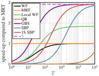
(a) $U=16,\,K=16,\gamma=2.91$

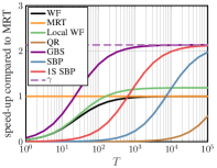
(b) $U=16,\,K=32,\gamma=2.13$

Figure 1: Speed-up compared to MRT vs the number of transmissions ($T$) evaluated by the number of real-valued multiplications for $B=128$ BS antennas, $U=16$ users, and for sparsity levels $K=U$ and $K=2U$. Our sparse beamspace precoding algorithms are up to 2.91$\times$ faster than MRT.

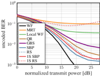
(a) LoS, $U=16,\,K=16$

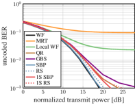
(b) LoS, $U=16,\,K=32$

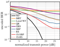
(c) nLoS, $U=16,\,K=16$

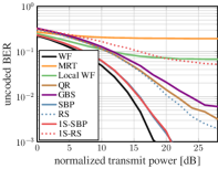
(d) nLoS, $U=16,\,K=32$

Figure 2: Bit error rate (BER) results of LoS (a,b) and nLoS (c,d) scenarios with $B=128$ BS antennas, $U=16$ users, and for sparsity levels $K=U$ and $K=2U$. The proposed sparse beamspace precoding algorithms are able to achieve a performance close to Wiener filter (WF) for sparsity level $K=2U$.

V Conclusions

We have proposed four different algorithms to perform sparse precoding in the beamspace domain. Our algorithms consist of two stages: The first stage performs sparse beamspace precoding; the second stage converts the precoded vector to the antenna domain using fast Fourier transform. Our simulation results for LoS and nLoS mmWave massive MU-MIMO channels have shown that our sparse beamspace precoding algorithms reduce the complexity by more than $2\times$ compared to traditional, antenna-domain Wiener filter precoding while delivering comparable error-rate performance. A hardware implementation of our algorithms is part of ongoing work.

References

- [1] E. G. Larsson, F. Tufvesson, O. Edfors, and T. L. Marzetta, “Massive MIMO for next generation wireless systems,” IEEE Commun. Mag., vol. 52, no. 2, pp. 186–195, Feb. 2014.
- [2] T. S. Rappaport, S. Sun, R. Mayzus, H. Zhao, Y. Azar, K. Wang, G. N. Wong, J. K. Schulz, M. Samimi, and F. Gutierrez, “Millimeter wave mobile communications for 5G cellular: It will work!” IEEE Access, vol. 1, pp. 335–349, May 2013.
- [3] A. Alkhateeb, O. El Ayach, G. Leus, and R. W. Heath Jr., “Channel estimation and hybrid precoding for millimeter wave cellular systems,” IEEE J. Sel. Topics Signal Process., vol. 8, no. 5, pp. 831–846, Oct. 2014.
- [4] Z. Gao, C. Hu, L. Dai, and Z. Wang, “Channel estimation for millimeter-wave massive MIMO with hybrid precoding over frequency-selective fading channels,” IEEE Commun. Lett., vol. 20, no. 6, pp. 1259–1262, Jun. 2016.
- [5] O. El Ayach, S. Rajagopal, S. Abu-Surra, Z. Pi, and R. W. Heath Jr., “Spatially sparse precoding in millimeter wave MIMO systems,” IEEE Trans. Wireless Commun., vol. 13, no. 3, pp. 1499–1513, Mar. 2014.
- [6] H. Yan, S. Ramesh, T. Gallagher, C. Ling, and D. Cabric, “Performance, power, and area design trade-offs in millimeter-wave transmitter beamforming architectures,” IEEE Circuits Syst. Mag., vol. 19, no. 2, pp. 33–58, May 2019.
- [7] K. Roth, H. Pirzadeh, A. L. Swindlehurst, and J. A. Nossek, “A comparison of hybrid beamforming and digital beamforming with low-resolution ADCs for multiple users and imperfect CSI,” IEEE J. Sel. Topics Signal Process., vol. 12, no. 3, pp. 484–498, Jun. 2018.
- [8] P. Skrimponis, S. Dutta, M. Mezzavilla, S. Rangan, S. H. Mirfarshbafan, C. Studer, J. Buckwalter, and M. Rodwell, “Power consumption analysis for mobile mmwave and sub-THz receivers,” in Proc. 2nd 6G Wireless Summit, Mar. 2020, pp. 1–5.
- [9] X. Gao, L. Dai, Z. Chen, Z. Wang, and Z. Zhang, “Near-optimal beam selection for beamspace mmWave massive MIMO systems,” IEEE Commun. Lett., vol. 20, no. 5, pp. 1054–1057, Mar. 2016.
- [10] C. Chen, C. Tsai, Y. Liu, W. Hung, and A. Wu, “Compressive sensing (CS) assisted low-complexity beamspace hybrid precoding for millimeter-wave MIMO systems,” IEEE Trans. Signal Process., vol. 65, no. 6, pp. 1412–1424, Dec. 2017.
- [11] A. Sayeed and J. Brady, “Beamspace MIMO for high-dimensional multiuser communication at millimeter-wave frequencies,” in Proc. IEEE Global Telecommun. Conf. (GLOBECOM), Dec. 2013, pp. 3679–3684.
- [12] S. H. Mirfarshbafan, A. Gallyas-Sanhueza, R. Ghods, and C. Studer, “Beamspace channel estimation for massive MIMO mmWave systems: Algorithm and VLSI design,” IEEE Trans. Circuits Syst. I, pp. 1–14, Sep. 2020.
- [13] M. Abdelghany, U. Madhow, and A. Tölli, “Efficient beamspace downlink precoding for mmWave massive MIMO,” in Asilomar Conf. Signals, Syst., Comput., Nov. 2019, pp. 1459–1464.
- [14] S. H. Mirfarshbafan and C. Studer, “Sparse beamspace equalization for massive MU-MIMO mmWave systems,” in Proc. IEEE Int. Conf. Acoust., Speech, Signal Process. (ICASSP), May 2020, pp. 1773–1777.
- [15] M. Mahdavi, O. Edfors, V. Öwall, and L. Liu, “Angular-domain massive MIMO detection: Algorithm, implementation, and design tradeoffs,” IEEE Trans. Circuits Syst., vol. 67, no. 6, pp. 1948–1961, Jan. 2020.
- [16] J. Mo, P. Schniter, and R. W. Heath Jr., “Channel estimation in broadband millimeter wave MIMO systems with few-bit ADCs,” IEEE Trans. Signal Process., vol. 66, no. 5, pp. 1141–1154, Mar. 2016.
- [17] J. Lee, G. Gil, and Y. H. Lee, “Channel estimation via orthogonal matching pursuit for hybrid MIMO systems in millimeter wave communications,” IEEE Trans. Commun., vol. 64, no. 6, pp. 2370–2386, Jun. 2016.
- [18] X. Gao, L. Dai, S. Han, C. I, and X. Wang, “Reliable beamspace channel estimation for millimeter-wave massive MIMO systems with lens antenna array,” IEEE Trans. Wireless Commun., vol. 16, no. 9, pp. 6010–6021, Jun. 2017.
- [19] H. He, C. Wen, S. Jin, and G. Y. Li, “Deep learning-based channel estimation for beamspace mmWave massive MIMO systems,” IEEE Commun. Lett., vol. 7, no. 5, pp. 852–855, May 2018.
- [20] L. Dai, X. Gao, S. Han, I. Chih-Lin, and X. Wang, “Beamspace channel estimation for millimeter-wave massive MIMO systems with lens antenna array,” in Int. Conf. Commun. China, Jul. 2016, pp. 1–6.
- [21] R. Pal, K. V. Srinivas, and A. K. Chaitanya, “A beam selection algorithm for millimeter-wave multi-user MIMO systems,” IEEE Commun. Lett., vol. 22, no. 4, pp. 852–855, Feb. 2018.
- [22] R. Pal, A. K. Chaitanya, and K. V. Srinivas, “Low-complexity beam selection algorithms for millimeter wave beamspace MIMO systems,” IEEE Commun. Lett., vol. 23, no. 4, pp. 768–771, Apr. 2019.
- [23] M.-F. Tang and B. Su, “Downlink precoding for multiple users in FDD massive MIMO without CSI feedback,” Springer J. Signal Process. Syst., vol. 83, no. 2, pp. 151–163, May 2016.
- [24] D. Tse and P. Viswanath, Fundamentals of Wireless Communication. Cambridge Univ. Press, 2005.
- [25] S. Jaeckel, L. Raschkowski, K. Börner, L. Thiele, F. Burkhardt, and E. Eberlein, “QuaDRiGa - Quasi Deterministic Radio Channel Generator User Manual and Documentation,” Fraunhofer Heinrich Hertz Institute, Tech. Rep. v2.0.0, 2017.
- [26] K. Li, C. Jeon, J. R. Cavallaro, and C. Studer, “Feedforward architectures for decentralized precoding in massive MU-MIMO systems,” in Proc. Asilomar Conf. Signals, Syst., Comput., Pacific Grove, CA, USA, Oct. 2018, pp. 1659–1665.
- [27] M. Joham, W. Utschick, and J. A. Nossek, “Linear transmit processing in MIMO communications systems,” IEEE Trans. Signal Process., vol. 53, no. 8, pp. 2700–2712, Aug. 2005.
- [28] O. Castañeda, S. Jacobsson, G. Durisi, T. Goldstein, and C. Studer, “Finite-alphabet MMSE equalization for all-digital massive MU-MIMO mmWave communication,” IEEE J. Sel. Areas Commun., vol. 38, no. 9, pp. 2128–2141, Jun. 2020.
- [29] P. Schniter and A. Sayeed, “Channel estimation and precoder design for millimeter-wave communications: The sparse way,” in Asilomar Conf. Signals, Syst., Comput., Nov. 2014, pp. 273–277.
- [30] A. Alkhateeb, G. Leus, and R. W. Heath Jr., “Limited feedback hybrid precoding for multi-user millimeter wave systems,” IEEE Trans. Wireless Commun., vol. 14, no. 11, pp. 6481–6494, Nov. 2015.
- [31] B. K. Natarajan, “Sparse approximate solutions to linear systems,” SIAM J Comput., vol. 24, no. 2, pp. 227–234, Apr. 1995. [Online]. Available: https://doi.org/10.1137/S0097539792240406
- [32] Y. C. Pati, R. Rezaiifar, and P. S. Krishnaprasad, “Orthogonal matching pursuit: recursive function approximation with applications to wavelet decomposition,” in Asilomar Conf. Signals, Syst., Comput., Nov. 1993, pp. 40–44 vol.1.
- [33] J. Chen and X. Huo, “Theoretical results on sparse representations of multiple-measurement vectors,” IEEE Trans. Signal Process., vol. 54, no. 12, pp. 4634–4643, Nov. 2006.
- [34] S. Jacobsson, G. Durisi, M. Coldrey, T. Goldstein, and C. Studer, “Quantized precoding for massive MU-MIMO,” IEEE Trans. Commun., vol. 65, no. 11, pp. 4670–4684, Nov. 2017.
- [35] G. H. Golub and C. F. Van Loan, Matrix Computations (3rd Ed.). USA: Johns Hopkins University Press, 1996.