Linearity conditions leading to complete positivity

Abstract

The reduced dynamics of an open quantum system $S$, interacting with its environment $E$, is not completely positive, in general. In this paper, we demonstrate that if the two following conditions are satisfied, simultaneously, then the reduced dynamics is completely positive: (1) the reduced dynamics of the system is linear, for arbitrary system-environment unitary evolution $U$; and (2) the reduced dynamics of the system is linear, for arbitrary initial state of the system $\rho_{S}$.

I Introduction

In the axiomatic approach to quantum operations, as legitimate maps describing the (reduced) dynamics of a quantum system $S$, a quantum operation $\mathcal{E}_{S}$ is defined as a linear trace-preserving completely positive map a1 . At first glance, requiring that $\mathcal{E}_{S}$ is linear seems admissible, since the unitary evolution of a closed quantum system is linear, and we may expect similar property for open quantum systems too. In addition, nonlinear evolution may lead to superluminal signaling a2 .

But, instead of being trace-preserving completely positive, one may expect that $\mathcal{E}_{S}$ must be solely a trace-preserving positive map, since the only general requirement seems to be that $\mathcal{E}_{S}$ must map density operators to density operators.

It seems that there are two major reasons, for the usual use of completely positive maps, instead of the positive ones, in quantum information theory a1 , and in the theory of open quantum systems a26 ; a27 ; a28 : First, there exists a simple operator sum representation, for each trace-preserving completely positive (CP) map $\mathcal{E}_{S}$, as

$$\mathcal{E}_{S}(\rho_{S})=\sum_{i}E_{i}\,\rho_{S}\,E_{i}^{\dagger},\ \ \ \ \ \sum_{i}E_{i}^{\dagger}E_{i}=I_{S},$$ (1)

where $E_{i}$ are linear operators and $I_{S}$ is the identity operator, on the Hilbert space of the system $\mathcal{H}_{S}$ a1 .

Second, in the theory of open quantum systems, it is common to consider the set of initial states of the system-environment as $\mathcal{S}=\{\rho_{SE}=\rho_{S}\otimes\tilde{\omega}_{E}\}$, where $\rho_{S}$ is an arbitrary state (density operator) on $\mathcal{H}_{S}$ and $\tilde{\omega}_{E}$ is a fixed state on the Hilbert space of the environment $\mathcal{H}_{E}$ a26 ; a27 ; a28 . Then, for such an initial set $\mathcal{S}$, it is famous that the reduced dynamics of the system is CP, for arbitrary system-environment unitary evolution $U$ a1 .

The main question of this paper is to investigate whether it is possible to result the CP-ness of the reduced dynamics, from its positivity, or even from the less restrictive condition of its linearity.

Unlike the reduced dynamics, for which, in general, its positivity is not equivalent to its CP-ness, there exists an important map for which it is so. This important map is the inverse of the partial trace over the environment, and is called the assignment map a23 ; a24 . It can be shown that if there exists a positive assignment map, then there exists a CP one too, which results in the CP-ness of the reduced dynamics a25 .

As we will see, in Sec. IV, only requiring that the reduced dynamics is linear, for arbitrary unitary evolution of the system-environment $U$ and arbitrary initial state of the system $\rho_{S}$, results in the positivity of the assignment map, and so the CP-ness of the reduced dynamics.

The paper is organized as follows. In the next section, we review some introductory points, on the reduced dynamics of an open quantum system. The assignment map, and its role in representing the reduced dynamics as a linear map, is introduced in Sec. III. Our main results are given in Sec. IV, and the paper is ended in Sec. V, with a summary of our results.

II Reduced dynamics of an open system

Let us denote the set of all linear operators on $\mathcal{H}_{S}$ as $\mathcal{L}_{S}$, and the set of all density operators on $\mathcal{H}_{S}$ as $\mathcal{D}_{S}$. Now, by a Hermitian map, we mean a linear trace-preserving map on $\mathcal{L}_{S}$, which maps each Hermitian operator to a Hermitian operator. A Hermitian map is called positive, if it maps each density operator, in $\mathcal{D}_{S}$, to a density operator. Both, Hermitian maps and positive ones, have operator sum representations as

$$\Phi_{S}(\rho_{S})=\sum_{i}e_{i}\,\tilde{E_{i}}\,\rho_{S}\,\tilde{E_{i}}^{\dagger},\quad\sum_{i}e_{i}\,\tilde{E_{i}}^{\dagger}\tilde{E_{i}}=I_{S},$$ (2)

where $\tilde{E_{i}}$ are linear operators on $\mathcal{H}_{S}$, and $e_{i}$ are real coefficients a3 ; a4 ; a5 . When all of the coefficients $e_{i}$ in Eq. (2) are positive, we can define $E_{i}=\sqrt{e_{i}}\,\tilde{E_{i}}$, and Eq. (2) can be rewritten as Eq. (1). Then, the map is called CP. It is also worth noting that the CP-ness of the map $\mathcal{E}_{S}$, in Eq. (1), is equivalent to the positivity of the map $\mathrm{id}_{W}\otimes\mathcal{E}_{S}$, where the witness $W$ is an arbitrary (finite dimensional) quantum system, distinct from the system $S$ (and the environment $E$), and $\mathrm{id}_{W}$ is the identity map on $\mathcal{L}_{W}$ a1 . ($\mathcal{L}_{W}$ is the set of all linear operators on the Hilbert space of the witness $\mathcal{H}_{W}$.)

For the open quantum system $S$, interacting with its environment $E$, we can consider the whole system-environment as a closed quantum system, which evolves unitarily as

$$\rho_{SE}^{\prime}=\mathrm{Ad}_{U}(\rho_{SE})\equiv U\rho_{SE}U^{\dagger},$$ (3)

where $U$ is a unitary operator, on $\mathcal{H}_{S}\otimes\mathcal{H}_{E}$. In addition, $\rho_{SE}$ and $\rho_{SE}^{\prime}$ are initial and final states of the system-environment, respectively. So, the reduced dynamics of the system is given by

$$\rho_{S}^{\prime}=\mathrm{Tr}_{E}(\rho_{SE}^{\prime})=\mathrm{Tr}_{E}\circ\mathrm{Ad}_{U}(\rho_{SE}).$$ (4)

In general, the reduced dynamics of the system $S$ cannot be represented by a map a11 ; a5 , i.e., $\rho_{S}^{\prime}$ cannot be given as a function of the initial state of the system $\rho_{S}=\mathrm{Tr}_{E}(\rho_{SE})$, in general. Even if the reduced dynamics of the system can be given by a map, this map is not linear, in general a12 ; a13 . And, even if it is linear, it is not (completely) positive, in general, but it is Hermitian a14 . The CP-ness of the reduced dynamics has been proven, only for some restricted sets $\mathcal{S}=\{\rho_{SE}\}$, of initial states of the system-environment a15 ; a16 ; a17 ; a18 ; a19 ; a20 ; a21 .

In the experimentally relevant cases, one usually deals with the factorized initial states of the system-environment, i.e., the set of initial states of the system-environment, at time $t=0$, is as $\mathcal{S}=\{\rho_{S}\otimes\tilde{\omega}_{E}\}$, where $\rho_{S}$ is an arbitrary state of the system, while $\tilde{\omega}_{E}$ is a fixed state of the environment a26 ; a27 ; a28 . So, the reduced dynamics is CP, as stated in the Introduction. But, even in such cases, one may encounter non-CP reduced dynamics, simply by changing the initial time from $t=0$, as illustrated in the following example.

Consider the case that the reduced dynamics is given by a master equation, which is similar to the Gorini-Kossakowski-Sudarshan-Lindblad one 40b ; 41b , but with a time-dependent generator $\mathcal{K}_{S}(t)$, as

$$\frac{d\sigma_{S}}{dt}=\mathcal{K}_{S}(t)[\sigma_{S}]$$ (5)

$$=-\frac{i}{\hbar}[H(t),\sigma_{S}]$$

$$\qquad+\sum_{j}\gamma_{j}(t)\left[A_{j}(t)\sigma_{S}A_{j}^{\dagger}(t)-\frac{1}{2}\{A_{j}^{\dagger}(t)A_{j}(t),\sigma_{S}\}\right],$$

where $\sigma_{S}=\sigma_{S}(t)\in\mathcal{D}_{S}$ is the reduced state of the system $S$, at time $t$. In addition, the (Hermitian) Hamiltonian operator $H(t)\in\mathcal{L}_{S}$, the Lindblad operators $A_{j}(t)\in\mathcal{L}_{S}$, and the real rates $\gamma_{j}(t)$ are all time-dependent, in general 42b . Now, if all $\gamma_{j}(t)$ are positive, for all $t\geq 0$, then the reduced dynamics is CP-divisible 42b :

$$\mathcal{E}_{S}(t_{2},0)=\mathcal{E}_{S}(t_{2},t_{1})\circ\mathcal{E}_{S}(t_{1},0),$$ (6)

where $t_{2}>t_{1}>0$, and $\mathcal{E}_{S}(t,s)$ is a CP map, which maps $\sigma_{S}(s)$ to $\sigma_{S}(t)$. But, if, in the canonical form of the generator $\mathcal{K}_{S}(t)$ 43b , all $\gamma_{j}(t)$ are positive, only during the time interval $[0,t_{1}]$, then, we have

$$\mathcal{E}_{S}(t_{2},0)=\Phi_{S}(t_{2},t_{1})\circ\mathcal{E}_{S}(t_{1},0),$$ (7)

where, though $\mathcal{E}_{S}(t_{1},0)$ and $\mathcal{E}_{S}(t_{2},0)$ are CP, but $\Phi_{S}(t_{2},t_{1})$, i.e., the Hermitian map which maps $\sigma_{S}(t_{1})$ to $\sigma_{S}(t_{2})$, is non-CP, in general. So, changing the initial time, from $t=0$ to $t=t_{1}$, results that the reduced dynamics of the system is given by the non-CP map $\Phi_{S}(t,t_{1})$, for $t>t_{1}$.

In addition to simplicity and experimental relevance, which were mentioned above and in the Introduction, one can give a rather general discussion, leading to the CP-ness of the reduced dynamics: always, in addition to the system under study $S$, one can consider another quantum system, the witness $W$, which does not interact with $S$, and, during the evolution of $S$, it does not evolve. Now, assuming that the evolution of the witness-system is given by a local map $\mathrm{id}_{W}\otimes\mathcal{E}_{S}$, results in the CP-ness of $\mathcal{E}_{S}$. Note that the initial state of the witness-system $\rho_{WS}$ can be entangled. Now, the CP-ness of $\mathcal{E}_{S}$, and so the positivity of the $\mathrm{id}_{W}\otimes\mathcal{E}_{S}$, is necessary to ensure that the final state $\rho^{\prime}_{WS}=\mathrm{id}_{W}\otimes\mathcal{E}_{S}(\rho_{WS})$ is a valid density operator a1 . However, one can find situations in which, though the dynamics of the witness-system is local (and the reduced state of the witness does not change, during the evolution), it cannot be written as $\mathrm{id}_{W}\otimes\mathcal{E}_{S}$ (see, e.g. a9aa ). So, the reduced dynamics of the system $S$ can be non-CP, in general, as we have seen for $\Phi_{S}(t,t_{1})$, in the previous paragraph.

At the end of this section, we mention that the utilization of the completely positive maps, for describing the reduced dynamics of the system $S$, can be extended, at least, through the two following ways. First, consider the case that the set of initial states of the system-environment is given by $\mathcal{S}=\{\rho_{SE}=\sum_{\alpha}\tilde{w}_{\alpha}Q_{\alpha}\otimes\tilde{\sigma}_{\alpha}\}$, where the linear operators $Q_{\alpha}\in\mathcal{L}_{S}$ vary, by changing $\rho_{SE}$, but $\tilde{\sigma}_{\alpha}$ are fixed density operators on $\mathcal{H}_{E}$, and the (positive) weights $\tilde{w}_{\alpha}$ are also fixed. Then, the reduced dynamics of the system $S$, in Eq. (4), for arbitrary system-environment unitary evolution $U$, is given by

$$\rho_{S}^{\prime}=\sum_{\alpha}\tilde{w}_{\alpha}\mathcal{E}_{S}^{(\alpha)}(Q_{\alpha}),$$ (8)

where $\mathcal{E}_{S}^{(\alpha)}$ is a CP map, depending on $U$ and $\tilde{\sigma}_{\alpha}$ bb1 . In other words, in this case, the reduced dynamics is given by a set of CP maps $\{\mathcal{E}_{S}^{(\alpha)}\}$, instead of only one CP map.

Second, consider the case that set of initial states of the system-environment is given by $\mathcal{S}=\{\rho_{SE}=\mathcal{E}_{S}\otimes\mathrm{id}_{E}(\tilde{\omega}_{SE})\}$, where $\tilde{\omega}_{SE}$ is a fixed state on $\mathcal{H}_{S}\otimes\mathcal{H}_{E}$, $\mathcal{E}_{S}$ is an arbitrary CP map on $\mathcal{L}_{S}$, and $\mathrm{id}_{E}$ is the identity map on $\mathcal{L}_{E}$, the set of all linear operators on $\mathcal{H}_{E}$. Splitting a quantum experiment into the three steps of preparation, evolution and measurement, choosing the set $\mathcal{S}$ as above means that we can only manipulate the system $S$, through the CP maps $\mathcal{E}_{S}$, during the preparation step. Now, it can be shown that, for arbitrary system-environment unitary evolution $U$, the final state of the system $\rho_{S}^{\prime}$, in Eq. (4), can be written as a completely positive map on (the Choi matrix representation a6 ; a7 of) $\mathcal{E}_{S}$ bb15 ; bb2 . In other words, in this case, even if $\rho_{S}^{\prime}$ cannot be given as a completely positive map on the initial state of the system $\rho_{S}$, but it can be given by a completely positive map, on the preparation map $\mathcal{E}_{S}$.

III Assignment map

Consider the set $\mathcal{S}=\{\rho_{SE}\}$ of initial states of the system-environment. The set $\mathcal{S}$ includes all initial $\rho_{SE}$ which are prepared (chosen), through the preparation step of the experiment. Obviously, in general, $\mathcal{S}$ is a subset of $\mathcal{D}$, the set of all density operators on $\mathcal{H}_{S}\otimes\mathcal{H}_{E}$.

The set of initial states of the system is given by $\mathcal{S}_{S}=\mathrm{Tr}_{E}\mathcal{S}$. Assuming that the system $S$ is finite dimensional, of dimension $d_{S}$, only a finite number $m$ of the members of $\mathcal{S}_{S}$, where the integer $m$ is $0<m\leq{(d_{S})}^{2}$, are linearly independent. Let us denote this linearly independent set as $\mathcal{S}^{\prime}_{S}=\{\rho_{S}^{(1)},\rho_{S}^{(2)},\ldots\ ,\rho_{S}^{(m)}\}$. Therefore, any $\rho_{S}\in\mathcal{S}_{S}$ can be expanded as

$$\rho_{S}=\sum_{i=1}^{m}a_{i}\rho_{S}^{(i)},$$ (9)

where $a_{i}$ are real coefficients. Note that $\rho_{S}$ is a Hermitian operator. So, $\sum(a_{i}-a_{i}^{*})\rho_{S}^{(i)}=0$. Now, since all $\rho_{S}^{(i)}\in\mathcal{S}_{S}^{\prime}$ are linearly independent, all $a_{i}$ must be real.

In general, there may be more than one state in $\mathcal{S}$ such that tracing over the environment gives $\rho_{S}^{(i)}$. However, we choose only one of them and denote it as $\rho_{SE}^{(i)}$. Linear independence of $\rho_{S}^{(i)}\in\mathcal{S}^{\prime}_{S}$ results in linear independence of $\rho_{SE}^{(i)}$. We denote this linearly independent set as $\mathcal{S}^{\prime}=\{\rho_{SE}^{(1)},\rho_{SE}^{(2)},\ldots\ ,\rho_{SE}^{(m)}\}$ b1 . So, each $\rho_{SE}\in\mathcal{S}$, for which $\rho_{S}=\mathrm{Tr}_{E}(\rho_{SE})$ is expanded in Eq. (9), can be written as

$$\rho_{SE}=\sum_{i=1}^{m}a_{i}\rho_{SE}^{(i)}+Y(\rho_{SE}),$$ (10)

where $a_{i}$ are the same as those in Eq. (9), and $Y$ is a Hermitian operator, on $\mathcal{H}_{S}\otimes\mathcal{H}_{E}$, such that $\mathrm{Tr}_{E}(Y)=0$. In other words, Eq. (9) results that $\rho_{SE}$ and $\sum a_{i}\rho_{SE}^{(i)}$ can differ with each other up to a Hermitian operator $Y$, for which $\mathrm{Tr}_{E}(Y)=0$. In general, $Y$ is a function of $\rho_{SE}$. This dependence is explicitly given in Eq. (10), by writing it as $Y(\rho_{SE})$.

The subspaces $\mathcal{V}$ and $\mathcal{V}_{S}$ are defined as a5

$$\mathcal{V}=\mathrm{Span}_{\mathbb{C}}\ \mathcal{S},$$ (11)

and

$$\mathcal{V}_{S}=\mathrm{Tr}_{E}\mathcal{V}=\mathrm{Span}_{\mathbb{C}}\ \mathcal{S}_{S}=\mathrm{Span}_{\mathbb{C}}\ \mathcal{S}_{S}^{\prime}.$$ (12)

Therefore, each $X\in\mathcal{V}$ can be written as $X=\sum_{l}c_{l}\,\tau_{SE}^{(l)}$, where $\tau_{SE}^{(l)}\in\mathcal{S}$, and $c_{l}$ are complex coefficients. Using Eq. (10), we can expand each $\tau_{SE}^{(l)}$ as $\tau_{SE}^{(l)}=\sum_{i}a_{li}\rho_{SE}^{(i)}+Y^{(l)}$. So,

$$X=\sum_{i=1}^{m}\left(\sum_{l}a_{li}c_{l}\right)\rho_{SE}^{(i)}+\sum_{l}c_{l}\,Y^{(l)}$$ (13)

$$=\sum_{i=1}^{m}d_{i}\rho_{SE}^{(i)}+Y(X),$$

where $d_{i}=\sum_{l}a_{li}c_{l}$ are complex coefficients, and the linear operator $Y(X)=\sum_{l}c_{l}\,Y^{(l)}$ is such that $\mathrm{Tr}_{E}(Y(X))=0$. Consequently, for each $x\in\mathcal{V}_{S}$, we have

$$x=\mathrm{Tr}_{E}(X)=\sum_{i=1}^{m}d_{i}\rho_{S}^{(i)},$$ (14)

where the coefficients $d_{i}$ are the same as those in Eq. (13). In Fig. 1, the sets $\mathcal{S}_{S}$ and $\mathcal{D}_{S}$, the subspace $\mathcal{V}_{S}$, and the vector space $\mathcal{L}_{S}$ are given, in a Venn diagram.

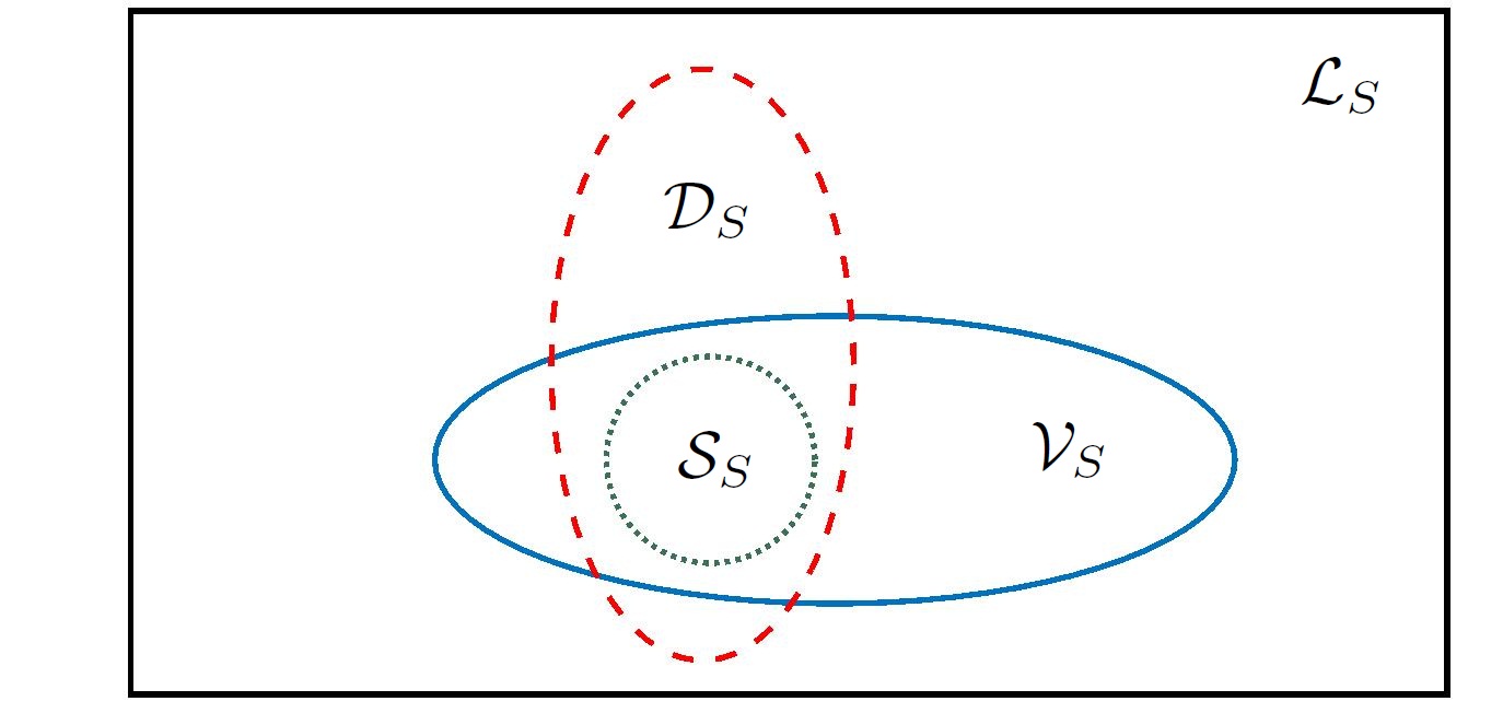
Figure 1: The set $\mathcal{S}_{S}=\mathrm{Tr}_{E}\mathcal{S}$ (green dotted circle) is the set of initial states of the system $S$. The set $\mathcal{D}_{S}$ (red dashed ellipse) is the set of all states (density operators) on $\mathcal{H}_{S}$. Obviously, $\mathcal{S}_{S}\subseteq\mathcal{D}_{S}$. The subspace $\mathcal{V}_{S}$ (blue solid ellipse) is defined in Eq. (12), and so, $\mathcal{S}_{S}\subset\mathcal{V}_{S}$. Finally, $\mathcal{L}_{S}$ (black solid rectangle) is the set of all linear operators on $\mathcal{H}_{S}$. So, $\mathcal{D}_{S}\subset\mathcal{L}_{S}$ and $\mathcal{V}_{S}\subseteq\mathcal{L}_{S}$. When $\mathcal{S}_{S}=\mathcal{D}_{S}$, then $\mathcal{V}_{S}=\mathcal{L}_{S}$.

Now, we can define the linear trace-preserving assignment map $\Lambda_{S}$, as follows: first, we define $\Lambda_{S}(\rho_{S}^{(i)})=\rho_{SE}^{(i)}$. Then, we extend the definition of $\Lambda_{S}$, to the whole $\mathcal{V}_{S}$, as a linear map. So, for any $x\in\mathcal{V}_{S}$, in Eq. (14), we have

$$\Lambda_{S}(x)=\sum_{i=1}^{m}d_{i}\Lambda_{S}(\rho_{S}^{(i)})=\sum_{i=1}^{m}d_{i}\rho_{SE}^{(i)}.$$ (15)

The assignment map $\Lambda_{S}$ maps $\mathcal{V}_{S}$ to (a subspace of) $\mathcal{V}$, and is Hermitian, by construction. (When $x$ is a Hermitian operator, all $d_{i}$, in Eq. (14), are real. So, $\Lambda_{S}(x)$ is also a Hermitian operator.) Comparing Eqs. (13) and (15) shows that $\Lambda_{S}$ does not necessarily map $x$ to $X$, unless $Y(X)=0$. In addition, note that the assignment map $\Lambda_{S}$, in Eq. (15), is defined on the subspace $\mathcal{V}_{S}$. This definition can be extended, to the whole $\mathcal{L}_{S}$, simply, i.e., one can find a Hermitian map $\Lambda_{S}^{\prime}$, on the whole $\mathcal{L}_{S}$, such that, for each $x\in\mathcal{V}_{S}$, it acts as $\Lambda_{S}$ (a25, ). But, only for each $x\in\mathcal{V}_{S}$, not necessarily for arbitrary $f\in\mathcal{L}_{S}$, we have $\mathrm{Tr}_{E}\circ\Lambda_{S}^{\prime}(x)=\mathrm{Tr}_{E}\circ\Lambda_{S}(x)=x$. In other words, the extension $\Lambda_{S}^{\prime}$ of the assignment map $\Lambda_{S}$ is self-consistent only on $\mathcal{V}_{S}$, not necessarily on the whole $\mathcal{L}_{S}$.

Now, using Eqs. (4), (9), (10) and (15), the reduced dynamics of the system, for each $\rho_{SE}\in\mathcal{V}$, is given by

$$\rho_{S}^{\prime}=\mathrm{Tr}_{E}\circ\mathrm{Ad}_{U}(\rho_{SE})$$ (16)

$$=\sum_{i=1}^{m}a_{i}\mathrm{Tr}_{E}\circ\mathrm{Ad}_{U}(\rho_{SE}^{(i)})+\mathrm{Tr}_{E}\circ\mathrm{Ad}_{U}(Y)$$

$$\qquad=\mathrm{Tr}_{E}\circ\mathrm{Ad}_{U}\circ\Lambda_{S}(\rho_{S})+\mathrm{Tr}_{E}\circ\mathrm{Ad}_{U}(Y)$$

$$=\Phi_{S}(\rho_{S})+\mathrm{Tr}_{E}\circ\mathrm{Ad}_{U}(Y),$$

where $\Phi_{S}\equiv\mathrm{Tr}_{E}\circ\mathrm{Ad}_{U}\circ\Lambda_{S}$. The map $\Phi_{S}$ is a (linear) Hermitian map on $\mathcal{V}_{S}$, since $\mathrm{Tr}_{E}$ and $\mathrm{Ad}_{U}$ are CP a1 , and the assignment map $\Lambda_{S}$ is Hermitian on $\mathcal{V}_{S}$, as we have seen in Eq. (15). When $\mathrm{Tr}_{E}\circ\mathrm{Ad}_{U}(Y)=0$, the subspace $\mathcal{V}$ is called $U$-consistent a5 . The reduced dynamics of the system, for each $\rho_{SE}\in\mathcal{V}$, is given by the linear Hermitian trace-preserving map $\Phi_{S}$, if and only if $\mathcal{V}$ is $U$-consistent a22 ; a5 . In Fig. 2, we represent when the Hermitian map $\Phi_{S}$ gives the reduced dynamics of the system, in a commutative diagram. It is also worth noting that, in the theory of open quantum systems, one usually approximates the reduced dynamics as a linear map, utilizing some simplifying assumptions (about $\mathcal{V}$) a26 ; a27 ; a28 ; 28a .

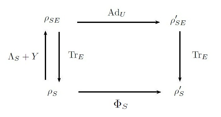
Figure 2: The state $\rho_{SE}$ is the initial state of the whole system-environment. The final state of the system-environment $\rho_{SE}^{\prime}$ is given in Eq. (3). Tracing over the environment $E$, gives the initial state of the system $\rho_{S}=\mathrm{Tr}_{E}(\rho_{SE})$, and its final state $\rho_{S}^{\prime}=\mathrm{Tr}_{E}(\rho_{SE}^{\prime})$. According to Eqs. (9), (10) and (15), $\Lambda_{S}(\rho_{S})+Y$ gives $\rho_{SE}$. The map $\Phi_{S}$ is defined as $\Phi_{S}=\mathrm{Tr}_{E}\circ\mathrm{Ad}_{U}\circ\Lambda_{S}$. According to Eq. (16), $\Phi_{S}$ gives $\rho_{S}^{\prime}$, if the $U$-consistency condition $\mathrm{Tr}_{E}\circ\mathrm{Ad}_{U}(Y)=0$ is satisfied. Then, rounding the diagram clockwise, from $\rho_{S}$ to $\rho_{S}^{\prime}$, is equivalent to rounding it counterclockwise, through the Hermitian map $\Phi_{S}$.

CP-ness of $\mathrm{Tr}_{E}$ and $\mathrm{Ad}_{U}$ results that only the assignment map $\Lambda_{S}$ determines whether $\Phi_{S}$ is CP or not. If $\Lambda_{S}$ is Hermitian, then $\Phi_{S}$ can be either Hermitian, positive or CP. But, when the extension $\Lambda_{S}^{\prime}$ of the assignment map $\Lambda_{S}$ is positive, then $\Phi_{S}$ is necessarily CP a25 .

We end this section, with the following point. Assuming unitary dynamics for the whole system-environment, the (non)linearity of the reduced dynamics is only a consequence of $U$-(in)consistency of the subspace $\mathcal{V}$. In other words, it is only a consequence of how we choose (construct) the initial set $\mathcal{S}$, and there is no fundamental reasoning behind it a22 . In addition, as discussed in Ref. a22 , non-linearity of the reduced dynamics does not lead to superluminal signaling.

IV Main result

Assume that the reduced dynamics of the system, for each $\rho_{S}\in\mathcal{S}_{S}$ is given by a dynamical map $\Psi_{S}$, i.e., the final state $\rho_{S}^{\prime}$, in Eq. (4), is given by $\Psi_{S}(\rho_{S})$. As discussed in the Introduction, in the axiomatic approach to quantum operations, postulating that the dynamical map $\Psi_{S}$ is linear seems more natural than postulating it as a CP map. In addition, it can be shown simply a22 that when the map $\Psi_{S}$ is linear, on the subspace $\mathcal{V}_{S}$, then it is equal to $\Phi_{S}$, in Eq. (16). Now, we ask, under what circumstances, does only requiring that $\Psi_{S}$ is linear (and so is equal to $\Phi_{S}$, in Eq. (16)) result that it is also CP? Such circumstances are given in the following Proposition.

Proposition 1.

Requiring that the reduced dynamics of the system, for each $\rho_{S}\in\mathcal{D}_{S}$, and for arbitrary system-environment unitary evolution $U$, is a linear function of $\rho_{S}$, results in the CP-ness of the assignment map $\Lambda_{S}$. Thus, the reduced dynamics of the system $S$ is CP, as Eq. (1).

Proof. First, we require that the reduced dynamics of the system, for arbitrary system-environment unitary evolution $U$, is linear. So, the reduced dynamics is given by the map $\Phi_{S}$, in Eq. (16), for arbitrary $U$ a22 . In other words, the subspace $\mathcal{V}$, in Eq. (11), is $U$-consistent, for arbitrary $U$. This results in the one to one correspondence between the subspaces $\mathcal{V}$ and $\mathcal{V}_{S}=\mathrm{Tr}_{E}\mathcal{V}$ a5 . Hence, for each $X,Z\in\mathcal{V}$, $\mathrm{Tr}_{E}(X)=\mathrm{Tr}_{E}(Z)$ if and only if $X=Z$. It indicates that $Y(\rho_{SE})$, in Eq. (10), and so $Y(X)$, in Eq. (13), are zero. Therefore, $\Lambda_{S}(\rho_{S})=\rho_{SE}$ and $\Lambda_{S}(x)=X$, where the linear assignment map $\Lambda_{S}$ is defined in Eq. (15), and $\rho_{S}$, $\rho_{SE}$, $X$ and $x$ are given in Eqs. (9), (10), (13) and (14), respectively.

Second, we require that the reduced dynamics of the system is linear, for arbitrary initial state of the system $\rho_{S}\in\mathcal{D}_{S}$. This means that we choose the set of initial states of the system-environment $\mathcal{S}$ such that $\mathcal{S}_{S}=\mathcal{D}_{S}$. Therefore, since one can find $(d_{S})^{2}$ linearly independent states in $\mathcal{D}_{S}$ (see, e.g., 26b ), we have $\mathcal{V}_{S}=\mathrm{Span}_{\mathbb{C}}\ \mathcal{D}_{S}=\mathcal{L}_{S}$.

Note that we want to find the conditions which ensure the positivity of (the extension of) the assignment map $\Lambda_{S}$ in Eq. (15). Requiring that, for a given $U$, the reduced dynamics is linear, for arbitrary initial state $\rho_{S}\in\mathcal{D}_{S}$, results that $\mathcal{S}_{S}=\mathcal{D}_{S}$ (and so $\Lambda_{S}^{\prime}=\Lambda_{S}$, since $\mathcal{V}_{S}=\mathcal{L}_{S}$) and $\mathrm{Tr}_{E}\circ\mathrm{Ad}_{U}(Y)=0$, where $Y$ is given in Eq. (10). But, it does not necessitate that $Y=0$. So, the assignment map $\Lambda_{S}$, which maps $\rho_{S}$, in Eq. (9), to $Z=\sum_{i=1}^{m}a_{i}\rho_{SE}^{(i)}$, is not necessarily positive, since $Z$ is not necessarily a positive operator. But, if we add the first requirement too, which ensures that $Y=0$, then we conclude that $\Lambda_{S}=\Lambda_{S}^{\prime}$ is positive.

On the other hand, only assuming the first requirement, though results in the positivity of $\Lambda_{S}$ on $\mathcal{S}_{S}$, but it does not necessarily lead to the positivity of the extension $\Lambda_{S}^{\prime}$ of the assignment map $\Lambda_{S}$, on the whole $\mathcal{D}_{S}$ ($\mathcal{L}_{S}$). But, if we add the second requirement too, which states that $\mathcal{S}_{S}=\mathcal{D}_{S}$, we ensure that $\Lambda_{S}^{\prime}=\Lambda_{S}$ is positive, on the whole $\mathcal{D}_{S}$ ($\mathcal{L}_{S}$).

Consequently, assuming that both the first and the second requirements are satisfied simultaneously, results that $\Lambda_{S}^{\prime}=\Lambda_{S}$ is positive, on the whole $\mathcal{D}_{S}$. Now, it has been shown that when there is a positive extension $\Lambda_{S}^{\prime}$ of the assignment map $\Lambda_{S}$, on the whole $\mathcal{D}_{S}$ ($\mathcal{L}_{S}$), then there exists a CP assignment map $\Lambda_{S}^{(CP)}$ too a25 . In fact, in this case, where $\mathcal{S}_{S}=\mathcal{D}_{S}$ and so $\Lambda_{S}^{\prime}=\Lambda_{S}$, and, in addition, there is a one to one correspondence between the subspaces $\mathcal{V}$ and $\mathcal{V}_{S}$, there is a unique way to define (the extension of) the assignment map. So, the CP assignment map $\Lambda_{S}^{(CP)}$ is the same as our positive $\Lambda_{S}=\Lambda_{S}^{\prime}$, with the explicit form

$$\Lambda_{S}(\rho_{S})=\Lambda_{S}^{(CP)}(\rho_{S})=\rho_{S}\otimes\tilde{\omega}_{E},$$ (17)

where $\tilde{\omega}_{E}$ is a fixed state on $\mathcal{H}_{E}$ a23 ; a4 ; a25 . This fact that $\tilde{\omega}_{E}$ is a fixed state is a consequence of assuming that the assignment map is a self-consistent positive map, on the whole $\mathcal{D}_{S}$ ($\mathcal{L}_{S}$) a23 ; a4 ; a25 . The assignment map $\Lambda_{S}^{(CP)}$, given in Eq. (17), is, in fact, the famous Pechukas’s one, first introduced in Ref. a23 . Finally, the CP-ness of $\Lambda_{S}^{(CP)}$ leads to the CP-ness of the reduced dynamics $\Phi_{S}=\mathrm{Tr}_{E}\circ\mathrm{Ad}_{U}\circ\Lambda_{S}=\mathrm{Tr}_{E}\circ\mathrm{Ad}_{U}\circ\Lambda_{S}^{(CP)}$. $\qquad\qquad\qquad\qquad\qquad\blacksquare$

In the axiomatic approach to quantum operations, it is more appropriate to postulate that the dynamical map $\Psi_{S}$ is convex-linear, instead of considering it linear. A convex-linear map is defined as follows.

Definition 1.

When $\Psi_{S}$ is convex-linear, on $\mathcal{D}_{S}$, then we have $\Psi_{S}\left(p\rho_{S}+(1-p)\tau_{S}\right)=p\Psi_{S}(\rho_{S})+(1-p)\Psi_{S}(\tau_{S})$, where $\rho_{S},\ \tau_{S}\in\mathcal{D}_{S}$ and $0\leq p\leq 1$.

In the following Proposition, we refer to the convexity of the set $\mathcal{S}_{S}$. This property is defined as below.

Definition 2.

When $\mathcal{S}_{S}$ is convex, if $\rho_{S},\tau_{S}\in\mathcal{S}_{S}$, then, also, $\omega_{S}=p\rho_{S}+(1-p)\tau_{S}\in\mathcal{S}_{S}$, where $0\leq p\leq 1$.

In Proposition 1, we have seen that requiring the reduced dynamics of the system $S$ is linear, leads to its CP-ness. Now, we want to go further and show that requiring the reduced dynamics is convex-linear, results in the CP-ness of the reduced dynamics too.

Proposition $\bf{1^{\prime}}$.

Requiring that the reduced dynamics of the system, for each $\rho_{S}\in\mathcal{D}_{S}$, and for arbitrary system-environment unitary evolution $U$, is a convex-linear function of $\rho_{S}$, results in the CP-ness of the assignment map $\Lambda_{S}$, as Eq. (17). Thus, the reduced dynamics is CP, as Eq. (1), for arbitrary $U$ and arbitrary $\rho_{S}\in\mathcal{D}_{S}$.

Proof. Since, as before, we have $\mathcal{S}_{S}=\mathcal{D}_{S}$, the set $\mathcal{S}_{S}$ is convex. Thus, we can show that the convex-linearity of the reduced dynamics results in its linearity, following a similar procedure as Ref. a22 .

Note that some of the real coefficients $a_{i}$, in Eq. (9), are positive, and the others are negative. Let us denote the positive ones as $a_{i}^{(+)}$, and the negative ones as $a_{i}^{(-)}$. So, from Eq. (9), we have

$$\rho_{S}+\sum_{i}|a_{i}^{(-)}|\rho_{S}^{(i)}=\sum_{i}a_{i}^{(+)}\rho_{S}^{(i)}.$$ (18)

Tracing from both sides, we have $1+\sum_{i}|a_{i}^{(-)}|=\sum_{i}a_{i}^{(+)}\equiv b$. Dividing both sides of Eq. (18) into $b$ results in

$$\frac{1}{b}\left(\rho_{S}+\sum_{i}|a_{i}^{(-)}|\rho_{S}^{(i)}\right)=\frac{1}{b}\left(\sum_{i}a_{i}^{(+)}\rho_{S}^{(i)}\right)\equiv\omega_{S},$$ (19)

where $\omega_{S}\in\mathcal{D}_{S}=\mathcal{S}_{S}$ Therefore, assuming that $\Psi_{S}$ is convex-linear, on $\mathcal{S}_{S}$, we have

$$\Psi_{S}(\omega_{S})=\Psi_{S}\left(\frac{1}{b}(\rho_{S}+\sum_{i}|a_{i}^{(-)}|\rho_{S}^{(i)})\right)$$ (20)

$$=\Psi_{S}\left(\frac{1}{b}(\sum_{i}a_{i}^{(+)}\rho_{S}^{(i)})\right)$$

$$\Rightarrow\quad\frac{1}{b}\left(\Psi_{S}(\rho_{S})+\sum_{i}|a_{i}^{(-)}|\Psi_{S}(\rho_{S}^{(i)})\right)$$

$$=\frac{1}{b}\left(\sum_{i}a_{i}^{(+)}\Psi_{S}(\rho_{S}^{(i)})\right),$$

which leads to

$$\Psi_{S}(\rho_{S})=\sum_{i=1}^{m}a_{i}\Psi_{S}(\rho_{S}^{(i)}).$$ (21)

So, noting Eq. (9), we conclude that $\Psi_{S}$ is linear. Hence, if $\Psi_{S}$ is convex-linear, for arbitrary $U$ and arbitrary $\rho_{S}\in\mathcal{D}_{S}$, then it is also linear, for arbitrary $U$ and arbitrary $\rho_{S}\in\mathcal{D}_{S}$. Now, Proposition 1 shows that the assignment map $\Lambda_{S}$ is CP, as Eq. (17), and so the reduced dynamics of the system $\Psi_{S}=\Phi_{S}$ is also CP. $\qquad\qquad\qquad\qquad\quad\blacksquare$

V Summary

Requiring that the reduced dynamics of the system $S$, interacting with its environment $E$, is (convex) linear means that (1) the reduced dynamics is (convex) linear, for arbitrary system-environment evolution $U$, and (2) the reduced dynamics is (convex) linear, for arbitrary initial state of the system $\rho_{S}\in\mathcal{D}_{S}$.

In Proposition 1 ($1^{\prime}$), it has been shown that the above requirement results in the CP-ness of the reduced dynamics. So, in the axiomatic approach to quantum operations, there is no need to consider the CP-ness as a distinct postulate. It is only a consequence of (convex) linearity.

In addition, when the reduced dynamics is (convex) linear, for arbitrary $U$ and arbitrary $\rho_{S}$, then the set of initial states of the system-environment is as $\mathcal{S}=\{\rho_{S}\otimes\tilde{\omega}_{E}\}$, where $\rho_{S}$ is an arbitrary state of the system, and $\tilde{\omega}_{E}$ is a fixed state of the environment. In other words, under such circumstances, the assignment map is as the Pechukas’s one a23 , given in Eq. (17).

Acknowledgments

I would like to thank the anonymous referees for their useful comments.

References

- (1) M. A. Nielsen and I. L. Chuang, Quantum Computation and Quantum Information (Cambridge University Press, Cambridge, England, 2000).
- (2) N. Gisin, Weinberg’s non-linear quantum mechanics and supraluminal communications, Phys. Lett. A 143, 1 (1990).
- (3) H. P. Breuer and F. Petruccione, The Theory of Open Quantum Systems (Oxford University Press, Oxford, 2002).
- (4) A. Rivas and S. F. Huelga, Open Quantum Systems: An Introduction (Springer, Heidelberg, Germany, 2011) arXiv:1104.5242.
- (5) D. A. Lidar, Lecture notes on the theory of open quantum systems, arXiv:1902.00967 (2019).
- (6) P. Pechukas, Reduced dynamics need not be completely positive, Phys. Rev. Lett. 73, 1060 (1994).
- (7) R. Alicki, Comment on “Reduced dynamics need not be completely positive”, Phys. Rev. Lett. 75, 3020 (1995); P. Pechukas, ibid. 75, 3021 (1995).
- (8) I. Sargolzahi, Positivity of the assignment map implies complete positivity of the reduced dynamics, Quant. Inf. Process. 19, 310 (2020).
- (9) J. M. Dominy, A. Shabani and D. A. Lidar, A general framework for complete positivity, Quant. Inf. Process. 15, 465 (2016).
- (10) E. C. G. Sudarshan, P. M. Mathews and J. Rau, Stochastic dynamics of quantum-mechanical systems, Phys. Rev. 121, 920 (1961).
- (11) T. F. Jordan, A. Shaji and E. C. G. Sudarshan, Dynamics of initially entangled open quantum systems, Phys. Rev. A 70, 052110 (2004).
- (12) P. Stelmachovic and V. Buzek , Dynamics of open quantum systems initially entangled with environment: Beyond the Kraus representation, Phys. Rev. A 64, 062106 (2001); ibid. 67, 029902(E)(2003).
- (13) K. M. F. Romero, P. Talkner and P. Hanggi, Is the dynamics of open quantum systems always linear?, Phys. Rev. A 69, 052109 (2004).
- (14) H. A. Carteret, D. R. Terno and K. Zyczkowski, Dynamics beyond completely positive maps: Some properties and applications, Phys. Rev. A 77, 042113 (2008).
- (15) J. M. Dominy and D. A. Lidar, Beyond complete positivity, Quant. Inf. Process. 15, 1349 (2016).
- (16) C. A. Rodríguez-Rosario, K. Modi, A.-m. Kuah, A. Shaji and E. C. G. Sudarshan, Completely positive maps and classical correlations, J. Phys. A: Math. Theor. 41, 205301 (2008).
- (17) A. Shabani and D. A. Lidar, Vanishing quantum discord is necessary and sufficient for completely positive maps, Phys. Rev. Lett. 102, 100402 (2009); ibid. 116, 049901 (2016).
- (18) L. Liu and D. M. Tong, Completely positive maps within the framework of direct-sum decomposition of state space, Phys. Rev. A 90, 012305 (2014).
- (19) A. Brodutch, A. Datta, K. Modi, A. Rivas and C. A. Rodríguez-Rosario, Vanishing quantum discord is not necessary for completely positive maps, Phys. Rev. A 87, 042301 (2013).
- (20) F. Buscemi, Complete positivity, Markovianity, and the quantum data-processing inequality, in the presence of initial system-environment correlations, Phys. Rev. Lett. 113, 140502 (2014).
- (21) X.-M. Lu, Structure of correlated initial states that guarantee completely positive reduced dynamics, Phys. Rev. A 93, 042332 (2016).
- (22) I. Sargolzahi and S. Y. Mirafzali, When the assignment map is completely positive, Open Sys. Info. Dyn. 25, 1850012 (2018).
- (23) V. Gorini, A. Kossakowski, and E.C.G. Sudarshan, Completely positive dynamical semigroups of N-level systems, J. Math. Phys. 17, 821 (1976).
- (24) G. Lindblad, On the generators of quantum dynamical semigroups, Commun. Math. Phys. 48, 119 (1976).
- (25) H.-P. Breuer, E.-M. Laine, J. Piilo, and B. Vacchini, Colloquium: Non-Markovian dynamics in open quantum systems, Rev. Mod. Phys. 88, 021002 (2016).
- (26) M. J. W. Hall, J. D. Cresser, L. Li, and E. Andersson, Canonical form of master equations and characterization of non-Markovianity, Phys. Rev. A 89, 042120 (2014).
- (27) I. Sargolzahi and S. Y. Mirafzali, Entanglement increase from local interaction in the absence of initial quantum correlation in the environment and between the system and the environment, Phys. Rev. A 97, 022331 (2018).
- (28) G. A. Paz-Silva, M. J. W. Hall, and H. M. Wiseman, Dynamics of initially correlated open quantum systems: theory and applications, Phys. Rev. A 100, 042120 (2019).
- (29) M.-D. Choi, Completely positive linear maps on complex matrices, Linear Alg. Appl. 10, 285 (1975).
- (30) M. Jiang, S. Luo and S. Fu, Channel-state duality, Phys. Rev. A 87, 022310 (2013).
- (31) K. Modi, Operational approach to open dynamics and quantifying initial correlations, Sci. Rep. 2, 581 (2012).
- (32) M. Ringbauer, C. J. Wood, K. Modi, A. Gilchrist, A. G. White, and A. Fedrizzi, Characterizing quantum dynamics with initial system-environment correlations, Phys. Rev. Lett. 114, 090402 (2015).
- (33) If one is linearly dependent of the others, then it can be written as a linear combination of the others. So, tracing over the environment, can be expanded as a linear combination of the other members of , which is in contradiction to the assumption of the linear independence of all members of .
- (34) I. Sargolzahi, Necessary and sufficient condition for the reduced dynamics of an open quantum system interacting with an environment to be linear, Phys. Rev. A 102, 022208 (2020).
- (35) S. Alipour, A. T. Rezakhani, A. P. Babu, K. Mølmer, M. Möttönen and T. Ala-Nissila, Correlation-picture approach to open-quantum-system dynamics, Phys. Rev. X 10, 041024 (2020).
- (36) C. A. Rodriguez-Rosario, K. Modi and A. Aspuru-Guzik, Linear assignment maps for correlated system-environment states, Phys. Rev. A 81, 012313 (2010).