NIAPU: network-informed adaptive positive-unlabeled learning for disease gene identification

Abstract

Motivation: Gene-disease associations are fundamental for understanding disease etiology and developing effective interventions and treatments. Identifying genes not yet associated with a disease due to a lack of studies is a challenging task in which prioritization based on prior knowledge is an important element. The computational search for new candidate disease genes may be eased by positive-unlabeled learning, the machine learning setting in which only a subset of instances are labeled as positive while the rest of the data set is unlabeled. In this work, we propose a set of effective network-based features to be used in a novel Markov diffusion-based multi-class labeling strategy for putative disease gene discovery.
Results: The performances of the new labeling algorithm and the effectiveness of the proposed features have been tested on ten different disease data sets using three machine learning algorithms. The new features have been compared against classical topological and functional/ontological features and a set of network- and biological-derived features already used in gene discovery tasks. The predictive power of the integrated methodology in searching for new disease genes has been found to be competitive against state-of-the-art algorithms.
Availability and implementation: The source code of NIAPU can be accessed at https://github.com/AndMastro/NIAPU. The source data used in this study are available online on the respective websites.
Contact: mastropietro@diag.uniroma1.it, davide.vergni@cnr.it.

1 Introduction

The discovery of gene-disease associations (GDAs) is made difficult by incomplete knowledge of biological and physiological processes. When approaching complex, multi-gene diseases and traits, it is hard to disentangle the contribution of each gene, and computational biological approaches for predicting GDAs (Opap and Mulder, 2017; Piro and Cunto, 2012) can support and address experimental methods (e.g., Genome-Wide Association Studies – GWAS – or linkage studies, among others) which are expensive and time-consuming.

The fuzzy background of yet unknown or truly unassociated genes contributes to making the computational identification of disease genes challenging to carry out with accuracy. In machine learning (ML), this setting translates into the ability to identify new positive instances among a set of positive and unlabeled samples, a task known as “positive-unlabeled (PU) learning” (Liu et al., 2003; Bekker and Davis, 2020). This task can be addressed through semi-supervised learning algorithms, trained using two approaches. In the first one, the set of unlabeled instances is assumed to be a contaminated set of negative instances and the contamination is considered during the modeling process by weighting the data points or adding penalties on misclassification (Elkan and Noto, 2008; Mordelet and Vert, 2014; Claesen et al., 2015; Ke et al., 2018). In the specific case of gene discovery, this contamination is given by the possibility of the negative instances of containing not yet discovered positive genes. The second approach, called two-step technique, aims at relabeling the instances and then training a supervised learning algorithm (Liu et al., 2003; Yang et al., 2012, 2014). For example, Yang et al. (2012) introduced a multi-class labeling procedure considering five different labels, namely Positive (P), Likely Positive (LP), Weakly Negative (WN), Likely Negative (LN), and Reliable Negative (RN), based on a Markov process with restart (Can et al., 2005), widely applied in disease genes identification (Köhler et al., 2008; Li and Patra, 2010b, a). Then, a supervised learning algorithm is trained on the relabeled data.

In the present work, we considered the multi-class labeling approach since it allows identifying a set of originally unlabeled items, namely the LP set, whose features are close to that of the items in P. This translates into the identification of a small set of genes more likely to contain true positive instances, hence providing a set of new candidate disease genes for prioritization.

Going beyond the approach from Yang et al. (2012), we propose several significant modifications of the multi-class method regarding the distance matrix defining the Markov process and the selection of the different classes. Some of these modifications were needed in order to apply the method to general PU data sets, while others were proposed to make the process of class formation more rigorous and, at the same time, flexible. The approach considered here, being a two-step technique, is based on the separability and smoothness assumptions (Bekker and Davis, 2020), which require that the features should be able to distinguish between positive and negative instances and, at the same time, instances with similar features should be more likely to have the same label. Therefore, as a further contribution, we propose the use of specific network-informed features, one of them introduced for the first time in this work, based on protein-protein interaction (PPI) data, which provide a characterization of the topological relationships of all human genes with respect to the set of disease genes. The use of such measures grants a much more precise classification of genes than other topological measures. In particular, the set of seed genes is identified very precisely as well as the genes closest and farthest to them, as shown in Section 3.1. The Network-Informed Adaptive Positive-Unlabeled (NIAPU) framework is therefore formed by two components: the Network Diffusion and Biology-Informed Topological (NeDBIT) features and the Adaptive Positive-Unlabeled (APU) labeling algorithm.

2 Materials and methods

2.1 Data sources and preprocessing

The proposed methodology exploits two types of data, i.e., reliable PPIs and known GDA data. PPI data provide valuable biological knowledge for the identification of undiscovered disease genes (Piro and Cunto, 2012; Doncheva et al., 2012; Silverman et al., 2020; Tieri et al., 2019; Petti et al., 2021). Human PPI data, i.e., the human interactome, were gathered from the BioGRID (Stark et al., 2006) dataset. The human interactome is obtained by choosing Homo sapiens genes (organism ID 9606), from which we extract a connected network consisting of 19761 genes and 678932 nonredundant, undirected interactions (see Supplementary File 1).

GDAs were derived from DisGeNET (Piñero et al., 2016, 2020), a discovery platform containing one of the largest publicly available collections of genes and variants associated with human diseases together with a score denoting the association confidence and significance. Ten diseases were considered: malignant neoplasm of breast (disease ID C0006142, 1074 genes), schizophrenia (C0036341, 883 genes), liver cirrhosis (C0023893, 774 genes), colorectal carcinoma (C0009402, 702 genes), malignant neoplasm of prostate (C0376358, 616 genes), bipolar disorder (C0005586, 477 genes), intellectual disability (C3714756, 447 genes), drug-induced liver disease (C0860207, 404 genes), depressive disorder (C0011581, 289 genes), and chronic alcoholic intoxication (C0001973, 268 genes). The selection criterion for these diseases was the highest cardinality of GDAs in the DisGeNET curated dataset to ensure sufficient information for the ML task. To validate the gene discovery results, we relied on the all genes DisGeNET dataset, which we refer to as extended dataset. The latter contains associated genes from additional sources not present in the curated version (Bundschus et al., 2008, 2010; Bravo et al., 2014, 2015). More details can be found in Supplementary File 2. After performing additional cleaning steps (see Supplementary File 2), we ended up having a set of seed genes for each disease, denoted by $\Sigma$, with their association score $\mathbf{S}$. In particular, we have 1025 genes for disease C0006142, 832 for C0036341, 747 for C0023893, 672 for C0009402, 606 for C0376358, 451 for C0005586, 431 for C3714756, 320 for C0860207, 279 for C0011581, and 255 for C0001973.

2.2 Multi-class labeling: Adaptive PU (APU) labeling algorithm and classification

The APU algorithm consists of a multi-class labeling procedure that relies on the labels introduced in Yang et al., 2012: P, LP, WN, LN, and RN. P instances are the known disease genes, RN instances represent the genes whose features are the furthest from the average features in the P set, while the remaining labels are assigned through a Markov process with restart (Can et al., 2005). The novelty of the proposed method is the construction of a new transition matrix starting from the distance matrix between the features of the genes. The matrix needs to be normalized in order to preserve the total transition probability of the state vector whose initial value is different from zero only for genes in the P and RN classes. Moreover, the class selection has been made flexible by using an adaptable quantile separation instead of fixed thresholds. These characteristics have been implemented in order to make the process of class formation more rigorous and, at the same time, more flexible hence easily adaptable to different settings, datasets, and needs.

Let $V$ be a set whose generic $i^{th}$ element $v_{i=1,...,n}$ is characterized by the couple $\left(\boldsymbol{x}_{i},y_{i}\right)$ where $\boldsymbol{x}_{i}\in\left[0,1\right]^{d}$ represent the feature vector, and $y_{i}\in\left\{0,1\right\}$ the initial label. The APU algorithm is defined by the following steps:
Step 1: Compute the matrix $\boldsymbol{W}$, whose elements $w_{ij}$ are defined as follows

$$w_{ij}=\begin{cases}1-\frac{e_{ij}-m}{M-m}&\mbox{if }i\neq j\\ 1&\mbox{otherwise}\end{cases}$$ (1)

where $e_{ij}=\sum_{k}\left(x^{k}_{i}-x^{k}_{j}\right)^{2}$, $m=\mbox{min}_{ij}\left\{e_{ij}\right\}$ and $M=\mbox{max}_{ij}\left\{e_{ij}\right\}$. The symmetric matrix $\boldsymbol{W}$ represents the similarity score between elements $i$ and $j$.
Step 2: Compute the reduced matrix $\boldsymbol{W}_{r}$ as follows

$$w_{r,ij}=\begin{cases}w_{ij}&\mbox{if }w_{ij}>q_{\boldsymbol{w}}\\ 0&\mbox{otherwise}\end{cases}.$$

The threshold $q_{\boldsymbol{w}}$ is computed as a given quantile of the distribution of the elements in the matrix $\boldsymbol{W}$ in order to exclude from the propagation process links between poorly related elements. To obtain a proper Markov process, i.e., preserving the probability distribution, the matrix $\boldsymbol{W}_{r}$ must be normalized as $\boldsymbol{W}_{n}=\boldsymbol{D}^{-1}\boldsymbol{W}_{r}$, where $\boldsymbol{D}$ is the diagonal matrix with elements $d_{ii}=\sum_{j}w_{r,ij}$.
Step 3: Initialize the propagation process with the initial state vector $\boldsymbol{g}_{0}$ defined as follows. Let $|P|$ be the cardinality of P (set of seed genes) and $\boldsymbol{\hat{x}}=\left(\hat{x}^{1},\dots,\hat{x}^{d}\right)$, where ${\hat{x}}^{k}=1/|P|\sum_{i\in P}x^{k}_{i}$, be the average features of P. The RN genes are chosen to be the ones having the most distant features from $\boldsymbol{\hat{x}}$. We select the $|P|$ most distant genes from $\boldsymbol{\hat{x}}$ in order to keep the classes balanced. Then, the $i$-th element of $\boldsymbol{g}_{0}$ is defined as

$$g_{0,i}=\begin{cases}1\qquad\mbox{if}\qquad i\in P\\ -1\quad\mbox{if}\qquad i\in RN\\ 0\qquad\mbox{otherwise}\end{cases}.$$

When needed, a different number of RN genes can be selected. In this case, the initial value of the RN genes in the state vector $\boldsymbol{g}_{0}$ must be set to $-|P|/|RN|$ so that the two distributions of positive and negative values are balanced in $\boldsymbol{g}_{0}$, with the sum of its elements equal to zero.
Step 4: Define a Markov process with restart as

$$\boldsymbol{g}_{r}=\left(1-\alpha\right)\boldsymbol{W_{n}^{t}}\boldsymbol{g}_{r-1}+\alpha\boldsymbol{g}_{0},$$ (2)

where the parameter $\alpha$ is usually set to $0.8$ (Yang et al., 2012; Li and Patra, 2010a). Starting from the state vector $\boldsymbol{g}_{0}$ the dynamics in Equation (2) ends in the stationary state $\boldsymbol{g}_{\infty}$, numerically reached when $|\boldsymbol{g}_{r}-\boldsymbol{g}_{r-1}|<10^{-6}$.
Step 5: Use $G_{\infty}$ to assign the remaining labels. Selecting only the elements that belong neither to P nor to RN, the values of the asymptotic distribution of those elements are sorted and the ranking of the corresponding elements is used to form the remaining classes: LP, WN and LN. A simple rule is to divide the ranking into three equal parts and identify LP samples with the first third, WN with the second third and LN with the third third. However, depending on the type of analysis and the problem addressed, any division of the ranking can be considered acceptable.
Step 6: Classification. An ML classifier is trained over the data set containing features and labels. Three different ML algorithms have been used: Random Forest (RF) (Breiman, 2001), Support Vector Machine (SVM) (Cortes and Vapnik, 1995; Drucker et al., 1997) and Multilayer Perceptron (MLP) (Hastie et al., 2001) (details in Supplementary File 2).

2.3 Network Diffusion and Biology-Informed Topological (NeDBIT) features

The NeDBIT features include two network diffusion-based features, namely heat diffusion and balanced diffusion, and two biology-informed topological metrics, namely NetShort and NetRing. Network diffusion methods are widely used in disease gene discovery processes (Lancour et al., 2018; Picart-Armada et al., 2019; Janyasupab et al., 2021). We coupled network diffusion methods and innovative topological-based features in order to make the most of the combined predictive power of both approaches. Moreover, all the features are computed exploiting the association score $\mathbf{S}$. In this way, the NeDBIT features, not assigning the same weight to all seed genes, are certainly more significant for the disease under investigation.

Heat diffusion feature
This feature is obtained by using a heat diffusion process over the network, which is among the most used processes for disease gene prioritization and prediction (see Carlin et al., 2017 and references therein). Starting with a distribution of weights, with positive values only on the seed genes, their evolution is determined by using the diffusion equation on graph (Nitsch et al., 2010)

$${\mathbf{z}}^{\prime}(t)+{\mathbf{L}}{\mathbf{z}}(t)=0\,,$$ (3)

where ${\mathbf{L}}$ is the Graph Laplacian matrix, ${\mathbf{L}}={\mathbf{K}}-{\mathbf{A}}$, $\boldsymbol{K}$ is the diagonal matrix with the degree of nodes on the diagonal, namely ${\mathbf{K}}_{ii}=k_{i}$, and ${\mathbf{A}}$ is the adjacency matrix of the PPI. The weights at time $t$ are given by the formal solution of Equation (3)

$${\mathbf{z}}(t)=\exp\left(-{\mathbf{L}}t\right){\mathbf{z}}(0),$$ (4)

where $\exp$ is the exponential of the matrix. Regarding the initial distribution of weights, we assign $z_{i}(0)=s_{i}$ for seed genes in $\Sigma$ and 0 otherwise, where $s_{i}$ is the association score.

Balanced diffusion feature
This feature is obtained by using the diffusion equation in (3) but with another version for the Graph Laplacian matrix, i.e., ${\mathbf{L}_{b}}={\mathbf{I}}-{\mathbf{K}}^{-1}{\mathbf{A}}$. The weights at time $t$ are obtained as in Equation (4) by using operator ${\mathbf{L}_{b}}$ and the initial weights are given as for the previous measure.

This form of the graph diffusion operator differs from the heat diffusion in the fact that the operator ${\mathbf{L}}$ diffuses the same amount of score for each link, whereas ${\mathbf{L}_{b}}$ diffuses the same amount of score for each node. This implies a different short-time behavior of the diffusion process on the graph.

NetShort
The NetShort measure (White and Smyth, 2003) is based on the idea that a generic node is topologically important for a disease if a large number of seed nodes must be traversed to reach it. For each node, the weights are assigned as follows

$$w_{ij}=a_{ij}\frac{2}{\tilde{s}_{i}+\tilde{s}_{j}},\quad\mbox{where}\quad\tilde{s}_{i}=\begin{cases}\frac{s_{i}}{\max{\mathbf{S}}}\qquad\mbox{if}\qquad i\in\Sigma\\ \alpha\frac{\min{\mathbf{S}}}{\max{\mathbf{S}}}\quad\mbox{if}\qquad i\notin\Sigma\end{cases}$$

and $\min{\mathbf{S}}$ and $\max{\mathbf{S}}$ are the minimum and the maximum of the association scores, $\alpha$ is the penalization parameter given to non-seed nodes, and $a_{ij}$ is the $(i,j)$ element of the adjacency matrix $\boldsymbol{A}$. We use $\alpha=0.5$ so that all non-seed nodes have normalized score $\tilde{s}_{i}=\frac{1}{2}\frac{\min\mathbf{S}}{\max\mathbf{S}}$ while seed nodes have normalized score $\frac{\min\mathbf{S}}{\max\mathbf{S}}\leq\tilde{s}_{i}\leq 1$. Then, the NetShort measure $NS_{i}$ of node $i$ is defined as

$$NS_{i}=\sum_{j\neq i}\frac{1}{d_{ij}},$$

where $d_{ij}$ is the length of the weighted shortest path from $i$ to $j$.

NetRing
The NetRing measure, introduced for the first time in this work, is based on the concept of ring structure (Baronchelli and Loreto, 2006) generalized to a set of seed nodes. Starting from seed nodes, a partition of the graph in sub-graphs, or rings, is introduced with the following property

$$R(l)\equiv\left\{j\in V\,\,\,|\,\,\,\min_{i\in\Sigma}l_{ij}=l\right\},$$

where $l_{ij}$ is the (unweighted) length of the shortest path from $i$ to $j$. $R(l)$ contains all the non-seed nodes with a minimal distance $l$ from, at least, one seed node. From the definition follows that $R(0)\equiv\Sigma$, $R(l_{1})\cap R(l_{2})={\emptyset}$ if $l_{1}\neq l_{2}$ and $V=\cup_{l=0}^{L}R(l)$, where $L$ is the highest value of the minimal distance from non-seed nodes to seed nodes.

An initial rank defined by means of the association score is computed as

$$\hat{r}_{i}=\begin{cases}1-\frac{s_{i}}{\max{\mathbf{S}}}\qquad\mbox{if}\qquad i\in\Sigma\\ 1\phantom{-\frac{s_{i}}{\max{s}}\qquad}\ \ \mbox{if}\qquad i\notin\Sigma\end{cases},$$

then the NetRing measure $r_{i}$ of node $i$ is defined as

$$r_{i}=\begin{cases}\displaystyle\alpha\hat{r}_{i}+(1-\alpha)\frac{1}{k_{i}}\sum_{j|A_{ij}\neq 0}\hat{r}_{j}\qquad\qquad\quad\hskip 36.98866pt\mbox{if}\quad i\in\Sigma\vspace{0.3cm}\\ \displaystyle l_{i}+\frac{1}{k_{i}}\left(\sum_{j\in O_{i}}\hat{r}_{j}+\sum_{j\in R_{i}(l_{i}-1)}r_{j}-(l_{i}-1)\right)\ \mbox{if}\quad i\notin\Sigma\end{cases},$$

where the score for seed genes is a convex combination of the initial rank $\hat{r}_{i}$ and the average of the initial rank of the neighbors of the node, so that seed nodes having many seed nodes as neighbors have a higher rank. The rank of non-seed nodes is obtained by summing the level of the ring and the average of two terms, i.e., the number of genes belonging to the same or higher rings ($O_{i}=\left\{j\notin R(l-1)|A_{ij}\neq 0\right\}$) and the sum of the rank of genes in the lower ring ($R_{i}(l_{i}-1)=\left\{j\in R(l_{i}-1)|A_{ij}\neq 0\right\}$) corrected by the ring level. The correction is introduced to make the rank $r_{j}$ comparable with $\hat{r}_{j}$. Additional important considerations about the NetRing measure can be found in Supplementary File 2.

3 Results

The performance of NIAPU is tested on the ten disease datasets detailed in Section 2.1. A visual overview of the workflow can be grasped in Figure 1. Section 3.1 is devoted to testing the performance of NIAPU (APU+NeDBIT) against the implementation of the APU labeling algorithm with two different sets of features commonly used when dealing with disease gene identification. The performances are investigated in terms of out-of-sample classification. Section 3.2 analyzes the performance of NIAPU in the identification of candidate disease genes. To this end, a subset of seed genes is masked out to see whether such genes are predicted as LP. Section 3.3 deals with comparing NIAPU with other disease gene identification algorithms, while Section 3.4 presents results from an enrichment analysis of the candidate disease genes obtained by the NIAPU methodology.

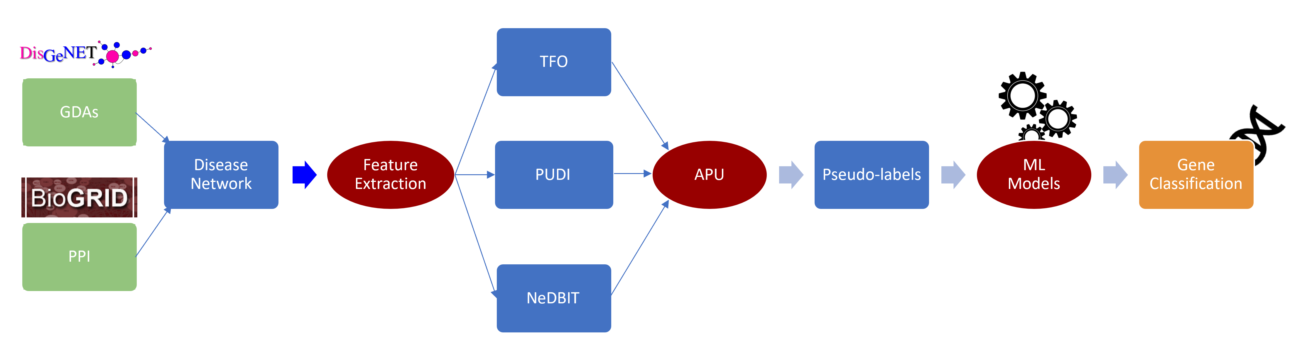
Figure 1: The complete NIAPU pipeline. PPI and GDAs are used to obtain a disease-related network. Features are extracted (Section 2.3) and APU is applied (Section 2.2) to assign new labels to train ML algorithms for the final gene classification. The new labels can be used for disease gene-discovery purposes (Section 3.3).

3.1 NeDBIT classification performances

The effectiveness of the NeDBIT features is tested by comparing NIAPU against the implementation of the APU labeling algorithm with two different sets of features: the first (PUDI) computed following Yang et al., 2012 is based on topological features (originally taken from Xu and Li, 2006) and functional information based on the semantic similarity of GO terms (originally taken from Wang et al., 2007), the second (TFO) includes simple topological, functional, and ontological features (see Supplementary Files 2 and 3). The comparison is carried out in terms of out-of-sample classification performance, namely the ten datasets detailed in Section 2.1 were split into training set (70%) and test set (30%), keeping class balance. Then, we trained the three ML algorithms defined in Step 6 of Section 2.2 for the three different applications of the APU algorithm.

Results related to malignant neoplasm of breast disease are reported in Figure 2 in terms of confusion matrices. The comparison among TFO, PUDI, and NeDBIT features shows that the latter are far superior to the others. The joint usage of APU and NeDBIT features (NIAPU) succeeded in discriminating the class P from the rest of the genes and better separating the pseudo-classes LP, WN, LN, and RN.

Regarding the pseudo-classes, the identification performances were also satisfying using TFO and PUDI features, even if with a drop in accuracy compared to NeDBIT. This highlights the effectiveness of the APU label assignment. RF and MLP delivered the best performances. Regarding SVM, LN samples were sometimes misclassified as either WN or RN.

Overall, for P and RN classes, the NIAPU classification is almost perfect since NeDBIT features allow those classes to be properly separated from the others since they grasp the topological aspects of the set of seed genes as a whole, assigning lower and lower weights to genes that are progressively “far” from the set of seed genes. For the rest of the classes, the performances are good but some genes are misclassified. This is due to the label assignment via quantiles, which obviously introduces some arbitrary noise at the boundary of such quantiles.

Results related to the other diseases are provided in Supplementary File 2, along with the results of a five-fold cross-validation study carried out for the three sets of features.

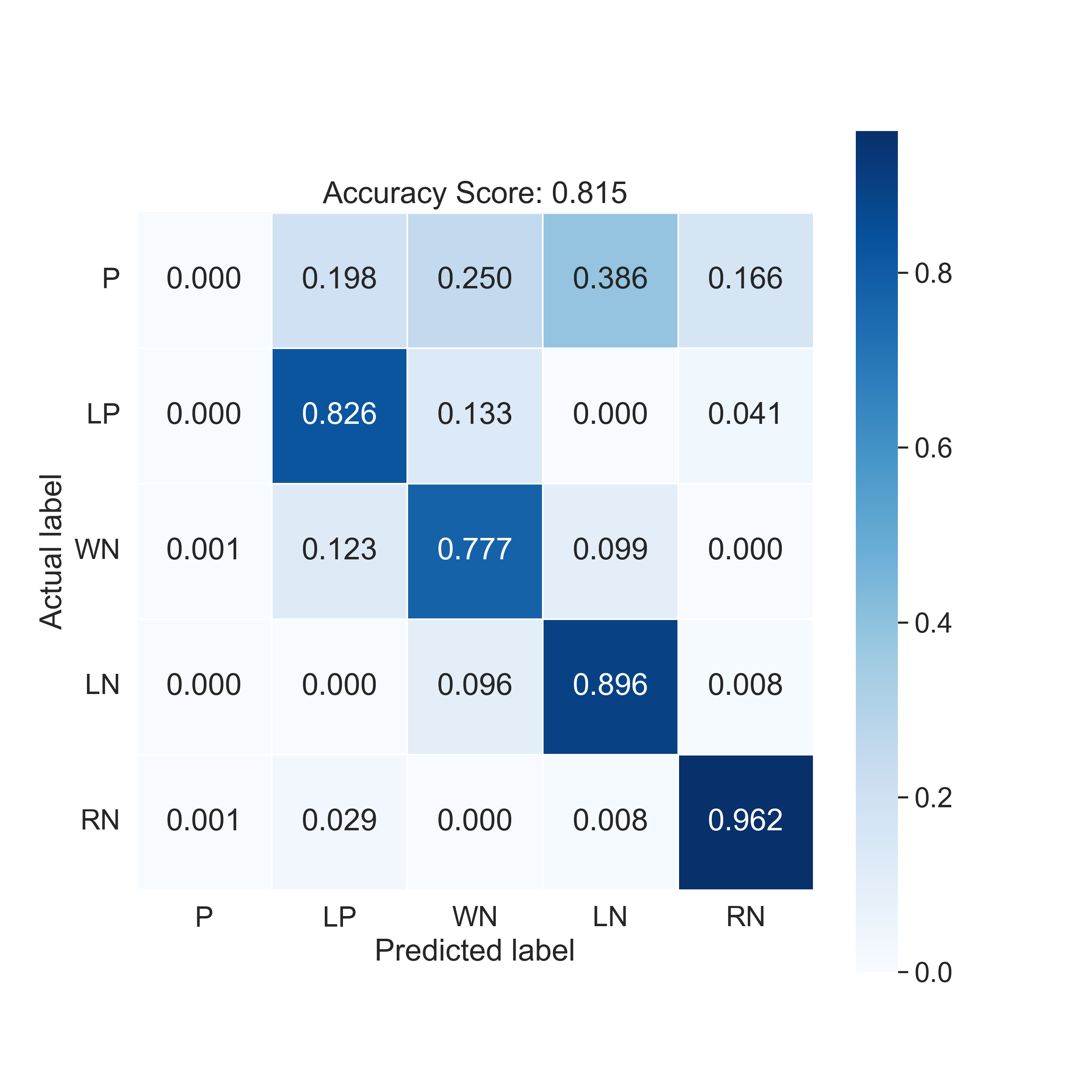
(a) MLP + TFO features

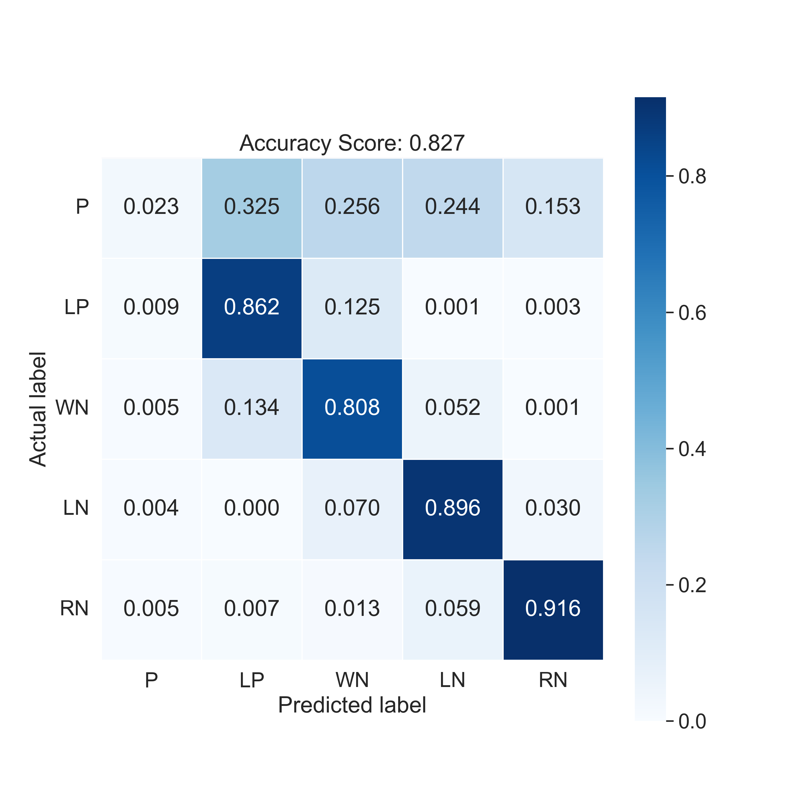
(b) MLP + PUDI features

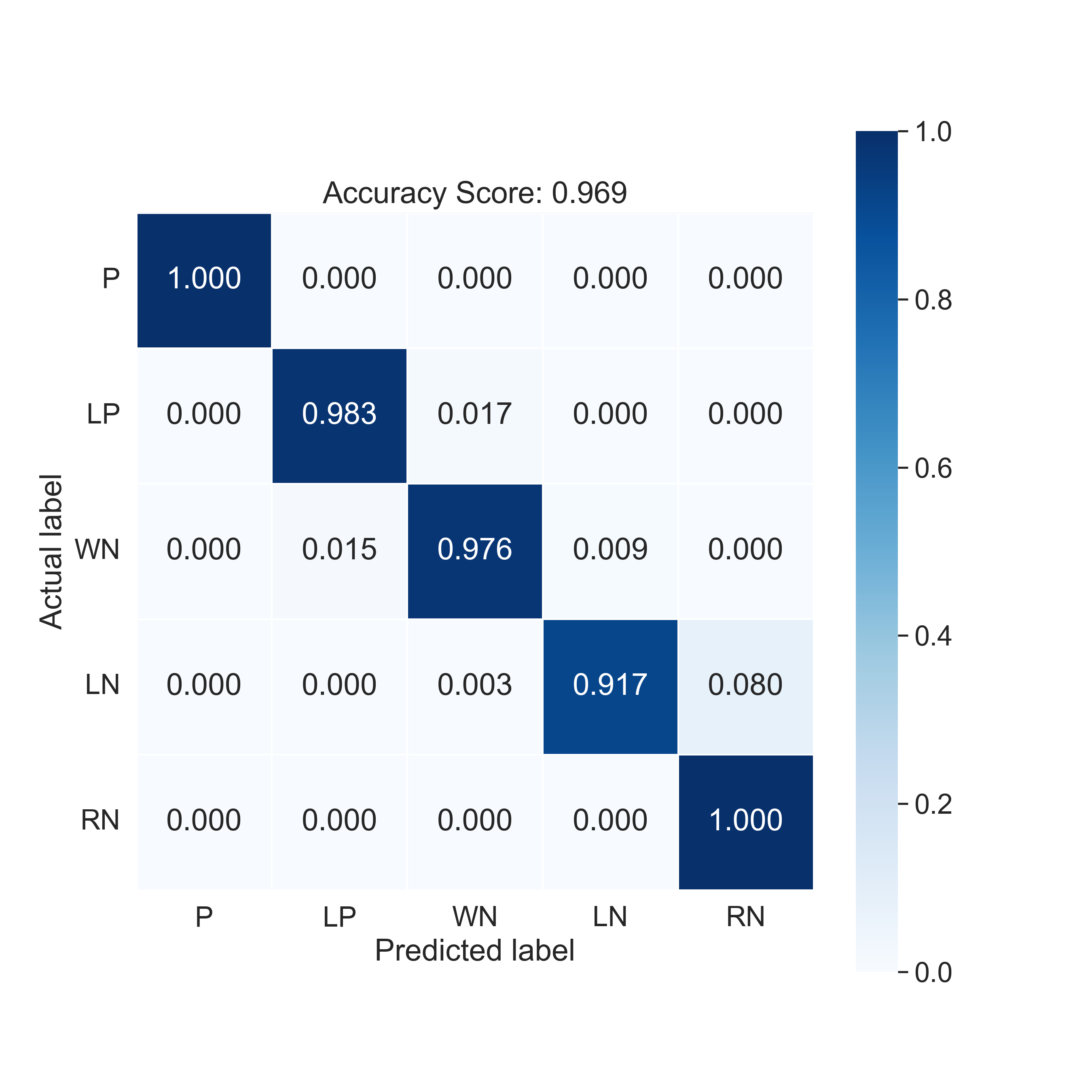
(c) MLP + NeDBIT features

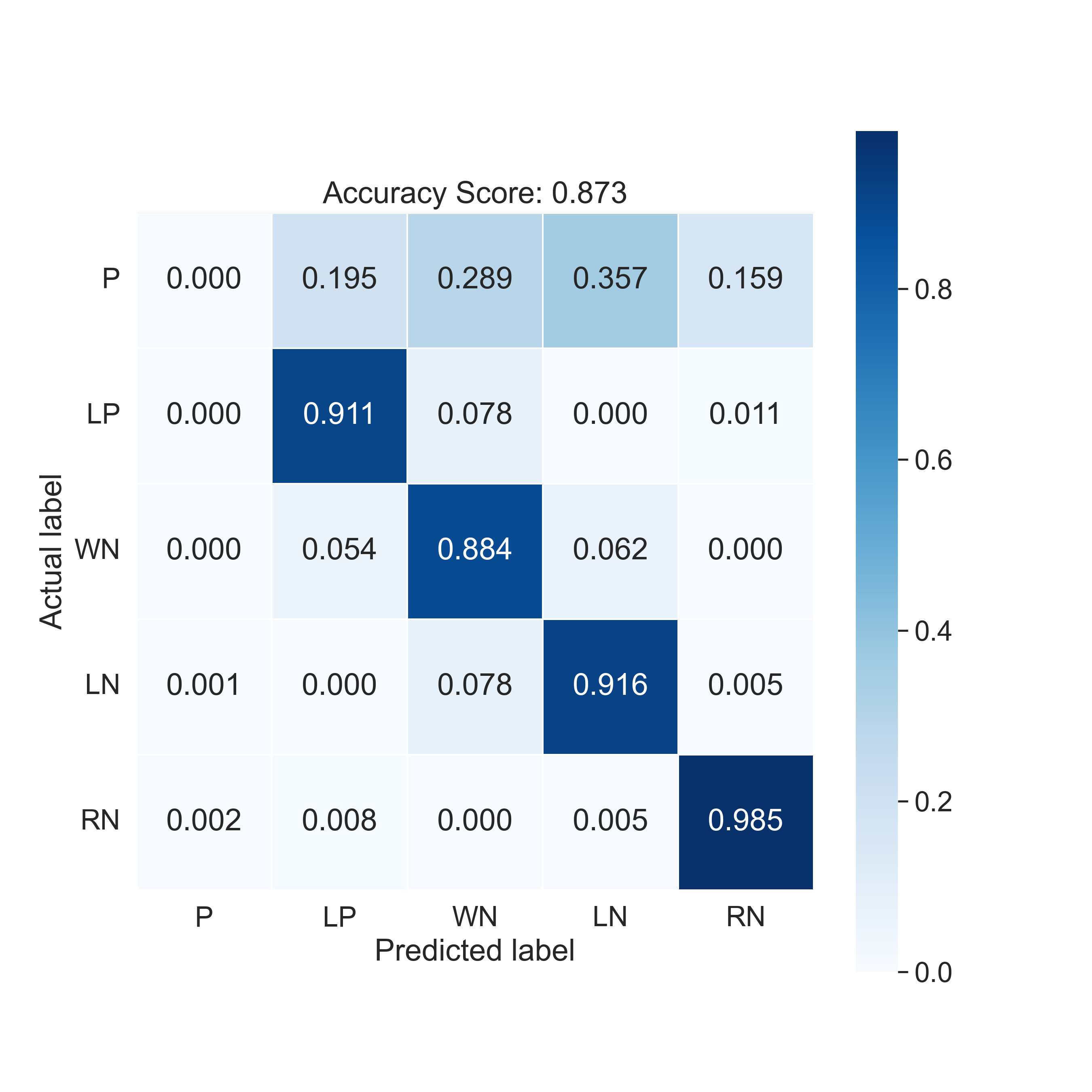
(d) RF + TFO features

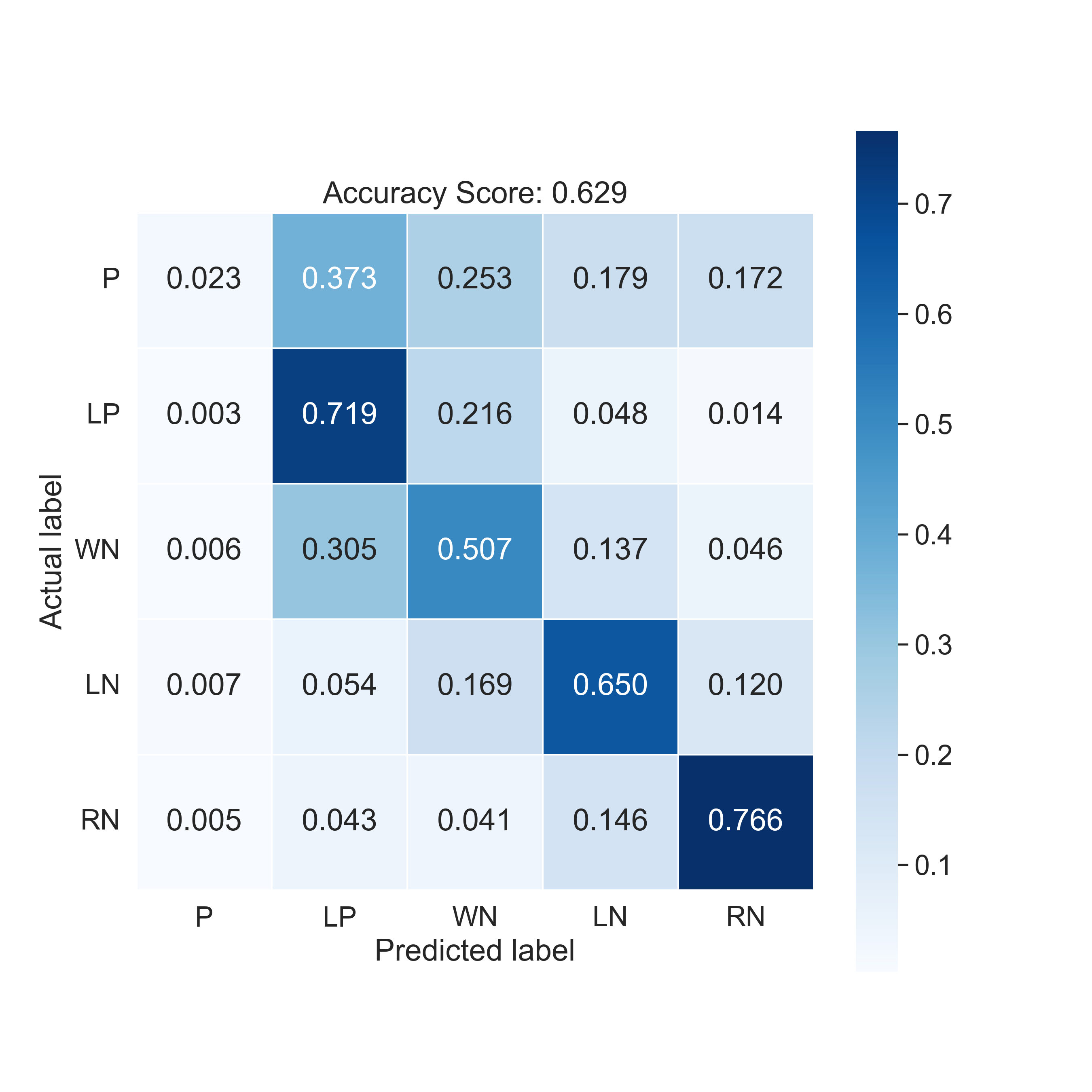
(e) RF + PUDI features

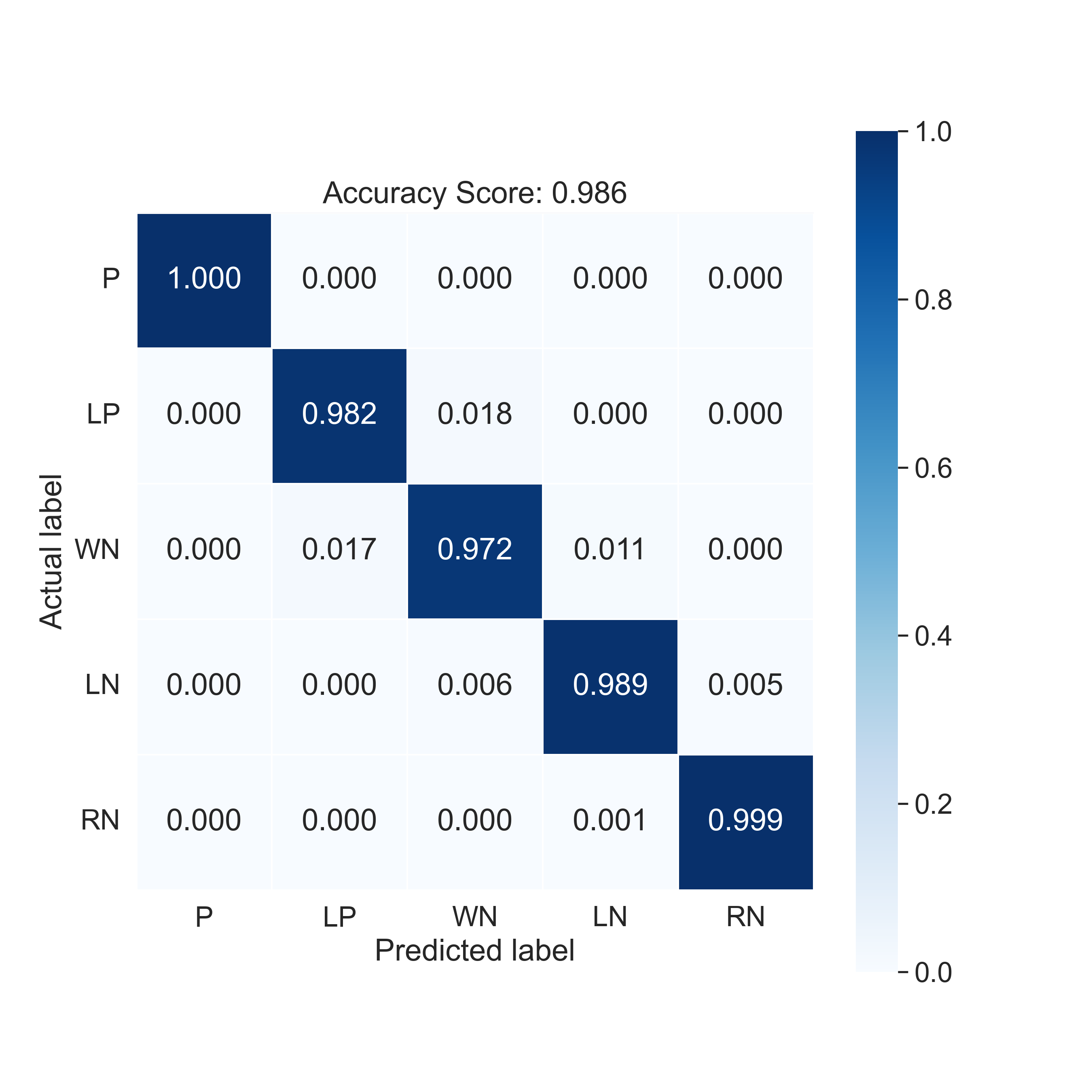
(f) RF + NeDBIT features

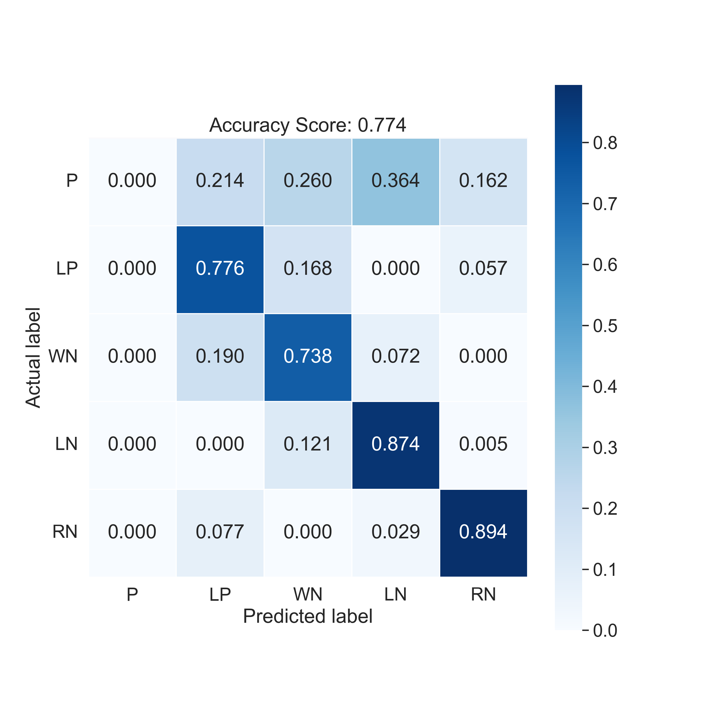
(g) SVM + TFO features

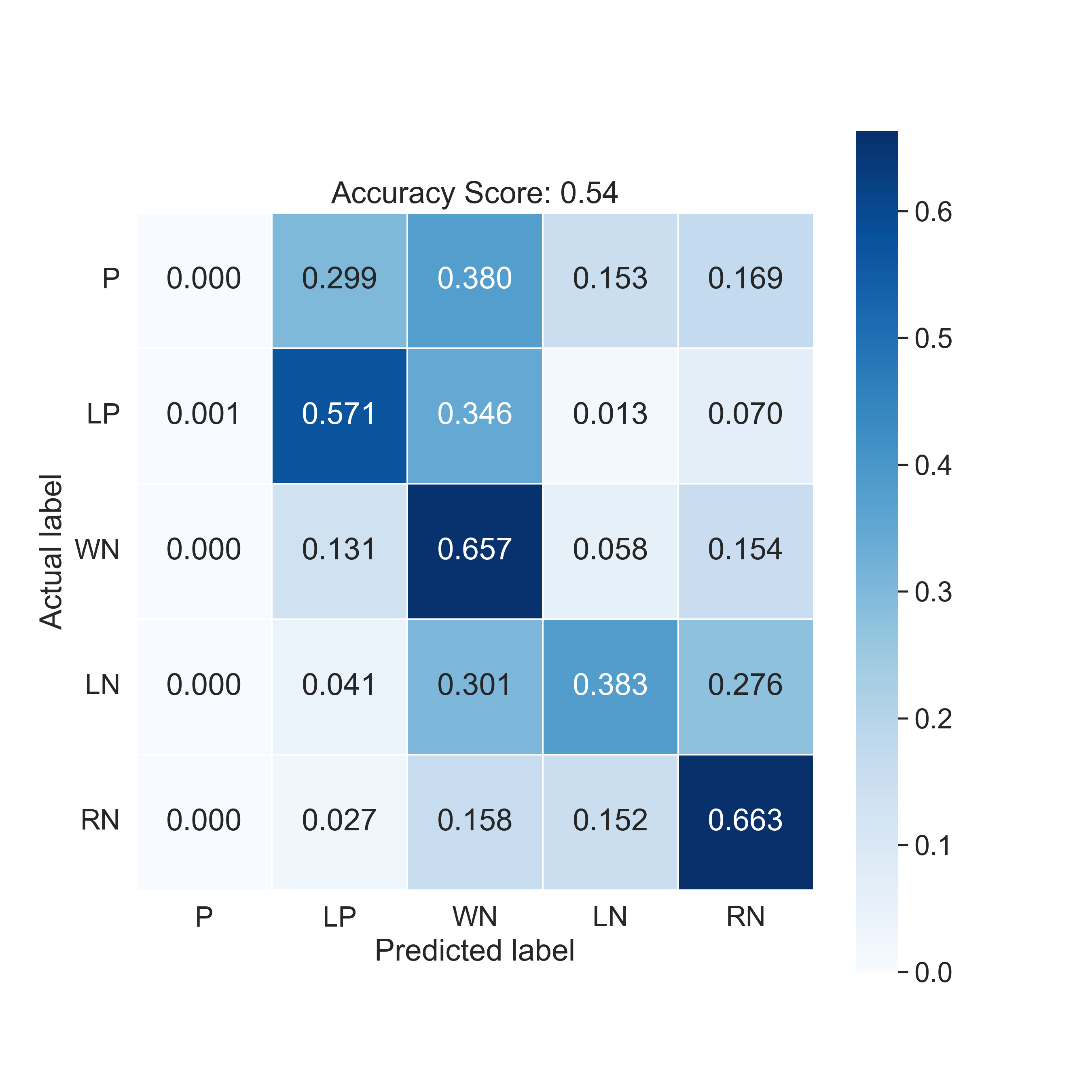
(h) SVM + PUDI features

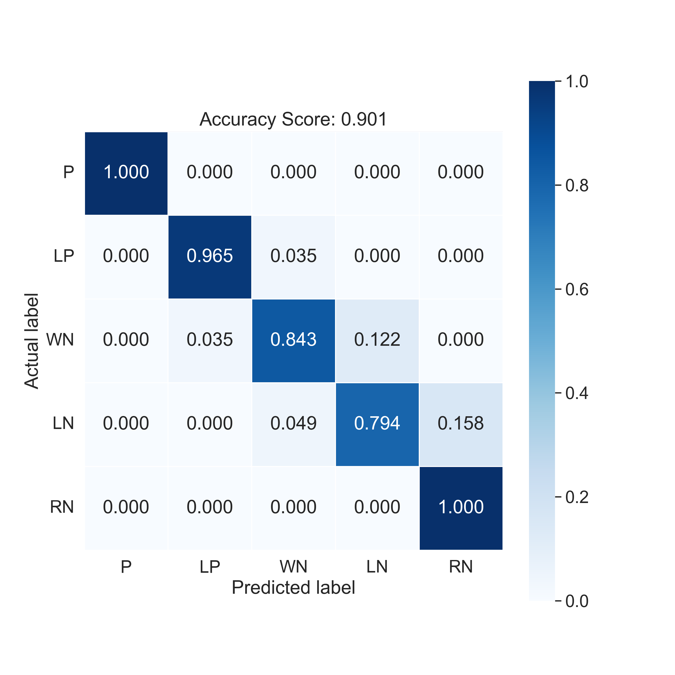
(i) SVM + NeDBIT features

Figure 2: Confusion matrices for multi-class classification on malignant neoplasm of breast (C0006142). The APU labeling and the newly defined NeDBIT features allow for a better and clear distinction of the P class and the pseudo-classes.

3.2 NIAPU performances in disease gene identification

We tested the ability of NIAPU to identify new candidate genes. We performed a validation by excluding the 20% of seed genes, setting them as unlabeled both in the computation of the NeDBIT features and in the APU labeling algorithm. We repeated the procedure five times with non-overlapping gene sets. We investigated whether NIAPU was able to properly classify the removed positive genes as LP. For brevity, the results for malignant neoplasm of breast only are reported in Table 1 (other diseases in Supplementary File 2). On average, around 46% of unlabeled seed genes fell in the LP class, while the rest fell in a decreasing classification trend toward the RN class. We also observed a clear correspondence between the labeling and the association score: the higher the score, the more likely the gene is to be found in the LP class. This underlines the influence of scores on the NeDBIT features. Analogous results can be found in Supplementary File 2 for the remaining diseases.

Aggregated results related to ML classification for malignant neoplasm of breast are reported in Table 2. All the classes were identified by RF and MLP with high scores, while SVM reported lower metrics, particularly with regard to the LN class. Therefore, NIAPU turned out to be robust also in more challenging settings with reduced seed gene sets.

Table 1: Labeling of the unlabeled seed genes by NIAPU for malignant neoplasm of breast (C0006142). Results are intended as average with standard deviation over the five runs (GDAS: association score $\mathbf{S}$).

label % genes # genes GDAS mean GDAS median GDAS mode LP 45.659 ± 1.362 93.6 ± 2.793 0.383 ± 0.016 0.346 ± 0.019 0.32 ± 0.045 WN 27.415 ± 0.636 56.2 ± 1.304 0.343 ± 0.013 0.318 ± 0.011 0.3 ± 0.0 LN 17.659 ± 4.436 36.2 ± 9.094 0.324 ± 0.012 0.303 ± 0.004 0.3 ± 0.0 RN 9.268 ± 3.65 19.0 ± 7.483 0.322 ± 0.013 0.303 ± 0.004 0.3 ± 0.0

Table 2: Classification scores as pooled mean and standard deviation (over all the diseases). Five runs were performed for each disease, masking out 20% of seed genes.

label	precision	recall	F1 score
MLP
P	0.994 ± 0.011	0.998 ± 0.007	0.996 ± 0.007
LP	0.972 ± 0.013	0.972 ± 0.016	0.972 ± 0.012
WN	0.955 ± 0.02	0.915 ± 0.022	0.933 ± 0.019
LN	0.835 ± 0.021	0.744 ± 0.042	0.782 ± 0.019
RN	0.731 ± 0.037	0.86 ± 0.036	0.788 ± 0.024
macro avg	0.898 ± 0.008	0.898 ± 0.007	0.894 ± 0.008
weighted avg	0.884 ± 0.009	0.876 ± 0.009	0.876 ± 0.009
accuracy	0.876 ± 0.009
RF
P	1.0 ± 0.0	1.0 ± 0.0	1.0 ± 0.0
LP	0.984 ± 0.005	0.984 ± 0.005	0.984 ± 0.005
WN	0.977 ± 0.007	0.976 ± 0.007	0.977 ± 0.006
LN	0.982 ± 0.005	0.986 ± 0.004	0.984 ± 0.004
RN	0.991 ± 0.003	0.987 ± 0.004	0.989 ± 0.003
macro avg	0.987 ± 0.003	0.987 ± 0.003	0.987 ± 0.003
weighted avg	0.984 ± 0.004	0.984 ± 0.004	0.984 ± 0.004
accuracy	0.984 ± 0.004
SVM
P	0.998 ± 0.004	1.0 ± 0.0	0.999 ± 0.002
LP	0.845 ± 0.043	0.719 ± 0.071	0.767 ± 0.032
WN	0.635 ± 0.135	0.726 ± 0.108	0.625 ± 0.102
LN	0.625 ± 0.191	0.559 ± 0.026	0.419 ± 0.025
RN	0.366 ± 0.224	0.5 ± 0.004	0.38 ± 0.011
macro avg	0.694 ± 0.066	0.701 ± 0.013	0.638 ± 0.022
weighted avg	0.641 ± 0.077	0.642 ± 0.017	0.568 ± 0.029
accuracy	0.642 ± 0.017

3.3 NIAPU vs. other disease gene identification tools

We compared the predictive performance in the identification of candidate disease genes of NIAPU against known gene discovery algorithms, namely DIAMOnD (Ghiassian et al., 2015), Markov clustering (MCL) (Enright et al., 2002; Sun et al., 2011), random walk with restart (RWR) (Köhler et al., 2008; Valdeolivas et al., 2019), two variants of GUILD (Guney and Oliva, 2012), one exploiting the NetCombo measure and the other based on Functional Flow (fFlow) (Nabieva et al., 2005), and ToppGene (Chen et al., 2009a) (relying on the implementation provided by the GUILD software). See Supplementary File 2 for a detailed description of these algorithms. For this analysis, we relied on the extended GDA dataset provided by DisGeNET. We assigned the labels using NIAPU on the curated version of the dataset and then investigated whether the seed genes contained in the extended version (but not in the curated one) fell into the LP class. We considered the ranking retrieved by NIAPU at different quantile thresholds.

In Figure 3, we report the results of this comparison in terms of F1 score. Most of the time, our methodology outperformed or was at par with the state-of-the-art algorithms for disease gene identification, being often the best-performing method when looking for a large number of candidate genes and of comparable performances for lower ones. Indeed, DIAMOnD performs at its best when considering a low ratio (10-20%) of predicted genes, while NIAPU shows good performances both for low and high percentages of candidate genes, outperforming DIAMOnD in the latter case. In fact, as stated by the authors themselves, DIAMOnD becomes unreliable when exceeding 200 predicted genes (Ghiassian et al., 2015).

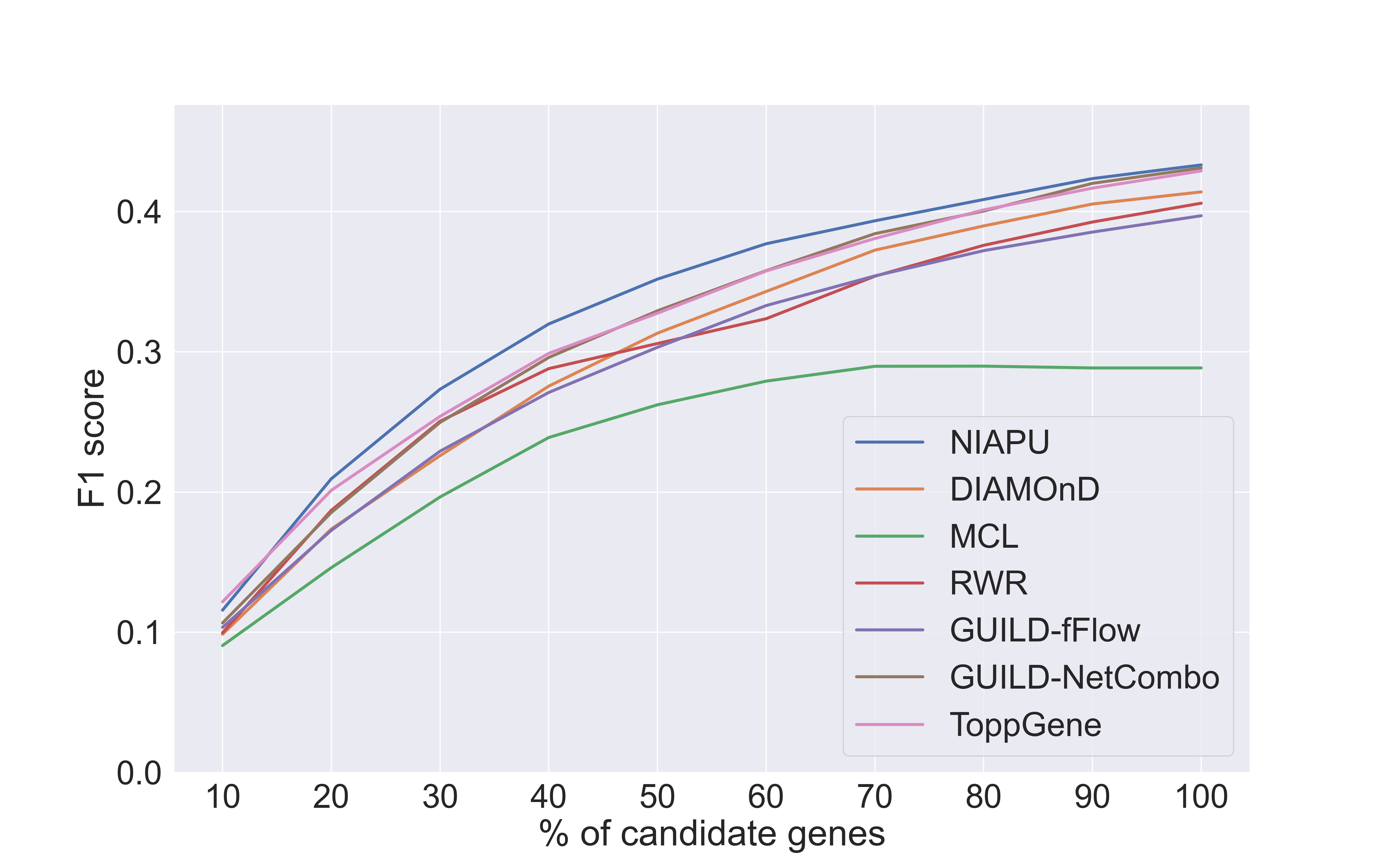
(a) Malignant neoplasm of breast (C0006142)

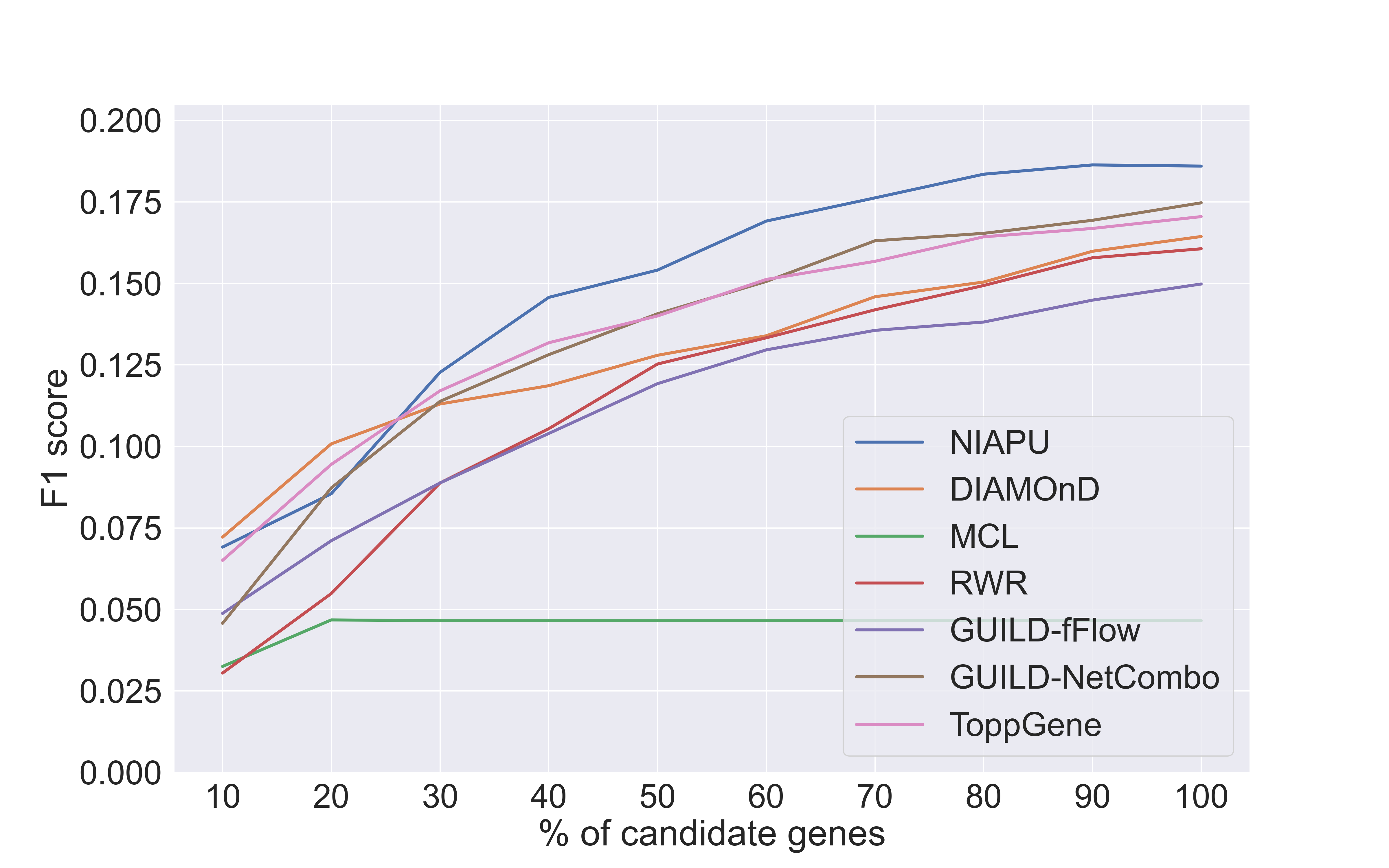
(b) Schizophrenia (C0036341)

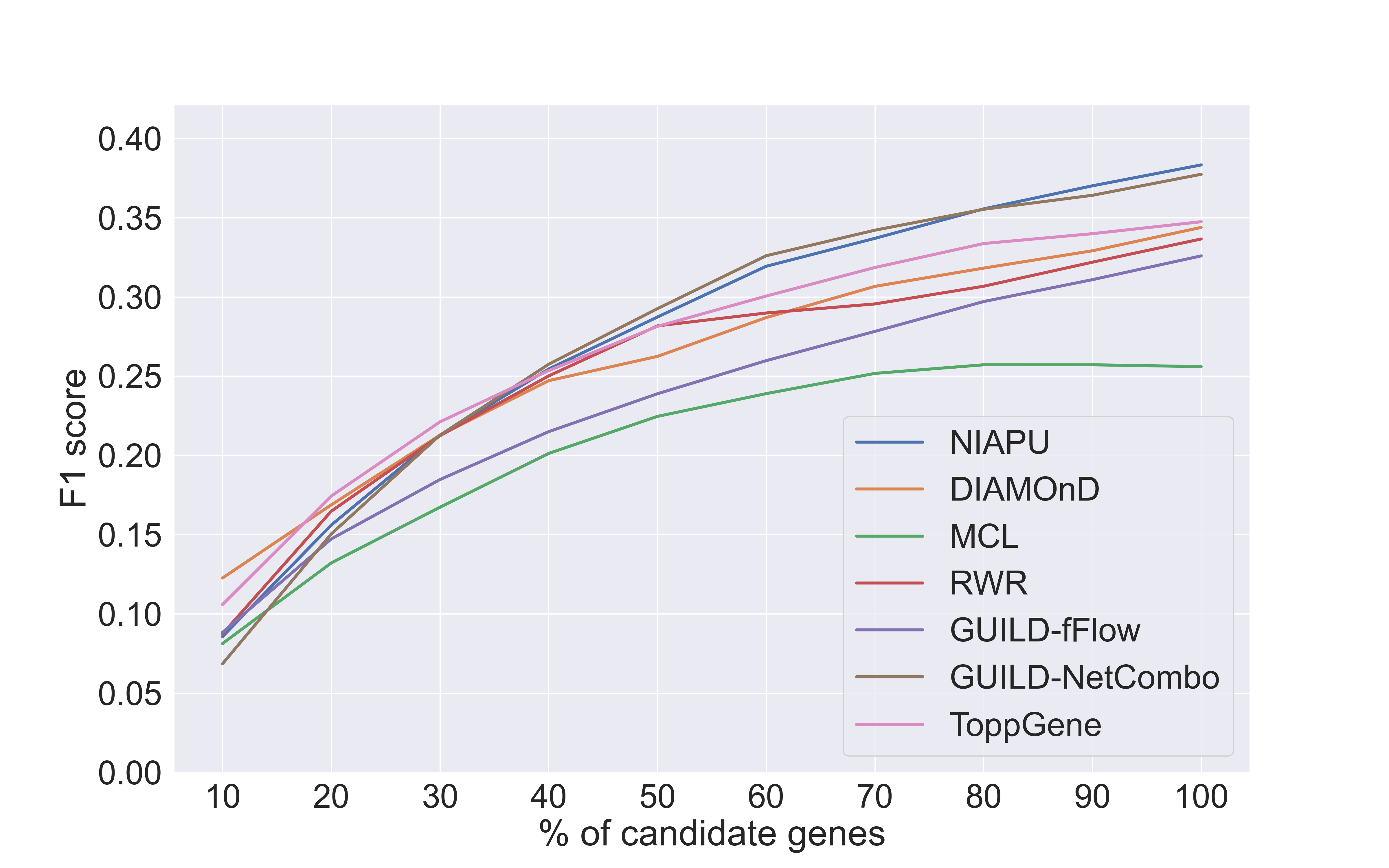
(c) Colorectal carcinoma (C0009402)

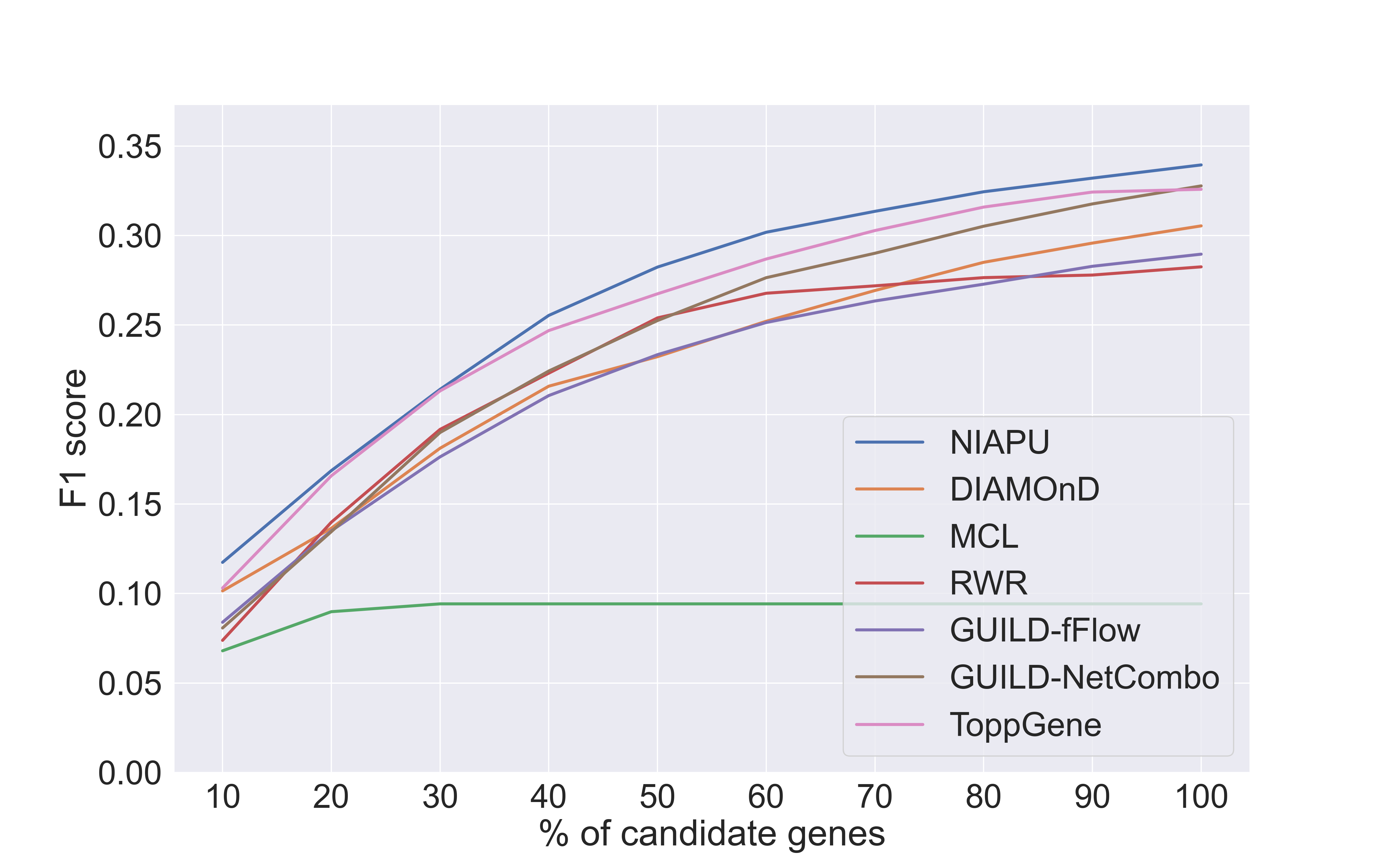
(d) Malignant neoplasm of prostate (C0376358)

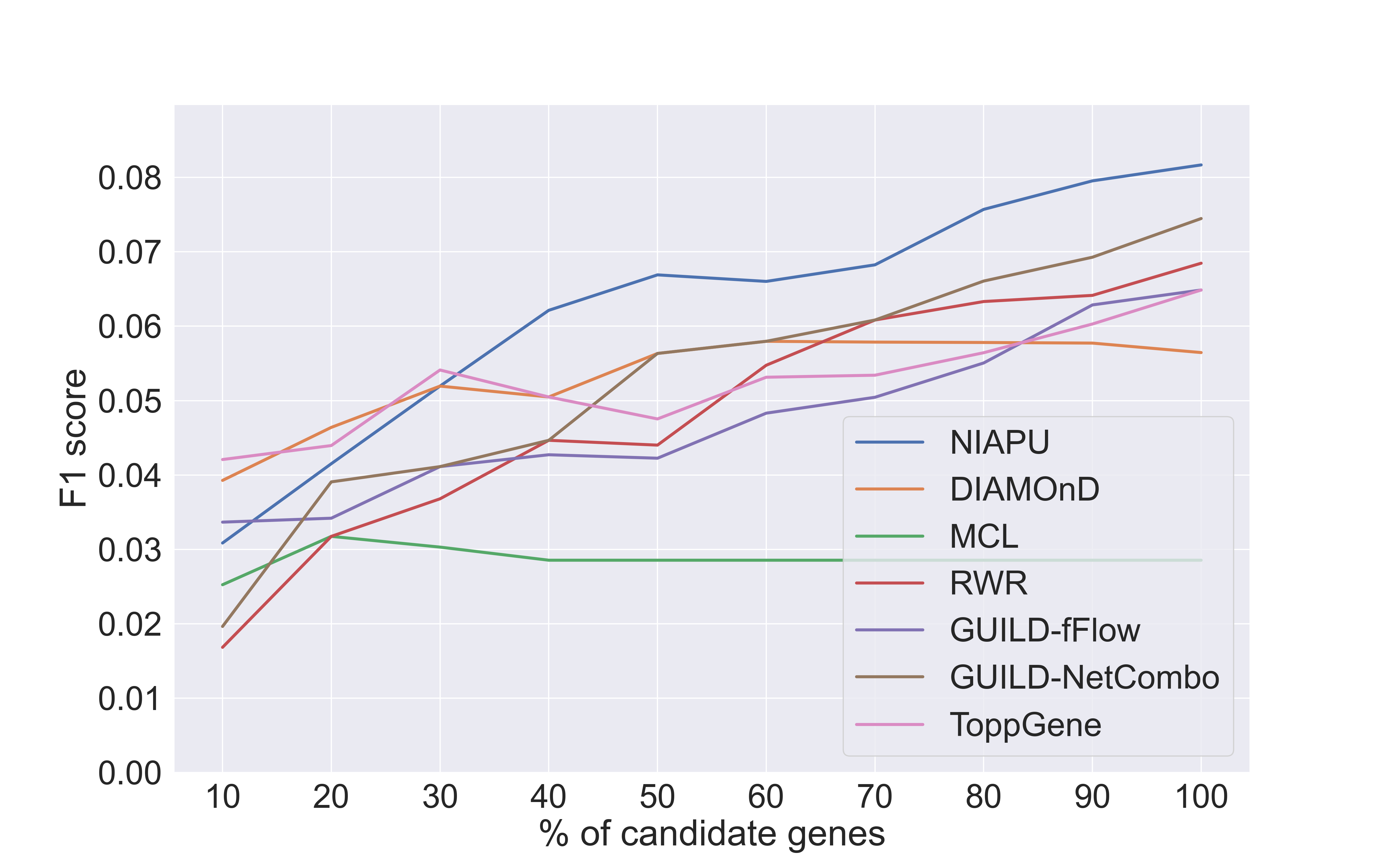
(e) Bipolar disorder (C0005586)

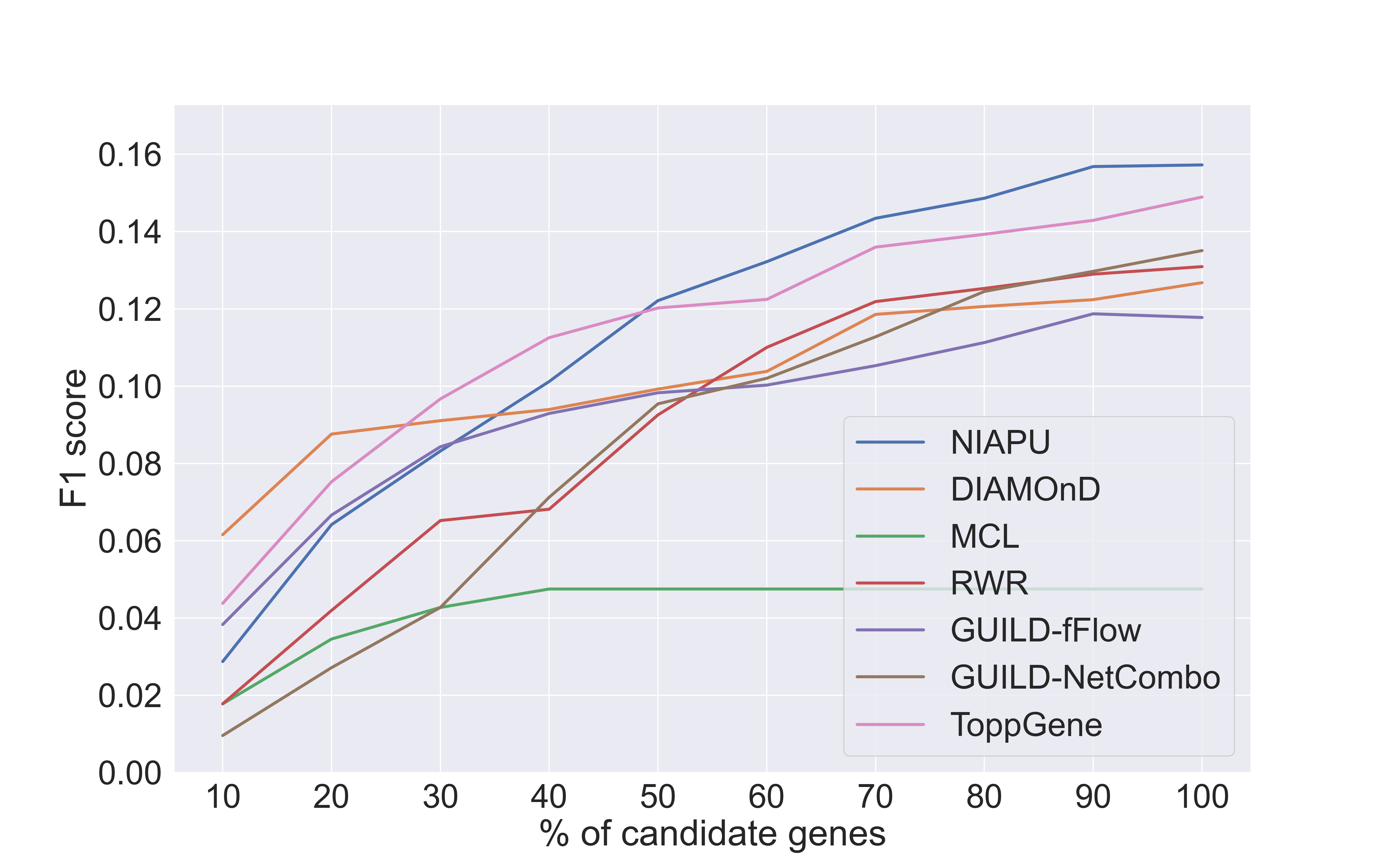
(f) Depressive disorder (C0011581)

Figure 3: Gene discovery performances in terms of F1 score. Results are reported for six diseases for increasing numbers of candidate genes considered as a percentage of the total number of associated genes in the extended dataset, which is different for each disease. The rest of the diseases can be found in Supplementary File 2.

3.4 Enrichment analysis

For a further evaluation of our results, for each of the ten diseases considered, we performed a gene ontology/pathway/disease enrichment analysis of the first 100 predicted genes in the LP class from the validation on the extended GDA dataset. This analysis was performed using Enrichr (Chen et al., 2013; Kuleshov et al., 2016; Xie et al., 2021).

The selected LP genes do not correspond to any of the curated GDA disease genes; therefore, among the enriched diseases, we cannot expect to find the same disease for which the gene discovery process is carried out. Instead, among the enriched terms (diseases, GO terms, or pathways), we should be able to find diseases and biological processes that are somehow related to the disease under scrutiny.

We report the enrichment analysis results in Table 3. In particular, we present the top enriched diseases or biological processes for each analyzed disease, together with references to literature that endorse such relevant links.

Although not conclusive, the fact that there is evidence in literature of links and shared biological mechanisms between the analyzed diseases and enriched diseases is additional proof of the validity and efficacy of the disease gene discovery process.

Table 3: Enrichment analysis of the LP genes predicted for the ten diseases of interest. The top enriched diseases and GO terms are reported, along with notes about disease relationships and main reference articles.

Disease Enriched disease/GO Relationship Reference C0036341 Schizophrenia KEGG GO:0042981 Regulation of apoptotic processes Apoptotic engulfment pathway involved in schizophrenia (increased risk) Chen et al.,2009b C0005586 Bipolar disorder (BD) KEGG GO:0042981 Regulation of apoptotic processes Observed relationship between mitochondrial dynamics and dysfunction and the apoptotic pathway activation and the pathophysiology of BD Scaini et al.,2017 C0006142 Malignant neoplasm of breast Leukaemia Therapy-related myeloid neoplasms may be part of a cancer-risk syndrome involving breast cancer Valentini et al.,2011 C0009402 Colorectal carcinoma (CRC) Ovarian cancer (OC) GCNT3 might constitute a prognostic factor also in OC and emerges as an essential glycosylation-related molecule in CRC and OC progression Fernández et al.,2018 Parkinson Neurobiological investigations suggest that depression in Parkinson’s disease may be mediated by dysfunction in mesocortical/prefrontal reward, motivational, and stress-response systems Cummings,1992 C0011581 Depressive disorder GO:0043066 Negative regulation of apoptotic processes Evidence of local inflammatory, apoptotic, and oxidative stress in major depressive disorder Shelton et al.,2011 C0023893 Liver cirrhosis Parkinson Parkinson’s disease among the neurological complications in advanced liver cirrhosis mediated by manganese Mehkari et al.,2020 C0376358 Prostate cancer Melanoma Diagnoses of cutaneous melanoma may be associated with prostate cancer incidence Cole-Clark et al.,2018 C3714756 Intellectual disability Dementia People with intellectual disability are at higher risk of dementia than the general population Zigman and Lott,2007 Ovarian cancer (OC) Alcohol consumption might be associated with the risk of OC in specific populations or in studies with specific characteristics Yan-Hong et al.,2015 C0860207 Chronic alcoholic intoxication KEGG Estrogen signaling pathway Association of increased estrogen level and increased alcohol use in females Erol et al.,2019 C0001973 Drug-induced liver disease Leigh Syndrome (LS) Valproate, listed as a cause of drug-induced acute liver failure, can cause mitochondrial dysfunction and should be avoided in LS patients Lee and Chiang,2021

4 Discussions and conclusions

In this paper, we presented the NIAPU algorithm, which fits the typical problem of the computational identification of previously unknown disease genes in the context of positive-unlabeled learning. The advantage of the proposed method is that it allows accurate characterization of the positive samples (P set) – via the NeDBIT features – and refined control of the likely positive samples (LP set) – via the APU labeling procedure – which, extracted from the set of unlabeled elements, contains, with the highest probability, elements related to the disease of interest. Moreover, NIAPU turned out to be an effective labeling procedure, allowing machine learning models to be trained appropriately and deliver highly accurate classification performances. As for disease gene identification, NIAPU proved to be efficient in two different experiments. In the first one, masking out a subset of seed genes, it turned out that ~46% of those fell in the LP class. In the second one, assigning labels using NIAPU on the curated version of the DisGeNET dataset and then searching for the seed genes of the extended version only, the predictive performance of the NIAPU algorithm outperformed or was at par with the state-of-the-art algorithms for disease gene discovery.

It is worth noting that the NeDBIT features are designed to be able to use link-weighted and node-weighted graphs and that, by having increasingly accurate PPIs, we expect increasingly good results from the application of NIAPU. On the other hand, NIAPU methodology is clearly influenced by the reliability of seed genes, the association score assigned to them, and the background network topology (here, the PPI network and its reliability).

Indeed, GDA datasets may be affected by disease-gene association bias due to the quantity of research on a given disease/trait. In this regard, a recent systematic review (De Magalhães, 2021) demonstrated that 87.7% of all genes could be associated with cancer. This indicates that given the massive amount of research focused on cancer, which also applies to other types of diseases, the definition “associated with” is to be checked carefully and critically.

The usage of datasets that are as error-free, unbiased, and reliable as possible (e.g., using an interactome validated in the specific pathological context, possibly with weighted PPIs) could potentially improve the classification performance of the method. In this regard, it is worth mentioning that an algorithm with the same theoretical ground of NIAPU has been applied in different contexts (e.g., nephrology, gastroenterology, rare diseases) (Shahini et al., 2022a, b), paying particular attention to the selection of seed genes and reference interactomes.

Funding

This work has been partially supported by the ERC Advanced Grant 788893 AMDROMA “Algorithmic and Mechanism Design Research in Online Markets”, the EC H2020RIA project “SoBigData++” (871042), the MIUR PRIN project ALGADIMAR “Algorithms, Games, and Digital Markets”, and by the CNR project DIT.AD021.161.001 / Analisi probabilistica di dataset biologici e network dynamics.

References

- Baronchelli and Loreto (2006) Baronchelli, A. and Loreto, V. (2006). Ring structures and mean first passage time in networks. Physical Review E, 73(2), 026103.
- Bekker and Davis (2020) Bekker, J. and Davis, J. (2020). Learning from positive and unlabeled data: a survey. Machine Learning, 109(4), 719–760.
- Bravo et al. (2014) Bravo, A. et al. (2014). A knowledge-driven approach to extract disease-related biomarkers from the literature. BioMed research international, 2014.
- Bravo et al. (2015) Bravo, À. et al. (2015). Extraction of relations between genes and diseases from text and large-scale data analysis: implications for translational research. BMC bioinformatics, 16(1), 1–17.
- Breiman (2001) Breiman, L. (2001). Random forests. Machine learning, 45(1), 5–32.
- Bundschus et al. (2008) Bundschus, M. et al. (2008). Extraction of semantic biomedical relations from text using conditional random fields. BMC bioinformatics, 9(1), 1–14.
- Bundschus et al. (2010) Bundschus, M. et al. (2010). Digging for knowledge with information extraction: a case study on human gene-disease associations. In Proceedings of the 19th ACM international conference on Information and knowledge management, pages 1845–1848.
- Can et al. (2005) Can, T. et al. (2005). Analysis of protein-protein interaction networks using random walks. In Proceedings of the 5th international workshop on Bioinformatics, pages 61–68.
- Carlin et al. (2017) Carlin, D. E. et al. (2017). Network propagation in the cytoscape cyberinfrastructure. PLoS computational biology, 13(10), e1005598.
- Chen et al. (2013) Chen, E. Y. et al. (2013). Enrichr: interactive and collaborative html5 gene list enrichment analysis tool. BMC bioinformatics, 14(1), 1–14.
- Chen et al. (2009a) Chen, J. et al. (2009a). Disease candidate gene identification and prioritization using protein interaction networks. BMC bioinformatics, 10(1), 1–14.
- Chen et al. (2009b) Chen, X. et al. (2009b). Apoptotic engulfment pathway and schizophrenia. PLoS One, 4(9), e6875.
- Claesen et al. (2015) Claesen, M. et al. (2015). A robust ensemble approach to learn from positive and unlabeled data using svm base models. Neurocomputing, 160, 73–84.
- Cole-Clark et al. (2018) Cole-Clark, D. et al. (2018). An initial melanoma diagnosis may increase the subsequent risk of prostate cancer: Results from the New South Wales Cancer Registry. Sci Rep, 8(1), 7167.
- Cortes and Vapnik (1995) Cortes, C. and Vapnik, V. (1995). Support-vector networks. Machine learning, 20(3), 273–297.
- Cummings (1992) Cummings, J. L. (1992). Depression and Parkinson’s disease: a review. Am J Psychiatry, 149(4), 443–454.
- De Magalhães (2021) De Magalhães, J. P. (2021). Every gene can (and possibly will) be associated with cancer. Trends in Genetics.
- Doncheva et al. (2012) Doncheva, N. T. et al. (2012). Recent approaches to the prioritization of candidate disease genes. WIREs Systems Biology and Medicine, 4(5), 429–442.
- Drucker et al. (1997) Drucker, H. et al. (1997). Support vector regression machines. Advances in neural information processing systems, 9, 155–161.
- Elkan and Noto (2008) Elkan, C. and Noto, K. (2008). Learning classifiers from only positive and unlabeled data. In Proceedings of the 14th ACM SIGKDD international conference on Knowledge discovery and data mining, pages 213–220.
- Enright et al. (2002) Enright, A. J. et al. (2002). An efficient algorithm for large-scale detection of protein families. Nucleic Acids Res, 30(7), 1575–1584.
- Erol et al. (2019) Erol, A. et al. (2019). Sex hormones in alcohol consumption: a systematic review of evidence. Addiction biology, 24(2), 157–169.
- Fernández et al. (2018) Fernández, L. P. et al. (2018). The role of glycosyltransferase enzyme GCNT3 in colon and ovarian cancer prognosis and chemoresistance. Sci Rep, 8(1), 8485.
- Ghiassian et al. (2015) Ghiassian, S. D. et al. (2015). A DIseAse MOdule Detection (DIAMOnD) algorithm derived from a systematic analysis of connectivity patterns of disease proteins in the human interactome. PLoS Comput Biol, 11(4), e1004120.
- Guney and Oliva (2012) Guney, E. and Oliva, B. (2012). Exploiting protein-protein interaction networks for genome-wide disease-gene prioritization. PLoS One, 7(9), e43557.
- Hastie et al. (2001) Hastie, T. et al. (2001). The elements of statistical learning. springer series in statistics. In :. Springer.
- Janyasupab et al. (2021) Janyasupab, P. et al. (2021). Network diffusion with centrality measures to identify disease-related genes. Math Biosci Eng, 18(3), 2909–2929.
- Ke et al. (2018) Ke, T. et al. (2018). A biased least squares support vector machine based on mahalanobis distance for pu learning. Physica A: Statistical Mechanics and its Applications, 509, 422–438.
- Köhler et al. (2008) Köhler, S. et al. (2008). Walking the interactome for prioritization of candidate disease genes. The American Journal of Human Genetics, 82(4), 949–958.
- Kuleshov et al. (2016) Kuleshov, M. V. et al. (2016). Enrichr: a comprehensive gene set enrichment analysis web server 2016 update. Nucleic acids research, 44(W1), W90–W97.
- Lancour et al. (2018) Lancour, D. et al. (2018). One for all and all for One: Improving replication of genetic studies through network diffusion. PLoS Genet, 14(4), e1007306.
- Lee and Chiang (2021) Lee, I.-C. and Chiang, K.-L. (2021). Clinical diagnosis and treatment of leigh syndrome based on surf1: Genotype and phenotype. Antioxidants, 10(12), 1950.
- Li and Patra (2010a) Li, Y. and Patra, J. C. (2010a). Genome-wide inferring gene–phenotype relationship by walking on the heterogeneous network. Bioinformatics, 26(9), 1219–1224.
- Li and Patra (2010b) Li, Y. and Patra, J. C. (2010b). Integration of multiple data sources to prioritize candidate genes using discounted rating system. BMC bioinformatics, 11(1), 1–10.
- Liu et al. (2003) Liu, B. et al. (2003). Building text classifiers using positive and unlabeled examples. In Proceedings of the Third IEEE International Conference on Data Mining, ICDM ’03, page 179, USA. IEEE Computer Society.
- Mehkari et al. (2020) Mehkari, Z. et al. (2020). Manganese, a Likely Cause of ’Parkinson’s in Cirrhosis’, a Unique Clinical Entity of Acquired Hepatocerebral Degeneration. Cureus, 12(9), e10448.
- Mordelet and Vert (2014) Mordelet, F. and Vert, J. P. (2014). A bagging svm to learn from positive and unlabeled examples. Pattern Recogn. Lett., 37, 201–209.
- Nabieva et al. (2005) Nabieva, E. et al. (2005). Whole-proteome prediction of protein function via graph-theoretic analysis of interaction maps. Bioinformatics, 21(suppl_1), i302–i310.
- Nitsch et al. (2010) Nitsch, D. et al. (2010). Candidate gene prioritization by network analysis of differential expression using machine learning approaches. BMC Bioinformatics, 11, 460.
- Opap and Mulder (2017) Opap, K. and Mulder, N. (2017). Recent advances in predicting gene–disease associations. F1000Research, 6, 578.
- Petti et al. (2021) Petti, M. et al. (2021). Moses: A new approach to integrate interactome topology and functional features for disease gene prediction. Genes, 12(11), 1713.
- Picart-Armada et al. (2019) Picart-Armada, S. et al. (2019). Benchmarking network propagation methods for disease gene identification. PLoS Comput Biol, 15(9), e1007276.
- Piñero et al. (2016) Piñero, J. et al. (2016). Disgenet: a comprehensive platform integrating information on human disease-associated genes and variants. Nucleic acids research, page gkw943.
- Piñero et al. (2020) Piñero, J. et al. (2020). The disgenet knowledge platform for disease genomics: 2019 update. Nucleic acids research, 48(D1), D845–D855.
- Piro and Cunto (2012) Piro, R. M. and Cunto, F. D. (2012). Computational approaches to disease-gene prediction: rationale, classification and successes. FEBS Journal, 279(5), 678–696.
- Scaini et al. (2017) Scaini, G. et al. (2017). Perturbations in the apoptotic pathway and mitochondrial network dynamics in peripheral blood mononuclear cells from bipolar disorder patients. Transl Psychiatry, 7(5), e1111.
- Shahini et al. (2022a) Shahini, E. et al. (2022a). Network proximity-based drug repurposing strategy for early and late stages of primary biliary cholangitis. Biomedicines, 10(7), 1694.
- Shahini et al. (2022b) Shahini, E. et al. (2022b). Network proximity-based drug repurposing strategy for primary biliary cirrhosis. DIGESTIVE AND LIVER DISEASE, 54.
- Shelton et al. (2011) Shelton, R. C. et al. (2011). Altered expression of genes involved in inflammation and apoptosis in frontal cortex in major depression. Mol Psychiatry, 16(7), 751–762.
- Silverman et al. (2020) Silverman, E. K. et al. (2020). Molecular networks in Network Medicine: Development and applications. Wiley Interdiscip Rev Syst Biol Med, 12(6), e1489.
- Stark et al. (2006) Stark, C. et al. (2006). Biogrid: a general repository for interaction datasets. Nucleic acids research, 34(suppl_1), D535–D539.
- Sun et al. (2011) Sun, P. G. et al. (2011). Prediction of human disease-related gene clusters by clustering analysis. International journal of biological sciences, 7(1), 61.
- Tieri et al. (2019) Tieri, P. et al. (2019). Network inference and reconstruction in bioinformatics. In S. Ranganathan, M. Gribskov, K. Nakai, and C. Schönbach, editors, Encyclopedia of Bioinformatics and Computational Biology, pages 805–813. Academic Press, Oxford.
- Valdeolivas et al. (2019) Valdeolivas, A. et al. (2019). Random walk with restart on multiplex and heterogeneous biological networks. Bioinformatics, 35(3), 497–505.
- Valentini et al. (2011) Valentini, C. G. et al. (2011). Incidence of acute myeloid leukemia after breast cancer. Mediterr J Hematol Infect Dis, 3(1), e2011069.
- Wang et al. (2007) Wang, J. Z. et al. (2007). A new method to measure the semantic similarity of go terms. Bioinformatics, 23(10), 1274–1281.
- White and Smyth (2003) White, S. and Smyth, P. (2003). Algorithms for estimating relative importance in networks. In Proceedings of the ninth ACM SIGKDD international conference on Knowledge discovery and data mining, pages 266–275.
- Xie et al. (2021) Xie, Z. et al. (2021). Gene set knowledge discovery with enrichr. Curr Protoc, 1(3), e90.
- Xu and Li (2006) Xu, J. and Li, Y. (2006). Discovering disease-genes by topological features in human protein–protein interaction network. Bioinformatics, 22(22), 2800–2805.
- Yan-Hong et al. (2015) Yan-Hong, H. et al. (2015). Association between alcohol consumption and the risk of ovarian cancer: a meta-analysis of prospective observational studies. BMC public health, 15(1), 1–12.
- Yang et al. (2012) Yang, P. et al. (2012). Positive-unlabeled learning for disease gene identification. Bioinformatics, 28, 2640–2647.
- Yang et al. (2014) Yang, P. et al. (2014). Ensemble positive unlabeled learning for disease gene identification. PLoS ONE, 9.
- Zigman and Lott (2007) Zigman, W. B. and Lott, I. T. (2007). Alzheimer’s disease in down syndrome: neurobiology and risk. Mental retardation and developmental disabilities research reviews, 13(3), 237–246.