Cross-correlation spectra in interacting quantum dot systems

Abstract

Two-color spin-noise spectroscopy of interacting electron spins in singly charged semiconductor quantum dots provides information on the inter-quantum dot interactions. We investigate the spin cross-correlation function in a quantum dot ensemble employing a modified semiclassical approach. Spin-correlation functions are calculated using a Hamilton quaternion approach that maintains local quantum mechanical properties of the spins. This method takes into account the effects of the nuclear-electric quadrupolar interactions, the randomness of the coupling constants, and the variation of the electron $g$ factor on the spin-noise power-spectra. We demonstrate that the quantum dot ensemble can be mapped on an effective two-quantum dot problem and discuss how the characteristic length scale of the inter-dot interaction modifies the low-frequency cross-correlation spectrum. We argue that details on the interaction strength distribution can be extracted from the cross-correlation spectrum when applying a longitudinal or a transversal external magnetic field.

I Introduction

Trapped charge carriers in semiconductor quantum dots (QDs) [1] are of interest for quantum functionality and the implementation of spintronic devices [2]. Major progress has been made in the initialization, manipulation and read out of the localized spin by using fast optical methods [3, 4, 5, 6]. The confinement of electrons or holes in QDs removes the motion-related spin relaxation, such that the hyperfine interaction with surrounding nuclear spins becomes the main source of decoherence. With periodical optical excitation exploiting nuclear-induced frequency-focusing, the single spin coherence time can be increased to the order of microseconds [7, 8].

Spin-noise spectroscopy [9] has served as a powerful tool to identify the relevant energy and time scales in QD ensembles due to their strong optical response. Particularly insightful have been spin-noise experiments that explored spin correlations of QDs in the thermal equilibrium [10, 11, 12, 13, 14, 15]. The spectrum also reveals the importance of the nuclear-electric quadrupolar interaction for qubit decoherence [16, 17, 13]. Recently, higher-order spin correlators attracted attention, because they contain additional information that is absent in the standard spin-noise power-spectra [18, 19, 20, 21, 22, 23].

The investigation of the dynamics of the electron spin subject to a hyperfine coupling [24] with the surrounding nuclear spins has a long history. Although the central spin model, the Gaudin model, is exactly solvable by a Bethe ansatz [25], the complexity of the solutions does only allow to access the exact dynamics for a small number of nuclear spins [26] or requires the combination with a Monte Carlo approach [27, 28] for their evaluation. Merkulov et al. [29] addressed the electron spin relaxation by nuclei in a semiconductor QD using a frozen Overhauser field approximation. A linked-cluster expansion [30] and a cluster-correlation expansion [31] in a finite size bath have been used to investigate single-electron spin decoherence by the nuclear spin bath. An exact quantum mechanical treatment of the problem using Chebyshev polynomials [32] was applied to calculate the spin-noise spectroscopy [33, 34] including nuclear-electric quadrupolar interactions [13]. An adaptation of the density matrix renormalization group approach [35] was able to treat large numbers of nuclear bath spins [36] but was limited to the short time dynamics. Coish and Loss took into account the temporal fluctuation of the nuclear spins within a generalized master equation [37]. A rate equation approach was used to incorporate nuclear quadrupolar interactions in a double QD with spin and charge dynamics [38]. Barnes et al. [39] applied a Nakajima-Zwanzig type master equation to the problem. Recently a master equation was employed to address the nuclear polaron formation at low temperatures [40]. Electric current noise in mesoscopic organic semiconductors induced by nuclear spin fluctuations was studied by Smirnov et al. [41].

Here, we study the spin cross-correlators in an ensemble of QDs or in a QD molecule. We propose that the cross-correlation spectrum can be used for extracting details on the inter-QD coupling distribution and identifying the microscopic origin of the inter-QD spin coupling in experiments. However cross correlations have been much less studied theoretically [42] and have not beenGreilichYakovlev2006 investigated by spin-noise spectroscopy in QDs yet.

We extend a semiclassical approach (SCA) [29, 43, 44, 9, 36, 45, 46] based on spin-coherent states to interactions and characteristics that have not been investigated previously but are relevant for the studies of cross-correlators in coupled QDs, as well as more realistic interactions in the nuclear spin bath. This is done by mapping the quantum mechanical time evolution onto a quaternionic representation [47] originally introduced by Hamilton more than 150 years ago. It allows to simulate the system by an effective classical dynamics and still maintains the non-commutativity of quantum mechanical Heisenberg operators at different times as required in spin correlation functions.

The basic idea of the quaternionic representation is the mapping of the unitary time-evolution operator that rotates an electron spin-coherent state on the Bloch sphere onto the equation of motion of a time-dependent classical 3d rotation matrix: The quantum mechanical expectation values in the correlation functions can be evaluated analytically in a fixed representation and the time-dependency is shifted into the time-dependent rotation matrix. This scheme is also generalizable to higher-order spin correlation functions. In the context of spin noise the importance of different third and fourth order spin correlation functions [18, 19, 21] has been discussed. It was pointed out [19] that certain types of fourth order spin-correlation functions are useful for understanding the magnetic field dependency of the decoherence time in spin-echo experiments [48, 5]. Our approach might be useful to apply to higher order Carr-Purcell-Meiboom-Gill (CPMG) pulse sequences as well as optical pumping of the QD ensembles with periodic laser pulses [7, 8, 49].

SCAs to the coupled electron-nuclear spin dynamics in QDs in their various incarnations [29, 9, 50, 46] have been explored over the last 20 years. The large number of nuclear spins is used as a justification for replacing the hyperfine interaction operator by a classical random variable, the so-called Overhauser field that acts as an additional magnetic field onto the electron spin [29]. Using the strong separation of time scales, the fast electron spin precession and the several orders of magnitude slower nuclear spin dynamics lead to the frozen Overhauser field approximation where the nuclear spin dynamics is replaced by a static field characterised by a Gaussian distribution [29] which includes the proper thermodynamic limit [50] of infinitely many nuclear spins.

Such a static approximation already yields an excellent prediction of the high-energy parts of the spin-noise spectrum but fails to predict the low-frequency parts of the spectrum that are connected to the nuclear spin dynamics. Furthermore, large spectral weight is accumulated in a zero-frequency peak since conservation laws protect the spin correlations from decay [29, 51]. Violation of the conservation laws by relevant interactions such as nuclear-electric quadrupolar interactions [17] leads to a broadening of this zero-frequency peak [16] that can be experimentally resolved [13]. Therefore, we employ a SCA that accounts for the long-time nuclear spin dynamics as well as includes these additional symmetry breaking terms in the Hamiltonian.

Our numerical data suggests that a genuine interacting QD ensemble can be mapped onto a coupled two-QD model augmented by a distribution function of the effective coupling constants when targeting two-color spin-noise spectroscopy. This is backed by the analytic structure of the equations of motion where the total effect of all other electron spins of the ensemble onto the dynamics of the electron spin in an individual QD is included into a single additional effective noise field in addition to the Overhauser field [52]. The mapping is constructed such that the first two momenta of this fluctuating field are reproduced.

Our article is structured as follows. We introduce the model for the coupled QD ensemble in Sec. II, provide an overview of the modified SCA in Sec. III, and present the general properties of cross-correlation functions in Sec. IV. Section V is devoted to the numerical results of our simulations. We start with a justification of the mapping of a genuine QD ensemble onto an effective two-QD model in Sec. V.1 by demonstrating that the cross-correlation spectra perfectly agree independent on the number of QDs in the ensemble. In Section V.2, we remove the randomness of coupling constants by investigating the correlation spectra for a fixed hyperfine coupling, a fixed QD-QD interaction and fixed electron $g$ factors to discuss the elementary properties in the single-color spin-noise as well as in the cross-correlation function. The frozen Overhauser field solution in Sec. V.3 provides a better understanding of the additional features observed in the spectra. In Sec. V.4, the effect of randomness of the coupling parameters, the nuclear-electric quadrupolar interactions, and the electron $g$ factor variations in the QD ensemble are discussed. We examine the cross-correlation spectrum at zero magnetic field, Sec. V.5, transversal magnetic field, Sec. V.6, and longitudinal magnetic field, Sec. V.7, where we demonstrate the relevance and influence of the various interactions on the cross-correlation spectra in the different regimes. We make a connection to experiment in Sec. V.8 and summarize the results in the conclusion.

II Extended central spin model

We focus on the spin dynamics in an ensemble of singly-charged QDs. A two-color spectroscopic investigation has demonstrated that the experimental data [53] is consistent with an interaction between the electron spins of a Heisenberg type. Its microscopic origin is still unclear, but an optical RKKY interaction [53] can be ruled out due to its time dependency. Potential candidates that are currently discussed are either a direct exchange interaction for spatially adjacent QDs [54] or a long-range RKKY-like interaction mediated by a weak carrier doping of the conduction bands as a side effect of charging the QD with a single electron that was found for self-assembled semiconductor QD ensembles [53, 52].

Here we assume an ensemble description of $N_{QD}$ QDs by the Hamiltonian

$$H = \sum_{i=1}^{N_{QD}}H^{(i)}+\sum_{i<j}J_{ij}\vec{S}^{(i)}\vec{S}^{(j)},$$ (1)

where $H^{(i)}$ is the Hamiltonian of the i-th QD and $\vec{S}^{(i)}$ denotes its electron spin operator; $i$ runs over all QDs of the ensemble. Note, in this general form, $H$ also applies for QD molecules [55], QD chains [56] or QD super-lattices [57], whereas the specific geometry of the QDs is encoded in the interaction matrix $J_{ij}$. Such a Hamiltonian has been proposed by Smirnov et al. [58] who focused on the calculation of spin autocorrelation functions.

For the description of each individual QD, we include the hyperfine interaction between the resident electron spin and the surrounding nuclear spins, an external magnetic field and the static nuclear-electric quadrupolar interactions. We neglect weaker and, therefore, less prominent effects such as the nuclear dipole-dipole interactions. As a first part of our model, we introduce the Hamiltonian of the central spin model (CSM) [25] with $\hbar=1$

$$H_{\mathrm{CSM}}^{(i)} =\sum_{k=1}^{N_{i}}A_{k}^{(i)}\vec{S}^{(i)}\vec{I}^{(i)}_{k}+\mu_{B}g^{(i)}\vec{B}_{\mathrm{ext}}\vec{S}^{(i)}$$

$$+\sum_{k=1}^{N_{i}}\mu_{I}g_{k}^{(i)}\vec{B}_{\mathrm{ext}}\vec{I}_{k}^{(i)},$$ (2)

that accounts for the hyperfine interaction of the electron spin $\vec{S}^{(i)}$ with the nuclear spins $\vec{I}^{(i)}_{k}$ and the external magnetic field $\vec{B}_{\mathrm{ext}}$. The index $i\in[1,N_{QD}]$ labels the QD in the ensemble and the index $k\in[1,N_{i}]$ labels the nuclear spin in the respective QD. The coupling constants $A_{k}^{(i)}$ of the hyperfine interaction produce a characteristic time scale of the system

$$T^{*}_{i}=\left(\sum_{k}(A_{k}^{(i)})^{2}\braket{(\vec{I}_{k}^{(i)})^{2}}\right)^{-\frac{1}{2}}.$$ (3)

In real QD ensembles, the dot size variation generates a variation of $T^{*}_{i}$. In this work, however, we assume $T^{*}_{i}$ to be equal for all QDs and use it as a reference scale for measuring time dependencies. Furthermore, $1/T^{*}$ defines the intrinsic energy scale of a QD. In real semiconductor QDs, $T^{*}$ is in the order of a few nanoseconds [8].

Due to the strong coupling of the electron spin to the external magnetic field via the Bohr magneton $\mu_{B}$ and the g-factor $g^{(i)}$, that is approximately $0.5$ in electron-doped InGaAs QDs [8], the precession of the electron spin provides the fastest dynamics in the spin system for a magnetic field strength above $20\,\mathrm{mT}$ [59]. In comparison the precession frequency of the nuclear spins is typically three orders of magnitude smaller as a result of the weaker nuclear magnetic moment with a ratio $\mu_{I}g_{k}^{(i)}/(\mu_{B}g^{(i)})\ll 1$ [60, 61].

The CSM governs the short-time dynamics of a single QD. However, the nuclear-electric quadrupolar interactions induce disorder in the nuclear spin bath and lead to an additional electron spin dephasing on a time scale of $100\,\mathrm{ns}$ [62, 16, 17, 63, 64]. The additional contribution to the Hamiltonian reads

$$H_{Q}^{(i)}= \sum_{k}q^{(i)}_{k}\Big{[}\left(\vec{I}_{k}^{(i)}\cdot\vec{n}_{Q,k}^{(i)}\right)^{2}$$

$$+\frac{\eta}{3}\left(\left(\vec{I}_{k}^{(i)}\cdot\vec{n}_{Q,k}^{x,(i)}\right)^{2}-\left(\vec{I}_{k}^{(i)}\cdot\vec{n}_{Q,k}^{y,(i)}\right)^{2}\right)\Big{]},$$ (4)

where $q^{(i)}_{k}$ is the quadrupolar coupling of the $k$-th nuclear spin, $\eta$ the anisotropy factor [65], which is set equal for all spins, and $\vec{n}_{Q,k}^{(i)}$ the quadrupolar easy axis of an individual nuclear spin [17, 13]. The support vectors $\vec{n}_{Q,k}^{x,(i)}$ and $\vec{n}_{Q,k}^{y,(i)}$ are chosen in such a way, that $\vec{n}_{Q,k}^{(i)}$, $\vec{n}_{Q,k}^{x,(i)}$ and $\vec{n}_{Q,k}^{y,(i)}$ form an orthonormal basis. Details of the theoretical description of static nuclear-electric quadrupolar interactions can be found in Ref. [13]. Combining the CSM and the nuclear quadrupolar effects yields the complete Hamiltonian of the individual QD

$$H^{(i)}=H_{\mathrm{CSM}}^{(i)}+H_{Q}^{(i)}.$$ (5)

III Semiclassical approach

For realistic system sizes of $N_{i}=10^{4}\ldots 10^{6}$ nuclei in a QD [66], the Hamiltonian, Eq. (1), is not solvable, analytically or numerically, in an exact manner due to the Hilbert space dimension that grows exponentially with $N_{i}$ as the Hilbert space incorporates $2^{N_{QD}}(2I+1)^{N_{QD}N_{i}}$ states for nuclear spins with length $I$. A pure quantum mechanical description is limited to a small number of spins [27, 28, 60, 61, 67].

In this paper, we use a SCA [9] that retains quantum mechanical features on a single spin level. This approach is very similar to the spin-coherent-state representation by Al-Hassanieh et al. [43] but it is based on a path integral formulation introduced by Chen et al. [44]. While these two papers focused on the propagation of a well defined central spin state in time, our approach extends the SCA to general correlation functions. Variations of this approach have already already been used in previous publications [46, 52, 21].

III.1 Spin-coherent states and path integral

To obtain the equations of motion (EOM) for spin-coherent states in the SCA, we first decompose the mixed quantum mechanical density operator $\rho$ of the system into a set of pure product states of spin-coherent states. Second, we solve the time evolution of the pure product states using the semiclassical limit of a quantum mechanical path integral. This procedure preserves many quantum effects, like vanishing quadrupolar interactions for spin $1/2$ or complex-valued correlation functions, due to the invertible map from classical vectors to spin-coherent states.

Let $\ket{s,m}$ be the spin basis with quantum numbers resulting from the eigenvalues of the quantum mechanical operators for the square of total spin $S^{2}$ and the spin $z$ component $S_{z}$

$$S^{2}\ket{s,m} =s(s+1)\ket{s,m}$$ (6a)

$$S_{z}\ket{s,m} =m\ket{s,m}.$$ (6b)

We define the spin-coherent state parametrized by a classical vector $\vec{s}\in\mathbb{R}^{3}$ and length $|\vec{s}|=s$ as [68, 69]

$$\ket{\vec{s}}=e^{-i\vec{\theta}\cdot\vec{S}}\ket{s,s}.$$ (7)

The spin-coherent state describes a spin fully aligned along the quantization axis $\vec{n}_{0}$, here $\vec{e}_{z}$, that is rotated around the axis $\vec{\theta}/\theta=\vec{s}\times\vec{n_{0}}/|\vec{s}\times\vec{n_{0}}|$ and the angle $\cos(\theta)=\vec{s}\cdot\vec{n}_{0}$.

The set of spin-coherent states builds an over-complete basis of the Hilbert space for a spin $\vec{S}$. Their completeness relation is given by

$$\mathbbm{1}=\int d\mu(\vec{s})\ket{\vec{s}}\bra{\vec{s}}$$ (8)

with the identity matrix $\mathbbm{1}$ and the integration measure

$$d\mu(\vec{s})=\left(\frac{2s+1}{4\pi}\right)\delta(\vec{s}^{2}-s^{2})\;d^{3}s\;.$$ (9)

In the following, we combine information on all electron and nuclear spins in the coupled QD system into the state $\ket{\{\vec{s}_{j}\}}$ where the index $j$ labels the individuals spins. This state $\ket{\{\vec{s}_{j}\}}$ is a product state of the states of individual spins $\ket{\vec{s}_{j}}$. For the transition from quantum mechanical spin states to the limit of classical spin vectors, we employ a path integral formulation. The starting point is the propagator,

$$K(\{\vec{s}_{j,f}\},\{\vec{s}_{j,i}\},t)=\bra{\{\vec{s}_{j,f}\}}e^{-iHt}\ket{\{\vec{s}_{j,i}\}},$$ (10)

which provides the transition amplitude from the initial state $\ket{\{\vec{s}_{j,i}\}}$ at time $0$ to the final state $\ket{\{\vec{s}_{j,f}\}}$ at time $t$. Making use of $e^{-iHt}=\lim\limits_{N\rightarrow\infty}\prod_{n=0}^{N-1}e^{-iHt/N}$, where the unity $\eqref{eq:comp}$ is inserted between all infinitesimal time evolution propagators, we rewrite the propagator in the standard path integral form (see Appendix A for details,)

$$K(\{\vec{s}_{j,f}\},\{\vec{s}_{j,i}\},t) =\int\mathcal{D}[\{\vec{s}_{j}\}]\;e^{i\mathcal{S}[\{\vec{s}_{j}\},\{\partial_{t}\vec{s}_{j}\}]},$$ (11)

with the action

$$\mathcal{S}[\{\vec{s}_{j}\},\{\partial_{t}\vec{s}_{j}\}]$$ (12)

$$=\int\left(i\bra{\{\vec{s}_{j}\}}\frac{d}{dt}\ket{\{\vec{s}_{j}\}}-\bra{\{\vec{s}_{j}\}}H\ket{\{\vec{s}_{j}\}}\right)dt,$$

and the appropriate integral measure $\mathcal{D}[\{\vec{s}_{j}\}]$. The action functional comprises of two contributions, (i) the topological or kinetic action, which only depends on the topology of the Hilbert space, and (ii) the action from the Hamiltonian.

III.2 Semiclassical equations of motion

Every possible spin-path contributes to the kernel in Eq. (10) with equal probability but destructive interference favors the so-called classical path where the variation $\delta\mathcal{S}$ is zero and neighboring paths interfere constructively. This approximation is justified by the large number of (nuclear) spins involved in the system [44].

Under the conditions of a stationary action $\delta\mathcal{S}=0$ and a fixed spin length $(\vec{s}_{j})^{2}=s_{j}^{2}$, we obtain the general EOM for a classical spin $\vec{s}_{j}$,

$$\partial_{t}\vec{s}_{j} =\frac{\partial\tilde{H}(\{\vec{s}_{j}\})}{\partial\vec{s}_{j}}\times\vec{s}_{j},$$ (13)

with the classical Hamilton function $\tilde{H}(\{\vec{s}_{j}\})=\bra{\{\vec{s}_{j}\}}H\ket{\{\vec{s}_{j}\}}$. The EOM is form-invariant for different types of spins though their distinction is encoded in the Hamilton function $\tilde{H}(\{\vec{s}_{j}\})$.

For the full Hamiltonian (1) of the extended CSM, the EOMs are derived from Eq. (13) and read

$$\partial_{t}\vec{s}^{(i)} =\vec{b}_{\mathrm{eff}}^{(i)}\times\vec{s}^{(i)}$$ (14a)

$$\partial_{t}\vec{i}^{(i)}_{k} =\vec{b}_{\mathrm{eff},k}^{(i)}\times\vec{i}_{k}^{(i)}$$ (14b)

for the classical electron spin vectors $\vec{s}^{(i)}$ as well as nuclear spin vectors $\vec{i}^{(i)}_{k}$ with the respective effective magnetic fields,

$$\vec{b}_{\mathrm{eff}}^{(i)} =\vec{b}_{\mathrm{ext}}^{(i)}+\vec{b}_{N}^{(i)}+\vec{b}_{J}^{(i)},$$ (15a)

$$\vec{b}_{\mathrm{eff},k}^{(i)} =\vec{b}_{\mathrm{ext},k}^{(i)}+\vec{b}_{K,k}^{(i)}+\vec{b}_{Q,k}^{(i)}\;.$$ (15b)

The external magnetic fields $\vec{b}_{\mathrm{ext}}^{(i)}=\mu_{B}g^{(i)}\vec{B}_{\mathrm{ext}}$ and $\vec{b}_{\mathrm{ext},k}^{(i)}=\mu_{I}g_{k}^{(i)}\vec{B}_{\mathrm{ext}}$ comprise $g$ factor and magneton of the spins. The hyperfine interaction manifests itself as the Overhauser field $\vec{b}_{N}^{(i)}=\sum_{k}A_{k}^{(i)}\vec{i}_{k}^{(i)}$ acting on the central spin and the much weaker Knight-field $\vec{b}_{K,k}^{(i)}=A_{k}^{(i)}\vec{s}^{(i)}$ acting on the nuclear spins. The inter-QD interactions result in an effective magnetic field $\vec{b}_{J}^{(i)}=\sum_{j}J_{ij}\vec{s}^{(j)}$ given as a weighted sum over the electron spins $\vec{s}^{(j)}$ with the weights $J_{ij}$. Less trivial are the quadrupolar fields

$$\vec{b}_{Q,k}^{(i)} =2q_{k}^{(i)}\left(1-\frac{1}{2I}\right)\Big{\{}\left(\vec{i}^{(i)}_{k}\cdot\vec{n}_{Q,k}^{(i)}\right)\vec{n}_{Q,k}^{(i)}$$

$$+\frac{\eta}{3}\left[\left(\vec{i}^{(i)}_{k}\cdot\vec{n}_{Q,k}^{x,(i)}\right)\vec{n}_{Q,k}^{x,(i)}-\left(\vec{i}^{(i)}_{k}\cdot\vec{n}_{Q,k}^{y,(i)}\right)\vec{n}_{Q,k}^{y,(i)}\right]\Big{\}}\;,$$ (16)

which are derived in Appendix B. Here, the prefactor $(1-1/2I)$ ensures that quadrupolar interactions vanish for a spin $1/2$ as required by quantum mechanics. In contrast to $\vec{b}_{\mathrm{ext},k}$ the field $\vec{b}_{Q,k}^{(i)}$ depends on the nuclear spin itself and is time dependent like the other fields stemming from spin-spin interactions.

While the analytic form of Eq. (13) has been widely used in the literature [29, 9, 43, 44, 36, 46, 50, 70] the definition of the classical Hamilton function $\tilde{H}(\{\vec{s}_{j}\})$ allows to access additional types of interactions perviously not much explored with a SCA such as the nuclear-electric quadrupolar interaction. This part of the Hamiltonian is non-linear in spin operators, e.g. $H_{Q,k}^{(i)}$ in Eq. (4), and the evaluation of $\tilde{H}(\{\vec{s}_{j}\})$ was performed rigorously and is beyond the simple replacement [50] of each spin operator $\vec{S}_{j}$ by its classical counterpart $\vec{s}_{j}$.

IV Correlation functions

In the high-temperature limit, which is valid for nuclear spins at standard cryostatic temperatures and moderate magnetic fields, we can summarize the SCA as follows: First we decompose the density operator and replace the full integration over the Bloch-sphere by a Monte-Carlo integration [43, 44],

$$\rho =\int d\mu(\{\vec{s}_{j}\})\ket{\{\vec{s}_{j}\}}\bra{\{\vec{s}_{j}\}}$$

$$\approx\frac{1}{N_{C}}\sum_{\mu}\ket{\{\vec{s}_{j}\}}_{\mu}\bra{\{\vec{s}_{j}\}}_{\mu},$$ (17)

with $N_{C}$ samples (here we use $N_{C}\approx 10^{6}$) whose states $\ket{\{\vec{s}_{j}\}}_{\mu}$ are picked randomly from the Bloch-sphere. In a second step, the time evolution is calculated by solving the EOMs, Eqs. (14a) and (14b), independently for each configuration $\mu$. This step is computationally the most costly, but can be massively parallelized. As a third step, the calculated trajectories $\ket{\{\vec{s}_{j}\}(t)}_{\mu}$ can be used to evaluate the time-dependent expectation value of an observable $O$,

$$\braket{O(t)} =\mathrm{Tr}[\rho(t)O]$$

$$\approx\frac{1}{N_{C}}\sum_{\mu}\bra{\{\vec{s}_{j}\}(t)}_{\mu}O\ket{\{\vec{s}_{j}\}(t)}_{\mu}\;,$$ (18)

average over $N_{C}$ classical configurations $\mu$ by using Eq. (17). For observables, that are linear in a spin operator [43, 44], one can use $\bra{\vec{s}}\vec{S}\ket{\vec{s}}=\vec{s}$ and simply replace the spin operators by their corresponding classical vectors. When an observables $O$ is non-linear in spin operators, such as it is the case for spin-spin correlators studied in the following, the expression $\bra{\{\vec{s}_{j}\}}O\ket{\{\vec{s}_{j}\}}$ has to be evaluated rigorously and reveals the quantum nature of the system. We explore this behavior using the second order auto-correlation function $C_{2}$ in the following.

IV.1 Auto-correlation function

While the power or noise spectrum in QDs is well established [29, 71, 1, 34], the inter-QD interactions enter just as an additional small noise source into the auto-correlation function, which makes them hardly distinguishable from the other central spin interactions [52]. However, a non-vanishing cross-correlation function is explicitly generated by the inter-QD interactions and can reveal the true origin of these interactions.

For time-translational invariant systems, the second order auto-correlation function,

$$C_{2}(t)=\langle S_{z}(0)S_{z}(t)\rangle,$$ (19)

can be written as a function of the relative time $t$. As $C_{2}$ is non-linear in the spin operators, the configuration average over the product of the classical variables $s_{z,\mu}(0)s_{z,\mu}(t)$ fails to evaluate $C_{2}$ in the SCA. This becomes particularly clear when looking at the time $t=0$, where the classical configuration average $\ll(s_{z}(0))^{2}\gg\,\leq 1/4$ for classical spins of a fixed length $s=1/2$, while quantum mechanics yield $C_{2}(0)=1/4$. This fundamental problem of the SCA is usually circumvented by exploiting the equivalence of $C_{2}(t)$ with $\langle S_{z}(t)\rangle$ up to a factor of $1/2$ starting for $S_{z}(0)=1/2$ [43, 44]. Alternatively, a different SCA was proposed [50] where the fixed spin length is replaced by a Gaussian distribution function that meets the condition $C_{2}(0)=1/4$.

Purely classical approaches [29, 9] suffer one fundamental drawback: the correlation function can only be a real quantity whereas a correlation function as defined in Eq. (19) must be a complex-valued function at low-temperatures in quantum mechanics. Therefore, quantum mechanical correlators are usually symmetrized to connect with measurable correlators.

In this paper, we aim for an approach to arbitrary correlation functions that (i) maintains the properties related to the quantum mechanical spin algebra and (ii) uses only the dynamics of classical vectors given by Eq. (14). The contribution of a single spin-coherent state $\ket{\vec{s}_{0}}$ to Eq. (19) can be transformed into the form

$$\bra{\vec{s}_{0}}S_{z}(0)S_{z}(t)\ket{\vec{s}_{0}} =\frac{1}{4}\vec{n}_{z}(0)\cdot\vec{n}_{z}(t)$$

$$+\frac{i}{2}(\vec{n}_{z}(0)\times\vec{n}_{z}(t))\cdot\vec{s}_{0},$$ (20)

using the basic spin $1/2$ algebra, which clearly differs from the product of the classical variables $s_{z,\mu}(0)s_{z,\mu}(t)$. Here, $\vec{n}_{z}(t)=\tilde{R}(t)\vec{e}_{z}$ is the $z$-axis rotated by the effective field $\vec{b}_{\mathrm{eff}}(t)$. The derivation of Eq. (20) and the EOM of the $SO(3)$ rotation matrix $\tilde{R}(t)$, using the Hamilton quaternion representation, can be found in Appendix C.

Equation (20) can be easily evaluated within the SCA and brings two relevant deviations from the naive product $s_{z,\mu}(0)s_{z,\mu}(t)$. The demand $C_{2}(0)=1/4$ is fulfilled for any $\vec{s}_{0}$ and an imaginary part is generally possible. In the high-temperature limit, the averaging over all $\vec{s}_{0}$ leads to a cancellation of the imaginary part. This does not hold at temperatures well below the hyperfine energy scale.

The procedure to obtain $C_{2}(t)$ in the classical limit is not restricted to the second-order autocorrelation function and can also be applied systematically to higher-order correlation functions, though their analysis is beyond the scope of this paper.

IV.2 Cross-correlation function

The cross-correlation function of two spins in different QDs vanishes if they are uncorrelated. Therefore, it is an unambiguous tool for the identification of inter-QD interactions. However, we will see that not only interactions between QDs appear, but also interactions within the individual QDs provide a contribution to the cross-correlation spectrum and reveal the rich dynamics of the system.

For cross-correlation spin-noise spectroscopy, typical experimental spin-noise setups have to be complemented by an additional probe laser with a photon energy distinct from the probe laser of the original setup [72, 42]. Using only one of the probe lasers, the individual auto-correlation functions

$$C_{2}^{(1)}(t)=\braket{S_{z}^{(1)}(0)S_{z}^{(1)}(t)}$$ (21a)

$$C_{2}^{(2)}(t)=\braket{S_{z}^{(2)}(0)S_{z}^{(2)}(t)}$$ (21b)

of the electron spins are accessible. A combined measurement of both probe lasers provides

$$C_{2}^{(1+2)}(t) =\Braket{\left(S_{z}^{(1)}(0)+S_{z}^{(2)}(0)\right)\left(S_{z}^{(1)}(t)+S_{z}^{(2)}(t)\right)}$$

$$=C_{2}^{(1)}(t)+C_{2}^{(2)}(t)+C_{2}^{(\times)}(t),$$ (22)

comprising of the sum of the single autocorrelation functions and the cross-correlation function

$$C_{2}^{(\times)}(t) =\braket{S_{z}^{(1)}(0)S_{z}^{(2)}(t)}+\braket{S_{z}^{(2)}(0)S_{z}^{(1)}(t)}.$$ (23)

The cross-correlation function contains the actual information on the interaction between the QDs excited by the two photon energies. Within the SCA the evaluation of the cross-correlation function yields

$$C_{2}^{(\times)}(t,(\{\vec{s}_{j}\})=\frac{1}{N_{C}}\sum_{\mu}s_{z,\mu}^{(1)}(0)s_{z,\mu}^{(2)}(t)+s_{z,\mu}^{(2)}(0)s_{z,\mu}^{(1)}(t)\;.$$ (24)

Since spin operators of different spins commute with each other, we can just replace the spin operators by their classical counterpart, from Eq. (23) to Eq. (24).

IV.3 Correlation spectra

The spin dynamics in coupled QDs covers a wide range of time scales as a result of the energy hierarchy of the relevant interactions which leads to distinct features in frequency space. We define the correlation spectra as the Fourier-transformed time-dependent correlation functions

$$\tilde{C}_{2}^{(\alpha)}(\omega)=\frac{1}{2\pi}\int_{-\infty}^{\infty}C_{2}^{(\alpha)}(t)e^{-i\omega t}\mathrm{d}t.$$ (25)

Accordingly, the inverse transformation is given by

$$C_{2}^{(\alpha)}(t)=\int_{-\infty}^{\infty}\tilde{C}_{2}^{(\alpha)}(\omega)e^{i\omega t}\mathrm{d}\omega.$$ (26)

Note, numerically we are restricted to a finite measurement time $T_{m}$ which limits the frequency resolution of the Fourier transformation. However, we use a measurement time of $T_{m}=10^{4}T^{*}$, where the relevant dynamics is resolved.

Since the relations $C_{2}^{(1)}(0)=C_{2}^{(2)}(0)=1/4$ and $C_{2}^{(\times)}(0)=0$ hold in the high-temperature limit, we deduce the sum-rules [42]

$$\int_{-\infty}^{\infty}\tilde{C}_{2}^{(1)}(\omega)d\omega =\frac{1}{4}$$ (27a)

$$\int_{-\infty}^{\infty}\tilde{C}_{2}^{(2)}(\omega)d\omega =\frac{1}{4}$$ (27b)

$$\int_{-\infty}^{\infty}\tilde{C}_{2}^{(\times)}(\omega)d\omega =0\;.$$ (27c)

While the autocorrelation spectra are always positive due to their relation to the power spectrum and have a total spectral weight of $1/4$, the cross-correlation spectrum will only have nonzero contributions when the QDs interact with each other. Correspondingly the sum rule (27c) ensures that every positive component in the cross-correlation spectrum is complemented by a negative contribution at some other frequency, which will be useful for the interpretation of the spectra in the upcoming section.

V Cross-correlation spin-noise results

We present results for the cross-correlation spectrum of an interacting QD system obtained by means of the SCA. For a better interpretation we discuss the autocorrelation spectrum along-side the cross-correlation spectrum and highlight the differences of both. First we focus on simplified models and introduce a two-QD reduction (Sec. V.1), use the box model (Sec. V.2) or assume frozen nuclear spins (Sec. V.3) to explore the generic behavior and extract analytic expressions.

In Sec. V.4 we introduce randomness of parameters capable to describe a typical semiconductor QD ensemble or QD molecule. We study the effects of the distribution of hyperfine coupling constants, the nuclear quadrupolar interactions and the electron $g$ factors on the cross-correlation spectrum at zero magnetic field (Sec. V.5), transversal magnetic field (Sec. V.6) and longitudinal magnetic field (Sec. V.7), where we observe a rich interplay of the different interactions on a broad range of time-scales. Finally, in Sec. V.8 we relate our results to previous experiments.

V.1 Reduction of the QD ensemble to an effective two-QD system

To reduce the numerical effort for the investigation of two-color spin-noise spectroscopy, we introduce an effective mapping of a QD ensemble to a system of two representative QDs.

First we address the original problem of a large QD ensemble to define the appropriate reference. We assume, that $N_{QD}$ QDs in the ensemble are distributed randomly on a 2D square of length $L=\sqrt{N_{QD}}\times 100\,\mathrm{nm}$ corresponding to a QD density of $n=(100\,\mathrm{nm})^{-2}$ [53] and implement periodic boundary conditions. Due to the QD size, we assume a minimum distance of $20\,\mathrm{nm}$ between the centers of the QDs. The randomly drawn positions $\vec{R}_{i}$ of the QD centers are used to calculate the coupling constants $J_{ij}=J(r_{ij})$ with $r_{ij}=|\vec{R}_{i}-\vec{R}_{j}|$, where we assume an exponentially decreasing coupling strength [53],

$$J(r_{ij})=\alpha\exp\left(-\frac{r_{ij}}{\rho_{0}}\right),$$ (28)

with the characteristic length scale $\rho_{0}$ of the interaction and the prefactor $\alpha$, which parameterizes the interaction strength. Note that since an electron spin does not interact with itself, we set $J_{ii}=0$.

In order to enable the simulation of a large number of QDs in the array, we resort to the so-called box model approximation [73], i. e., $A_{k}^{(i)}=A_{0}$, restrict ourselves to $N_{i}=100$ nuclear spins of length $I=1/2$ and, hence, neglect quadrupolar interactions. This way the complexity of the SCA reduces by the order $\mathcal{O}(N_{i})$ since all nuclear spins of QD $i$ experience the same field $\vec{b}_{\mathrm{eff},k}^{(i)}$ (see Eq. (15b)) and can be summarized to $\vec{i}^{(i)}_{\mathrm{tot}}=\sum_{k}\vec{i}^{(i)}_{k}$.

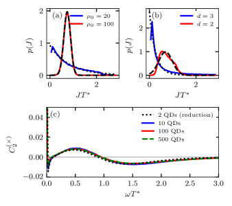
Figure 1: (a) Distribution $p(\overline{J}_{i})$ for an exponential distance dependency $J(r_{ij})\propto\exp(-r_{ij}/\rho_{0})$ for two different values of $\rho_{0}$ measured in $\mathrm{nm}$. (b) Power law $J(r_{ij})\propto r_{ij}^{-d}$ with $d=2$ or $d=3$. The curves can be approximated by an exponential function (dotted lines) or a Gaussian function (dashed lines). (c) The cross-correlation spectra for ensembles of different sizes are compared to a reduced two-QD model. For the QD ensembles the distance-dependent coupling constant, Eq. (28) with $\rho_{0}=20\,\mathrm{nm}$, and for the reduced two-QD model the exponential distribution $p(J)$ is used.

By inspecting the EOM, the effect of all other electron spins onto the electron spin of the i-th QD,

$$\vec{b}_{J}^{(i)} = \sum_{j}J_{ij}\vec{s}^{(j)},$$ (29)

is identified as an additional noise source. Its expectation value vanishes in the high-temperature limit but its variance

$$\langle(\vec{b}_{J}^{(i)})^{2}\rangle = \sum_{j}J^{2}_{ij}\langle(\vec{s}^{(j)})^{2}\rangle=(\bar{J}_{i})^{2}\langle S^{2}\rangle$$ (30)

is finite for coupling constants $J_{ij}$ that decay fast enough with the distance $r_{ij}$ between the QDs. In the last step, we defined the quadratically averaged coupling constant for each QD $i$:

$$\overline{J}_{i} = \sqrt{\sum_{j}J^{2}_{ij}},$$ (31)

which is possible, since all spins have the same length $(\vec{s}^{(j)})^{2}=S^{2}$. In our simulations, we choose $\alpha$ in Eq. (28) such that the averaged fluctuation strength

$$\bar{J} = \frac{1}{N_{\rm QD}}\sum_{i=1}^{N_{\rm QD}}\overline{J}_{i}=\frac{1}{T^{*}}$$ (32)

is fulfilled. This is a reasonable value since experimental data on samples with interacting QDs [52] suggests that the dephasing via the QD interaction is of the same order of magnitude as the dephasing by the local Overhauser field.

In the ensemble, $\overline{J}_{i}$ differs for the individual QDs $i$. Therefore, we not only calculate the average $\bar{J}$ but also compile the histogram of all values $\overline{J}_{i}$ and average over many different realizations of the randomly generated QD ensembles to obtain a probability distribution $p(J)$ for finding the coupling strength $J=\overline{J}_{i}$ in the i-th QD.

Assuming that we have a microscopic model that provides the coupling constant $J_{ij}=J(\vec{R}_{i},\vec{R}_{j},\rho_{0})$ for each QD pair of the original ensemble, we calculate the effective coupling constant $\bar{J}_{i}$ according to Eq. (31) for each QD of a random configuration $\{\vec{R}_{i}\}$ to obtain the distribution $p(\bar{J}_{i})$ of the effective coupling constants for a given characteristic length scale $\rho_{0}$. This distribution $p(\bar{J}_{i})$ is presented for two different values of $\rho_{0}$ in Fig. 1(a) using the exponential form of Eq. (28). While $p(\bar{J}_{i})$ can be well approximated by an exponential distribution for a short-range interaction $\rho_{0}=20\,\mathrm{nm}$, $p(\bar{J}_{i})$ approaches a Gaussian for a long-range interaction, $\rho_{0}=100\,\mathrm{nm}$, due to the central-limit theorem which is displayed as dashed line.

We added the distribution $p(J)$ for a power law dependency

$$J(r_{ij})=\alpha r_{ij}^{-d},$$ (33)

with the prefactor $\alpha$ and exponent $d$ as Fig. 1(b). We observe the same generic behavior with a short-range interaction for $d=3$ and a long-range interaction for $d=2$. Such a power law distance dependency could occur for an RKKY mediated effective coupling when some of the donator charges populate the conduction band of the wetting layer.

To measure the cross-correlation function in the ensemble, we divide the QDs into two classes and replace $S_{z}^{(i)}$ in Eq. (23) by the averaged spin of the respective class. We compare the cross-correlation spectra for ensembles of different sizes in the absence of an external magnetic field. In Fig. 1(c) the cross-correlation spectra for different numbers of QDs from $N_{QD}=10$ to $N_{QD}=500$ are presented as colored lines. We postpone the physical interpretation of the curves to latter and only notice that the spectra for different ensemble sizes coincide, which is attributed to the short-range nature of the interaction between the QDs. In the high-temperature limit long-range correlations between the QDs are absent and the consideration of a small cluster is sufficient [58].

For a further reduction of the system size we note that the influence of the other QDs onto the electron spin dynamics is encoded in a single effective magnetic field, $\vec{b}_{J}^{(i)}$ introduced in Eq. (29). Since the electron spin dephasing in a QD is governed by the overall fluctuations of $\vec{b}_{J}^{(i)}$, we can efficiently simulate the effect of a large number of QDs onto the spin dynamics by replacing the sum over all other QDs by a single additional QD employing an effective coupling constant $J=\overline{J}_{i}$. The system reduces to an effective two-QD problem where the two QDs represent their respective class, however, we ignore higher-order inter-QD interactions. In order to mimic the randomness of the coupling constants $p(\overline{J}_{i})$ in the ensemble of QDs, we simulate many such coupled QD pairs by drawing the effective coupling constant $J$ from a distribution $p(J)$ for each classical configuration, such that the distribution of $\vec{b}_{J}^{(i)}$ remains unchanged.

We added the cross-correlation spectrum for the reduced two-QD model as a dotted black line to Fig. 1(c), where we use the exponential distribution $p(J)$. The agreement between the full simulation of a random array of QDs and the averaging over a distribution of many effective two-QD systems is remarkable. The reduced two-QD model reproduces the ensemble behavior with only very small deviations even for an average interaction strength $\bar{J}=1/T^{*}$ that is comparable to the Overhauser field fluctuation scale. In the absence of an external magnetic field, we find increasing deviations in the low-frequency part of the spectra once $\overline{J}_{i}$ significantly exceeds the Overhauser field strength (not shown here): when a single effective inter-QD interaction starts to dominate the electron spin correlations, a larger amount of QDs must be considered in order to capture the correct physics.

V.2 Auto- and cross-correlation spectrum in box-model limit

To explore the generic behavior of the system we study the auto and cross-correlation spectrum of two interacting QDs, which either represent a reduced ensemble, see Sec. V.1, or a QD molecule. We stick to the box-model approximation, i. e. $A_{k}^{(i)}=A_{0}$, restrict ourselves to $N_{i}=100$ nuclear spins of length $I=1/2$ which enables the comparison to an exact quantum mechanical approach (QMA). $\vec{I}_{\mathrm{tot}}^{(i)}=\sum_{k}\vec{I}_{k}^{(i)}$ can be replaced in Eq. (2) and the commutator relation $[(I_{\mathrm{tot}}^{(i)})^{2},H]=0$ holds. The Hamiltonian becomes block diagonal in the subspaces of fixed quantum numbers $\{I_{\mathrm{tot}}^{(i)}\}$, which reduces the complexity of the problem considerably [74] and larger values of $N_{i}$ become accessable. In order to relate the SCA and QMA the rescaled coupling constant $J^{\prime}=\sqrt{3/(4\braket{S^{2}})}J$ is used where $\braket{S^{2}}=1/4$ in the SCA and $\braket{S^{2}}=3/4$ in the QMA.

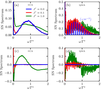
Figure 2: Comparison of the SCA (left panels) and QMA (right panels) for fixed $J^{\prime}$ measured in units of $1/T^{*}$. The upper panels, (a) and (b), show the autocorrelation spectrum, the lower panels, (c) and (d), depict the related cross-correlation spectrum. For a better presentation, the amplitude of the blue curve in panel (b) is reduced by the factor $10^{-1}$.

In a first step, we focus on the comparison of the autocorrelation spectra obtained by the SCA and the QMA which are presented in the upper panels of Figs. 2 and 3 respectively. In Fig. 2(a) the autocorrelation spectrum resulting from the SCA is depicted for various values of the inter-QD interaction strength $J^{\prime}$. Without interactions between the QDs ($J^{\prime}=0$), the total angular momentum $\vec{F}^{(i)}=\sum_{k}\vec{I}_{k}^{(i)}+\vec{S}^{(i)}$ is conserved for each QD and the autocorrelation spectrum coincides with the Frozen-Overhauser field solution of a single QD [29]. In this case, the correlation spectrum consists of a delta-peak at $\omega=0$, which corresponds to the non-decaying part of $C_{2}(t\rightarrow\infty)$, and a broader contribution from the Gaussian Overhauser field fluctuations with location and width governed by $1/T^{*}$. While the Overhauser field contributions are continuous in the SCA, they have a Dirac-comb substructure in the QMA, see Fig. 2(b), that reflects the transitions between the equidistant energy levels for a finite number of quantum mechanical states. In the box-model approximation, the quantum mechanical energy levels have a separation of $A_{0}\propto 1/\sqrt{N_{i}}$, which recovers the continuous spectrum for $N_{i}\rightarrow\infty$.

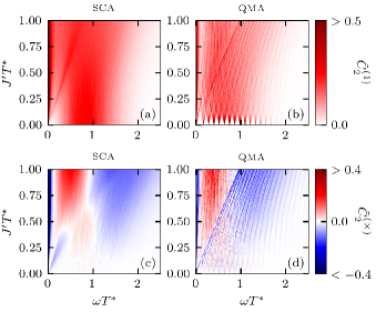
Figure 3: Comparison of the SCA and QMA. The upper panels, (a) and (b), show the autocorrelation spectrum, and the lower panels, (c) and (d), depict the cross-correlation spectrum as a function of the frequency $\omega$ and interaction strength $J^{\prime}$. The left panels, (a) and (c), correspond to the SCA and the right panels, (b) and (d), belong to the QMA. The magnitude of the correlation function is color coded according to the legends on the right-hand side.

At finite inter-QD interaction strength ($J\neq 0$), the conservation of the total spin $\vec{F}^{(i)}$ in each individual QD is lifted and only $\vec{F}_{\mathrm{tot}}=\sum_{i}\vec{F}^{(i)}$ remains conserved. As a consequence the sharp lines in the quantum mechanical autocorrelation spectrum fan out and, except for some noise, the discrete quantum mechanical spectrum resembles the continuous semiclassical spectrum for $N_{i}=100$ spins already.

In order to illustrate the evolution with increasing inter-QD coupling strength $J^{\prime}$, we present the autocorrelation spectra as function of $\omega$ and $J^{\prime}$ in two-dimensional color plots in Fig. 3(a) and (b). A strong red color encodes a large positive value of correlation while a dark blue color corresponds to negative values of the correlation function, i.e. a strong anticorrelation. In the quantum mechanical results in Fig. 3(b), a broadening of the equidistant $\delta$-peaks for increasing $J^{\prime}$ is clearly visible which progresses towards the classical continuum. As common features of SCA and QMA we observe three relevant aspects: First, the zero-frequency $\delta$-peak is broadened in both approaches (Fig. 3(a) and (b)) since $\vec{F}^{(i)}$ and hence the Overhauser field is not conserved anymore and a long-term decay of $C_{2}(t)$ sets in. Secondly, the zero-frequency peak partially splits into an additional peak at $\omega=J^{\prime}$ due to the Heisenberg interaction between the QDs: There is a splitoff line starting at the origin and increasing linearly with $J^{\prime}$ in the $(\omega,J^{\prime})$ plane. Thirdly, as soon as $J^{\prime}$ becomes comparable to $1/T^{*}$, the peak related to the Overhauser-field fluctuations broadens, which implies that the inter-QD interaction enter as an additional dephasing source and supplement the Overhauser field fluctuations. In this simplified picture, the electron spins of adjacent QDs provide an additional source for the spin noise and act like additional spins in the nuclear spin bath. However, in contrast to the nuclear spins, which provide a nearly static contribution, the adjacent electron spin is fluctuating which results in a non Gaussian shape for $J^{\prime}=1/T^{*}$.

In a next step we examine the cross-correlation spectra obtained by SCA and QMA, that have been plotted below the autocorrelation spectra in Figs. 2 and 3. Without interaction, $J^{\prime}=0$, the cross-correlation spectrum is zero, since the individual QDs are decoupled. For $J^{\prime}>0$, a frequency dependent spectrum emerges whose positive and negative components have the same weights due to the sum rule, Eq. (27c). For $J^{\prime}T^{*}\ll 1$, a sharp zero-frequency peak is found, indicating a synchronization between the electron spins of different QDs at very long time scales. With growing $J^{\prime}$ this zero-frequency peak splits into three contributions: a $\delta$-peak with positive spectral weight at exactly $\omega=0$, a second peak close to $\omega=0$ with negative spectral weight and another peak with negative spectral weight at $\omega=J^{\prime}$. This behavior is observed in the SCA data in Fig. 3(c), as well as the corresponding QMA results in Fig. 3(d). As an additional feature in the cross-correlation spectrum the Overhauser field fluctuations, which are responsible for the broad peak around $1/T^{*}$ of the autocorrelation spectrum, are reflected by a positive cross-correlation for the smaller frequencies and a negative cross-correlation for larger frequencies. Note, when $J^{\prime}$ becomes comparable to $1/T^{*}$, some of the mentioned features might interfere destructively and are not solely visible anymore. The cross-correlation spectrum for the QMA maintains its discrete nature for $J^{\prime}>0$, as shown in Fig. 2(d) and Fig. 3(d). The envelope function, however, is similar to the semiclassical spectrum supporting the application of the SCA for large spin systems.

V.3 Frozen Overhauser field solution

To understand the origin of the different positive and negative components in the cross-correlation spectrum, shown in Fig. 3, we study a simplified and analytically solvable system. We exploit the separation of the time scales between the electron and nuclear spin dynamics and study the problem on a short time scale (up to 100 ns) where the nuclear spins can be considered as frozen. Thus, approximation errors for small frequencies, where the assumption is not valid, are expected. To that end we start with a Hamiltonian in the electronic subspace for two-QDs

$$H_{e}=\vec{S}^{(1)}\vec{b}^{(1)}+\vec{S}^{(2)}\vec{b}^{(2)}+J\vec{S}^{(1)}\cdot\vec{S}^{(2)}$$ (34)

that are subject to individual time-constant fields $\vec{b}^{(i)}=\vec{b}^{(i)}_{\mathrm{ext}}+\vec{b}_{N}^{(i)}$. Without loss of generality we choose the $z$ axis along the averaged field $\vec{\overline{b}}=(\vec{b}^{(1)}+\vec{b}^{(2)})/2$ and define the field deviating from the average $\Delta\vec{b}=(\vec{b}^{(1)}-\vec{b}^{(2)})/2$. Then the Hamiltonian of the electronic subspace reads

$$H_{e}=\overline{b}(S_{z}^{(1)}+S_{z}^{(2)})+\Delta\vec{b}(\vec{S}^{(1)}-\vec{S}^{(2)})+J\vec{S}^{(1)}\cdot\vec{S}^{(2)}$$

$$\approx\overline{b}(S_{z}^{(1)}+S_{z}^{(2)})+\Delta b_{z}(S_{z}^{(1)}-S_{z}^{(2)})+J\vec{S}^{(1)}\cdot\vec{S}^{(2)}\;,$$ (35)

where in the last step we neglect the transversal components of the deviating field. This approximation is justified for large magnetic fields. Details as well as a solution of the Hamiltonian (35) can be found in Appendix D. This model is exactly solvable and can be used to extract the autocorrelation spectra and cross-correlation spectra. For the longitudinal functions we obtain the result

$$\braket{S_{z}^{(1)}(t)S_{z}^{(1)}}= \frac{1}{4}+\frac{\alpha^{2}(1-\alpha^{2})}{2}(\cos(\omega_{\parallel}t)-1)$$ (36a)

$$\braket{S_{z}^{(1)}(t)S_{z}^{(2)}}= \frac{\alpha^{2}(1-\alpha^{2})}{2}(1-\cos(\omega_{\parallel}t))$$ (36b)

with the abbreviations

$$\alpha=\frac{1}{\sqrt{2}}\frac{x}{\sqrt{1+x^{2}-\sqrt{1+x^{2}}}}\;\mathrm{and}\;x=\frac{J}{2\Delta b_{z}}.$$ (37)

The Eqs. (36a) and (36b) comprise an oscillating term of frequency

$$\omega_{\parallel}=\sqrt{J^{2}+4\Delta b_{z}^{2}}$$ (38)

as well as a constant part. Correspondingly, the Fourier transformation contains a $\delta$-peak at $\omega=\omega_{\parallel}$ from the oscillatory part and a $\delta(\omega)$ term from the constant part. In accordance to the sum-rules (27a)-(27c), both peaks carry positive spectral weights in the auto-correlation function whereas the cross-correlation spectrum contains a positive and a negative peak of equal weight. Note the limit $\alpha\stackrel{{\scriptstyle J\ll\Delta b_{z}}}{{\rightarrow}}1$ , which guarantees vanishing cross-correlations for $J=0$.

The transversal correlation functions in $x$ direction yield

$$\braket{S_{x}^{(1)}(t)S_{x}^{(1)}}= \frac{\alpha^{2}}{8}\left(\cos(\omega_{\perp}^{++}t)+\cos(\omega_{\perp}^{-+}t)\right)$$

$$+\frac{1-\alpha^{2}}{8}\left(\cos(\omega_{\perp}^{+-}t)+\cos(\omega_{\perp}^{--}t)\right)$$ (39a)

$$\braket{S_{x}^{(1)}(t)S_{x}^{(2)}}= \frac{\sqrt{\alpha^{2}(1-\alpha^{2})}}{8}(-\cos(\omega_{\perp}^{++}t)-\cos(\omega_{\perp}^{-+}t)$$

$$+\cos(\omega_{\perp}^{+-}t)+\cos(\omega_{\perp}^{--}t)),$$ (39b)

and, due to the spin rotational symmetry around the $z$-axis, they are the same as those in $y$ direction. In the transversal case the four frequencies

$$\omega_{\perp}^{\pm+}=\overline{b}\pm\left(\frac{J}{2}+\sqrt{\frac{J^{2}}{4}+(\Delta b_{z})^{2}}\right)$$ (40a)

$$\omega_{\perp}^{\pm-}=\overline{b}\pm\left(\frac{J}{2}-\sqrt{\frac{J^{2}}{4}+(\Delta b_{z})^{2}}\right),$$ (40b)

centered around $\overline{b}$, occur.

The terms ”longitudinal” and ”transversal” are usually defined with respect to $\vec{b}_{\mathrm{ext}}$ and not with respect to $\vec{\overline{b}}$. For large $b_{\mathrm{ext}}\gg b_{N}$ this distinction becomes obsolete, however for small $b_{\mathrm{ext}}$ an averaging over an isotropic distribution of random field $\vec{b}_{N}^{(i)}$ is required leading to a mixing of correlation functions in $x$ and $z$ direction. In the case $b_{\mathrm{ext}}=0$, the field $\vec{\overline{b}}$ is isotropically distributed and the correlation functions of all spatial directions $x$, $y$ and $z$ mix with equal proportion. Therefore, longitudinal and transversal components are comprised in the spectra in Fig. 3.

The frequencies $\omega_{\perp}^{\pm\pm}$ build up the positive and negative cross-correlations around $1/T^{*}$. The longitudinal spectrum produces the negative cross-correlation at $\omega_{\parallel}\approx J^{\prime}$ and positive cross-correlations at $\omega=0$. The positive correlations at $\omega=0$ follow from the fact that the frozen Overhauser field approximation does not allow the full relaxation of the electronic spins, even in the presence of their interactions with each other. Only the strong anti-correlation at very small frequencies, visible in Fig 3, are absent within this simplification: The frozen Overhauser field approximation disregards the slow dynamics of the nuclear spins on long time-scales and small frequencies.

Indeed, the sharp $\delta$-peaks in the correlation spectra of the simplified model are broadened by the randomness of the hyperfine couplings leading the a continuous spectrum after the averaging as in Figs. 2 and 3.

V.4 Randomness of the coupling parameters

In Secs. V.1 and V.2 we established that the simulation of full QD ensemble with a larger number of $N_{QD}$ is equivalent to a coupled two-QD problem in the SCA supplemented with appropriate distribution function $p(J)$ with respect to the calculation of two-color cross-correlation functions.

The SCA allows studies of a large spin system beyond the simplified box model and facilitates the introduction of additional interactions without significantly increasing the computational effort. In the following we study a system of $N_{QD}=2$ QDs with $N_{i}=100$ nuclear spins each. It either represents a large QD ensemble or a QD molecule. For the nuclear spins we use a spin length $I=3/2$, which matches the spin length of Ga or As isotopes. The hyperfine couplings are proportional to the probability density of the electron at the location of the nucleus $A_{k}\propto|\psi(\vec{r}_{k})|^{2}$. Under the assumption of a flat 2-dimensional QD and a Gaussian wave function $\psi(\vec{r})\propto\exp(-r^{2}/(2L^{2}))$ with the characteristic QD length scale $L$, we obtain the probability distribution

$$p(A_{k})=\frac{L^{2}}{R^{2}}\frac{1}{A_{k}},$$ (41)

where $R>L$ is the cutoff radius defining the smallest hyperfine constant $A_{\mathrm{min}}$. Here, we choose the cut-off radius $R=2L$ and the maximum hyperfine constant $A_{\mathrm{max}}$ in such a way that Eq. (3) is fulfilled [34].

We use the exponential distribution for the inter-QD interaction, see Sec. V.1, with a mean value of $\overline{J}=1/T^{*}$ in accordance to Refs. [53, 52]. Therefore, we perform configuration averaging over individual realizations of $A_{k}^{(i)}$ as well as the effective coupling constant $J$ between two QDs [52].

In addition we include the effect of nuclear-quadrupolar interactions on the auto- and cross-correlation spectrum at low frequencies. We use uniformly distributed coupling constants $q\in[0,2\overline{q}]$ with the mean value $\overline{q}=0.015(T^{*})^{-1}$ and the easy axis $\vec{n}_{Q}$ uniformly distributed in a cone around $\vec{e}_{z}$ with apex angle $\theta_{\mathrm{max}}=1.19$ and a biaxiality $\eta=0.5$ as a set of nuclear-quadrupolar interaction parameters introduced in Refs. [13].

V.5 Effect of quduadrupolar interactions

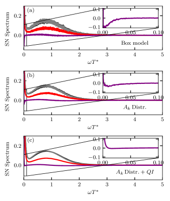
Figure 4: Comparison of the correlation spectra $\tilde{C}_{2}^{(1)}$ (red), $\tilde{C}_{2}^{(1+2)}$ (gray), $\tilde{C}_{2}^{(1)}+C_{2}^{(2)}$ (black) and $\tilde{C}_{2}^{(\times)}$ (violet) at ${B_{\mathrm{ext}}=0}$. Panel (a) uses the box-model approximation while in panels (b) and (c) the distribution in Eq. (41) is included. The quadrupolar interactions are omitted in panels (a) and (b), and are included in panel (c). The cross-correlation spectra at low-frequencies are enlarged in the insets.

In Fig. 4 we show various correlation spectra in the absence of an external magnetic field: the individual autocorrelation spectrum $\tilde{C}_{2}^{(1)}$ (red), the total autocorrelation spectrum $\tilde{C}_{2}^{(1+2)}$ (gray) and the cross-correlation spectrum $\tilde{C}_{2}^{(\times)}$ (violet). Fig. 4(a) depicts the results for the box-model approximation with homogeneous hyperfine coupling constants $A_{k}^{(i)}=A_{0}$ as a reference, in Fig. 4(b) we plot the data with an average over hyperfine coupling constants following the distribution, Eq. (41), and in Fig. 4(c) we add the nuclear-quadrupolar interaction term as well.

As both QDs are modeled with the same $T^{*}_{i}$, the individual autocorrelation functions of the electron spins are the same, i.e. $\tilde{C}_{2}^{(1)}=\tilde{C}_{2}^{(2)}$. The autocorrelation function of an individual electron spin displays two peaks at $\omega=0$ and $\omega=1/T^{*}$. Note, the inter-QD interaction only manifests in an additional broadening of both peaks, while the clear indications for inter-QD interactions, such as the peak at $\omega=J$, are smoothed out due to the randomness of $J$.

Figure 4(b) illustrates the effect of the distribution of hyperfine coupling constants. The Overhauser field is no longer proportional to the total angular momentum of the nuclear spins as in the box model and as a consequence a long term decay of the Overhauser field as well as the auto-correlation function $C_{2}^{(i)}(t)$ is possible. In the auto-correlation spectrum this reflects as a broadening of the zero-frequency peak, while higher frequency components are unchanged. The effect is intensified, when quadrupolar interactions are taken into account as well, see Fig. 4(c).

The summed $\tilde{C}_{2}^{(1)}+\tilde{C}_{2}^{(2)}$ and combined $\tilde{C}_{2}^{(1+2)}$ auto-correlation spectra are depicted in black and gray, respectively. While their general shape is rather similar to the auto-correlation spectrum of a single QD, the difference between the two defining the cross correlations contains additional information on the interaction between the QDs since it vanishes for QDs without inter-QD interaction.

In the box-model approximation, see Fig. 4(a), the cross-correlation spectrum contains a zero-frequency $\delta$-peak, just like the analytical solution for the FOA presented above. However, the anti-correlations at $\omega\propto J$ are not visible due to the $J$ averaging. The strong anti-correlations visible in the inset of Fig. 4(a), can be attributed to the slow dynamics of the nuclear spins.

In a system with an $A_{k}$ distribution, the broadening of the zero-frequency peak modifies the cross-correlation spectrum. The $\delta$-peak at $\omega=0$ is broadened and partially cancels out the adjacent anti-correlations at low frequencies, which as a result are strongly reduced as shown in the inset of Fig. 4(b).

This effect is even more pronounced when quadrupolar interactions are taken into account. Nuclear-electric quadrupolar-interactions originate from the strain induced by the self-assembled growth process. In the SCA they are reflected by time dependent fields acting on each nuclear spin independently. This introduces an additional disorder on the Overhauser field and, therefore, a broadening of the zero frequency peak. In Fig. 4(c) the effect of quadrupolar interactions for a realistic set of parameters [17, 13] is depicted. The zero-frequency peak is even more broadened. As a consequence the strong anti cross-correlations at low frequency vanish completely.

V.6 Effect of electron g-factor variation

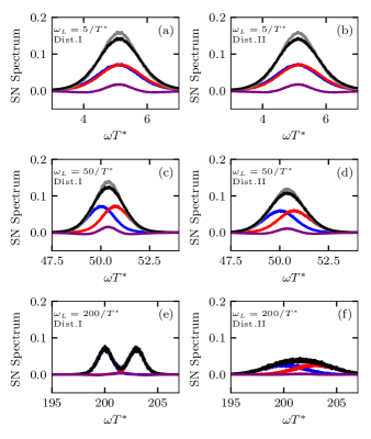
Figure 5: Comparison of the transversal correlation spectra $\tilde{C}_{2}^{(1)}$ (red), $\tilde{C}_{2}^{(2)}$ (blue), $\tilde{C}_{2}^{(1+2)}$ (gray), $\tilde{C}_{2}^{(1)}+\tilde{C}_{2}^{(2)}$ (black) and $\tilde{C}_{2}^{(\times)}$ (violet) for various external magnetic fields as well as g-factor distributions. The left panels correspond to distribution I, Eq. (42), the right panels relate to distribution II, Eq. (43). The external magnetic fields are $\omega_{L}=5/T^{*}$ ($B_{\mathrm{ext}}\approx 100\mathrm{mT}$) in panel (a) & (b), $\omega_{L}=100/T^{*}$ ($B_{\mathrm{ext}}=2\mathrm{T}$) in panel (c) & (d) and $\omega_{L}=200/T^{*}$ ($B_{\mathrm{ext}}=4\mathrm{T}$) in panel (e) & (f).

In this section we introduce a transverse external magnetic field acting on electron spins as well as nuclear spins. The electron spins precess in the external field with a Larmor frequency ${\omega_{L}=\mu_{B}g_{0}{B}_{\mathrm{ext}}}$, where $g_{0}=0.5$ is the typical effective $g$-factor of the electron in a InGaAs QD. For the nuclear spins we use the value $g_{k}^{(i)}\mu_{I}/g_{0}\mu_{B}\approx 1/800$ averaged over the different isotopes [61]. At large external magnetic fields, the spectral weight of the Gaussian shaped peak at $\omega\approx 1/T^{*}$ in the auto-correlation spectrum is shifted by this Larmor frequency. In the FOA this can be directly seen in the frequencies stated in Eq. (40a) and in Eq. (40b): They are shifted by $\overline{b}$. Consequently, effects relevant on long time-scales such as the distribution of hyperfine coupling constant or the nuclear quadrupolar interactions are suppressed. Only in spin-echo experiments [48, 75] described by fourth-order spin-spin correlation functions [19] a second dephasing time associated with these interactions occurs. Their effect is not observable in the second order correlations .

In a transversal field, however, the distribution of electron $g$ factors becomes relevant. Since the $g$ factor of an electron spin in a semiconductor is correlated with the excitation energy of the QD due to the Roth-Lax-Zwerdling relation, we assume that both QD subensembles have a different average $g$ factor [76, 52]. The optical selection of QDs used for the measurement of cross-correlation functions [42] is facilitated by the usage of probe lasers with different photon energies.

An additional variation of the $g$ factor for a fixed excitation energy is caused by local differences in a self-assembled QD ensemble. In order to study (i) the effect of a different g-factors in each subensemble as well as (ii) the $g$-factor variation within each subensemble we define the $g$-factor distribution I

$$g^{(1)} =g_{0}$$

$$g^{(2)} =1.015g_{0}$$ (42)

and $g$-factor distribution II

$$g^{(1)} \sim\mathcal{N}(g_{0},0.005)$$

$$g^{(2)} \sim\mathcal{N}(1.015g_{0},0.005)$$ (43)

where we use parameters extracted from literature [52, 59]. While for the distribution I the electrons 1 and 2 have different but fixed $g$ factors, the $g$ factor is drawn from a Gaussian distribution with a very small width [52] for the distribution II.

The impact of both distributions on the spectral functions is presented in Fig. 5 for different transverse external magnetic fields. The left panels belong to distribution I whereas the right panels use distribution II. Various correlation spectra at small magnetic fields of $\omega_{L}=5/T^{*}$ ($B_{\mathrm{ext}}\approx 100\mathrm{mT}$) applied in the $x$-direction are depicted in Figs. 5(a) and 5(b) using the color coding of Fig. 4 with an additional blue line for the individual auto-correlation function $\tilde{C}_{2}^{(2)}$ (that now differs from $\tilde{C}_{2}^{(1)}$). For this small field the $g$-factors distribution is rather irrelevant, since the energy scale $\Delta\omega=B_{\mathrm{ext}}\mu_{B}(g^{(1)}-g^{(2)})$ is small in comparison to the other energy scales of the system. Due to the transversal magnetic field the auto-correlation spectrum (red and blue line) has a Gaussian shape [29] and is centered around the Larmor frequency of the respective QD. Without inter-QD interaction, the width of the Gaussian is given by the Overhauser field fluctuations as well as the variation of $g$-factors. However, the latter effect is not relevant here which leaves $1/T^{*}$ as the only influence.

As the auto-correlation spectrum, the cross-correlation spectrum (purple line) is centered around the Larmor frequency $\omega_{L}$. It is positive in the center and is flanked by negative contributions at the wings. This behavior can be understood within the FOA. Relevant for the cross-correlation spectrum are the four frequencies in the Eqs. (40a) and (40b). While the two outer frequencies $\omega_{\perp}^{\pm+}$ have negative prefactors, the two inner frequencies $\omega_{\perp}^{\pm-}$ have a positive contribution to the cross-correlation spectrum. The sharp lines of the single configuration FOA analysis presented above are broadened due to the Overhauser-field fluctuations.

In a larger magnetic field, $\omega_{L}=50/T^{*}$ ($B_{\mathrm{ext}}\approx 1\mathrm{T}$), the splitting of the peak location due to the different $g$ factors is clearly visible in the auto-correlation functions of both QDs in Fig. 5(c). The cross-correlation function, however, retains its shape. Its amplitude is significantly reduced by the $g$ factor distribution II as can be seen in Fig. 5(d). The four lines obtained from the FOA, smear out due to the $g$-factor spreading and cancel each other.

For an even larger field, $\omega_{L}=200/T^{*}$ ($B_{\mathrm{ext}}\approx 4\mathrm{T}$), the auto-correlation spectra of the different QDs shown in Fig. 5(e) separate since the difference in the Larmor frequencies $\Delta\omega$ becomes significant. The cross-correlation strongly reduces for distribution I, since the prefactor $\alpha$ vanishes for $J/\Delta b\rightarrow 0$. By taking into account distribution II, the cross-correlation spectrum is almost completely washed out as depicted in Fig. 5(f).

In a transversal magnetic field, dephasing effects on long time scales such as caused by the quadrupolar interactions are suppressed since the cross-correlation spectrum is shifted to higher frequencies. The spectral features in the vicinity of the Larmor frequency, however, are suppressed in strong magnetic fields by a $g$-factor disorder leading to an attenuation of the cross-correlation spectrum. However, at small magnetic fields neither long time dephasing nor the $g$-factor dispersion attenuates the cross-correlation spectrum.

V.7 Longitudinal magnetic field

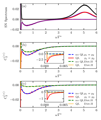
Figure 6: In panel (a) the correlation spectra $C_{2}^{(1)}$ (blue), $C_{2}^{(2)}$ (red), $C_{2}^{(1+2)}$ (gray), $C_{2}^{(1)}+C_{2}^{(2)}$ (black) and $C_{2}^{(\times)}$ (violet) are depicted for a longitudinal magnetic field of $\omega_{L}=5/T^{*}$. In the lower panels the cross-correlation spectrum $C_{2}^{(\times)}$ is depicted for the four combinations of: (i) quadrupolar interactions switched on and off and (ii) identical electron $g$-factors or distribution II, Eq. (43). Panel (b) presents $\omega_{L}=50/T^{*}$ and panel (c) $\omega_{L}=200/T^{*}$.

In this section, we present the results for the cross-correlation spectrum in a longitudinal external magnetic field, where both long- and short-time effects are apparently relevant. In Fig. 6(a) the correlation spectra in a weak longitudinal field of $\omega_{L}=5/T^{*}$ are depicted using the same color code as in the previous figures. We included the distribution of hyperfine coupling constants, the quadrupolar interactions and the $g$-factor distribution II in the dynamics.

For the auto-correlation spectra (red and blue), we observe a zero-frequency peak that is associated with the conserved spin projection along the external magnetic field axis in FOA, broadened due to the dephasing induced by quadrupolar interactions. In addition, some intermixing of the transversal spin components is visible in the peak centered around the Larmor frequency.

To understand the cross-correlation spectrum (violet) we again refer to the FOA results in Eq. (36b). It predicts a positive cross-correlation at $\omega=0$ and an anti-correlation at $\omega=\omega_{\parallel}$. For large $J$ we can approximate $\omega_{\parallel}\approx J$, accordingly the cross-correlations are sensitive to the distribution of coupling constants $p(J)$. Therefore, cross-correlation spin-noise spectroscopy in a longitudinal field provides the possibility to study the distribution of inter-QD couplings in an ensemble, an information that is not otherwise accessible.

We present the cross-correlation spectra for longitudinal fields $\omega_{L}=50/T^{*}$ in Fig. 6(b) and $\omega_{L}=200/T^{*}$ in Fig. 6(c) for the four combinations of (i) quadrupolar interactions included or not, and (ii) identical electron $g$-factors or distribution II. The low frequency behavior is enlarged in the insets. The positive cross-correlations predicted by the FOA, can be found as the $\delta$-peak at $\omega=0$. In addition, we find strong anti-correlations at small frequencies (orange) that we assign to the nuclear-quadrupolar interactions, that are absent in the FOA results, since the nuclear spins are considered frozen. The quadrupolar interactions, however, only plays a role at very low frequencies.

In contrast the distribution of $g$-factors does not change the shape of the cross-correlation spectrum, but lowers the amplitude. This attenuation effect is not as strong as in the transversal magnetic field, since no destructive interference between positive and negative lines occur and only enters via the prefactor $\alpha$ Eq. (37). At larger field of $\omega_{L}=200/T^{*}$ the effects of quadrupolar interactions and $g$-factor distribution are modified. The nuclear Zeeman term suppresses the effect of the quadrupolar interactions [15] which is indicated by a weakening of the peak caused by the quadrupolar interactions. In addition the attenuation effect of the $g$-factor distribution is enhanced strongly reducing the signal.

V.8 Connection to experiment

The auto-correlation spectrum $C_{2}^{(i)}$ corresponds to the noise power-spectrum that is experimentally [15] extensively studied and already well understood in terms of a single QD picture, where inter-QD interactions are neglected [29, 13]. In our framework we demonstrated that the auto-correlation spectrum qualitatively remains unchanged by the inter-QD interaction only the broadening of the peaks is modified. These modifications can be absorbed in a renormalization of $T^{*}$ translating into the parameters in a single-QD picture, so that all previous results can be embedded into the extension to interacting QDs.

Recently, the auto-correlation spectra $C_{2}^{(1)}$, $C_{2}^{(2)}$ and $C_{2}^{(1+2)}$ are measured for a QD ensemble at zero magnetic field to determine the homogeneous line widths [72]. Since the cross-correlation function $C_{2}^{(\times)}(t)$ is determined by the difference between the total two-color signal and the sum of the individual contributions according to Eq. (IV.2), $C_{2}^{(\times)}(t)$ could be extracted.

The experimental data in Ref. [72] qualitatively agrees with our results, as the cross-correlation spectrum is strongly attenuated at low frequencies by quadrupolar interactions and the hyperfine distribution – see Fig. 4(c). One has to bear in mind, however, that only 10% of the QDs were charged in the sample studied in Ref. [72], which strongly reduces spin-spin interactions between the QDs.

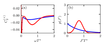
Figure 7: Effect of the distribution $p(J^{\prime})$ on the cross-correlation spectrum in a longitudinal magnetic field of $\omega_{L}=5/T^{*}$. Panel (a) depicts the cross-correlation spectrum while panel (b) shows the associated distribution function $p(J^{\prime})$. The red curves belong to a Gaussian distribution with mean value $\overline{J}=1/T^{*}$ and standard deviation $\sigma=0.3/T^{*}$. The blue curves belong to an exponential distribution with $\overline{J}=1/T^{*}$.

As a consequence of our investigation we propose to measure the cross-correlation spectrum at a finite but low external magnetic field, where additional dephasing by the $g$-factor distribution is negligible. The strongest cross-correlation signal is expected for a transversal magnetic field, for which the quadrupolar interaction is suppressed.

¿From the longitudinal cross-correlation spectrum, additional information about the distribution of the interaction strength $J$ can be obtained, even though the signal strength is expected to be lower than in the transverse case. We present the cross-correlation spectrum for two different distribution function $p(J)$ in Fig. 7. The cross-correlation function obtained from a Gaussian distribution $p(J)$ and depicted in red significantly deviated from the one calculated with a exponential distribution plotted in blue. This way, one can extract additional details about the microscopical origin and the characteristic length scale of the inter-QD interactions.

VI Conclusion

We studied the spin-noise spectrum for an ensemble of singly charged QDs whose resident electron spins interact via a Heisenberg type interaction. To this end, we employed a SCA that allows for the description of coupled spin systems comprising a larger number of spins than e.g. would be manageable in straight forward quantum mechanical calculations. The approach is based on the introduction of the classical Hamilton function derived from an arbitrary quantum mechanical Hamiltonian via spin-coherent states. This procedure accounts for a correct description of terms in the Hamiltonian that are quadratic in the spin operators as it occurs in the case of nuclear quadrupolar interactions.

For two-color spectroscopy we were able to map the ensemble problem onto a pair of coupled QDs augmented with a coupling constant distribution. Studying the mapped system, we find features in the spin-noise spectrum related to the inter-QD interaction. In the absence of an external magnetic field, the hyperfine interaction and the nuclear quadrupolar interactions conceal a potential effect of an inter-QD interaction on the correlation spectra.

The application of an external magnetic field either transverse or longitudinal to the measurement axis allows for the separation of the inter-QD interaction from other contributions in the cross-correlation spectra. In case of a transversal external magnetic field, the field strength has to be adjusted in an intermediate region in order to achieve a significant shift of the Larmor frequencies for the two electron spins due to their slightly differing $g$ factors, but not to suppress the effect of inter-QD interaction completely. However, the longitudinal field may provide easier access. Here, the contribution of the inter-QD interaction in the cross-correlation spectrum is strongly pronounced over a broad range of the magnetic field strengths. The shape of the cross-correlation spectrum can even provide information on the distribution of the coupling strength and thereby hint on the unclear physical origin of the interaction. Experimental cross correlation data could be an interesting step towards further understanding to the interaction between electron spins in QD ensembles.

Appendix A Derivation of the SCA from a path integral formulation

We start with the propagator

$$K(\{\vec{s}_{j,f}\},\{\vec{s}_{j,i}\},t) =\bra{\{\vec{s}_{j,f}\}}e^{-iHt}\ket{\{\vec{s}_{j,i}\}}$$ (44)

which provides the transition amplitude from the initial state $\ket{\{\vec{s}_{j,i}\}}$ at time $0$ to the final state $\ket{\{\vec{s}_{j,f}\}}$ at time $t$. $\{\vec{s}_{j,f}\}$ denotes the set of all electron and nuclear spins of the ensemble.

We decompose the time evolution operator into small time intervals $\Delta t=t/N$

$$K(\{\vec{s}_{j,f}\},\{\vec{s}_{j,i}\},t)=\lim\limits_{N\rightarrow\infty}\bra{\{\vec{s}_{j,f}\}}\prod_{n=0}^{N-1}e^{-iH\Delta t}\ket{\{\vec{s}_{j,i}\}}\;.$$ (45)

Now we can insert the completeness relation (8) between all infinitesimal time evolution operators to get infinitesimal transition amplitudes

$$K(\{\vec{s}_{j,f}\},\{\vec{s}_{j,i}\},t)=\lim\limits_{N\rightarrow\infty}\int\prod_{n=1}^{N-1}d\mu(\{\vec{s}_{j,n})$$

$$\times\prod_{n=0}^{N-1}\bra{\{\vec{s}_{j,n+1}\}}e^{-iH\Delta t}\ket{\{\vec{s}_{j,n}\}}$$ (46)

with $\ket{\{\vec{s}_{j,0}\}}=\ket{\{\vec{s}_{j,i}\}}$ and $\ket{\{\vec{s}_{j,N}\}}=\ket{\{\vec{s}_{j,f}\}}$.

Next, we estimate the transition amplitude for very small time steps, $\bra{\{\vec{s}_{j,n+1}\}}e^{-iH\Delta t}\ket{\{\vec{s}_{j,n}\}}$. Using the Taylor expansion of the exponential up to linear order, and including the difference between $\langle\{\vec{s}_{j,n+1}\}\ket{\{\vec{s}_{j,n}\}}$ and $1=\langle\{\vec{s}_{j,n}\}\ket{\{\vec{s}_{j,n}\}}$, we obtain

$$\bra{\{\vec{s}_{j,n+1}\}}e^{-iH\Delta t}\ket{\{\vec{s}_{j,n}\}} = \langle\{\vec{s}_{j,n+1}\}\ket{\{\vec{s}_{j,n}\}}-i\Delta t\bra{\{\vec{s}_{j,n+1}\}}H\ket{\{\vec{s}_{j,n}\}}+O(\Delta t^{2})$$ (47)

$$= e^{-i\left(i\bra{\{\vec{s}_{j,n}\}}\frac{d}{dt}\ket{\{\vec{s}_{j,n}\}}+\bra{\{\vec{s}_{j,n}\}}H\ket{\{\vec{s}_{j,n}\}}\right)\Delta t}+O(\Delta t^{2}).$$

Making use of the fact that $\Delta t$ is arbitrary small and inserting the exponential into the Eq. (46) yields

$$K(\{\vec{s}_{j,f}\},\{\vec{s}_{j,i}\},t) = \lim\limits_{N\rightarrow\infty}\int\prod_{n=1}^{N-1}d\mu(\{\vec{s}_{j,n}\})e^{-i\sum_{n=0}^{N-1}\left(i\bra{\{\vec{s}_{j,n}\}}\frac{d}{dt}\ket{\{\vec{s}_{j,n}\}}+\bra{\{\vec{s}_{j,n}\}}H\ket{\{\vec{s}_{j,n}\}}\right)\Delta t}$$

At this point the transition amplitude can be identified as a path integral that can be comprehensively written as

$$K(\{\vec{s}_{j,f}\},\{\vec{s}_{j,i}\},t) =\int\mathcal{D}[\{\vec{s}_{j}\}]\;e^{iS[\{\vec{s}_{j}\},\{\partial_{t}\vec{s}_{j}\}]}$$ (48)

with the action

$$S[\{\vec{s}_{j}\},\{\partial_{t}\vec{s}_{j}\}]=\int\left(i\bra{\{\vec{s}_{j}\}}\frac{d}{dt}\ket{\{\vec{s}_{j}\}}-\bra{\{\vec{s}_{j}\}}H\ket{\{\vec{s}_{j}\}}\right)dt,$$ (49)

and the integration measure

$$\mathcal{D}[\{\vec{s}_{j}\}]=\lim\limits_{N\rightarrow\infty}\prod_{n=1}^{N-1}d\mu(\{\vec{s}_{j,n}\})\;.$$ (50)

This path integral formulation of the transition amplitude was used to derived the SCA using a saddle-point approximation leading to the Euler-Lagrange Eq. (13) for the coherent state using the action $S$.

Appendix B Quadrupolar Hamiltonian

The quadrupolar interaction acting on a single nuclear spin is quantum mechanically described by the Hamiltonian

$$H_{Q}=q\left[\left(\vec{I}\cdot\vec{n}\right)^{2}+\frac{\eta}{3}\left(\left(\vec{I}\cdot\vec{n}_{x}\right)^{2}-\left(\vec{I}\cdot\vec{n}_{y}\right)^{2}\right)\right].$$ (51)

In the following, our aim is to derive the semiclassical EOM for the classical nuclear spin from this Hamiltonian.

First, we have to calculate the classical Hamilton function $\tilde{H}(\vec{i})$ with the classical nuclear vector $\vec{i}$ entering the action S defined in Eq. (49). Since the quadrupolar Hamiltonian consists of three similar terms, we evaluate a term of the general form

$$\bra{\vec{i}}(\vec{I}\cdot\vec{m})^{2}\ket{\vec{i}} =\bra{I,I}e^{i(\vec{\theta}\times\vec{n}_{0})\cdot\vec{I}}(\vec{I}\cdot\vec{m})^{2}e^{-i(\vec{\theta}\times\vec{n}_{0})\cdot\vec{I}}\ket{I,I}$$

$$=\bra{I,I}(\vec{I}\cdot\tilde{\vec{m}})^{2}\ket{I,I}\;.$$ (52)

¿From the first to the second line, we insert the rotation that relates the spin-coherent state $\ket{\vec{i}}$ to the spin state with maximum quantum spin number in the $z$ component $\ket{I,I}$. These two unitary operators are used to rotated the orientation vector $\vec{m}$ to $\tilde{\vec{m}}$, so that the total matrix element remains invariant.

In a next step, we insert the spin operator

$$\vec{I}=\left(I^{x},I^{y},I^{z}\right)^{T}=\left(\frac{1}{2}\left(I^{+}+I^{-}\right),\;\frac{1}{2i}\left(I^{+}-I^{-}\right),\;I^{z}\right)^{T}$$ (53)

leading to

$$\bra{\vec{i}}(\hat{\vec{I}}\cdot\vec{m})^{2}\ket{\vec{i}} =\bra{I,I}\frac{1}{4}\left[(\tilde{m}^{x})^{2}+(\tilde{m}^{y})^{2}\right]I^{+}I^{-}$$

$$+(\tilde{m}^{z})^{2}(I^{z})^{2}\ket{I,I}\;.$$ (54)

We insert $\hat{I}^{+}\hat{I}^{-}\ket{I,I}=2I\ket{I,I}$ and $(\hat{I}^{z})^{2}\ket{I,I}=I^{2}\ket{I,I}$ and obtain

$$\bra{\vec{i}}(\hat{\vec{I}}\cdot\vec{m})^{2}\ket{\vec{i}} =\frac{I}{2}+\left(1-\frac{1}{2I}\right)(\tilde{m}^{z})^{2}I^{2}$$

$$=\frac{I}{2}+\left(1-\frac{1}{2I}\right)\left(\tilde{\vec{m}}\cdot\vec{e}^{z}I\right)^{2}.$$ (55)

After rotating back into the original coordinate space, the final result reads

$$\bra{\vec{i}}(\hat{\vec{I}}\cdot\vec{m})^{2}\ket{\vec{i}} =\frac{I}{2}+\left(1-\frac{1}{2I}\right)\left(\vec{i}\cdot\vec{m}\right)^{2}\;.$$ (56)

When we apply this relation to the three terms of the quadrupolar Hamiltonian in Eq. (51), the classical Hamilton function entering the action $S$, derived from the quantum mechanical operator $\hat{H}_{Q}$, is given by

$$\tilde{H}_{Q}= q\left\{\frac{I}{2}+\left(1-\frac{1}{2I}\right)\left(\vec{i}\cdot\vec{n}\right)^{2}\right.$$

$$\left.+\frac{\eta}{3}\left(1-\frac{1}{2I}\right)\left[\left(\vec{i}\cdot\vec{n}_{x}\right)^{2}-\left(\vec{i}\cdot\vec{n}_{y}\right)^{2}\right]\right\}\;.$$ (57)

$\tilde{H}_{Q}$ has been used to obtain the quadrupolar field in Eq. (16) by applying the general EOM stated in Eq. (13).

Appendix C Auto-correlation function in semiclassical form

Let us transform the auto-correlation function

$$C_{2}(t)=\left<S^{z}(0)S^{z}(t)\right>.$$ (58)

into a suitable form for the SCA. As a demonstration, we start by the calculation of $C_{2}$ for a single isolated spin $1/2$ and only then generalize the results to more complex systems. The most general time-dependent Hamiltonian for a single spin $1/2$ has four degrees of freedom and can be parameterized by $H(t)=\vec{B}(t)\cdot\vec{S}+E_{0}(t)$, whereby $E_{0}(t)$ solely creates a global phase factor that does not have any impact in our case.

The time evolution is governed by the operator

$$U(t) =\mathcal{T}\exp\left(-i\int_{0}^{t}H(t)dt\right)$$

$$=e^{i\varphi(t)}\exp\left(-i\,\vec{\alpha}(t)\cdot\vec{S}\right)=e^{i\varphi(t)}R_{\vec{\alpha}(t)},$$ (59)

with the time-ordering operator $\mathcal{T}$ and the global phase $e^{i\varphi(t)}$. Since $U(t)$ is an element of the rotation group SU(2), we have replaced the time-ordered integral in the second line of Eq. (59) by a rotation along a specific axis $\vec{\alpha}\in\mathbb{R}^{3}$, whose explicit calculation shall be postponed for the moment. We use the latter representation of $U(t)$ to calculate the correlator $C_{2}$ with respect to an initial spin-coherent state $\ket{\vec{s}_{0}}$

$$C_{2} =\bra{\vec{s}_{0}}S^{z}(0)S^{z}(t)\ket{\vec{s}_{0}}$$ (60)

$$=\bra{\vec{s}_{0}}(\vec{e}_{z}\cdot\vec{S})R_{-\vec{\alpha}(t)}(\vec{e}_{z}\cdot\vec{S})R_{\vec{\alpha}(t)}\ket{\vec{s}_{0}}.$$ (61)

In a next step we make use of the relation

$$R_{-\vec{\alpha}}(\vec{e}_{z}\cdot\vec{S})R_{\vec{\alpha}} =(\tilde{R}_{-\vec{\alpha}}\vec{e}_{z})\cdot\vec{S}\;,$$ (62)

that translates a rotation $R_{\vec{\alpha}}$ of the SU(2) to a $3\times 3$ rotation matrix $\tilde{R}_{-\vec{\alpha}}=\exp(-\left[\vec{\alpha}\right]_{x})$ of the SO(3), using the cross-product matrix $\left[\vec{\alpha}\right]_{x}$. This yields

$$C_{2} =\bra{\vec{s}_{0}}(\vec{n}_{z}(0)\cdot\vec{S})(\vec{n}_{z}(t)\cdot\vec{S})\ket{\vec{s}_{0}},$$ (63)

with the rotated $z$ axis $\vec{n}_{z}(t)=\tilde{R}_{-\vec{\alpha}(t)}\vec{e}_{z}$.

Finally, the auto-correlation function, Eq. (63), is converted to a fully classical form. To this end, standard spin $1/2$ algebra, i.e. the relation $S^{\alpha}S^{\beta}=(1/4)\delta_{\alpha\beta}+(i/2)\sum_{\gamma}\epsilon_{\alpha\beta\gamma}S^{\gamma}$, and the relation $\bra{\vec{s}_{0}}\vec{S}\ket{\vec{s}_{0}}=\vec{s}_{0}$ are exploited, such that the auto-correlation function for the single spin 1/2 becomes

$$C_{2} =\frac{1}{4}\vec{n}_{z}(0)\cdot\vec{n}_{z}(t)+\frac{i}{2}(\vec{n}_{z}(0)\times\vec{n}_{z}(t))\cdot\vec{s}_{0}$$ (64)

for a fixed initial coherent state $\ket{\vec{s}_{0}}$ and the fixed time $t$.

This leaves us with the calculation of the rotation matrix as function of time. By identifying $\vec{B}(t)$ in the Hamiltonian of the single spin 1/2 with the effective field $\vec{b}_{\mathrm{eff}}(t)=\frac{\partial\tilde{H}(\vec{s})}{\partial\vec{s}}$, we can interpret Eq. (64) as a recipe for evaluation of $C_{2}$ in a more complex system described by the Hamilton function $\tilde{H}(\vec{s})$ in the semiclassical limit.

In a last step, we present an efficient way to compute the rotation matrix $\tilde{R}_{\vec{\alpha}}$ within the SCA. Instead of calculating the rotation matrix directly, we use its quaternionic representation [47], which is more compact and numerically stable. Unit quaterions are isomorphic with the group SU(2), which becomes particular clear, considering that the basic quaternions $\{1,i,k,l\}$ and the Pauli matrices $\{\mathbb{1},i\sigma_{1},i\sigma_{2},i\sigma_{3}\}$ share the same algebra. However, unit quaternions can also be used to represent the SO(3) rotation group due to the two-to-one homomorphism of the SU(2) onto the SO(3). A SO(3) rotation $\tilde{R}_{\vec{\alpha}}$ can be represented by the unit quaternion

$$Q(\vec{\alpha})=\cos(\alpha/2)+\frac{\vec{\alpha}}{\alpha}\cdot\vec{j}\sin(\alpha/2)\;,$$ (65)

with the basic quaternions $\vec{j}=(i,k,l)^{T}$. As the SO(3) is covered twice in the SU(2), the quaterions $Q$ and $-Q$ represent the same SO(3) rotation. It can be shown that the desired rotation can be applied to a vector with the quaternion multiplication and its inverse

$$\vec{j}\vec{n}(t)=Q(\vec{j}\vec{n}(0))Q^{-1}\;.$$ (66)

Consequently two consecutive rotations are combined by the quaternion multiplication $Q=Q_{1}Q_{2}$.

We can derive a simple EOM for $Q$ by applying an infinitesimal rotation $Q^{\prime}\approx 1+\vec{b}_{\mathrm{eff}}\vec{j}dt$ to $Q$ with the quaternion multiplication

$$\frac{Q^{\prime}Q-Q}{dt} =-\vec{b}_{\mathrm{eff}}\cdot\vec{v}+(q\vec{b}_{\mathrm{eff}}+\vec{b}_{\mathrm{eff}}\times\vec{v})\cdot\vec{j},$$ (67)

where we divide the rotation $Q=q+\vec{v}\vec{j}$ into scalar part $q\in\mathbb{R}$ and a vector part $v\in\mathbb{R}^{3}$. In conclusion we get the EOM for the quaternionic representation of the rotation matrix

$$\frac{dq}{dt} =-\vec{b}_{\mathrm{eff}}\cdot\vec{v}\;,$$ (68)

$$\frac{d\vec{v}}{dt} =q\vec{b}_{\mathrm{eff}}+\vec{b}_{\mathrm{eff}}\times\vec{v}\;,$$ (69)

which can be solved along-side the Eqs. (14a) and (14b).

Appendix D FOA - approximation and solution

We start with the Hamiltonian

$$H_{e}=\overline{b}(S_{z}^{(1)}+S_{z}^{(2)})+\Delta\vec{b}(\vec{S}^{(1)}-\vec{S}^{(2)})+J\vec{S}^{(1)}\cdot\vec{S}^{(2)}\;.$$ (70)

Using the operator $U=\exp(-ib(S_{z}^{(1)}+S_{z}^{(2)}))$, we transform into the rotating frame of $\vec{\overline{b}}$

$$H^{\prime} =\Delta\vec{b}(t)(S_{z}^{(1)}-S_{z}^{(2)})+J\vec{S}^{(1)}\cdot\vec{S}^{(2)}$$ (71)

$$\approx\Delta b_{z}(S_{z}^{(1)}-S_{z}^{(2)})+J\vec{S}^{(1)}\cdot\vec{S}^{(2)}\;,$$ (72)

where $\overline{b}$ vanishes and $\Delta\vec{b}(t)$ obtains a dependence on time. The time dependent deviational field $\Delta\vec{b}(t)=\Delta b_{z}\vec{e}_{z}+\Delta\vec{b}_{\perp}(t)$ can be split into a time-constant part along the $z$ axis and oscillating terms perpendicular to the $z$ direction. For $b_{ext}\gg b_{n}$, it is well justified to omit $\Delta\vec{b}_{\perp}(t)$ due to fast oscillating contributions. After omitting $\Delta\vec{b}_{\perp}(t)$ we rotate back out of the rotating frame and obtain

$$H_{e}\approx b(S_{z}^{(1)}+S_{z}^{(2)})+\Delta b_{z}(S_{z}^{(1)}-S_{z}^{(2)})+J\vec{S}^{(1)}\cdot\vec{S}^{(2)}.$$ (73)

This Hamiltonian commutes with $S_{z}=S_{z}^{(1)}+S_{z}^{(2)}$ and has the four eigenenergies

$$\epsilon_{1,2}=\frac{J}{4}\pm b;\hskip 28.45274pt\epsilon_{3,4}=-\frac{J}{4}\pm\sqrt{\frac{J^{2}}{4}+(\Delta b_{z})^{2}}.$$ (74)

The related eigenstates read

$$\ket{\epsilon_{1,2}} =\Ket{\pm\frac{1}{2},\pm\frac{1}{2}}$$ (75a)

$$\ket{\epsilon_{3,4}} =\alpha\Ket{\pm\frac{1}{2},\mp\frac{1}{2}}\pm\sqrt{1-\alpha^{2}}\Ket{\mp\frac{1}{2},\pm\frac{1}{2}}$$ (75b)

with the abbreviation

$$\alpha=\frac{1}{\sqrt{2}}\frac{x}{\sqrt{1+x^{2}-\sqrt{1+x^{2}}}}\;\mathrm{and}\;x=\frac{J}{2\Delta b_{z}},$$ (76)

(Limits: $\lim_{x\rightarrow 0}\alpha=1$ and $\lim_{x\rightarrow\infty}\alpha=\frac{1}{\sqrt{2}}$.) which can be used to calculate arbitrary spin-spin correlators within this approximation.

References

- Hanson et al. [2007] R. Hanson, L. P. Kouwenhoven, J. R. Petta, S. Tarucha, and L. M. K. Vandersypen, Spins in few-electron quantum dots, Rev. Mod. Phys. 79, 1217 (2007).
- Burkard et al. [2000] G. Burkard, H.-A. Engel, and D. Loss, Spintronics and quantum dots for quantum computing and quantum communication, Fortschritte der Physik 48, 965 (2000).
- Atatüre et al. [2006] M. Atatüre, J. Dreiser, A. Badolato, A. Högele, K. Karrai, and A. Imamoglu, Quantum-dot spin-state preparation with near-unity fidelity, Science 312, 551 (2006).
- Greilich et al. [2009] A. Greilich, S. E. Economou, S. Spatzek, D. R. Yakovlev, D. Reuter, A. D. Wieck, T. L. Reinecke, and M. Bayer, Ultrafast optical rotations of electron spins in quantum dots, Nature Physics 5, 262 EP (2009).
- Press et al. [2008] D. Press, T. D. Ladd, B. Zhang, and Y. Yamamoto, Complete quantum control of a single quantum dot spin using ultrafast optical pulses, Nature 456, 218 (2008).
- Xu et al. [2007] X. Xu, Y. Wu, B. Sun, Q. Huang, J. Cheng, D. G. Steel, A. S. Bracker, D. Gammon, C. Emary, and L. J. Sham, Fast Spin State Initialization in a Singly Charged InAs-GaAs Quantum Dot by Optical Cooling, Phys. Rev. Lett. 99, 097401 (2007).
- Greilich et al. [2006] A. Greilich, D. R. Yakovlev, A. Shabaev, Al. L. Efros, I. A. Yugova, R. Oulton, V. Stavarache, D. Reuter, A. Wieck, and M. Bayer, Mode locking of electron spin coherences in singly charged quantum dots, Science 313, 341 (2006).
- Greilich et al. [2007] A. Greilich, A. Shabaev, D. R. Yakovlev, Al. L. , I. A. Yugova, D. Reuter, A. D. Wieck, and M. Bayer, Nuclei-induced frequency focusing of electron spin coherence, Science 317, 1896 (2007).
- Glazov et al. [2012] M. M. Glazov, I. A. Yugova, and Al. L. Efros, Electron spin synchronization induced by optical nuclear magnetic resonance feedback, Phys. Rev. B 85, 041303 (2012).
- Crooker et al. [2010] S. A. Crooker, J. Brandt, C. Sandfort, A. Greilich, D. R. Yakovlev, D. Reuter, A. D. Wieck, and M. Bayer, Spin noise of electrons and holes in self-assembled quantum dots, Phys. Rev. Lett. 104, 036601 (2010).
- Li et al. [2012] Y. Li, N. Sinitsyn, D. L. Smith, D. Reuter, A. D. Wieck, D. R. Yakovlev, M. Bayer, and S. A. Crooker, Intrinsic Spin Fluctuations Reveal the Dynamical Response Function of Holes Coupled to Nuclear Spin Baths in (In,Ga)As Quantum Dots, Phys. Rev. Lett. 108, 186603 (2012).
- Zapasskii [2013] V. S. Zapasskii, Spin-noise spectroscopy: from proof of principle to applications, Adv. Opt. Photon. 5, 131 (2013).
- Hackmann et al. [2015] J. Hackmann, P. Glasenapp, A. Greilich, M. Bayer, and F. B. Anders, Influence of the Nuclear Electric Quadrupolar Interaction on the Coherence Time of Hole and Electron Spins Confined in Semiconductor Quantum Dots, Phys. Rev. Lett. 115, 207401 (2015).
- Sinitsyn and Pershin [2016] N. A. Sinitsyn and Y. V. Pershin, The theory of spin noise spectroscopy: a review, Reports on Progress in Physics 79, 106501 (2016).
- Glasenapp et al. [2016] P. Glasenapp, D. S. Smirnov, A. Greilich, J. Hackmann, M. M. Glazov, F. B. Anders, and M. Bayer, Spin noise of electrons and holes in (In,Ga)As quantum dots: Experiment and theory, Phys. Rev. B 93, 205429 (2016).
- Sinitsyn et al. [2012] N. A. Sinitsyn, Y. Li, S. A. Crooker, A. Saxena, and D. L. Smith, Role of Nuclear Quadrupole Coupling on Decoherence and Relaxation of Central Spins in Quantum Dots, Phys. Rev. Lett. 109, 166605 (2012).
- Bulutay [2012] C. Bulutay, Quadrupolar spectra of nuclear spins in strained InGaAs quantum dots, Phys. Rev. B 85, 115313 (2012).
- Li and Sinitsyn [2016] F. Li and N. Sinitsyn, Universality in higher order spin noise spectroscopy, Phys. Rev. Lett. 116, 026601 (2016).
- Fröhling and Anders [2017] N. Fröhling and F. B. Anders, Long-time coherence in fourth-order spin correlation functions, Phys. Rev. B 96, 045441 (2017).
- Hägele and Schefczik [2018] D. Hägele and F. Schefczik, Higher-order moments, cumulants, and spectra of continuous quantum noise measurements, Phys. Rev. B 98, 205143 (2018).
- Fröhling et al. [2019] N. Fröhling, N. Jäschke, and F. B. Anders, Fourth-order spin correlation function in the extended central spin model, Phys. Rev. B 99, 155305 (2019).
- Norris et al. [2016] L. M. Norris, G. A. Paz-Silva, and L. Viola, Qubit noise spectroscopy for non-gaussian dephasing environments, Phys. Rev. Lett. 116, 150503 (2016).
- Szańkowski et al. [2017] P. Szańkowski, G. Ramon, J. Krzywda, D. Kwiatkowski, and Ł. Cywiński, Environmental noise spectroscopy with qubits subjected to dynamical decoupling, Journal of Physics: Condensed Matter 29, 333001 (2017).
- Fermi [1930] E. Fermi, Über die magnetischen momente der atomkerne., Z. Phys. 60, 320 (1930).
- Gaudin [1976] M. Gaudin, Diagonalisation d’une classe d’hamiltoniens de spin, J. Phys. France 37, 1087 (1976).
- Bortz and Stolze [2007] M. Bortz and J. Stolze, Exact dynamics in the inhomogeneous central-spin model, Phys. Rev. B 76, 014304 (2007).
- Faribault and Schuricht [2013a] A. Faribault and D. Schuricht, Integrability-based analysis of the hyperfine-interaction-induced decoherence in quantum dots, Phys. Rev. Lett. 110, 040405 (2013a).
- Faribault and Schuricht [2013b] A. Faribault and D. Schuricht, Spin decoherence due to a randomly fluctuating spin bath, Phys. Rev. B 88, 085323 (2013b).
- Merkulov et al. [2002] I. A. Merkulov, Al. L. Efros, and M. Rosen, Electron spin relaxation by nuclei in semiconductor quantum dots, Phys. Rev. B 65, 205309 (2002).
- Saikin et al. [2007] S. K. Saikin, W. Yao, and L. J. Sham, Single-electron spin decoherence by nuclear spin bath: Linked-cluster expansion approach, Phys. Rev. B 75, 125314 (2007).
- Yang and Liu [2008] W. Yang and R.-B. Liu, Quantum many-body theory of qubit decoherence in a finite-size spin bath, Phys. Rev. B 78, 085315 (2008).
- Tal-Ezer and Kosloff [1984] H. Tal-Ezer and R. Kosloff, An accurate and efficient scheme for propagating the time dependent Schrödinger equation, J. Chem. Phys 81, 3967 (1984).
- Smirnov et al. [2021] D. S. Smirnov, V. N. Mantsevich, and M. M. Glazov, Theory of optically detected spin noise in nanosystems, Physics-Uspekhi 64, 923 (2021).
- Hackmann and Anders [2014] J. Hackmann and F. B. Anders, Spin noise in the anisotropic central spin model, Phys. Rev. B 89, 045317 (2014).
- Schollwöck [2005] U. Schollwöck, The density-matrix renormalization group, Rev. Mod. Phys. 77, 259 (2005).
- Stanek et al. [2013] D. Stanek, C. Raas, and G. S. Uhrig, Dynamics and decoherence in the central spin model in the low-field limit, Phys. Rev. B 88, 155305 (2013).
- Coish and Loss [2004] W. A. Coish and D. Loss, Hyperfine interaction in a quantum dot: Non-markovian electron spin dynamics, Phys. Rev. B 70, 195340 (2004).
- Deng and Hu [2005] C. Deng and X. Hu, Selective dynamic nuclear spin polarization in a spin-blocked double dot, Phys. Rev. B 71, 033307 (2005).
- Barnes et al. [2011] E. Barnes, L. Cywiński, and S. Das Sarma, Master equation approach to the central spin decoherence problem: Uniform coupling model and role of projection operators, Phys. Rev. B 84, 155315 (2011).
- Fischer et al. [2020] A. Fischer, I. Kleinjohann, F. B. Anders, and M. M. Glazov, Kinetic approach to nuclear-spin polaron formation, Physical Review B 102, 165309 (2020).
- Smirnov and Shumilin [2021] D. Smirnov and A. Shumilin, Electric current noise in mesoscopic organic semiconductors induced by nuclear spin fluctuations, Physical Review B 103, 195440 (2021).
- Roy et al. [2015] D. Roy, L. Yang, S. A. Crooker, and N. A. Sinitsyn, Cross-correlation spin noise spectroscopy of heterogeneous interacting spin systems, Scientific Reports 5, 9573 (2015).
- Al-Hassanieh et al. [2006] K. A. Al-Hassanieh, V. V. Dobrovitski, E. Dagotto, and B. N. Harmon, Numerical modeling of the central spin problem using the spin-coherent-state representation, Phys. Rev. Lett. 97, 037204 (2006).
- Chen et al. [2007] G. Chen, D. L. Bergman, and L. Balents, Semiclassical dynamics and long-time asymptotics of the central-spin problem in a quantum dot, Phys. Rev. B 76, 045312 (2007).
- Hackmann et al. [2014] J. Hackmann, D. S. Smirnov, M. M. Glazov, and F. B. Anders, Spin noise in a quantum dot ensemble: From a quantum mechanical to a semi-classical description, physica status solidi (b) 251, 1270 (2014).
- Jäschke et al. [2017] N. Jäschke, A. Fischer, E. Evers, V. V. Belykh, A. Greilich, M. Bayer, and F. B. Anders, Nonequilibrium nuclear spin distribution function in quantum dots subject to periodic pulses, Phys. Rev. B 96, 205419 (2017).
- Girard [1984] P. R. Girard, The quaternion group and modern physics, European Journal of Physics 5, 25 (1984).
- Bechtold et al. [2016] A. Bechtold, F. Li, K. Müller, T. Simmet, P.-L. Ardelt, J. J. Finley, and N. A. Sinitsyn, Quantum Effects in Higher-Order Correlators of a Quantum-Dot Spin Qubit, Phys. Rev. Lett. 117, 027402 (2016).
- Evers et al. [2018] E. Evers, V. V. Belykh, N. E. Kopteva, I. A. Yugova, A. Greilich, D. R. Yakovlev, D. Reuter, A. D. Wieck, and M. Bayer, Decay and revival of electron spin polarization in an ensemble of (in,ga)as quantum dots, Phys. Rev. B 98, 075309 (2018).
- Fauseweh et al. [2017] B. Fauseweh, P. Schering, J. Hüdepohl, and G. S. Uhrig, Efficient algorithms for the dynamics of large and infinite classical central spin models, Phys. Rev. B 96, 054415 (2017).
- Uhrig et al. [2014] G. S. Uhrig, J. Hackmann, D. Stanek, J. Stolze, and F. B. Anders, Conservation laws protect dynamic spin correlations from decay: Limited role of integrability in the central spin model, Phys. Rev. B 90, 060301 (2014).
- Fischer et al. [2018] A. Fischer, E. Evers, S. Varwig, A. Greilich, M. Bayer, and F. B. Anders, Signatures of long-range spin-spin interactions in an (In,Ga)As quantum dot ensemble, Phys. Rev. B 98, 205308 (2018).
- Spatzek et al. [2011] S. Spatzek, A. Greilich, S. E. Economou, S. Varwig, A. Schwan, D. R. Yakovlev, D. Reuter, A. D. Wieck, T. L. Reinecke, and M. Bayer, Optical control of coherent interactions between electron spins in ingaas quantum dots, Phys. Rev. Lett. 107, 137402 (2011).
- Mizel and Lidar [2004] A. Mizel and D. A. Lidar, Exchange interaction between three and four coupled quantum dots: Theory and applications to quantum computing, Phys. Rev. B 70, 115310 (2004).
- Patanasemakul et al. [2012] N. Patanasemakul, S. Panyakeow, and S. Kanjanachuchai, Chirped ingaas quantum dot molecules for broadband applications, Nanoscale Research Letters 7, 207 (2012).
- Wang et al. [2006] Z. M. Wang, Y. I. Mazur, J. L. Shultz, G. J. Salamo, T. D. Mishima, and M. B. Johnson, One-dimensional postwetting layer in InGaAs GaAs(100) quantum-dot chains, Journal of Applied Physics 99, 033705 (2006).
- Sugaya et al. [2013] T. Sugaya, R. Oshima, K. Matsubara, and S. Niki, Ingaas quantum dot superlattice with vertically coupled states in ingap matrix, Journal of Applied Physics 114, 014303 (2013).
- Smirnov et al. [2014] D. Smirnov, M. Glazov, and E. Ivchenko, Effect of exchange interaction on the spin fluctuations of localized electrons, Physics of the Solid State 56, 254 (2014).
- Schwan et al. [2011] A. Schwan, B.-M. Meiners, A. B. Henriques, A. D. B. Maia, A. A. Quivy, S. Spatzek, S. Varwig, D. R. Yakovlev, and M. Bayer, Dispersion of electron g-factor with optical transition energy in (In,Ga)As/GaAs self-assembled quantum dots, Applied Physics Letters 98, 233102 (2011).
- Beugeling et al. [2016] W. Beugeling, G. S. Uhrig, and F. B. Anders, Quantum model for mode locking in pulsed semiconductor quantum dots, Phys. Rev. B 94, 245308 (2016).
- Beugeling et al. [2017] W. Beugeling, G. S. Uhrig, and F. B. Anders, Influence of the nuclear Zeeman effect on mode locking in pulsed semiconductor quantum dots, Phys. Rev. B 96, 115303 (2017).
- Coish and Baugh [2009] W. A. Coish and J. Baugh, Nuclear spins in nanostructures, physica status solidi (b) 246, 2203 (2009).
- Bechtold et al. [2015] A. Bechtold, A. Rauch, T. Simmet, P.-L. Ardelt, A. Regler, K. Müller, N. A. Sinitsyn, and J. J. Finley, Three-stage decoherence dynamics of an electron spin qubit in an optically active quantum dot, Nature Phys. 11, 1005 (2015).
- Dyakonov [2008] M. I. Dyakonov, Spin Physics in Semiconductors (Springer-Verlag, Berlin Heidelberg, 2008).
- Slichter [1996] C. P. Slichter, Principles of Magnetic Resonance (Springer Science & Business Media,, Berlin, 1996).
- Urbaszek et al. [2013] B. Urbaszek, X. Marie, T. Amand, O. Krebs, P. Voisin, P. Maletinsky, A. Högele, and A. Imamoglu, Nuclear spin physics in quantum dots: An optical investigation, Rev. Mod. Phys. 85, 79 (2013).
- Kleinjohann et al. [2018] I. Kleinjohann, E. Evers, P. Schering, A. Greilich, G. S. Uhrig, M. Bayer, and F. B. Anders, Magnetic field dependence of the electron spin revival amplitude in periodically pulsed quantum dots, Phys. Rev. B 98, 155318 (2018).
- Fradkin and Stone [1988] E. Fradkin and M. Stone, Topological terms in one- and two-dimensional quantum heisenberg antiferromagnets, Phys. Rev. B 38, 7215 (1988).
- Fradkin [2013] E. Fradkin, Field Theories of Condensed Matter Physics, 2nd ed. (Cambridge University Press, 2013).
- Schering et al. [2018] P. Schering, J. Hüdepohl, G. S. Uhrig, and B. Fauseweh, Nuclear frequency focusing in periodically pulsed semiconductor quantum dots described by infinite classical central spin models, Phys. Rev. B 98, 024305 (2018).
- Khaetskii et al. [2003] A. Khaetskii, D. Loss, and L. Glazman, Electron spin evolution induced by interaction with nuclei in a quantum dot, Phys. Rev. B 67, 195329 (2003).
- Yang et al. [2014] L. Yang, P. Glasenapp, A. Greilich, D. Reuter, A. D. Wieck, D. R. Yakovlev, M. Bayer, and S. A. Crooker, Two-colour spin noise spectroscopy and fluctuation correlations reveal homogeneous linewidths within quantum-dot ensembles, Nature Communications 5, 4949 (2014).
- Fröhling et al. [2018] N. Fröhling, F. B. Anders, and M. Glazov, Nuclear spin noise in the central spin model, Phys. Rev. B 97, 195311 (2018).
- Kozlov [2007] G. G. Kozlov, Exactly solvable spin dynamics of an electron coupled to a large number of nuclei; the electron-nuclear spin echo in a quantum dot, Journal of Experimental and Theoretical Physics 105, 803 (2007).
- Press et al. [2010] D. Press, K. De Greve, P. L. McMahon, T. D. Ladd, B. Friess, C. Schneider, M. Kamp, S. Höfling, A. Forchel, and Y. Yamamoto, Ultrafast optical spin echo in a single quantum dot, Nat Photon 4, 367 (2010).
- Yugova et al. [2009] I. A. Yugova, M. M. Glazov, E. L. Ivchenko, and Al. L. Efros, Pump-probe faraday rotation and ellipticity in an ensemble of singly charged quantum dots, Phys. Rev. B 80, 104436 (2009).