Observational evidence points at AGB stars as possible progenitors of CEMP-s & r/s stars

Abstract

Origin of enhanced abundance of heavy elements observed in the surface chemical composition of carbon-enhanced metal-poor (CEMP) stars still remain poorly understood. Here, we present detailed abundance analysis of seven CEMP stars based on high resolution (R${\sim}$ 50 000) spectra that reveal enough evidence of Asymptotic Giant Branch (AGB) stars being possible progenitors for these objects. For the objects HE0110$-$0406, HE1425$-$2052 and HE1428$-$1950, we present for the first time a detailed abundance analysis. Our sample is found to consists of one metal-poor ([Fe/H]$<$$-1.0$) and six very metal-poor ([Fe/H]$<$$-2.0$) stars with enhanced carbon and neutron-capture elements. We have critically analysed the observed abundance ratios of [O/Fe], [Sr/Ba] and [hs/ls] and examined the possibility of AGB stars being possible progenitors. The abundance of oxygen estimated in the programme stars are characteristics of AGB progenitors except for HE1429$-$0551 and HE1447$+$0102. The estimated values of [Sr/Ba] and [hs/ls] ratios also support AGB stars as possible progenitors. The locations of the programme stars in the absolute carbon abundance A(C) vs. [Fe/H] diagram along with the Group I objects hint at binary nature of the object. We have studied the chemical enrichment histories of the programme stars based on abundance ratios [Mg/C], [Sc/Mn] and [C/Cr]. Using [C/N] and ¹²C/¹³C ratios we have examined if any internal mixing had modified their surface chemical compositions. Kinematic analysis shows that the objects HE 0110$-$0406 and HE1447$+$0102 are thick disk objects and the remaining five objects belong to the halo population of the Galaxy.

1 Introduction

A substantial fraction of iron-deficient stars show enhancement of carbon (Rossi et al., 1999). Studies of these group of stars are of special significance as their surface compositions are believed to hold the fossil records of the nucleosynthetic products of first stars. Such metal-poor ([Fe/H] $<$ $-1.0$) stars with enhanced carbon ([C/Fe] $>$ 0.7, Aoki et al. (2007)) are known as carbon-enhanced metal-poor (CEMP) stars. Majority of the CEMP stars also exhibit enhancement of neutron-capture elements (Norris et al., 1997; Barbuy et al., 1997; Sneden et al., 2003). CEMP stars are classified into different subgroups based on the abundance patterns of heavy elements (Beers & Christlieb, 2005).

Initial classification of CEMP stars was based on the abundance patterns of heavy elements Ba and Eu (Beers & Christlieb, 2005). Subsequently, different authors (Jonsell et al., 2006; Masseron et al., 2010; Abate et al., 2016; Frebel, 2018; Hansen et al., 2019; Goswami et al., 2021) have used different criteria to classify the CEMP stars into various subclasses. A comprehensive and comparative study of the classification schemes can be found in Goswami et al. (2021). CEMP stars that are found to be enhanced in slow neutron-capture process (s-process) elements are called CEMP-s stars. The majority of CEMP stars belong to this group. The observed enhancement of carbon and s-process elements in CEMP-s stars is thought to be originated due to mass transfer from a binary companion that has once gone through the AGB phase and synthesised the carbon and heavy elements. The radial velocity variations exhibited by these objects provide strong evidence in favour of the binary mass transfer scenario (McClure & Woodsworth, 1990; Preston & Sneden, 2001; Hansen et al., 2016a; Jorissen et al., 2016). Hansen et al. (2016a) report that 82% of CEMP-s stars in their sample exhibit radial velocity variations and are confirmed binaries. These authors could not find any signatures of orbital motion for four of the CEMP-s stars in their sample and these stars appeared to be single or in a wide binary system. Choplin et al. (2017) showed that the abundance patterns of three of these four CEMP-s stars match well with the yields of fast rotating massive stars.

CEMP stars that show over abundances of rapid neutron-capture process (r-process) elements are known as CEMP-r stars. CEMP-r stars are the rarest sub-group of CEMP stars and are found to be unlikely in a binary system (Hansen et al., 2011). Hansen et al. (2015) suggest that the enhancement of r-process elements in CEMP-r stars is not attributed to any binary companion, but it might be inherited from the interstellar medium from which the star was formed.

CEMP stars that are enhanced in both s- and r- process elements are called CEMP-r/s stars. Many studies (Hill et al., 2000; Cohen et al., 2003; Qian & Wasserburg, 2003; Jonsell et al., 2006) have discussed various formation scenarios to explain the peculiar abundance patterns observed in CEMP-r/s stars. However none of these processes could re-produce the observed frequencies of CEMP-r/s stars except the intermediate neutron-capture process or i-process (Jonsell et al., 2006; Abate et al., 2016). The i-process occurs at a neutron density which is intermediate to the neutron densities required for s- and r-processes (Dardelet et al., 2015; Roederer et al., 2016; Hampel et al., 2016, 2019). Hampel et al. (2016) could reproduce the observed frequencies of CEMP-r/s stars based on their model calculations of i-process nucleosynthesis. Many authors have showed that i-process can occur at different evolutionary stages of an AGB star (Cowan & Rose, 1977; Campbell & Lattanzio, 2008; Cristallo et al., 2009a; Campbell et al., 2010; Stancliffe et al., 2011; Banerjee et al., 2018; Clarkson et al., 2018) as well as in rapidly accreting white dwarf (Denissenkov et al., 2017, 2019) . According to this postulate, CEMP-r/s star is expected to be in a binary system and accreted the materials produced by its companion through i-process which is supported by the discovery of many of the CEMP-r/s stars in binary systems (Barbuy et al., 2005; Hansen et al., 2016a).

Another group of CEMP stars that do not show any enhancement in heavy elements are called CEMP-no stars. As shown by many studies, the peculiar abundance patterns observed in CEMP-no stars is attributed to the interstellar medium from which they are formed, is polluted by Spin stars (Meynet et al., 2010; Chiappini, 2013) or Faint supernovae that underwent mixing and fall back (Umeda & Nomoto, 2005; Nomoto et al., 2013; Tominaga et al., 2014) or metal-free massive stars (Heger & Woosley, 2010). Although most of the CEMP-no stars are found to be single objects (Norris et al., 2013), a few of them are found to be confirmed binaries (Hansen et al., 2016b). Arentsen et al. (2019) suggest that the CEMP-no stars may be in a binary system with an extremely metal-poor companion that once passed through the AGB phase that had not produced any significant amount of s-process elements.

In this paper, we present the results from a high-resolution spectroscopic analysis of seven CEMP stars. The paper is organized as follows: section 2 presents a brief summary of the previous works on the programme stars. The selection of the objects and the source of spectra are described in section 3. In section 4, we present the photometric temperature estimates of the programme stars. The methodology used for the estimation of atmospheric parameters is presented in section 5. The results of the abundance analysis are presented in section 6. Uncertainties in our abundance estimates are discussed in section 7. The kinematic analysis is presented in section 8. Interpretations of the results are discussed in section 9 and the conclusions are drawn in section 10.

2 Previous studies on the program stars: a brief summary and novelty of this work

Some aspects of the programme stars were addressed by different authors. Here we present a summary of their main results and the novelty of this work.
HE 0110$-$0406, and HE 1425$-$2052
Goswami (2005) and Goswami et al. (2010a) classified these objects as potential CH star candidates based on low resolution (R$\sim$ 1300) spectroscopic analysis. Beers et al. (2007) presented the results of broadband BVR_CI_CCCD photometry for HE 1425$-$2052. We present for the first time an abundance analysis for the object HE 1425$-$2052 using high-resolution spectra. For HE 0110$-$0406, we have performed for the first time a high-resolution spectroscopic analysis and presented some results in our earlier two papers, Purandardas et al. (2019a) and Purandardas & Goswami (2020). In this work, we have examined the possible progenitor of this object based on the estimated elemental abundance ratios.
HE 1428$-$1950
Beers et al. (2007) presented photometric analysis of this object. From low-resolution spectroscopic analysis Goswami et al. (2010a) showed that this object exhibits the spectral properties of a C-R star. The spectrum of this object was found to match well with the spectrum of the well known C-R star RV Sct, with the CH band around 4300 Å, slightly stronger than that in the RV Sct star. The object also showed stronger Ca I line at 4226 Å, and a stronger feature due to Na D1 and D2 than usually seen in the spectra of CH stars. Placco et al. (2011) have reported the atmospheric parameters for this object based on the analysis of low-resolution (R $\sim$ 2000) spectra. Kennedy et al. (2011) have presented the atmospheric parameters, metallicity, carbon and oxygen abundances of this star using the low- resolution optical (R$\sim$ 2000) and medium-resolution (R $\sim$ 3000) near IR spectra. Polarimetric studies of Goswami & Karinkuzhi (2013) reported significant polarization for this object over different colours of BVRI with percentage of polarization in the range 0.2 to 0.9 that indicates the presence of a circumstellar envelope for this object. Munari et al. (2014) reported the effective temperature and reddening of this star using the AAVSO Photometric All-Sky Survey (APASS) data. Although some properties of this object have been addressed in many studies, results based on high-resolution spectroscopic analysis are missing. We present for the first time a detailed abundance analysis for this object using high-resolution spectra.
HE 1429$-$0551 and HE 1447+0102
Low-resolution spectroscopic analysis of HE 1429$-$0551 and HE 1447+0102 by Goswami (2005) and Goswami et al. (2010a) showed that these objects are potential CH star candidate. Beers et al. (2007) reported the B, V and R magnitudes for these objects. For both the stars, Aoki et al. (2007) presented the abundance analysis results for C, N, Na, Mg, Ca, Ti, and Ba using the high-resolution (R$\sim$ 50000) spectra obtained using the High Dispersion Spectrograph (HDS) of the Subaru telescope. Polarimetric studies of Goswami et al. (2010b) in the V-band, reported percentage of polarization ${\sim}$ 1.3 $\pm$ 0.06 for HE 1429$-$0551 that indicates the existence of a circumstellar envelop for this object. Bisterzo et al. (2011) grouped these objects as a CEMP-s II stars that fall in the category of CEMP-s star with [hs/ls] $\geq$ 1.5. They used the value for [hs/ls] from Aoki et al. (2007) for their classification. Based on their model calculations, they claimed that the observed abundance patterns in HE 1429$-$0551 and HE 1447+0102 may be due to mass transfer from an AGB companion with a mass in the range 1.4 - 2 M_⊙ and 1.5 - 2 M_⊙ respectively. Jorissen et al. (2016) studied the radial velocity variations exhibited by HE 1429$-$0551 and showed that the object does not exhibit any signs of orbital motion and it requires more observations to confirm its binarity. Karinkuzhi et al. (2021) report the abundances of a few light and heavy elements for HE 1429$-$0551 based on an analysis of high-resolution (R $\sim$ 86 000) spectrum obtained with HERMES spectrograph mounted on the Mercator telescope. In this work, we have reported elemental abundances of two other elements Sc and V for HE 1429$-$0551 and elemental abundances of O, Sc, V, Cr, Mn, Ni, Sr, La, Ce, Pr, Nd, Sm, and Eu for HE 1447+0102 that are not available in literature. We have attempted to find the possible progenitors of these objects based on the observed abundance patterns. We have also checked the possibility of any internal mixing based on [C/N] and ¹²C/¹³C ratios which was not addressed in any of the previous works.
HE 1523$-$1155, and HE 1528$-$0409
Goswami (2005) classified these objects as potential CH star candidates based on the low-resolution spectroscopic analysis. Beers et al. (2007) reported B, V and R magnitudes for these object. Aoki et al. (2007) reported the abundances of C, N, Na, Mg, Ca, Ti, and Ba in these objects based on high-resolution spectroscopic analysis. Polarimetric studies by Goswami et al. (2010b) showed a percentage of polarization ${\sim}$ 0.85 $\pm$ 0.08 in V-band for these objects that indicates presence of a circumstellar envelope. Bisterzo et al. (2011) classified these objects as CEMP-s II stars with the observed abundance patterns attributed to an AGB companion with a mass in the range 1.5 - 2.0 M_⊙. Hansen et al. (2016a) showed that the object HE 1523$-$1155 is a binary star based on the radial velocity variations exhibited by this object. They claimed that more radial velocity monitoring of the object is required to determine the final orbital parameters with confidence. In this work, we have presented the estimates and analyses of a few more elements such as O, Sc, V, Cr, Ni, Zn, Sr, Y, La, Ce, Pr, Nd, Sm, and Eu in these objects, that are not available in literature.

3 Object selection and source of spectra

Objects are selected from the lists of potential CH star candidates of Goswami (2005) and Goswami et al. (2010a) for a follow-up detailed high resolution spectroscopic analysis to confirm their classification as well as to understand the characteristic properties of their surface chemical composition. In Figure 1 (Lower panel) a few sample spectra at low-resolution obtained using the Himalayan Faint Object Spectrograph Camera (HFOSC) and grism 7 covering the wavelength regions from 3860 - 7000 Å are shown. The spectral resolution ($\lambda/\delta\lambda$) is $\sim$ 1330.

For the object HE 0110$-$0406, the high resolution ($\lambda/\delta\lambda\sim 60,000$) spectrum was obtained using the high resolution fiber fed Hanle Echelle SPectrograph (HESP) attached to the Himalayan Chandra Telescope (HCT). The wavelength coverage of the spectra spans from 3530-9970 Å. The spectrograph operates at a resolution of 60 000 with a slicer, and a resolution of 30 000 without slicer. A CCD with 4096$\times$4096 pixels of 15 micron size is used to record the spectrum. The high-resolution spectra of the remaining programme stars were retrieved from the JVO portal http://jvo.nao.ac.jp/portal/v2/ operated by the National Astronomical Observatory of Japan (NAOJ) where the reduced and wavelength calibrated spectra are publicly available. These spectra were obtained using the High Dispersion Spectrograph (HDS) of the 8.2 m Subaru Telescope with a resolution of $\sim$ 50 000 and a wavelength coverage from 4100 to 6850Å, with a small gap between 5440 and 5520Å due to the physical separation between the two EEV CCDs with 2048$\times$4096 pixels with two by two on-chip binning. The signal to noise ratio of the spectra of the programme stars range from $\sim$ 53 - 67 per resolution element measured at 6000 Å. The basic data of the programme stars are given in Table 1. Figure 1 (Upper panel) shows a few examples of sample spectra at high resolution.

Table 1: Basic data for the programme stars

Star	RA$(2000)$	Dec.$(2000)$	B	V	J	H	K	Exposure	S/N	Date of obs.	Source
								(seconds)	(at 6000Å)		of spectra
HE 0110-0406	01 12 37.16	$-03$ 50 29.15	13.77	12.48	10.52	9.98	9.86	2700	66	24-12-2017	HCT/HESP
HE1425-2052	14 28 39.54	$-21$ 06 04.78	13.97	12.70	10.04	9.45	9.27	600	64	25-05-2003	Subaru/HDS
HE1428-1950	14 30 59.39	$-20$ 03 41.91	13.28	12.04	9.98	9.47	9.32	600	58	25-05-2003	Subaru/HDS
HE1429-0551	14 32 31.29	$-06$ 05 00.20	14.01	12.61	10.73	10.27	10.07	600	65	25-05-2003	Subaru/HDS
HE1447+0102	14 50 15.04	00 50 15.09	15.63	14.61	13.21	12.76	12.68	600	57	26-05-2003	Subaru/HDS
HE1523-1155	15 26 41.04	$-12$ 05 42.66	14.57	13.22	11.37	10.85	10.75	600	67	26-05-2003	Subaru/HDS
HE1528-0409	15 30 54.30	$-04$ 19 40.36	16.00	14.76	12.94	12.45	12.36	600	53	26-05-2003	Subaru/HDS

Figure 1: Upper panel: Examples of high resolution spectra of the programme stars in the wavelength region 5160 to 5190 Å. Lower panel: Examples of low resolution spectra of the programme stars in the wavelength region 3860 to 7000 Å

.

4 Photometric temperatures

We have determined the photometric temperatures for our programme stars using the calibration equations of Alonso et al. (1999) following the procedures as described in Goswami et al. (2006, 2016). Interstellar extinctions for objects with b $<$ 50 are determined using the formulae from Chen et al. (1998). The estimated values of reddening for our programme stars range from 0 - 0.04 and are negligible. J, H, and K magnitudes of the objects are taken from SIMBAD data base which came from 2MASS (Cutri et al., 2003). Photometric temperatures are used as the initial guess for the determination of spectroscopic temperatures of the programme stars. The photometric temperatures obtained for our programme stars are presented in Table 2.

Table 2: Temperatures from photometry

Star name	$T_{e}ff$	$T_{e}ff$	$T_{e}ff$	$T_{e}ff$	$T_{e}ff$	$T_{e}ff$	$T_{e}ff$	$T_{e}ff$	$T_{e}ff$	$T_{e}ff$	$T_{e}ff$	$T_{e}ff$	Spectroscopic
		($-1.5$)	($-2.0)$	($-2.5$)	[Fe/H]	($-1.5$)	($-2.0$)	($-2.5$)	[Fe/H]	($-1.5$)	($-2.0$)	[Fe/H]	estimates
	(J$-$K)	(J$-$H)	(J$-$H)	(J$-$H)	(J-H)	(V$-$K)	(V$-$K)	(V$-$K)	(V$-$K)	(B$-$V)	(B$-$V)	(B$-$V)
HE 0110$-$0406	4657.90	4756.88	4733.47	4688.11	4759.92	4447.21	4446.24	4451.10	4449.23	4162.19	4167.47	4166.76	4670
HE 1425$-$2052	4358.16	4526.41	4503.99	4486.04	4497.10	-	-	-	-	4189.81	4193.06	4196.62	4300
HE 1428$-$1950	4620.68	4820.74	4797.06	4750.81	4788.78	4365.58	4364.03	4368.09	4364.44	4231.34	4231.51	4234.86	4500
HE 1429$-$0551	4626.35	5064.78	5040.04	4990.39	4994.05	4507.99	4507.46	4512.92	4512.42	-	-	-	4940
HE 1447+0102	5084.56	5133.68	5108.64	5057.99	5082.30	5136.28	5144.59	5160.14	5152.73	4519.41	4496.74	4496.38	5220
HE 1523$-$1155	4755.96	4792.56	4769.00	4723.15	4730.87	4561.47	4561.32	4567.31	4566.09	4099.98	4109.71	4136.83	4780
HE 1528$-$0409	4872.38	4941.53	4917.33	4869.41	4884.08	4624.51	4621.44	4624.16	4622.89	4222.72	4223.54	4236.76	5250

Note. The numbers in the parenthesis below $T_{eff}$ indicate the metallicity values at which the temperatures are calculated. The temperatures calculated using the adopted metallicity of the stars are presented in columns 6, 10 and 13. Temperatures are given in Kelvin.

5 Spectroscopic stellar parameters

Radial velocities of the programme stars are measured using the shift in the wavelength for a large number of clean and unblended lines in their spectra. The estimated radial velocities range from $-151.5$ to 121.2 Km s^-1 (Table 3). Except for HE 1447+0102 and HE 1528$-$0409 for which the radial velocity information are not available in literature, our estimates of radial velocities of the remaining programme stars show a difference of $\sim$ 1.6 – 11.8 km s^-1 from the corresponding literature values which may be a clear indication of the stars being in binary systems.

Table 3: Radial velocities of the programme stars.

Star	Vr	Reference
	(Kms-1)
HE 0110-0406	$-44.4$$\pm$3.80	1
	$-32.8$$\pm$2.30	2
HE 1425$-$2052	121.2$\pm$0.22	1
	133$\pm$1.59	2
HE 1428$-$1950	58.8$\pm$0.44	1
	62.1$\pm$0.82	2
	61.9$\pm$3.58	3
HE 1429$-$0551	$-48.6$$\pm$0.11	1
	$-43.1$$\pm$0.88	2
	$-44.9\pm$0.11	4
HE 1447+0102	$-61.8$$\pm$0.10	1
	$-61.2$$\pm$0.21	4
HE 1523$-$1155	$-40.5$$\pm$0.08	1
	$-38.9$$\pm$3.50	2
	$-45.0$$\pm$0.12	4
HE 1528$-$0409	$-151.5$$\pm$0.13	1
	$-157.5$$\pm$0.25	4

1. Our work, 2. Gaia Collaboration et al. (2018), 3. Kunder et al. (2017), 4. Aoki et al. (2007)

Atmospheric parameters the effective temperature T_eff, surface gravity, log g and microturbulent velocity ${\zeta}$ of the programme stars are determined from the measured equivalent widths of a set of clean lines due to Fe I and Fe II (Table 4). Effective temperature is taken as the value obtained when the trend between the abundances of Fe I and Fe II and the corresponding excitation potentials gives a zero slope. At this temperature, microturbulent velocity is fixed to be that value for which there is no trend between the abundances derived from the Fe I and Fe II lines and the reduced equivalent widths. Under this temperature and microturbulent velocity, the surface gravity, log g is taken to be that value corresponding to which the abundances of Fe I and Fe II are nearly the same. The abundances of Fe I and Fe II for the programme stars as a function of excitation potential and as a function of equivalent widths are shown in Figure 2.

Figure 2: The iron abundances of programme stars as a function of excitation potential (upper panel) and equivalent widths (lower panel). The open circles indicate Fe I lines and solid triangles represent Fe II lines.

Table 4: Equivalent widths (in mÅ) of Fe lines used for deriving atmospheric parameters.

Wavelength(Å)	Element	$E_{low}$(eV)	log gf	HE 0110-0406	HE 1425-2052	HE 1428-1950	HE 1429-0551	HE 1447+0102	HE 1523-1155	HE 1528-0409
- 4139.927	Fe I	0.990	-3.629	-	-	-	-	-	41.2(5.21)	20.0(5.42)
4337.046		1.557	-1.695	-	-	-	78.1(4.86)	-	-	-
4422.567		2.845	-1.110	-	96.8(5.10)	-	-	-	-	-
4445.471		0.087	-5.441	-	60.0(5.30)	65.3(5.47)	-	-	-	-
4446.833		3.686	-1.330	-	-	-	-	-	78.7(5.08)	-
4466.551		2.832	-0.590	-	-	135.7(5.15)	70.7(5.07)	50.2(4.97)	-	-
4484.219		3.603	-0.720	-	87.9(5.56)	55.5(5.19)	-	-	24.9(5.03)	-
4531.147		1.485	-2.155	-	-	-	62.2(4.87)	-	-	-
4566.514		3.301	-2.250	24.6(6.07)	-	-	-	-	-	-
4595.358		3.302	-1.720	60.9(6.16)	-	34.2(5.50)	-	-	-	-
4630.121		2.279	-2.600	-	-	60.6(5.44)	-	-	-	-
4632.911		1.608	-2.913	-	-	77.7(5.08)	-	-	38.5(5.12)	-
4643.463		3.654	-1.290	-	-	27.0(5.37)	-	-	-	-
4690.136		3.686	-1.680	31.7(6.09)	-	-	-	-	-	-
4745.800		3.654	-0.790	-	-	77.3(5.55)	-	-	-	-
4789.655		3.547	-0.840	-	-	-	25.4(5.21)	-	20.4(4.95)	-
4871.317		2.868	-0.410	-	166.7(5.36)	160.8(5.27)	89.0(5.23)	69.2(5.18)	-	-
4882.144		3.417	-1.640	62.6(6.21)	-	-	-	-	-	-
4903.308		2.882	-1.080	-	104.4(5.14)	131.1(5.51)	43.2(5.04)	39.2(5.25)	46.8(4.93)	-
4924.770		2.279	-2.220	-	-	120.2(5.69)	-	-	43.7(5.29)	26.4(5.23)
4939.686		0.859	-3.340	-	-	164.4(5.50)	-	-	-	-
4950.104		3.417	-1.670	58.1(6.17)	-	-	-	-	-	-
4967.890		4.191	-0.622	65.0(6.15)	-	-	-	-	-	-
4985.251		3.928	-0.485	-	83.6(5.65)	-	-	-	-	-
4994.129		0.915	-3.080	-	-	-	-	43.5(5.15)	-	-
5001.862		3.881	0.010	-	104.6(5.35)	-	37.2(4.96)	26.6(4.96)	59.7(5.25)	-
5006.117		2.832	-0.767	-	-	-	-	57.3(5.23)	-	44.4(5.02)
5028.126		3.573	-1.474	-	-	23.8(5.35)	-	-	-	-
5051.634		0.915	-2.795	-	-	-	75.2(4.95)	-	-	51.6(5.07)
5079.224		2.198	-2.067	-	-	-	38.8(5.13)	29.9(5.30)	-	-
5109.650		4.301	-0.980	33.7(6.12)	-	-	-	-	-	-
5166.281		0.000	-4.195	-	-	-	68.3(5.07)	47.3(5.26)	82.8(5.03)	29.3(4.99)
5171.595		1.485	-1.793	-	-	-	96.7(5.03)	-	100.3(4.89)	-
5192.343		2.998	-0.521	-	-	156.1(5.37)	64.9(4.96)	-	-	55.1(5.15)
5194.941		1.557	-2.090	-	-	176.1(5.29)	88.1(5.24)	-	-	57.4(5.17)
5195.468		4.221	-0.002	-	-	83.3(5.49)	-	-	28.1(5.04)	-
5198.711		2.222	-2.135	-	130.5(5.60)	-	39.1(5.23)	21.1(5.17)	41.5(5.07)	27.5(5.09)
5215.179		3.266	-0.933	106.5(5.99)	76.6(5.14)	-	32.9(5.11)	32.0(5.35)	36.9(5.03)	-
5217.389		3.211	-1.097	113.8(6.22)	109.7(5.61)	-	-	-	41.9(5.23)	-
5226.862		3.038	-0.667	-	-	-	42.9(4.76)	49.0(5.17)	-	41.9(5.07)
5232.939		2.940	-0.190	-	161.7(5.05)	178.4(5.28)	86.6(4.97)	-	92.8(4.94)	74.4(5.19)
5242.491		3.634	-0.840	-	-	82.4(5.58)	-	-	19.2(4.98)	-
5247.049		0.087	-4.946	-	153.5(5.70)	112.2(5.30)	26.6(5.23)	-	32.6(5.06)	-
5250.645		2.198	-2.050	-	-	-	27.0(4.87)	-	-	18.4(5.00)
5253.461		3.283	-1.670	-	19.9(5.06)	-	-	-	-	-
5263.305		3.266	-0.970	121.2(6.29)	-	-	-	-	-	-
5266.555		2.998	-0.490	-	156.5(5.35)	160.9(5.39)	74.0(5.08)	61.2(5.18)	78.4(5.02)	-
5281.790		3.038	-1.020	-	122.7(5.46)	-	50.8(5.25)	41.2(5.37)	-	30.6(5.19)
5283.621		3.241	-0.630	-	-	-	-	-	59.7(5.10)	45.6(5.33)
5288.528		3.695	-1.670	49.2(6.33)	-	-	-	-	-	-
5307.360		1.608	-2.987	-	95.0(5.18)	-	27.2(5.12)	-	36.4(5.08)	-
5324.178		3.211	-0.240	-	-	175.6(5.63)	63.4(4.88)	67.0(5.28)	83.0(5.10)	50.5(5.00)
5339.928		3.626	-0.680	-	-	-	30.6(5.21)	-	33.3(5.13)	-
5373.698		4.473	-0.860	45.4(6.39)	-	-	-	-	-	-
5383.369		4.313	0.500	123.6(6.15)	-	-	-	-	-	-
5389.479		4.415	-0.410	67.9(6.21)	-	-	-	-	-	-
5424.069		4.320	0.520	123.0(6.12)	-	-	-	-	-	-
5506.778		0.990	-2.797	-	-	-	-	51.9(5.04)	-	-
5554.882		4.548	-0.440	-	24.6(5.52)	-	-	-	-	-
5569.618		3.417	-0.540	-	-	-	-	-	-	30.0(5.08)
5576.090		3.430	-1.000	-	97.9(5.63)	-	-	-	-	-
5586.756		3.368	-0.210	-	142.1(5.32)	130.4(5.12)	64.8(5.04)	-	71.6(5.01)	-
5701.545		2.559	-2.216	100.6(6.19)	-	-	-	-	-	-
6024.049		4.548	-0.120	78.7(6.20)	54.9(5.66)	-	-	-	-	-
6136.615		2.453	-1.400	-	161.0(5.40)	166.2(5.43)	69.2(5.17)	58.2(5.35)	66.5(4.94)	34.0(4.94)
6136.993		2.198	-2.950	81.2(6.12)	-	-	-	-	-	-
6137.694		2.588	-1.403	145.9(6.06)	161.9(5.60)	147.5(5.40)	-	53.2(5.41)	67.9(5.14)	41.0(5.23)
6180.203		2.727	-2.780	57.4(6.30)	-	-	-	-	-	-

Wavelength(Å)	Element	$E_{low}$(eV)	log gf	HE 0110-0406	HE 1425-2052	HE 1428-1950	HE 1429-0551	HE 1447+0102	HE 1523-1155	HE 1528-0409
6219.279		2.198	-2.433	126.1(6.24)	-	-	-	-	-	-
6230.726		2.559	-1.281	167.3(6.24)	150.6(5.29)	-	52.8(4.90)	-	-	37.9(5.01)
6246.317		3.603	-0.960	108.1(6.29)	-	-	-	-	-	-
6252.554		2.404	-1.687	-	154.8(5.53)	163.0(5.59)	40.3(4.92)	39.0(5.23)	54.3(4.96)	-
6301.498		3.654	-0.745	-	60.4(5.20)	67.2(5.24)	-	-	30.1(5.11)	-
6335.328		2.198	-2.230	-	109.9(5.28)	123.3(5.41)	21.1(4.83)	22.5(5.20)	39.7(5.01)	-
6411.647		3.654	-0.820	99.1(6.07)	-	-	-	-	-	-
6421.349		2.278	-2.027	146.6(6.22)	-	-	39.8(5.09)	-	55.5(5.15)	-
6430.844		2.176	-2.006	155.1(6.19)	-	-	-	-	73.9(5.29)	-
6494.980		2.404	-1.273	-	-	-	59.4(4.79)	61.0(5.19)	-	-
6575.019		2.588	-2.820	-	39.9(5.61)	-	-	-	-	-
6593.871		2.433	-2.422	112.3(6.27)	93.3(5.60)	-	-	-	-	-
6677.989		2.692	-1.470	-	-	-	-	-	-	33.0(5.22)
4491.405	Fe II	2.856	-2.700	-	-	65.0(5.53)	-	-	-	-
4508.288		2.856	-2.210	-	45.2(5.30)	76.5(5.21)	41.0(4.97)	-	-	-
4515.339		2.844	-2.480	-	43.5(5.53)	-	-	-	28.4(5.06)	26.4(5.08)
4731.453		2.891	-3.360	47.1(6.12)	-	-	-	-	-	-
4923.927		2.891	-1.320	-	-	-	-	86.1(5.29)	-	79.2(5.25)
5197.577		3.231	-2.100	-	-	62.8(5.31)	36.7(5.16)	38.5(5.28)	-	-
5991.376		3.153	-3.557	31.4(6.29)	-	-	-	-	-	-

The numbers in the parenthesis in columns 5-11 give the derived abundances from the respective line. log gf values are taken from kurucz atomic line list (https://www.cfa.harvard.edu).

Only those lines with excitation potential from 0 - 5 eV and equivalent widths from 20 - 180 mÅ are considered for the analysis. We have made use of MOOG (Sneden 1970, updated version 2013) for the analysis under the assumption of local thermodynamic equilibrium. We have used alpha normal model atmospheres ([$\alpha$/Fe] = 0) for our analysis and the model atmospheres are adopted from the Kurucz grid of model atmospheres with no convective overshooting (http://cfaku5.cfa.hardvard.edu/). Solar abundances are taken from Asplund et al. (2009). The derived atmospheric parameters of our programme stars along with the literature values are presented in Table 5.

Table 5: Derived atmospheric parameters of our programme stars and literature values.

Star	Teff	log g	$\zeta$	[Fe I/H]	[Fe II/H]	[Fe/H]	Reference
	(K)	cgs	(km s-1)
	($\pm$100)	($\pm$0.2)	($\pm$0.2)
HE 0110$-$0406	4670	1.00	1.92	$-1.31$$\pm$0.09 (27)	$-1.29$$\pm$0.12 (2)	$-1.30$	1
HE 1425$-$2052	4300	1.50	2.70	$-2.10$$\pm$0.20 (28)	$-2.09$$\pm$0.16 (2)	$-2.09$	1
HE 1428$-$1950	4500	0.50	2.75	$-2.11$$\pm$0.16 (27)	$-2.15$$\pm$0.16 (3)	$-2.11$	1
	4562	3.75	-	-	-	$-2.07$	2
	4531	0.85	-	-	-	$-2.07$	3
HE 1429$-$0551	4940	1.50	1.54	$-2.47$$\pm$0.15 (31)	$-2.44$$\pm$0.13 (2)	$-2.45$	1
	4700	1.50	2.00	$-2.47$$\pm$0.20 (17)	$-2.48$$\pm$0.16 (3)	$-2.47$	4
	4832	1.14	2.01	-	-	$-2.70$	5
HE 1447+0102	5220	1.90	1.36	$-2.29$$\pm$0.12 (20)	$-2.21$$\pm$0.00 (2)	$-2.25$	1
	5100	1.70	1.80	$-2.47$$\pm$0.27 (12)	$-2.45$$\pm$0.14 (3)	$-2.46$	4
HE 1523$-$1155	4780	1.60	1.52	$-2.43$$\pm$0.11 (30)	$-2.44$ (1)	$-2.42$	1
	4800	1.60	1.80	$-2.15$$\pm$0.19 (16)	$-2.17$$\pm$0.14 (3)	$-2.16$	4
HE 1528$-$0409	5250	2.00	1.29	$-2.37$$\pm$0.13 (19)	$-2.34$$\pm$0.12 (2)	$-2.35$	1
	5000	1.80	1.80	$-2.61$$\pm$0.19 (15)	$-2.59$$\pm$0.14 (1)	$-2.60$	4

1. Our work, 2. Placco et al. (2011), 3. Kennedy et al. (2011), 4. Aoki et al. (2007), 5. Karinkuzhi et al. (2021)
Note : The number of lines used for analysis is given inside the parenthesis.

6 Abundance analysis

Abundances of various elements are determined using the equivalent width measurements as well as using the spectrum synthesis calculation of clean and unblended lines. Lines are identified by over plotting the Arcturus spectrum on the spectra of the programme stars. A master line list is prepared using the measured equivalent widths of the lines and the other line information such as excitation potential and log gf values that are taken from the Kurucz database. Abundances of light elements, C and N, odd-Z element Na, $\alpha$ elements such as Mg, Ca, Sc and Ti and Fe-peak elements such as Cr, Mn, Co and Ni are estimated whenever possible. Abundances of neutron-capture elements Sr, Y, Ba, La, Ce, Pr, Nd, Sm and Eu are also determined whenever the lines are available. For abundance determination of the elements Sc, V, Mn, Ba, La and Eu, we have also used spectrum synthesis calculation considering their hyperfine structures taken from various sources. Estimated abundances are presented in Tables 6 - 8.

6.1 Carbon, Nitrogen, and Oxygen

The abundance of oxygen is determined from the spectrum synthesis of the oxygen forbidden line [OI] 6300.3 Å (Figure 3). We could determine O in all the programme stars except HE 0110$-$0406. In HE 0110$-$0406, [OI] 6300.3 Å and O I 6363.7 Å lines are found to be blended and not suitable for abundance determination. O is enhanced in all the stars with [O/Fe] ranging from 1.12 to 1.88 , except for HE 1523$-$1155 and HE 1528$-$0409. The line list used for the synthesis of O is taken from Kurucz database.

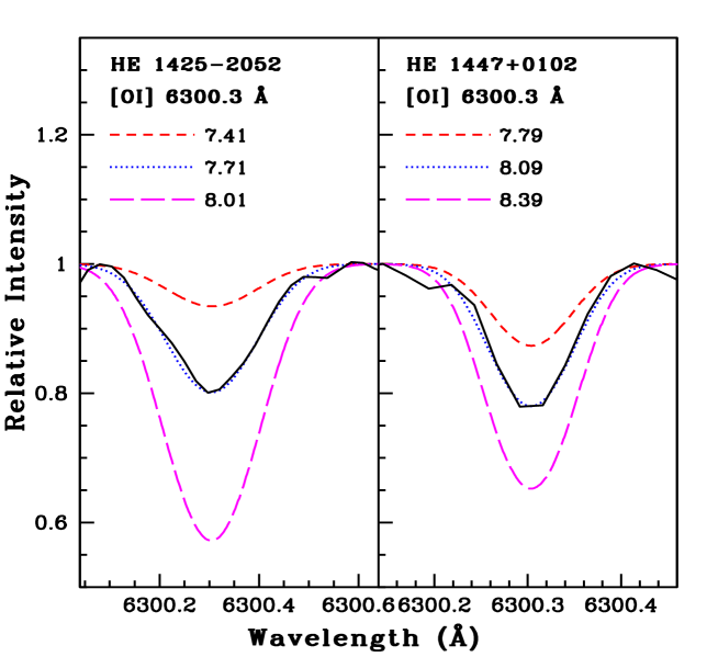
Figure 3: Synthesis of [OI] line around 6300 Å. Dotted line represents synthesized spectra and the solid line indicates the observed spectra. Short dashed line represents the synthetic spectra corresponding to $\Delta$[O/Fe] = -0.2 and long dashed line corresponds to $\Delta$[O/Fe] = +0.2

The abundance of carbon is determined using the spectrum synthesis calculation of the C₂ band at 5165 Å (Figure 4). We could also determine the C abundance using the spectrum synthesis calculation of CH band around 4315 Å only for HE 1428$-$1950 and HE 1425$-$2052. For the remaining stars CH band is found to be saturated except HE 0110$-$0406, and HE 1528$-$0409 for which this region is noisy and not suitable for abundance determination. Since we could determine the abundance of C from the synthesis of C₂ band at 5165 Å for all the stars, we have used this value throughout our analysis. C is enhanced in all the programme stars with [C/Fe] ranging from 0.73 to 2.29. We could estimate the carbon isotopic ratio in all the programme stars. Carbon isotopic ratio is determined from the spectrum synthesis calculation of the C₂ swan system around 4740Å (Figure 5). The estimated values are presented in Table 9.

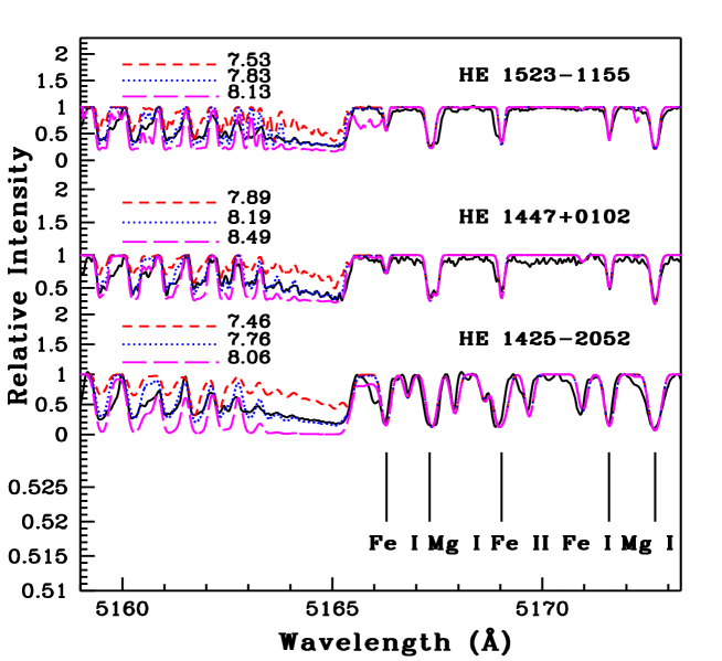
Figure 4: Synthesis of C₂ band around 5165 Å. Dotted line represents synthesized spectra and the solid line indicates the observed spectra. Short dashed line represents the synthetic spectra corresponding to $\Delta$ [C/Fe] = -0.2 and long dashed line corresponds to $\Delta$[C/Fe] = +0.2

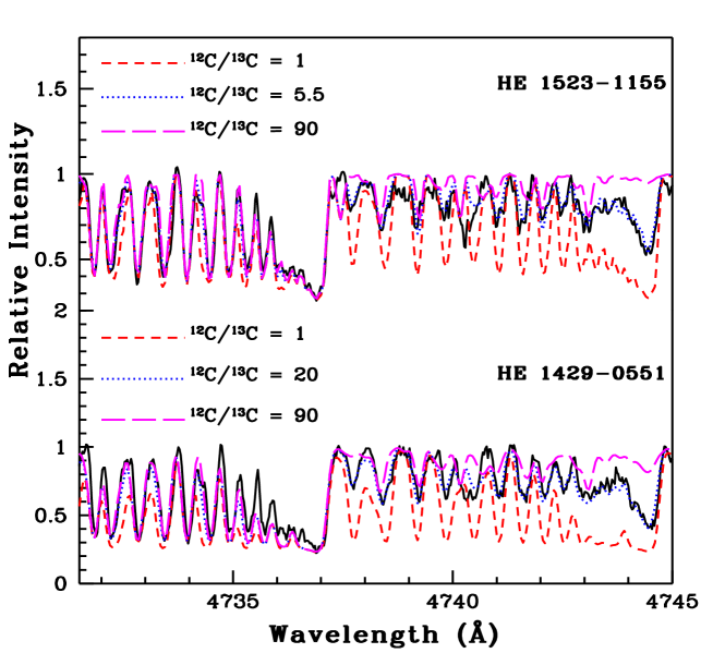
Figure 5: Spectral synthesis fits of the C₂ features around 4740 Å. Solid line indicates the observed spectra. Short and long dashed lines are shown to illustrate the sensitivity of the line strengths to the isotopic carbon abundance ratios

Nitrogen abundance is determined from the spectrum synthesis calculation of CN band at 4215Å (Figure 6). N is enhanced in all the programme stars except HE 1425$-$2052 with [N/Fe] $\sim$ 0.39. The molecular line lists for C and N are adopted from Sneden et al. (2014) and Ram et al. (2014).

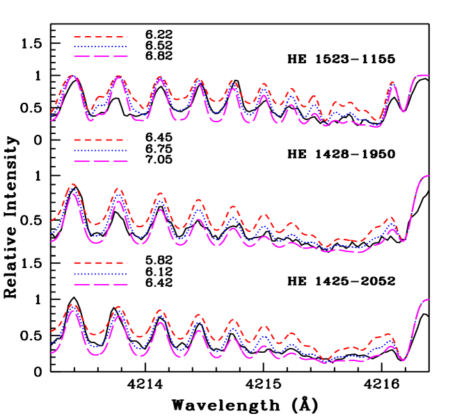
Figure 6: Synthesis of CN band around 4215 Å. Dotted line represents synthesized spectra and the solid line indicates the observed spectra. Short dashed line represents the synthetic spectra corresponding to $\Delta$[N/Fe] = -0.2 and long dashed line corresponds to $\Delta$[N/Fe] = +0.2

6.2 Na, Mg, Ca, Sc, Ti, and V

Abundance of sodium is determined from the equivalent width measurements of three Na I lines (Table 14). HE 1428$-$1950 shows enhancement of Na with [Na/Fe] $\sim$ 1.59. In the remaining objects, Na is moderately enhanced with [Na/Fe] ranging from 0.25 to 0.86, except HE 1528$-$0409 for which [Na/Fe] $\sim$ 0.25. Abundance of magnesium is estimated using the equivalent width measurement of three Mg I lines (Table 14). The estimated values of Mg abundance lie in the range [Mg/Fe] $\sim$ 0.27 to 0.96.

We have used the equivalent width measurements of 11 Calcium I lines (Table 14) to estimate the abundance of Ca in the programme stars. Ca is near solar in HE 1429$-$0551 and HE 0110$-$0406. In the remaining objects, [Ca/Fe] values range from 0.23 to 0.47. The abundance of Scandium is determined using the spectrum synthesis calculation of the lines Sc II 4415.56, 4431.350 and 6245.63 using the hyperfine structures from Prochaska & McWilliam (2000). Sc abundance is found to be near solar in all the programme stars except for HE 1425$-$2052 and HE 1523$-$1155 for which [Sc/Fe] values are 0.44 and 0.35 respectively.

The abundance of titanium is determined using the equivalent width measurements of Ti I and Ti II lines (Table 14). Ti is found to be under abundant in HE 1447+0102 with [Ti/Fe] $\sim$ $-0.28$. In the remaining objects, [Ti/Fe] values are in the range 0.12 to 0.43. The abundance of Vanadium is determined from the spectrum synthesis calculation of the lines V I 4864.73 Å and 5727.05 Å using the hyperfine structures from Prochaska & McWilliam (2000). HE 1428$-$1950 and HE 1528$-$0409 show enhancement of V with [V/Fe] $\sim$ 0.90. While the abundance of V is moderately enhanced in HE 1425$-$2052 and HE 1447+0102, V is marginally enhanced in HE 1429$-$0551 and HE 1523$-$1155. V is found to be under abundant in HE 0110$-$0406.

6.3 Cr, Mn, Co, Ni, and Zn

Abundance of cromium is estimated using the equivalent width measurements of a number of Cr I and Cr II lines (Table 14). While Cr is enhanced in HE 1428$-$1950 with [Cr/Fe] $\sim$ 1.29, it is found to be under abundant in HE 1425$-$2052 with [Cr/Fe] $\sim$ $-0.26$. HE 1523$-$1155 shows moderate enhancement of Cr and near solar values for HE 1429$-$0551 and HE 0110$-$0406. We could not measure Cr in HE 1447+0102 as the lines are found to be blended and not suitable for abundance determination. The abundance of Manganese is determined using the spectrum synthesis calculation of the lines Mn I 4470.14 Å and 6013.51 Å considering the hyperfine structure from Prochaska & McWilliam (2000). [Mn/Fe] values in the programme stars range from $-0.25$ to 0.46.

The abundance of cobalt could be determined only in HE 0110$-$0406, HE 1425$-$2052 and HE 1428$-$1950. The Co I lines are found to be blended in the remaining objects. Co is enhanced in HE 1428$-$1950 with [Co/Fe] $\sim$ 0.93 and near solar in HE 0110$-$0406 and HE 1425$-$2052. The abundance of Nickel could be determined in all the programme stars except for HE 1528$-$0409. In all the stars, Ni is found to be slightly enhanced with [Ni/Fe] in the range 0.26 to 0.45. The abundance of Zinc could be determined only in HE 0110$-$0406, HE 1425$-$2052, HE 1428$-$1950 and HE 1523$-$1155 with [Zn/Fe] in the range $-0.41$ to 0.50. In the remaining stars, the Zn I lines are found to be highly blended and could not be used for abundance calculation.

6.4 Sr, Y, and Zr

The abundance of strontium is determined from the spectrum synthesis calculation of the line Sr I 4607.33 Å. Sr is enhanced in all the programme stars. We could not estimate the abundance of Sr in HE 1429$-$0551 and HE 1528$-$0409 as this region is very noisy and not suitable for abundance calculation.

We have used the equivalent width measurements of three Yttrium II lines (Table 14) for the determination of Y abundance in the programme stars. While Y is enhanced in HE 0110$-$0406, HE 1425$-$2052 and HE 1428$-$1950 with [Y/Fe] $\sim$ 1.28, 1.37, and 1.25 respectively, it is only moderately enhanced in HE 1523$-$1155 with [Y/Fe] $\sim$ 0.68. In the remaining stars, the abundance of Y could not be determined as the lines are blended. We could not determine the abundance of zirconium in any of our programme stars as the lines due to Zr are either blended or the region is found to be noisy and not suitable for abundance determination.

6.5 Ba, La, Ce, Pr, Nd, Sm, and Eu

Abundance of barium is determined from the spectrum synthesis calculations of the lines Ba II 5853.66 and 6141.71 Å using the hyperfine structures of Ba from McWilliam (1998). We could not estimate the Ba abundance in HE 1428$-$1950 as the lines Ba II 5853.66 and 6141.71Å are saturated. We have also checked other lines due to Ba such as 4554.03 and 4934.08 Å in this object; these lines are found to be highly blended and not suitable for abundance calculation. Ba is enhanced in all the remaining programme stars with [Ba/Fe] ranging from 1.61 to 3.21. In HE 1425$-$2052, Ba is found to be highly enhanced with [Ba/Fe] $\sim$ 3.21. We have used the spectrum synthesis calculation of the line Lanthanum II 4921.78 using the hyperfine structure from Jonsell et al. (2006). La is enhanced in all the programme stars with [La/Fe] ranging from $\sim$1.04 to 2.49. The abundance of Cerium is estimated from the equivalent width measurements of ten Ce II lines (Table 14). All the programme stars exhibit enhancement of Ce with [Ce/Fe] ranging from 1.14 to 2.04.

We could determine the abundance of praseodymium only in HE 0110$-$0406, HE 1429$-$0551, HE 1447+0102 and HE 1528$-$0409. In all these stars Pr is found to be enhanced with [Pr/Fe] ranging from 1.09 to 2.05. The abundance of neodymium could be measured in all the programme stars and all of them exhibit enhancement of Nd with [Nd/Fe] in the range 1.03 to 2.34. We could estimate the abundance of samarium in all the programme stars with [Sm/Fe] in the range 1.15 to 2.66. We have used the spectrum synthesis calculation of the lines Europium II 4129.71, 6437.63 and 6645.11 Å to determine the abundance of Eu in the programme stars. The hyperfine structures of Eu are taken from Worley et al. (2013). Eu is enhanced in all the programme stars except HE 0110$-$0406 and HE 1528$-$0409.

We have checked for the lines due to the heavy elements such as Ru I 4869.15 Å, several Nb lines Nb I 4152.50, 5642.09, 5729.18, and 5983.2 Å, Mo I lines at 4904.39, and 5196.04 Å, and Dy I 4923.16 Å. In our programme stars, all these lines are found to either absent or very weak and blended with equivalent widths less than 10mÅ. We have also checked the line Pb I 4057.7Å in the spectrum of HE 0110-0406 and this region is found to be noisy.

We have estimated the values of [ls/Fe], [hs/Fe], [hs/ls] where ls represents light s-process elements (Sr, Y, Zr) and hs represents the heavy s-process elements (Ba, La, Ce, Nd). The estimated values of [hs/ls] and the carbon isotopic ratios are presented in Table 9. Table 10 presents a comparison of the abundances of our programme stars with the literature values.

Table 6: Elemental abundances in HE 0110$-$0406

	Z	solar log$\epsilon^{\ast}$	log$\epsilon$	[X/H]	[X/Fe]
C (C2, 5165 Å)	6	8.43	7.85$\pm$0.20(syn)	$-0.58$	0.73
N (CN, 4215 Å)	7	7.83	7.15$\pm$0.20(syn)	$-0.68$	0.63
Na I	11	6.24	5.53(1)	$-0.71$	0.60
Mg I	12	7.60	6.56(1)	$-1.04$	0.27
Ca I	20	6.34	5.02$\pm$0.13(4)	$-1.32$	$-0.01$
Sc II	21	3.15	1.70$\pm$0.20(1,syn)	$-1.45$	$-0.14$
Ti I	22	4.95	3.76$\pm$0.14(4)	$-1.19$	0.12
V I	23	3.93	2.17$\pm$0.20(1,syn)	$-1.76$	$-0.45$
Cr I	24	5.64	4.29$\pm$0.20(3)	$-1.35$	$-0.04$
Mn I	25	5.43	4.30$\pm$0.20(1,syn)	$-1.13$	0.18
Fe I	26	7.50	6.19$\pm$0.09(27)	$-1.31$	-
Fe II	26	7.50	6.21$\pm$0.12(2)	$-1.29$	-
Co I	27	4.99	3.73$\pm$0.04(3)	$-1.26$	0.05
Ni I	28	6.22	5.36(1)	$-0.86$	0.45
Zn I	30	4.56	2.84(1)	$-1.72$	$-0.41$
Sr I	38	2.87	2.34$\pm$0.20(1,syn)	$-0.53$	0.78
Y II	39	2.21	2.20(1)	$-0.01$	1.28
Ba II	56	2.18	2.50$\pm$0.20(1,syn)	0.32	1.61
La II	57	1.10	1.07$\pm$0.20(1,syn)	$-0.03$	1.26
Ce II	58	1.58	1.49$\pm$0.21(3)	$-0.09$	1.20
Pr II	59	0.72	0.82$\pm$0.09(2)	0.10	1.39
Nd II	60	1.42	1.49$\pm$ 0.18(4)	0.07	1.36
Sm II	62	0.96	0.90$\pm$0.14(4)	$-0.06$	1.23
Eu II	63	0.52	$-0.25$$\pm$0.20(1,syn)	$-0.77$	0.52

^∗ Asplund et al. (2009), The number inside the parenthesis shows the number of lines used for the abundance determination.

Table 7: Elemental abundances in HE 1425$-$2052, HE 1428$-$1950 and HE 1429$-$0551

			HE 1425$-$2052			HE 1428$-$1950			HE 1429$-$0551
	Z	Solar log$\epsilon^{a}$	log$\epsilon$	[X/H]	[X/Fe]	log$\epsilon$	[X/H]	[X/Fe]	log$\epsilon$	[X/H]	[X/Fe]
C (C2, 5165 Å)	6	8.43	7.76$\pm$0.20(syn)	$-0.67$	1.43	7.92$\pm$0.20(syn)	$-0.51$	1.60	8.25$\pm$0.20(syn)	$-0.18$	2.29
C (CH, 4315 Å)	6	8.43	7.72$\pm$0.20(syn)	$-0.71$	1.39	7.95$\pm$0.20(syn)	$-0.48$	1.63	-	-	-
N (CN, 4215 Å)	7	7.83	6.12$\pm$0.20(syn)	$-$1.71	0.39	6.75$\pm$0.20(syn)	$-1.08$	1.03	6.44$\pm$0.20(syn)	$-1.39$	1.08
O	8	8.69	7.71$\pm$0.20(syn)	$-0.98$	1.12	7.84$\pm$0.20(syn)	$-0.85$	1.26	8.10$\pm$0.20(syn)	$-0.59$	1.88
Na I	11	6.24	4.75(1)	$-$1.49	0.61	5.72$\pm$0.20(1,syn)	$-0.52$	1.59	4.63(1)	$-1.61$	0.86
Mg I	12	7.60	5.83(1)	$-$1.77	0.33	5.92$\pm$0.20(1,syn)	$-1.68$	0.43	5.55(1)	$-2.05$	0.42
Ca I	20	6.34	4.59$\pm$0.20 (6)	$-$1.75	0.35	4.70$\pm$0.20(2)	$-1.64$	0.47	3.92$\pm$0.10(3)	$-2.42$	0.05
Sc II	21	3.15	1.50$\pm$0.20(1,syn)	$-$1.65	0.44	1.09$\pm$0.20(1,syn)	$-2.06$	0.09	0.62$\pm$0.20(1,syn)	$-2.53$	$-0.09$
Ti I	22	4.95	3.20$\pm$0.13 (2)	$-$1.75	0.35	-	-	-	2.75(1)	$-2.20$	0.27
Ti II	22	4.95	3.15$\pm$0.20(2)	$-$1.80	0.29	3.14$\pm$0.20(2)	$-1.81$	0.34	2.79$\pm$0.18(3)	$-2.16$	0.28
V I	23	3.93	2.33$\pm$0.20(1,syn)	$-$1.60	0.50	2.73$\pm$0.20(1,syn)	$-1.20$	0.91	1.81$\pm$0.20(1,syn)	$-2.12$	0.35
Cr I	24	5.64	3.28(1)	$-2.36$	$-0.26$	4.81$\pm$0.16(2)	$-0.83$	1.28	3.18(1)	$-2.46$	0.01
Cr II	24	5.64	-	-	-	4.79(1)	$-0.85$	1.30	-	-	-
Mn I	25	5.43	3.08$\pm$0.20(1,syn)	$-$2.35	$-0.25$	3.66$\pm$0.20(1,syn)	$-1.77$	0.34	3.42$\pm$0.20(1,syn)	$-2.01$	0.46
Fe I	26	7.50	5.40$\pm$0.20(28)	$-$2.10	-	5.39$\pm$0.16(27)	$-2.11$	-	5.03$\pm$0.15(31)	$-2.47$	-
Fe II	26	7.50	5.41$\pm$0.16(2)	$-$2.09	-	5.35$\pm$0.16(3)	$-2.15$	-	5.06$\pm$0.13(2)	$-2.44$	-
Co I	27	4.99	2.97(1)	$-$2.02	0.08	3.81(1)	$-1.18$	0.93	-	-	-
Ni I	28	6.22	4.52$\pm$0.16(2)	$-$1.70	0.40	4.38$\pm$0.05(2)	$-1.84$	0.27	4.01(1)	$-2.21$	0.26
Zn I	30	4.56	2.88(1)	$-$1.68	0.42	2.95(1)	$-1.61$	0.50	-	-	-
Sr I	38	2.87	2.31$\pm$0.20(1,syn)	$-$0.56	1.53	1.80$\pm$0.20(1,syn)	$-1.07$	1.04	-	-	-
Y II	39	2.21	1.49$\pm$0.04(2)	$-$0.72	1.37	1.30(1)	$-0.91$	1.25	-	-	-
Ba II	56	2.18	3.30$\pm$0.20(1,syn)	1.12	3.21	-	-	-	1.62$\pm$0.20(1,syn)	$-0.56$	1.88
La II	57	1.10	1.49$\pm$0.20(1,syn)	0.39	2.49	$-0.01$$\pm$0.20(1,syn)	$-1.11$	1.04	$-0.20$$\pm$0.20(1,syn)	$-1.30$	1.14
Ce II	58	1.58	1.70(1)	$-0.14$	1.95	0.57$\pm$0.17(3)	$-1.01$	1.14	1.04$\pm$0.20(4)	$-0.54$	1.90
Pr II	59	0.72	-	-	-	-	-	-	$-0.63$(1)	$-1.35$	1.09
Nd II	60	1.42	1.67$\pm$0.20(6)	0.25	2.34	0.30$\pm$0.06(3)	$-1.12$	1.03	0.72$\pm$0.15(7)	$-0.70$	1.74
Sm II	62	0.96	1.53$\pm$0.20(6)	0.57	2.66	$-0.04$(1)	$1.00$	1.15	0.29(1)	$-0.67$	1.77
Eu II	63	0.52	0.41$\pm$0.20(1,syn)	$-0.11$	1.98	$-0.56$$\pm$0.20(1,syn)	$-1.08$	1.07	$-0.67$$\pm$0.20(1,syn)	$-1.19$	1.25

^a Asplund et al. (2009), The number inside the parenthesis shows the number of lines used for the abundance determination.

Table 8: Elemental abundances in HE 1447+0102, HE 1523$-$1155 and HE 1528$-$0409

			HE 1447+0102			HE 1523$-$1155			HE 1528$-$0409
	Z	Solar log$\epsilon^{a}$	log$\epsilon$	[X/H]	[X/Fe]	log$\epsilon$	[X/H]	[X/Fe]	log$\epsilon$	[X/H]	[X/Fe]
C (C2, 5165 Å)	6	8.43	8.19$\pm$0.20(syn)	$-0.24$	2.05	7.83$\pm$0.20(syn)	$-0.60$	1.83	8.13$\pm$0.20(syn)	$-0.30$	2.07
N (CN, 4215 Å)	7	7.83	7.13$\pm$0.20(syn)	$-0.70$	1.59	6.52$\pm$0.20(syn)	$-1.31$	1.12	7.13$\pm$0.20(syn)	$-0.7$	1.67
O	8	8.69	8.09$\pm$0.20(syn)	$-0.60$	1.69	7.08$\pm$0.20(syn)	$-1.61$	0.82	6.91$\pm$0.20(syn)	$-1.78$	0.59
Na I	11	6.24	4.60$\pm$0.05(2)	$-1.64$	0.65	4.53(1)	$-1.71$	0.72	4.12$\pm$0.08(2)	$-2.12$	0.25
Mg I	12	7.60	5.88$\pm$0.19(2)	$-1.72$	0.57	6.13(1)	$-1.47$	0.96	5.80(1)	$-1.80$	0.57
Ca I	20	6.34	4.28$\pm$0.14(5)	$-2.06$	0.23	4.26$\pm$0.10(5)	$-2.08$	0.35	4.28$\pm$0.12(5)	$-2.06$	0.31
Sc II	21	3.15	1.18$\pm$0.20(1,syn)	$-1.96$	0.24	1.05$\pm$0.20(1,syn)	$-2.10$	0.35	0.90$\pm$0.20(1,syn)	$-2.25$	0.09
Ti I	22	4.95	-	-	-	2.85(1)	$-2.10$	0.33	-	-	-
Ti II	22	4.95	2.46$\pm$0.13(4)	$-2.49$	$-0.28$	2.93$\pm$0.10(4)	$-2.02$	0.43	2.81$\pm$0.13(3)	$-2.14$	0.20
V I	23	3.93	2.27$\pm$0.20(1,syn)	$-1.66$	0.63	1.81$\pm$0.20(1,syn)	$-2.12$	0.31	2.46$\pm$0.20(1,syn)	$-1.47$	0.90
Cr I	24	5.64	-	-	-	3.73$\pm$0.16(2)	$-1.91$	0.52	-	-	-
Cr II	24	5.64	3.72	$-1.92$	0.29	3.64(1)	$-2.00$	0.45	-	-	-
Mn I	25	5.43	3.60$\pm$0.20(1,syn)	$-1.83$	0.46	-	-	-	-	-	-
Fe I	26	7.50	5.21$\pm$0.12(20)	$-2.29$	-	5.07$\pm$0.11(30)	$-2.43$	-	5.13$\pm$0.13(19)	$-2.37$	-
Fe II	26	7.50	5.29$\pm$0.0(2)	$-2.21$	-	5.06(1)	$-2.44$	-	5.16$\pm$0.12(2)	$-2.34$	-
Ni I	28	6.22	4.37(1)	$-1.85$	0.44	4.20$\pm$0.12(3)	$-2.02$	0.41	-	-	-
Zn I	30	4.56	-	-	-	2.54(1)	$-2.02$	0.41	-	-	-
Sr I	38	2.87	2.15$\pm$0.20(1,syn)	$-0.72$	1.57	1.37$\pm$0.20(1,syn)	$-1.50$	0.93	-	-	-
Y II	39	2.21	-	-	-	0.44(1)	$-1.77$	0.68	-	-	-
Ba II	56	2.18	1.90$\pm$0.20(1,syn)	$-0.28$	1.93	1.57$\pm$0.20(1,syn)	$-0.61$	1.83	1.55$\pm$0.20(1,syn)	$-0.63$	1.71
La II	57	1.10	1.01$\pm$0.20(1,syn)	$-0.09$	2.12	0.24$\pm$0.20$\pm$0.20(1,syn)	$-0.86$	1.59	0.09$\pm$0.20(1,syn)	$-1.01$	1.33
Ce II	58	1.58	1.41$\pm$0.12(3)	$-0.17$	2.04	0.70$\pm$0.14(4)	$-0.88$	1.57	1.13$\pm$0.20(2)	$-0.45$	1.89
Pr II	59	0.72	0.46$\pm$0.06(2)	$-0.26$	1.95	-	-	-	0.43$\pm$0.07(2)	$-0.29$	2.05
Nd II	60	1.42	1.26$\pm$0.17(11)	$-0.16$	2.05	0.59$\pm$0.12(8)	$-0.83$	1.62	0.90$\pm$0.20(5)	$-0.52$	1.82
Sm II	62	0.96	1.05$\pm$0.15(3)	0.09	2.30	0.40$\pm$0.18(5)	$-0.56$	1.89	0.99(1)	0.03	2.37
Eu II	63	0.52	0.26$\pm$0.20(1,syn)	$-0.26$	1.95	$-0.59$$\pm$0.20 (1,syn)	$-1.11$	1.34	$-1.36$$\pm$0.20 (1,syn)	$-1.88$	0.46

^a Asplund et al. (2009), The number inside the parenthesis shows the number of lines used for the abundance determination.

Table 9: Estimates of [Fe/H], [ls/Fe], [hs/Fe], [hs/ls] and ¹²C/¹³C

Star name	[Fe/H]	[ls/Fe]	[hs/Fe]	[hs/ls]	12C/13C
HE 0110$-$0406	$-1.30$	1.03	1.36	0.33	45
HE 1425$-$2052	$-$2.10	1.45	2.49	1.04	8.0
HE 1428$-$1950	$-2.13$	1.14	1.07	0.07	23.0
HE 1429$-$0551	$-2.45$	-	1.66	-	20.0
HE 1447+0101	$-2.25$	-	2.03	-	18.0
HE 1523$-$1155	$-2.44$	0.80	1.65	0.85	5.5
HE 1528$-$0409	$-2.35$	-	1.69	-	7.0

Table 10: Comparison of the abundances of our programme stars with the literature values.

Star name	[Fe I/H]	[Fe II/H]	[Fe/H]	[Sr/Fe]	[Y/Fe]	[Ba II/Fe]	Ref
HE 1429$-$0551	$-2.47$	$-2.44$		-	-	1.88	1
	-	-	$-2.70$	-	0.89	1.52	2
	$-2.47$	$-2.48$	$-2.47$	-	-	1.57	3
HE 1447+0102	$-2.29$	$-2.21$	$-2.25$	1.57	-	1.93	1
	$-2.47$	$-2.45$	$-2.46$	-	-	2.70	3
HE 1523$-$1155	$-2.43$	$-2.44$	$-2.43$	0.93	0.68	1.83	1
	$-2.15$	$-2.17$	$-2.16$	-	-	1.72	3
HE 1528$-$0409	$-2.37$	$-2.34$	$-2.35$	-	-	1.71	1
	$-2.61$	$-2.59$	$-2.60$	-	-	2.30	3
Star name	[La II/Fe]	[Ce II/Fe]	[Pr II/Fe]	[NdII/Fe]	[Sm II/Fe]	[Eu II/Fe]	Ref
HE 1429$-$0551	1.14	1.90	1.09	1.74	1.77	1.25	1
	1.30	1.42	1.38	1.43	1.27	1.08	2

1. This work, 2. Karinkuzhi et al. (2021), 3. Aoki et al. (2007)

7 Abundance uncertainties

The total uncertainties in the derived elemental abundances are contributed by random errors and systematic errors. While the uncertainties in the line parameters such as equivalent widths, line blending, and oscillator strength cause random errors, the uncertainties in the stellar atmospheric parameters causes systematic errors. We have followed the procedures as described in Shejeelammal et al. (2021) to calculate the uncertainties on the elemental abundances derived from the equivalent width measurement as well as the spectrum synthesis calculation. The total uncertainties in the estimated elemental abundances, log$\epsilon$ :

$$\sigma^{2}_{log\epsilon}=\sigma^{2}_{ran}+(\frac{\partial log\epsilon}{\partial T})^{2}\sigma_{T_{eff}}^{2}+(\frac{\partial log\epsilon}{\partial logg})^{2}\sigma^{2}_{logg}+(\frac{\partial log\epsilon}{\partial\zeta})^{2}\sigma^{2}_{\zeta}+(\frac{\partial log\epsilon}{\partial[Fe/H]})^{2}\sigma^{2}_{[Fe/H])}~{}~{}~{}~{}~{}~{}~{}~{}~{}~{}(1)$$

where $\sigma^{2}_{ran}$ = $\sigma_{s}/\sqrt{N}$ . $\sigma_{s}$ represents the standard deviation in the elemental abundances derived using N number of lines due to that element. The $\sigma$’s indicate the typical uncertainties in the adopted stellar atmospheric parameters, and are T_eff $\sim$ $\pm$ 100 K, log g $\sim$ $\pm$ 0.2 dex, $\zeta$ $\sim$ $\pm$ 0.2 km s^-1 , and [Fe/H] $\sim$ $\pm$ 0.1 dex. The uncertainty in [X/Fe] is determined using the relation :

$$\sigma^{2}_{[X/Fe]}=\sigma^{2}_{X}+\sigma^{2}_{[Fe/H]}~{}~{}~{}~{}~{}~{}~{}~{}~{}~{}(2)$$

As an example, the differential elemental abundances derived using the equation (2) for the object HE 1523-1155 are given in Table 11. The error for the abundances derived from the spectrum synthesis calculation is taken to be 0.2 dex (indicated by “syn” in Tables 6, 7, 8). This is the minimum change in the abundance value producing well distinguished synthetic spectra with respect to the best fits. For abundances derived using the equivalent width measurements, the errors listed represent the standard deviation (Tables 6, 7, 8).

Table 11: Differential elemental abundances (log$\epsilon$) derived for the object HE 1523$-$1155.

element	$\Delta$ Teff	$\Delta$ log g	$\Delta\zeta$	$\delta$ [Fe/H]	($\sum$ $\sigma^{2}_{i}$)1/2	$\sigma$[X/Fe]
	($\pm$100K)	($\pm$0.2dex)	($\pm$0.2kms-1)	($\pm$0.1 dex)
C	$\pm$0.21	$\mp$0.03	0.00	0.00	0.21	0.31
N	$\pm$0.31	$\mp$0.07	$\pm$0.02	$\pm$0.04	0.32	0.39
O	$\pm$0.05	$\pm$0.06	0.00	$\pm$0.02	0.08	0.24
Na I	$\pm$0.15	$\mp$0.08	$\mp$0.08	$\mp$0.02	0.19	0.22
Mg I	$\pm$0.07	$\mp$0.05	$\mp$0.09	$\mp$0.01	0.12	0.17
Ca I	$\pm$0.08	$\mp$0.02	$\mp$0.05	0.00	0.10	0.15
Sc II	$\pm$0.06	$\pm$0.08	0.00	$\pm$0.02	0.10	0.25
Ti I	$\pm$0.14	$\mp$0.03	$\mp$0.04	$\mp$0.01	0.15	0.19
Ti II	$\pm$0.05	$\pm$0.05	$\mp$0.08	0.00	0.11	0.16
V I	$\pm$0.12	$\mp$0.03	$\mp$0.05	$\mp$0.01	0.13	0.26
Cr I	$\pm$0.13	$\mp$0.02	$\mp$0.08	$\mp$0.01	0.15	0.22
Cr II	$\mp$0.01	$\pm$0.07	$\mp$0.01	$\pm$0.01	0.07	0.13
Fe I	$\pm$0.11	$\pm$0.01	$\pm$0.04	$\mp$0.04	0.12
Fe II	$\pm$0.04	$\pm$0.09	$\mp$0.03	$\pm$0.01	0.10
Ni I	$\pm$0.11	$\mp$0.01	$\mp$0.03	$\mp$0.01	0.11	0.17
Zn I	$\pm$0.04	$\pm$0.03	$\mp$0.02	$\pm$0.01	0.05	0.12
Sr I	$\pm$0.30	$\pm$0.08	$\pm$0.08	$\pm$0.05	0.32	0.40
Y II	$\pm$0.06	$\pm$0.06	$\mp$0.12	$\pm$0.01	0.15	0.18
Ba II	$\pm$0.08	$\mp$0.04	$\mp$0.25	$\mp$0.09	0.28	0.36
La II	$\pm$0.07	$\pm$0.05	$\mp$0.06	0.00	0.10	0.25
Ce II	$\pm$0.07	$\pm$0.06	$\mp$0.06	$\pm$0.01	0.11	0.17
Nd II	$\pm$0.08	$\pm$0.06	$\mp$0.05	$\pm$0.01	0.11	0.16
Sm II	$\pm$0.07	$\pm$0.06	$\mp$0.04	$\pm$0.01	0.10	0.17
Eu II	$\pm$0.04	$\pm$0.06	$\pm$0.02	$\pm$0.02	0.08	0.24

8 Kinematic analysis

Kinematic analysis of the programme stars are performed following a detailed procedure as explained in Purandardas & Goswami (2021). We have used right-handed coordinate system for the determination of space velocities of the programme stars. That is, the three components U, V and W of the space velocities, U is positive in the direction of Galactic center, V is positive in the direction Galactic rotation and W is positive in the direction of the North Galactic Pole (Johnson & Soderblom, 1987). The values of proper motions and parallax required for the calculations of space velocities are taken from SIMBAD and Gaia (Gaia Collaboration et al., 2016, 2018) respectively. We have used our radial velocity estimates for the calculations.

We have determined the probability for a star’s membership into the thin disk, the thick disk or the halo population. Our estimates show that the objects HE 0110$-$0406 and HE 1447+0102 belong to thick disk population with a probability of $\sim$ 94% and 84% respectively. The remaining objects belong to the Halo population with a probability $>$ 81%. The spatial velocities and the probability estimates for the programme stars are presented in Table 12.

Table 12: Spatial velocity and probability estimates for the programme stars

Star name	ULSR	VLSR	WLSR	Vspa	pthin	pthick	phalo	Population
	(kms-1)	(kms-1)	(kms-1)	(kms-1)
HE 0110$-$0406	66.27$\pm$4.91	$-13.36$$\pm$1.88	29.28$\pm$3.96	73.67$\pm$5.64	0.94	0.06	0.00	Thick
HE 1425$-$2052	289.78$\pm$100.54	$-156.13$$\pm$63.38	$-230.36$$\pm$161.09	401.77$\pm$45.33	0.00	0.00	1.00	Halo
HE 1428$-$1950	135.01$\pm$17.25	$-131.24$$\pm$25.52	$-128.65$$\pm$35.87	228.04$\pm$24.33	0.00	0.18	0.81	Halo
HE 1429$-$0551	7.65$\pm$5.19	$-501.65$$\pm$97.37	$-186.93$$\pm$29.35	535.40$\pm$101.39	0.00	0.00	1.00	Halo
HE 1447+0102	$-26.39$$\pm$0.74	$-159.84$$\pm$16.69	$-53.82$$\pm$1.36	170.71$\pm$16.17	0.00	0.84	0.16	Thick
HE 1523$-$1155	$-128.62$$\pm$14.75	$-307.01$$\pm$44.54	66.61$\pm$11.44	339.46$\pm$43.54	0.00	0.00	0.99	Halo
HE 1528$-$0409	117.61$\pm$73.27	$-290.93$$\pm$100.23	$-353.23$$\pm$86.61	472.48$\pm$105.49	0.00	0.00	1.00	Halo

9 Discussion

We have carried out a detailed abundance analysis for a sample of seven objects, one object is found to be metal-poor and the remaining six are found to be very metal-poor stars. Our analysis shows that the objects HE 1447+0102 and HE 1523$-$1155 satisfy the criteria for CEMP-r/s stars ([C/Fe] $>$ 0.7 (Aoki et al., 2007), [Ba/Fe] $\geq$ 1.0, [Eu/Fe] $\geq$ 1.0, 0.0 $\leq$ [Ba/Eu] $\leq$ 1.0 and/or 0.0 $\leq$ [La/Eu] $\leq$ 0.7 (Goswami et al., 2021)) and all the remaining objects satisfy the criteria for CEMP-s stars ([C/Fe] $>$ 0.7 (Aoki et al., 2007), [Ba/Fe] $\geq$ 1.0, [Ba/Eu] $>$ 0.0 (Goswami et al., 2021)). We could not classify HE 1428-1950 based on criteria involving Ba abundance as we could not determine the abundance of Ba in this object.

All the programme stars exhibit enhancement of carbon and nitrogen except HE 1425$-$2052 for which nitrogen is only slightly enhanced. Oxygen is also found to be enhanced in the stars except HE 1523$-$1155 and HE 1528$-0409$. The $\alpha$-elements are found to be slightly enhanced in all the programme stars except HE 0110$-$0406 for which the abundance of $\alpha$-elements are found to be near solar. While HE 1425$-$2052 shows near solar abundance of Fe-peak elements, HE 1428$-$1950 exhibits enhancement of Fe-peak elements except for Ti and Sc. The remaining objects show slight enhancement in Fe-peak elements.

A comparison of the abundances of various elements estimated in our programme stars with their counterparts observed in CEMP-s, CEMP-r/s and CEMP-no stars taken from various sources is shown in the Figures 7 and 8. Although CEMP-s and r/s stars fall at slightly higher metallicity range than CEMP-no stars, all of them exhibit similar $\alpha$ and Fe peak elemental abundance patterns except for Mn and V. A substantial number of CEMP-no stars show [Mn/Fe] and [V/Fe] $<$ 0 unlike CEMP-s and CEMP-r/s stars. Majority of the CEMP-no stars exhibit Na abundance in the range $-$0.50 $<$ [Na/Fe] $<$ 0.50, and CEMP-s and r/s stars show [Na/Fe] $>$ 0. Unlike CEMP-s and CEMP-r/s stars, the heavy elements such as Sr and Ba are found to be underabundant in CEMP-no stars.

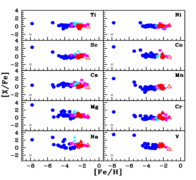
Figure 7: Abundance ratios of light elements with respect to metallicity estimated in our programme stars are represented using red color symbols: HE 0110$-$0406 is represented by open triangle. Filled circle represents HE 1425$-$2052. Filled triangle indicates HE 1428$-$1950. HE 1429$-$0551 is represented by filled square. Filled pentagon represents HE 1447+0102. Filled hexagon and asterisk symbol indicate HE 1523$-$1155 and HE 1528$-$0409 respectively. CEMP-s and CEMP-r/s stars are represented by filled squares (magenta) and filled triangles respectively. Filled circles(blue) represent CEMP-no stars. The abundance values for CEMP-no stars used for the comparison are taken from Christlieb et al. (2004), Plez & Cohen (2005), Yong et al. (2013), Hansen et al. (2014), Bonifacio et al. (2015), Bessell et al. (2015) and Frebel (2018). The abundance values for CEMP-s and CEMP-r/s stars are taken from Lucatello et al. (2003), Barklem et al. (2005), Cohen et al. (2006), Goswami et al. (2006), Aoki et al. (2007), Karinkuzhi & Goswami (2015), Purandardas et al. (2019b), Purandardas et al. (2019a) and Goswami et al. (2021). Representative error bar is shown at the left bottom corner of the figure.

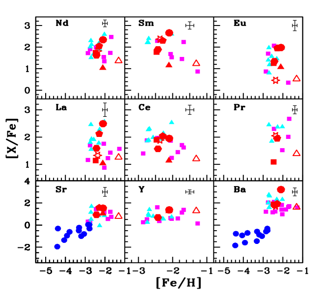
Figure 8: Same as Figure 7, but for heavy elements. Representative error bar is shown at the right top corner of the figure.

The location of a star in the absolute carbon abundance A(C) vs. metallicity [Fe/H] diagram, and various elemental abundance ratios can give important clues about the possible origin of the observed enhancement of carbon as well as neutron-capture elements. A discussion along this line is presented in detail in the following subsections, in the context of the programme stars.

9.1 Locations of the programme stars in the A(C) vs. [Fe/H] diagram:

Many authors have shown that the CEMP stars exhibit bimodal distribution in the A(C) vs. [Fe/H] diagram (Spite et al., 2013; Bonifacio et al., 2015; Hansen et al., 2015; Yoon et al., 2016). While Spite et al. (2013) claimed a higher carbon band around A(C) $\sim$ 8.25 and a lower carbon band around A(C) $\sim$ 6.5, Yoon et al. (2016) suggested a higher carbon band which peaks around A(C) $\sim$ 7.96 and a lower band peaking at A(C) $\sim$ 6.28. Yoon et al. (2016) further classified the objects in the A(C) vs. [Fe/H] diagram into three groups. In this diagram, the objects that show very weak dependence of A(C) on [Fe/H] are called as Group I objects. This group is distributed around the higher carbon band. They are mostly composed of CEMP-s and CEMP-r/s stars and a large fraction of them are confirmed binaries. Group II and Group III objects are extremely metal-poor objects, mostly composed of CEMP-no stars, that are clustered around the lower carbon band. While for Group III objects, A(C) shows no clear dependence on [Fe/H], the A(C) values for Group II objects exhibit very clear dependence on [Fe/H]. A large fraction of Group II and Group III objects are found to be single and hence the observed abundance anomalies are believed to be intrinsic in origin.

The locations of our programme stars in the A(C) vs. [Fe/H] diagram is shown in Figure 9. In order to locate the programme stars in the A(C) vs. [Fe/H] diagram of Yoon et al. (2016), corrections have to be applied to the estimated abundance of carbon. The necessary corrections are applied using the public online tool by Placco et al. (2014) . Table 13 presents the carbon correction and corrected carbon abundances obtained for our programme stars. All of our programme stars are found to be Group I objects in the A(C) vs. [Fe/H] diagram. We therefore expect that the observed enhancement of carbon and heavy elements in these stars may be attributed to a binary companion. But none of the programme stars are confirmed binaries except HE 1523$-$1155.

Table 13: Carbon correction and the corrected carbon abundances obtained for our programme stars

star name	Carbon correction	log$\epsilon$(C)c
HE 0110$-$0406	0.12	7.97
HE 1425$-$2052	0.13	7.89
HE 1428$-$1950	0.12	8.04
HE 1429$-$0551	0.08	8.33
HE 1447+0102	0.06	8.25
HE 1523$-$1155	0.11	7.94
HE 1528$-$0409	0.05	8.18

Note : log$\epsilon$(C)_c represents the carbon abundance after applying the correction.

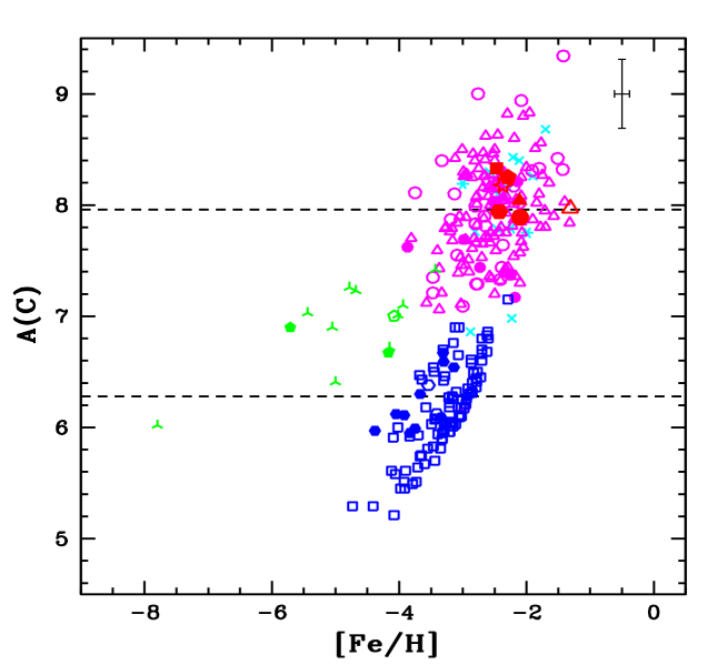
Figure 9: Corrected A(C) vs. [Fe/H] diagram for the compilation of CEMP stars taken from Yoon et al. (2016). Cyan symbols indicate CEMP-r/s stars: binary stars are represented by eight sided star and stars with no information about the binary status are indicated by cross symbols. CEMP-s stars are represented using magenta symbols: Open and filled circles indicates binary and single stars respectively. Stars with no information about the binarity are represented using open triangle. Blue symbols represent Group II CEMP-no stars: Open and filled hexagons represent binary and single stars respectively. Stars with no information about the binarity are presented using open square. Group III CEMP-no stars are represented using green symbols: binary and single stars are represented by open and filled pentagons respectively. Skeleton triangle represents stars with no information about binary status. The symbols used for our programme stars are same as in Figure 7. Representative error bar is shown at the right top corner of the figure.

9.2 Possible progenitors of the programme stars

The enhancement of heavy elements in CEMP-s and CEMP-r/s stars are extrinsic in origin as the evolutionary status of these objects do not support such enhancements. A brief discussion on CEMP-s and CEMP-r/s stars is presented in section 1. As discussed earlier, i-process can well explain the observed over abundances of s- and r-process elements in CEMP-r/s stars. It is found that the neutron densities required for i-process can be achieved in AGB stars during proton ingestion episodes (Cowan & Rose, 1977; Campbell & Lattanzio, 2008; Cristallo et al., 2009a; Campbell et al., 2010; Stancliffe et al., 2011; Banerjee et al., 2018; Clarkson et al., 2018). According to this scenario, a CEMP-r/s star accrets material synthesized by its binary companion during its AGB phase of evolution by i-process nucleosynthesis that can enrich its surface compositions by s- and r- process elements.

Abundance patterns in 20 CEMP-r/s stars could be reproduced by Hampel et al. (2016) based on their i-process model which supports the i-process as the probable mechanism for the formation of CEMP-r/s stars. Hampel et al. (2016) have calculated the yields of heavy elements from i-process nucleosynthesis occurring at different neutron densities based on single-zone nuclear network calculations. We have compared the abundance patterns estimated in the CEMP-r/s stars, HE 1447+0102 and HE 1523$-$1155 with the model yields of Hampel et al. (2016) as shown in Figure 10. The abundance of neutron-capture elements in HE 1447+0102 and HE 1523$-$1155 match well with the expected yields from the i-process nucleosynthesis at a neutron density n $\sim$ 10¹³ with a dilution factor $\sim$ 0.98.

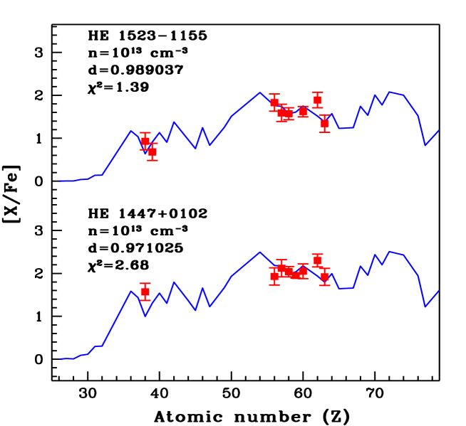
Figure 10: Best-fitting i-process model (solid blue curve) for HE 1447+0102 and HE 1523$-$1155. The points with error bars indicate the observed abundances.

We have compared the abundance patterns of CEMP-s stars in our sample with the model predictions of AGB stars provided by FRANEC Repository of Updated Isotopic Tables & Yields (FRUITY) models (Cristallo et al., 2009b, 2011, 2015); the data are publicly available at http://fruity.oa-teramo.inaf.it/ following the detailed procedure presented in Shejeelammal et al. (2021) . The best fits obtained for the observed abundances are shown in Figures 11 and 12. For the object HE 0110-0406, the best fit is obtained for the model with metallicity, z = 0.001, and mass, M = 1.5M_⊙. For HE 1429-0551, and HE 1528-0409, the model with z = 0.00002 and M = 2M_⊙ gives the best fit. For HE 1425-2052, the best fit is obtained for the model with z = 0.00002, and mass, M = 1.5M_⊙. The observed abundance patterns in HE 1428-1950 could not be matched with any of the available yield values from the FRUITY models.

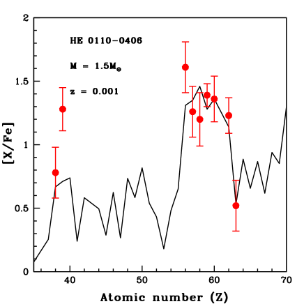
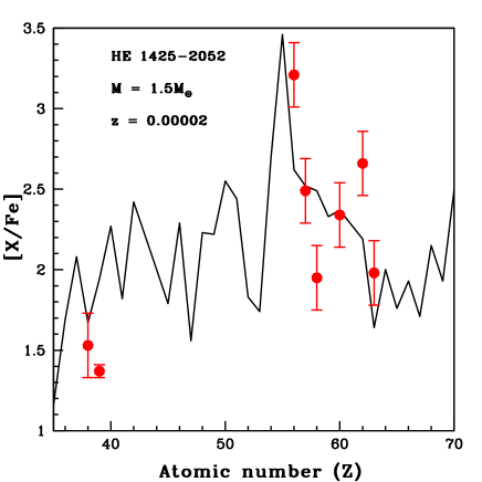
Figure 11: Best-fitting FRUITY model (solid black curve) for HE 0110$-$0406, and HE 1425$-$2052. The points with error bars indicate the observed abundances.

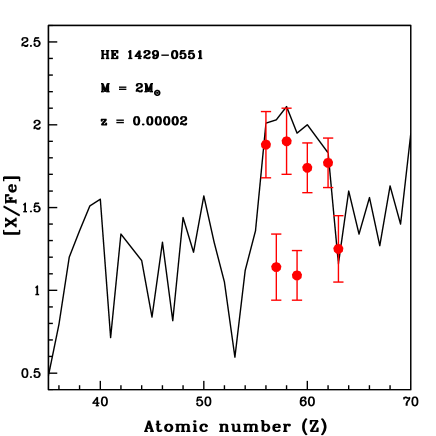
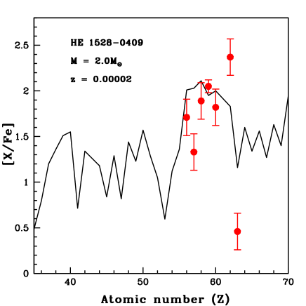
Figure 12: Best-fitting FRUITY model (solid black curve) for HE 1429$-$0551, and HE 1528$-$0409. The points with error bars indicate the observed abundances.

The abundance of oxygen and the [Sr/Ba] ratio can be used as indicators of the possible formation sites of a star (Choplin et al., 2017). Choplin et al. (2017) analysed the abundance patterns of four single CEMP-s stars based on the models of rotating and non-rotating massive stars with masses 10-150 M_⊙. They find that the models of fast rotating massive stars could reproduce the observed abundance patterns in three of the CEMP-s stars in their sample. Their studies show that CEMP-s stars with fast rotating massive star as the progenitor show oxygen abundance in the range between 1.5 to 2. Karakas (2010) predict $-0.2$ $<$ [O/Fe] $<$ 1.2 for CEMP-s stars with AGB progenitors. Studies by Frischknecht et al. (2012) show that [Sr/Ba] $>$ 0 for massive rotating stars. Choplin et al. (2017) also support this idea and they claim that [Sr/Ba] ratio is higher in fast rotating massive stars than in AGB stars.

We could determine [Sr/Ba] ratio in HE 0110$-$0406, HE 1425$-$2052, HE 1447+0102 and HE 1523$-$1155. For all of them the [Sr/Ba] ratio is found to be $<$ 0. This indicates an AGB star as the source of the peculiar abundance patterns in these stars. While the [Sr/Ba] ratio in HE 1447+0102 indicates an AGB star as the progenitor, the [O/Fe] measured in this object is the characteristic of a fast rotating massive star progenitor. This shows that this object may be polluted by multiple events. The [O/Fe] estimated in the remaining stars represent an AGB progenitor except HE 1429$-$0551 and HE 1447+0102. We could measure both [Sr/Ba] ratio and [O/Fe] only in three of the programme stars, HE 1425$-$2052, HE 1447+0102 and HE 1523$-$1155 and their locations in the [Sr/Ba] vs. [O/Fe] diagram are shown in Figure 13.

Estimation of [ls/hs] ratio is another way to find the possible progenitor of a star. While the models of fast rotating massive stars predict [ls/hs] $\geq$ 0 (Choplin et al., 2017; Chiappini, 2013; Cescutti et al., 2013), the AGB models predict [ls/hs] $<$ 0 (Abate et al., 2015). We could measure the [ls/hs] ratio in HE 0110$-$0406, HE 1425$-$2052, HE 1428$-$1950 and HE 1523$-$1155. For all of them, [ls/hs] ratio is found to be $<$ 0. This indicates an AGB progenitor for these objects.

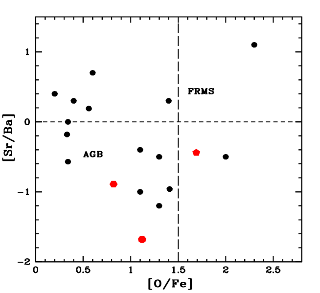
Figure 13: Locations of the programme stars HE 1425$-$2052, HE 1447+0102 and HE 1523$-$1155 in [Sr/Ba] vs. [O/Fe] diagram. Symbols used for the programme stars are same as in Figure 7. Filled circles (black) represent CEMP stars from Hansen et al. (2019)

Elemental abundance ratios such as [Mg/C], [Sc/Mn], [C/Cr] and [Ca/Fe] can also be used to examine whether the star is polluted by a single event or several pollution events. Hartwig et al. (2018) presented a novel diagnostic to identify stars that are formed from the gas enriched by only one previous supernova based on their cosmological models. They showed that [Mg/C] $<$ $-1.0$, [Sc/Mn] $<$ 0.50, [C/Cr] $>$ 0.50 and [Ca/Fe] $>$ 2 represent mono-enrichment of a star. As an example we have shown the locations of our programme stars in the [Mg/C] vs. [Fe/H] diagram (Figure 14). All the programme stars except HE 1523$-$1155 fall in the region representing mono-enrichment. Hansen et al. (2019) show that some of the CEMP-s stars in their sample are also mono-enriched. The estimated value of [Ca/Fe] in all our programme stars show that they are all multi-enriched as expected for CEMP-s and CEMP-r/s stars. The value of [Sc/Mn] measured in all the programme stars except HE 1425$-$2052 show that they are all mono-enriched. The estimated value of [C/Cr] ratio in the programme stars also show that they are mono-enriched except HE 1428$-$1950. Various diagnostic elemental abundance ratios estimated in each of the programme star show that their surface composition is both mono- and multi- enriched which does not fit with the results from Hartwig et al. (2018). This indicates that the different diagnostic elements in our programme stars are not originated from the previous supernova and it may be attributed to their binary companion.

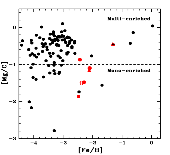
Figure 14: Locations of programme stars in [Mg/C] vs. [Fe/H] plot. Symbols used for the programme stars are same as in Figure 7. Filled circles represent the stars from literature (Roederer et al., 2014; Plez & Cohen, 2005; Christlieb et al., 2004; Hansen et al., 2014; Frebel, 2018; Yong et al., 2013; Bonifacio et al., 2015; Bessell et al., 2015; Lucatello et al., 2003; Barklem et al., 2005; Cohen et al., 2006; Aoki et al., 2007; Goswami et al., 2006; Karinkuzhi & Goswami, 2015; Purandardas et al., 2019b, a; Goswami et al., 2021; Shejeelammal et al., 2021)

9.3 Mixing diagnostic

As all the program stars are luminous objects with log(L/L_⊙) $>$ 2.50, an extra mixing can happen and modify the chemical compositions of the stars (Gratton et al., 2000; Spite et al., 2005). We have therefore examined any possibility of internal mixing processes that could have modified the observed surface compositions of our programme stars using estimates of [C/N] ratios and carbon isotopic ratios. None of the programme stars show any signatures of internal mixing based on [C/N] ratios (Figure 15). Spite et al. (2006) noted that [C/N] ratio is not a clean indicator of mixing as the abundances of carbon and nitrogen in the interstellar medium show large variations. In such cases, carbon isotopic ratio can be used as a good indicator of mixing as it is high in primordial matter and it is insensitive to the choice of atmospheric parameters for the stars (Spite et al., 2006). We could determine ${}^{12}C$/¹³C ratio in all our programme stars and the estimated values of ¹²C/¹³C show that HE 1425$-$2052, HE 1523$-$1155 and HE 1528$-$0409 are well mixed objects (Figure 16).

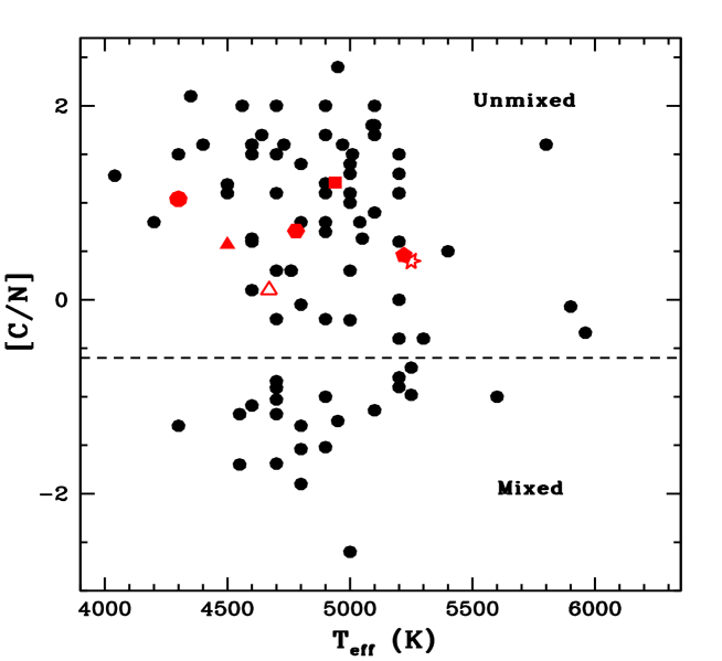
Figure 15: Positions of the programme stars in the [C/N] vs. T_eff diagram. Symbols used for the programme stars are same as in Figure 7. Filled circles represent the stars from literature (Spite et al., 2006; Aoki et al., 2007; Goswami et al., 2016; Hansen et al., 2016b, 2019; Purandardas et al., 2019b, a; Goswami et al., 2021; Shejeelammal et al., 2021)

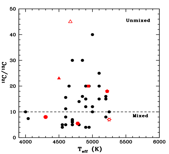
Figure 16: Positions of the programme stars in ¹²C/¹³C vs. T_eff diagram. Symbols used for the programme stars are same as in Figure 7. Open circles represent the stars from Spite et al. (2006) and Aoki et al. (2007)

10 Conclusion

Results from follow-up high resolution spectral analysis of seven potential CH star candidates from Goswami (2005) and Goswami et al. (2010a) are presented. Our analysis shows one object to be metal-poor and the remaining six are very metal-poor stars. For the objects HE 0110$-$0406, HE 1425$-$2052 and HE 1428$-$1950, this work presents for the first time a detailed abundance analysis study. Our analysis shows that the objects HE 1447+0102 and HE 1523$-$1155 to be CEMP-r/s stars. The abundances of neutron-capture elements in HE 1447+0102 and HE 1523$-$1155 show good match with the yields from the i-process nucleosynthesis at a neutron density n $\sim$ 10¹³. Based on our analysis, the objects HE 1425$-$2052, HE 1429$-$0551 and HE 1528$-$0409 are found to be CEMP-s stars. The object HE 1428$-$1950 could not be classified based on CEMP stars classification scheme as we could not estimate the abundance of Ba in this object.

The locations of the programme stars in the absolute carbon abundance, A(C) vs. [Fe/H] diagram show that, they all belong to Group I objects. As most of the Group I objects are known as binaries, the locations of the stars among the Group I objects may indicate binarity. We note that, the object HE 1523$-$1155 in our sample is a confirmed binary (Hansen et al., 2016a).

The estimated [O/Fe] values indicate AGB stars as possible progenitors of the programme stars except for HE 1429$-$0551 and HE 1447+0102. For these two objects, the estimated oxygen abundance characterises fast rotating massive star progenitors.

Other useful indicators of the formation sources of the stars are [Sr/Ba] and [hs/ls] ratios. The estimated [Sr/Ba] ratio in HE 0110$-$0406, HE 1425$-$2052, HE 1447+0102 and HE 1523$-$1155 points at AGB stars as possible progenitors. The estimated [hs/ls] ratio in HE 0110$-$0406, HE 1425$-$2052, HE 1428$-$1950 and HE 1523$-$1155 also indicate AGB stars as possible progenitors.

We have also studied the chemical enrichment histories of the programme stars based on various other elemental abundance ratios such as [Mg/C], [Sc/Mn] and [C/Cr]. While HE 1425$-$2052 is found to be multi-enriched, remaining stars are all found to be mono-enriched based on [Sc/Mn] ratio. The estimated [C/Cr] ratio in the programme stars also shows that they are mono-enriched except for HE 1428$-$1950. All the stars are also found to be mono-enriched based on [Mg/C] ratio, except for HE 1523$-$1155. The estimated Ca abundance of the stars show that their surface composition is enriched by multiple pollution events.

The programme stars are luminous with log(L/L_⊙) $>$ 2. In order to understand whether any internal mixing processes have modified their surface compositions, we have looked for signatures of internal mixing in our programme stars based on the estimates of the [C/N] and ¹²C/¹³C ratios. While the [C/N] ratio estimated in the programme stars show that they are all unmixed, the estimated carbon isotopic ratios show that HE 1425$-$2052, HE 1523$-$1155 and HE 1528$-$0409 are well mixed.

Kinematic analysis shows that the objects HE 0110$-$0406 and HE 1447+0102 to be thick disk objects and the remaining objects belong to the halo population of the Galaxy.

The estimates of abundance ratios presented in this paper can be used for theoretical studies to constrain the physics and the nucleosynthesis occurring in low-mass AGB stars. Abundance results of CEMP-r/s stars will also provide observational constrains for i-process nucleosynthesis which is believed to be the possible source of the origin of the peculiar chemical abundance patterns observed in CEMP-r/s stars.

11 ACKNOWLEDGEMENT

Funding from the DST SERB project EMR/2016/005283 is gratefully acknowledged. We are thankful to Melanie Hampel for providing us with the i-process yields in the form of number fractions, and Partha Pratim Goswami for helping us to generate the model fits. We thank the referee for many constructive suggestions and useful comments on the manuscript which improved this paper.This work made use of the SIMBAD astronomical database, operated at CDS, Strasbourg, France, the NASA ADS, USA and data from the European Space Agency (ESA) mission Gaia (https://www.cosmos.esa.int/gaia), processed by the Gaia Data Processing and Analysis Consortium (DPAC, https://www.cosmos.esa.int/web/gaia/dpac/consortium).

12 Data Availability

The data underlying this article will be shared on reasonable request to the authors.

Appendix A Lines used for deriving elemental abundances

Table 14: Lines used for deriving elemental abundances in our programme stars

Wavelength(Å)	Element	$E_{low}$(eV)	log gf	HE 0110-0406	HE 1425-2052	HE 1428-1950	HE 1429-0551	HE 1447+0102	HE 1523-1155	HE 1528-0409
5682.633	Na I	2.102	-0.700	79.3(5.53)	50.1(4.75)	-	-	-	-	-
5889.951		0.000	0.100	-	-	-	192.2(4.63)	162.5(4.56)	-	130.6(4.06)
5895.920		0.000	-0.200	-	-	-	-	148.0(4.64)	180.2(4.53)	121.5(4.17)
5172.684	Mg I	2.711	-0.402	-	-	-	172.2(5.55)	167.6(5.75)	-	-
5528.405		4.346	-0.620	-	-	-	-	81.7(6.02)	101.5(6.13)	70.0(5.80)
5711.088		4.346	-1.833	73.3(6.56)	47.0(5.83)	-	-	-	-	-
4318.652	Ca I	1.899	-0.208	-	-	-	41.0(3.82)	-	59.4(4.11)	-
5512.980		2.932	-0.290	47.4(4.85)	-	-	-	-	-	-
5581.965		2.523	-0.710	-	58.5(4.50)	-	-	-	-	-
5588.749		2.525	0.210	-	-	122.4(4.84)	35.8(3.91)	42.0(4.21)	59.6(4.28)	50.3(4.41)
5590.114		2.521	-0.710	68.7(5.12)	-	-	-	-	-	-
5857.451		2.932	0.230	-	107.1(4.68)	-	-	22.7(4.18)	35.5(4.23)	20.5(4.13)
6102.723		1.879	-0.890	100.1(4.98)	119.9(4.52)	88.2(4.55)	25.0(4.01)	35.7(4.47)	46.0(4.32)	30.6(4.38)
6162.173		1.899	0.100	-	-	-	-	66.4(4.15)	95.2(4.38)	70.7(4.29)
6169.563		2.525	-0.270	-	77.6(4.25)	-	-	-	-	-
6439.075		2.525	0.470	142.9(5.14)	172.1(4.65)	-	-	64.4(4.40)	-	53.1(4.18)
6471.662		2.525	-0.590	-	111.5(4.95)	-	-	-	-	-
4415.557	Sc II	0.595	-0.640	-	142.1(1.38)	-	79.5(1.03)	78.3(1.38)	88.6(1.24)	-
4431.352		0.605	-1.880	-	74.8(1.58)	52.6(1.09)	-	-	20.6(0.87)	-
5239.813		1.455	-0.770	-	-	-	30.6(1.01)	45.6(1.59)	42.9(1.23)	36.7(1.45)
5526.790		1.768	0.130	123.7(2.00)	-	-	-	-	-	-
6245.637		1.507	-0.980	85.3(1.99)	65.8(1.55)	-	-	-	26.4(1.09)	-
4555.484	Ti I	0.848	-0.488	83.9(3.75)	-	-	-	-	-	-
4759.270		2.255	0.514	-	-	-	-	-	-	-
4820.410		1.500	-0.441	-	-	-	-	-	-	-
4840.874		0.899	-0.509	72.8(3.58)	113.0(3.30)	-	-	-	-	-
5024.844		0.818	-0.602	88.2(3.80)	-	-	-	-	-	-
5210.385		0.047	-0.884	-	-	-	35.4(2.75)	-	52.1(2.85)	-
5282.376		1.052	-1.300	37.0(3.92)	-	-	-	-	-	-
5922.109		1.046	-1.466	-	23.1(3.11)	-	-	-	-	-
4443.794	Ti II	1.080	-0.700	-	-	-	-	86.6(2.63)	-	-
4468.507		1.130	-0.600	-	-	-	113.3(2.94)	-	115.2(2.94)	-
4470.857		1.164	-2.280	-	-	78.2(2.95)	-	-	-	-
4563.761		1.221	-0.960	-	-	-	-	62.1(2.33)	-	71.4(2.66)
4583.409		1.164	-2.720	-	62.9(3.36)	-	-	-	-	-
4764.526		1.236	-2.770	-	-	-	-	-	22.0(2.95)	-
5185.913		1.892	-1.350	-	68.4(2.94)	-	50.5(2.88)	20.2(2.40)	46.8(2.80)	-
5188.680		1.580	-1.210	-	-	-	-	-	-	59.7(2.91)
5226.543		1.565	-1.300	-	-	154.5(3.39)	68.0(2.80)	38.3(2.47)	78.8(3.03)	54.5(2.86)
5418.751		1.581	-1.999	-	-	-	-	-	-	-
4379.230	V I	0.300	0.580	-	-	-	-	48.2(2.19)	-	-
4864.731		0.017	-0.960	-	-	127.7(3.36)	-	-	-	-
5703.575		1.050	-0.211	-	-	87.5(3.29)	-	-	-	-
5737.059		1.063	-0.740	47.8(3.50)	25.3(2.46)	-	-	-	-	-
6119.523		1.063	-0.320	-	70.3(2.63)	-	-	-	-	-
6216.354		0.275	-1.290	66.1(3.27)	39.2(2.11)	-	-	-	-	-
6251.827		0.286	-1.340	-	-	88.7(3.34)	-	-	-	-
4652.157	Cr I	1.003	-1.030	-	-	178.8(4.92)	-	-	-	-
4829.371		2.544	-0.810	-	-	52.2(4.70)	-	-	-	-
4870.797		3.079	0.050	44.2(4.40)	-	-	-	-	-	-
5296.691		0.982	-1.400	-	-	-	-	-	59.7(3.84)	-
5345.796		1.003	-0.980	134.7(4.41)	-	-	-	-	67.7(3.62)	-
5348.315		1.003	-1.290	98.5(4.06)	108.5(3.28)	-	23.8(3.18)	-	-	-
4848.235	Cr II	3.864	-1.140	-	-	112.8(4.79)	-	20.6(3.72)	27.4(3.64)	-
4451.586	Mn I	2.888	0.278	-	-	105.3(4.26)	-	-	-	-
4470.144		2.941	-0.444	-	30.0(3.31)	-	-	-	-	-
4739.087		2.941	-0.490	64.3(4.40)	-	-	-	-	-	-
4765.846		2.941	-0.080	-	39.8(3.07)	60.2(3.82)	-	-	-	-
4783.427		2.298	0.042	-	-	121.7(3.82)	-	-	-	-
4823.524		2.319	0.144	-	-	131.9(3.90)	-	-	-	-
4792.846	Co I	3.252	-0.067	25.9(3.68)	-	-	-	-	26.9(3.86)	-
4813.467		3.216	0.050	38.6(3.77)	19.7(2.97)	45.5(3.81)	-	-	-	-
5483.344		1.710	-1.490	59.9(3.73)	-	-	-	-	-	-
4980.166	Ni I	3.606	0.070	-	-	-	-	-	42.5(4.31)	-
6314.653		1.935	-1.770	-	-	106.9(4.41)	-	-	-	-
6643.629		1.676	-2.300	129.9(5.36)	125.5(4.41)	88.2(4.35)	21.3(4.01)	22.9(4.37)	33.2(4.08)	-
6767.768		1.826	-2.170	-	138.7(4.63)	-	-	-	36.9(4.20)	-
4810.528	Zn I	4.077	-0.137	56.0(2.84)	61.4(2.88)	78.2(2.95)	-	-	35.6(2.54)	-
4607.327	Sr I	0.000	-0.570	63.0(2.49)	114.1(2.46)	37.9(1.97)	-	27.9(2.51)	-	-

Wavelength(Å)	Element	$E_{low}$(eV)	log gf	HE 0110-0406	HE 1425-2052	HE 1428-1950	HE 1429-0551	HE 1447+0102	HE 1523-1155	HE 1528-0409
4883.684	Y II	1.084	0.070	-	171.7(1.51)	142.3(1.30)	-	-	67.8(0.44)	-
5087.416		1.084	-0.170	-	-	-	-	-	-	-
6613.733		1.748	-1.110	80.7(2.20)	40.9(1.46)	-	-	-	-	-
4130.645	Ba II	2.722	0.680	-	-	-	-	-	71.7(1.63)	-
5853.668		0.604	-1.000	145.1(1.41)	-	-	125.0(1.74)	131.7(2.36)	-	106.3(1.99)
6141.713		0.703	-0.076	-	-	-	163.9(1.49)	-	168.2(1.35)	180.6(2.16)
6496.897		0.604	-0.377	-	-	-	-	-	-	154.7(2.04)
4322.503	La II	0.173	-1.120	-	-	-	40.0(0.33)	47.9(0.90)	36.4(0.17)	39.8(0.75)
4662.498		0.000	-1.240	-	149.7(1.34)	-	-	-	-	-
4748.726		0.926	-0.860	-	101.8(1.43)	-	-	39.7(1.20)	-	-
4921.776		0.244	-0.680	-	-	-	69.4(0.60)	68.9(1.07)	64.9(0.40)	53.0(0.67)
5259.379		0.173	-1.760	-	143.4(1.79)	-	-	-	-	-
5303.528		0.321	-1.430	-	124.9(1.39)	-	-	-	20.0(0.13)	-
6320.376		0.172	-1.610	-	-	-	-	38.0(0.94)	-	-
6390.477		0.321	-1.450	-	-	-	-	-	-	20.4(0.56)
4336.244	Ce II	0.703	-0.564	-	-	-	25.6(0.81)	-	-	-
4418.780		0.863	0.177	-	-	68.2(0.44)	-	-	-	-
4427.916		0.535	-0.460	-	-	59.7(0.52)	-	-	-	28.2(0.96)
4523.075		0.516	-0.304	-	-	-	-	-	47.6(0.74)	-
4539.745		0.327	-0.459	-	-	-	-	-	54.5(0.84)	50.6(1.31)
4544.953		0.417	-0.974	-	-	-	-	31.3(1.34)	-	-
4562.359		0.477	0.081	-	-	-	82.9(1.37)	-	55.8(0.51)	-
4725.069		0.521	-1.204	62.5(1.70)	86.1(1.70)	-	20.1(1.04)	20.7(1.33)	-	-
5330.556		0.869	-0.760	43.5(1.27)	-	40.2(0.76)	20.4(0.95)	30.7(1.54)	20.2(0.72)	-
5556.941		1.813	-0.405	18.1(1.50)	-	-	-	-	-	-
5219.045	Pr II	0.795	-0.240	-	-	-	23.6(-0.63)	-	-	-
5259.728		0.633	0.080	-	-	-	-	-	-	-
5292.619		0.648	-0.300	71.8(0.88)	-	-	-	22.4(0.50)	-	20.5(0.38)
5322.772		0.482	-0.315	75.4(0.76)	-	-	-	25.4(0.41)	-	26.0(0.48)
5892.251		1.439	-0.352	-	-	-	-	-	-	-
6278.676		1.196	-0.630	-	-	-	-	-	-	-
4412.256	Nd II	0.063	-1.420	-	-	-	-	31.9(1.22)	-	-
4446.384		0.204	-0.590	-	-	-	48.3(0.54)	52.7(1.09)	50.8(0.52)	-
4451.563		0.380	-0.040	-	-	105.0(0.37)	75.4(0.97)	68.2(1.24)	-	-
4516.346		0.320	-0.950	-	-	-	40.3(0.84)	46.5(1.39)	-	26.2(0.94)
4797.153		0.559	-0.950	-	99.5(1.45)	-	-	-	25.0(0.66)	-
4825.478		0.182	-0.860	-	-	69.3(0.25)	-	46.7(1.10)	-	-
4859.026		0.320	-0.830	-	143.1(1.65)	61.7(0.29)	-	35.0(0.94)	50.6(0.82)	-
5212.361		0.204	-0.870	93.0(1.24)	169.2(1.79)	-	46.6(0.67)	57.9(1.39)	42.2(0.48)	34.5(0.87)
5255.506		0.204	-0.820	-	146.2(1.39)	-	53.3(0.76)	-	52.4(0.65)	26.7(0.62)
5287.133		0.744	-1.300	-	91.0(1.84)	-	-	-	-	-
5293.163		0.822	-0.060	-	-	-	47.7(0.60)	64.8(1.48)	47.1(0.52)	39.8(0.87)
5319.815		0.550	-0.210	-	-	-	56.3(0.62)	69.5(1.45)	60.4(0.64)	57.7(1.19)
5356.967		1.264	-0.250	76.9(1.62)	-	-	-	27.9(1.20)	-	-
5442.264		0.680	-0.910	81.0(1.61)	-	-	-	-	-	-
5702.238		0.744	-0.770	81.4(1.51)	138.7(1.88)	-	-	37.1(1.33)	19.0(0.44)	-
4220.661	Sm II	0.544	-1.114	-	-	-	-	24.0(0.99)	-	-
4424.337		0.485	-0.260	-	-	-	-	-	45.5(0.16)	55.7(0.99)
4434.318		0.378	-0.576	-	158.1(1.70)	59.5(-0.04)	40.3(0.29)	-	51.1(0.48)	-
4499.475		0.248	-1.413	-	92.7(1.24)	-	-	-	20.0(0.33)	-
4519.630		0.543	-0.751	-	-	-	-	38.0(0.94)	32.2(0.39)	-
4566.202		0.333	-1.245	-	100.3(1.28)	-	-	38.7(1.22)	33.4(0.65)	-
4615.444		0.543	-1.262	-	98.8(1.55)	-	-	-	-	-
4674.593		0.184	-1.055	65.7(0.72)	-	-	-	-	-	-
4726.026		0.333	-1.849	25.0(0.92)	-	-	-	-	-	-
4791.580		0.104	-1.846	47.8(1.07)	119.5(1.79)	-	-	-	-	-
4854.368		0.378	-1.873	20.3(0.87)	79.7(1.61)	-	-	-	-	-
4129.730	Eu II	0.000	0.204	-	-	-	-	74.9(0.11)	-	22.3(-1.45)
6437.640		1.319	-0.276	-	70.1(0.49)	-	-	22.4(0.25)	-	-
6645.064		1.379	0.204	-	89.3(0.31)	64.6(-0.35)	-	-	-	-

The numbers in the parenthesis in columns 5-11 give the derived abundances from the respective line. log gf values are taken from kurucz atomic line list (https://www.cfa.harvard.edu).

References

- Abate et al. (2015) Abate, C., Pols, O. R., Izzard, R. G., & Karakas, A. I. 2015, A&A, 581, A22, doi: 10.1051/0004-6361/201525876
- Abate et al. (2016) Abate, C., Stancliffe, R. J., & Liu, Z.-W. 2016, A&A, 587, A50, doi: 10.1051/0004-6361/201527864
- Alonso et al. (1999) Alonso, A., Arribas, S., & Martínez-Roger, C. 1999, A&AS, 140, 261, doi: 10.1051/aas:1999521
- Aoki et al. (2007) Aoki, W., Beers, T. C., Christlieb, N., et al. 2007, ApJ, 655, 492, doi: 10.1086/509817
- Arentsen et al. (2019) Arentsen, A., Starkenburg, E., Shetrone, M. D., et al. 2019, A&A, 621, A108, doi: 10.1051/0004-6361/201834146
- Asplund et al. (2009) Asplund, M., Grevesse, N., Sauval, A. J., & Scott, P. 2009, ARA&A, 47, 481, doi: 10.1146/annurev.astro.46.060407.145222
- Banerjee et al. (2018) Banerjee, P., Qian, Y.-Z., & Heger, A. 2018, MNRAS, 480, 4963, doi: 10.1093/mnras/sty2251
- Barbuy et al. (1997) Barbuy, B., Cayrel, R., Spite, M., et al. 1997, A&A, 317, L63
- Barbuy et al. (2005) Barbuy, B., Spite, M., Spite, F., et al. 2005, A&A, 429, 1031, doi: 10.1051/0004-6361:20040415
- Barklem et al. (2005) Barklem, P. S., Christlieb, N., Beers, T. C., et al. 2005, A&A, 439, 129, doi: 10.1051/0004-6361:20052967
- Beers & Christlieb (2005) Beers, T. C., & Christlieb, N. 2005, ARA&A, 43, 531, doi: 10.1146/annurev.astro.42.053102.134057
- Beers et al. (2007) Beers, T. C., Flynn, C., Rossi, S., et al. 2007, ApJS, 168, 128, doi: 10.1086/509324
- Bessell et al. (2015) Bessell, M. S., Collet, R., Keller, S. C., et al. 2015, ApJ, 806, L16, doi: 10.1088/2041-8205/806/1/L16
- Bisterzo et al. (2011) Bisterzo, S., Gallino, R., Straniero, O., Cristallo, S., & Käppeler, F. 2011, MNRAS, 418, 284, doi: 10.1111/j.1365-2966.2011.19484.x
- Bonifacio et al. (2015) Bonifacio, P., Caffau, E., Spite, M., et al. 2015, A&A, 579, A28, doi: 10.1051/0004-6361/201425266
- Campbell & Lattanzio (2008) Campbell, S. W., & Lattanzio, J. C. 2008, A&A, 490, 769, doi: 10.1051/0004-6361:200809597
- Campbell et al. (2010) Campbell, S. W., Lugaro, M., & Karakas, A. I. 2010, A&A, 522, L6, doi: 10.1051/0004-6361/201015428
- Cescutti et al. (2013) Cescutti, G., Chiappini, C., Hirschi, R., Meynet, G., & Frischknecht, U. 2013, A&A, 553, A51, doi: 10.1051/0004-6361/201220809
- Chiappini (2013) Chiappini, C. 2013, Astronomische Nachrichten, 334, 595, doi: 10.1002/asna.201311902
- Choplin et al. (2017) Choplin, A., Hirschi, R., Meynet, G., & Ekström, S. 2017, A&A, 607, L3, doi: 10.1051/0004-6361/201731948
- Christlieb et al. (2004) Christlieb, N., Beers, T. C., Barklem, P. S., et al. 2004, A&A, 428, 1027, doi: 10.1051/0004-6361:20041536
- Clarkson et al. (2018) Clarkson, O., Herwig, F., & Pignatari, M. 2018, MNRAS, 474, L37, doi: 10.1093/mnrasl/slx190
- Cohen et al. (2003) Cohen, J. G., Christlieb, N., Qian, Y. Z., & Wasserburg, G. J. 2003, ApJ, 588, 1082, doi: 10.1086/374269
- Cohen et al. (2006) Cohen, J. G., McWilliam, A., Shectman, S., et al. 2006, AJ, 132, 137, doi: 10.1086/504597
- Cowan & Rose (1977) Cowan, J. J., & Rose, W. K. 1977, ApJ, 212, 149, doi: 10.1086/155030
- Cristallo et al. (2009a) Cristallo, S., Piersanti, L., Straniero, O., et al. 2009a, PASA, 26, 139, doi: 10.1071/AS09003
- Cristallo et al. (2009b) Cristallo, S., Straniero, O., Gallino, R., et al. 2009b, ApJ, 696, 797, doi: 10.1088/0004-637X/696/1/797
- Cristallo et al. (2015) Cristallo, S., Straniero, O., Piersanti, L., & Gobrecht, D. 2015, ApJS, 219, 40, doi: 10.1088/0067-0049/219/2/40
- Cristallo et al. (2011) Cristallo, S., Piersanti, L., Straniero, O., et al. 2011, ApJS, 197, 17, doi: 10.1088/0067-0049/197/2/17
- Cutri et al. (2003) Cutri, R. M., Skrutskie, M. F., van Dyk, S., et al. 2003, VizieR Online Data Catalog, II/246
- Dardelet et al. (2015) Dardelet, L., Ritter, C., Prado, P., et al. 2015, in Proceedings of XIII Nuclei in the Cosmos — PoS(NIC XIII), Vol. 204, 145, doi: 10.22323/1.204.0145
- Denissenkov et al. (2017) Denissenkov, P. A., Herwig, F., Battino, U., et al. 2017, ApJ, 834, L10, doi: 10.3847/2041-8213/834/2/L10
- Denissenkov et al. (2019) Denissenkov, P. A., Herwig, F., Woodward, P., et al. 2019, MNRAS, 488, 4258, doi: 10.1093/mnras/stz1921
- Frebel (2018) Frebel, A. 2018, Annual Review of Nuclear and Particle Science, 68, 237, doi: 10.1146/annurev-nucl-101917-021141
- Frischknecht et al. (2012) Frischknecht, U., Hirschi, R., & Thielemann, F. K. 2012, A&A, 538, L2, doi: 10.1051/0004-6361/201117794
- Gaia Collaboration et al. (2016) Gaia Collaboration, Prusti, T., de Bruijne, J. H. J., et al. 2016, A&A, 595, A1, doi: 10.1051/0004-6361/201629272
- Gaia Collaboration et al. (2018) Gaia Collaboration, Brown, A. G. A., Vallenari, A., et al. 2018, A&A, 616, A1, doi: 10.1051/0004-6361/201833051
- Goswami (2005) Goswami, A. 2005, MNRAS, 359, 531, doi: 10.1111/j.1365-2966.2005.08917.x
- Goswami et al. (2006) Goswami, A., Aoki, W., Beers, T. C., et al. 2006, MNRAS, 372, 343, doi: 10.1111/j.1365-2966.2006.10877.x
- Goswami et al. (2016) Goswami, A., Aoki, W., & Karinkuzhi, D. 2016, MNRAS, 455, 402, doi: 10.1093/mnras/stv2011
- Goswami & Karinkuzhi (2013) Goswami, A., & Karinkuzhi, D. 2013, A&A, 549, A68, doi: 10.1051/0004-6361/201219911
- Goswami et al. (2010a) Goswami, A., Karinkuzhi, D., & Shantikumar, N. S. 2010a, MNRAS, 402, 1111, doi: 10.1111/j.1365-2966.2009.15939.x
- Goswami et al. (2010b) Goswami, A., Kartha, S. S., & Sen, A. K. 2010b, ApJ, 722, L90, doi: 10.1088/2041-8205/722/1/L90
- Goswami et al. (2021) Goswami, P. P., Rathour, R. S., & Goswami, A. 2021, A&A, 649, A49, doi: 10.1051/0004-6361/202038258
- Gratton et al. (2000) Gratton, R. G., Sneden, C., Carretta, E., & Bragaglia, A. 2000, A&A, 354, 169
- Hampel et al. (2019) Hampel, M., Karakas, A. I., Stancliffe, R. J., Meyer, B. S., & Lugaro, M. 2019, ApJ, 887, 11, doi: 10.3847/1538-4357/ab4fe8
- Hampel et al. (2016) Hampel, M., Stancliffe, R. J., Lugaro, M., & Meyer, B. S. 2016, ApJ, 831, 171, doi: 10.3847/0004-637X/831/2/171
- Hansen et al. (2019) Hansen, C. J., Hansen, T. T., Koch, A., et al. 2019, A&A, 623, A128, doi: 10.1051/0004-6361/201834601
- Hansen et al. (2011) Hansen, T., Andersen, J., Nordström, B., Buchhave, L. A., & Beers, T. C. 2011, ApJ, 743, L1, doi: 10.1088/2041-8205/743/1/L1
- Hansen et al. (2014) Hansen, T., Hansen, C. J., Christlieb, N., et al. 2014, ApJ, 787, 162, doi: 10.1088/0004-637X/787/2/162
- Hansen et al. (2015) —. 2015, ApJ, 807, 173, doi: 10.1088/0004-637X/807/2/173
- Hansen et al. (2016a) Hansen, T. T., Andersen, J., Nordström, B., et al. 2016a, A&A, 588, A3, doi: 10.1051/0004-6361/201527409
- Hansen et al. (2016b) —. 2016b, A&A, 586, A160, doi: 10.1051/0004-6361/201527235
- Hartwig et al. (2018) Hartwig, T., Yoshida, N., Magg, M., et al. 2018, MNRAS, 478, 1795, doi: 10.1093/mnras/sty1176
- Heger & Woosley (2010) Heger, A., & Woosley, S. E. 2010, ApJ, 724, 341, doi: 10.1088/0004-637X/724/1/341
- Hill et al. (2000) Hill, V., Barbuy, B., Spite, M., et al. 2000, A&A, 353, 557
- Johnson & Soderblom (1987) Johnson, D. R. H., & Soderblom, D. R. 1987, AJ, 93, 864, doi: 10.1086/114370
- Jonsell et al. (2006) Jonsell, K., Barklem, P. S., Gustafsson, B., et al. 2006, A&A, 451, 651, doi: 10.1051/0004-6361:20054470
- Jorissen et al. (2016) Jorissen, A., Hansen, T., Van Eck, S., et al. 2016, A&A, 586, A159, doi: 10.1051/0004-6361/201526993
- Karakas (2010) Karakas, A. I. 2010, MNRAS, 403, 1413, doi: 10.1111/j.1365-2966.2009.16198.x
- Karinkuzhi & Goswami (2015) Karinkuzhi, D., & Goswami, A. 2015, MNRAS, 446, 2348, doi: 10.1093/mnras/stu2079
- Karinkuzhi et al. (2021) Karinkuzhi, D., Van Eck, S., Goriely, S., et al. 2021, A&A, 645, A61, doi: 10.1051/0004-6361/202038891
- Kennedy et al. (2011) Kennedy, C. R., Sivarani, T., Beers, T. C., et al. 2011, AJ, 141, 102, doi: 10.1088/0004-6256/141/3/102
- Kunder et al. (2017) Kunder, A., Kordopatis, G., Steinmetz, M., et al. 2017, AJ, 153, 75, doi: 10.3847/1538-3881/153/2/75
- Lucatello et al. (2003) Lucatello, S., Gratton, R., Cohen, J. G., et al. 2003, AJ, 125, 875, doi: 10.1086/345886
- Masseron et al. (2010) Masseron, T., Johnson, J. A., Plez, B., et al. 2010, A&A, 509, A93, doi: 10.1051/0004-6361/200911744
- McClure & Woodsworth (1990) McClure, R. D., & Woodsworth, A. W. 1990, ApJ, 352, 709, doi: 10.1086/168573
- McWilliam (1998) McWilliam, A. 1998, AJ, 115, 1640, doi: 10.1086/300289
- Meynet et al. (2010) Meynet, G., Hirschi, R., Ekstrom, S., et al. 2010, A&A, 521, A30, doi: 10.1051/0004-6361/200913377
- Munari et al. (2014) Munari, U., Henden, A., Frigo, A., et al. 2014, AJ, 148, 81, doi: 10.1088/0004-6256/148/5/81
- Nomoto et al. (2013) Nomoto, K., Kobayashi, C., & Tominaga, N. 2013, ARA&A, 51, 457, doi: 10.1146/annurev-astro-082812-140956
- Norris et al. (1997) Norris, J. E., Ryan, S. G., & Beers, T. C. 1997, ApJ, 488, 350, doi: 10.1086/304695
- Norris et al. (2013) Norris, J. E., Yong, D., Bessell, M. S., et al. 2013, ApJ, 762, 28, doi: 10.1088/0004-637X/762/1/28
- Placco et al. (2014) Placco, V. M., Frebel, A., Beers, T. C., & Stancliffe, R. J. 2014, ApJ, 797, 21, doi: 10.1088/0004-637X/797/1/21
- Placco et al. (2011) Placco, V. M., Kennedy, C. R., Beers, T. C., et al. 2011, AJ, 142, 188, doi: 10.1088/0004-6256/142/6/188
- Plez & Cohen (2005) Plez, B., & Cohen, J. G. 2005, A&A, 434, 1117, doi: 10.1051/0004-6361:20042082
- Preston & Sneden (2001) Preston, G. W., & Sneden, C. 2001, AJ, 122, 1545, doi: 10.1086/322082
- Prochaska & McWilliam (2000) Prochaska, J. X., & McWilliam, A. 2000, ApJ, 537, L57, doi: 10.1086/312749
- Purandardas & Goswami (2020) Purandardas, M., & Goswami, A. 2020, Journal of Astrophysics and Astronomy, 41, 36, doi: 10.1007/s12036-020-09656-5
- Purandardas & Goswami (2021) —. 2021, arXiv e-prints, arXiv:2103.07075. https://arxiv.org/abs/2103.07075
- Purandardas et al. (2019a) Purandardas, M., Goswami, A., & Doddamani, V. H. 2019a, Bulletin de la Societe Royale des Sciences de Liege, 88, 207
- Purandardas et al. (2019b) Purandardas, M., Goswami, A., Goswami, P. P., Shejeelammal, J., & Masseron, T. 2019b, MNRAS, 486, 3266, doi: 10.1093/mnras/stz759
- Qian & Wasserburg (2003) Qian, Y. Z., & Wasserburg, G. J. 2003, ApJ, 588, 1099, doi: 10.1086/374271
- Ram et al. (2014) Ram, R. S., Brooke, J. S. A., Bernath, P. F., Sneden, C., & Lucatello, S. 2014, ApJS, 211, 5, doi: 10.1088/0067-0049/211/1/5
- Roederer et al. (2016) Roederer, I. U., Karakas, A. I., Pignatari, M., & Herwig, F. 2016, ApJ, 821, 37, doi: 10.3847/0004-637X/821/1/37
- Roederer et al. (2014) Roederer, I. U., Preston, G. W., Thompson, I. B., et al. 2014, AJ, 147, 136, doi: 10.1088/0004-6256/147/6/136
- Rossi et al. (1999) Rossi, S., Beers, T. C., & Sneden, C. 1999, in Astronomical Society of the Pacific Conference Series, Vol. 165, The Third Stromlo Symposium: The Galactic Halo, ed. B. K. Gibson, R. S. Axelrod, & M. E. Putman, 264
- Shejeelammal et al. (2021) Shejeelammal, J., Goswami, A., & Shi, J. 2021, MNRAS, 502, 1008, doi: 10.1093/mnras/staa3892
- Sneden et al. (2014) Sneden, C., Lucatello, S., Ram, R. S., Brooke, J. S. A., & Bernath, P. 2014, ApJS, 214, 26, doi: 10.1088/0067-0049/214/2/26
- Sneden et al. (2003) Sneden, C., Cowan, J. J., Lawler, J. E., et al. 2003, ApJ, 591, 936, doi: 10.1086/375491
- Spite et al. (2013) Spite, M., Caffau, E., Bonifacio, P., et al. 2013, A&A, 552, A107, doi: 10.1051/0004-6361/201220989
- Spite et al. (2005) Spite, M., Cayrel, R., Plez, B., et al. 2005, A&A, 430, 655, doi: 10.1051/0004-6361:20041274
- Spite et al. (2006) Spite, M., Cayrel, R., Hill, V., et al. 2006, A&A, 455, 291, doi: 10.1051/0004-6361:20065209
- Stancliffe et al. (2011) Stancliffe, R. J., Dearborn, D. S. P., Lattanzio, J. C., Heap, S. A., & Campbell, S. W. 2011, ApJ, 742, 121, doi: 10.1088/0004-637X/742/2/121
- Tominaga et al. (2014) Tominaga, N., Iwamoto, N., & Nomoto, K. 2014, ApJ, 785, 98, doi: 10.1088/0004-637X/785/2/98
- Umeda & Nomoto (2005) Umeda, H., & Nomoto, K. 2005, ApJ, 619, 427, doi: 10.1086/426097
- Worley et al. (2013) Worley, C. C., Hill, V., Sobeck, J., & Carretta, E. 2013, A&A, 553, A47, doi: 10.1051/0004-6361/201321097
- Yong et al. (2013) Yong, D., Norris, J. E., Bessell, M. S., et al. 2013, ApJ, 762, 26, doi: 10.1088/0004-637X/762/1/26
- Yoon et al. (2016) Yoon, J., Beers, T. C., Placco, V. M., et al. 2016, ApJ, 833, 20, doi: 10.3847/0004-637X/833/1/20