Statistical Learning using Sparse Deep Neural Networks in Empirical Risk Minimization

Abstract

We consider a sparse deep ReLU network (SDRN) estimator obtained from empirical risk minimization with a Lipschitz loss function in the presence of a large number of features. Our framework can be applied to a variety of regression and classification problems. The unknown target function to estimate is assumed to be in a Sobolev space with mixed derivatives. Functions in this space only need to satisfy a smoothness condition rather than having a compositional structure. We develop non-asymptotic excess risk bounds for our SDRN estimator. We further derive that the SDRN estimator can achieve the same minimax rate of estimation (up to logarithmic factors) as one-dimensional nonparametric regression when the dimension of the features is fixed, and the estimator has a suboptimal rate when the dimension grows with the sample size. We show that the depth and the total number of nodes and weights of the ReLU network need to grow as the sample size increases to ensure a good performance, and also investigate how fast they should increase with the sample size. These results provide an important theoretical guidance and basis for empirical studies by deep neural networks.

Keywords: Classification, Curse of dimensionality, Deep neural networks, Lipschitz loss function, ReLU, Robust regression

1 Introduction

Advances in modern technologies have facilitated the collection of large-scale data that are growing in both sample size and the number of variables. Although the conventional parametric models such as generalized linear models are convenient for studying the relationships between variables, they may not be flexible enough to capture the complex patterns in large-scale data. With a large sample size, the bias due to model misspecification becomes more prominent compared to sampling variability, and may lead to false conclusions. The problem of model mis-specification can be solved by nonparametric regression methods that are capable of approximating the unknown target function well without a restrictive structural assumption. Theoretically, we hope that both the bias and the variance of the functional estimator decrease as the sample size increases. Moreover, the bias is reduced by increasing the variance and vice versa, so that a tradeoff between bias and variance can be achieved for an accurate prediction.

In the classical multivariate regression context with a smoothness condition imposed on the target function, the conventional nonparametric smoothing methods such as local kernels and splines (Stone, 1994; Cheng et al., 1993; Fan and Gijbel, 1996; Ruppert, 1997; Wasserman, 2006; Ma et al., 2015) suffer from the so-called “curse of dimensionality” (Bellman, 1961), i.e., the convergence rate of the resulting functional estimator deteriorates sharply as the dimension of the predictors increases. As such it is desirable to develop analytic tools that can alleviate the curse of dimensionality while preserving sufficient flexibility, to accommodate the large volume as well as the high dimensionality of the modern data.

In recent years, deep neural networks with multiple hidden layers have been demonstrated to be powerful and effective for approximating multivariate functions, and have been successfully applied to many fields, including computer vision, language processing, speech recognition and biomedical studies (LeCun et al., 2015; Schmidhuber, 2015; Fan et al., 2021). Curiosity has been aroused among researchers about why deep neural networks are so effective in prediction and classification, and thus investigation of their theoretical properties has received increasing attention. One immediate and important research problem would be to figure out under what circumstances and how the deep neural networks can circumvent the curse of dimensionality when estimating a multivariate function. It is worth noting that the alleviation of the dimensionality effect happens at the cost of sacrificing flexibility and generality. To this end, approximation theory using deep neural networks has been established for different classes of functions (Liang and Srikant, 2016; Poggio et al., 2017; Montanelli and Du, 2019), which are more restrictive than the traditional smoothness spaces such as Hölder and Sobolev spaces. An alternative way to handle the dimensionality problem is to assume that the target function is defined on a low-dimensional manifold, so that dimensionality reduction can be achieved (Chen et al., 2019; Schmidt-Hieber, 2019; Shen, Yang, and Zhang, 2020).

Although deep learning has already been widely applied in analysis of modern data because of its impressive empirical performance, the investigation of statistical properties of the estimators from deep learning is still in an early stage, and needs a great deal of efforts. In regression analysis, some inspirational works have shown that the least squares estimator based on deep neural networks can achieve an optimal rate of convergence (Stone, 1982), when the regression function has a compositional structure (Mhaskar et al., 2017; Bauer and Kohler, 2019; Schmidt-Hieber, 2020), or the covariates lie on a low-dimensional manifold (Cheng and Wu, 2013; Chen et al., 2019; Schmidt-Hieber, 2019; Nakada and Imaizumi, 2020). The structures considered in Poggio et al. (2017), Bauer and Kohler (2019) and Schmidt-Hieber (2020) cover several nonparametric and semiparametric models, such as the additive models (Friedman and Stuetzle, 1981; Stone, 1985; Huang, 1998; Horowitz and Mammen, 2007; Ma, 2012; Zhang et al., 2013; Yuan and Zhoul, 2016), single-index models and their variants (Xia, 2006; Liang et al., 2010; Ma and He, 2015; Chen and Samworth, 2016).

In this paper, we consider the Sobolev spaces of functions with square-integrable mixed second derivatives (also called Korobov spaces), which are commonly assumed for the sparse grid approaches addressing the high dimensional problems (Griebel, 2006; Montanelli and Du, 2019). Functions in the Korobov spaces only need to satisfy a smoothness condition rather than having a compositional structure, and thus can be more flexible and general for exploring the hidden patterns between the response and the predictors. Moreover, instead of using the least-squares method considered in most works (e.g. Bauer and Kohler, 2019; Imaizumi and Fukumizu, 2019; Nakada and Imaizumi, 2020; Schmidt-Hieber, 2020), we estimate the target function through empirical risk minimization (ERM) with a Lipschitz loss function satisfying mild conditions. Regularization is also employed for preventing possible over fitting. The family of loss functions that we consider is a general class, and it includes the quadratic, Huber, quantile and logistic loss functions as special cases, so that many regression and classification problems can be solved by our framework. Classification is a crucial task of supervised learning, and robust regression is an important tool for analyzing data with heavy tails. Our estimator of the target function is built upon a network architecture of sparsely-connected deep neural networks with the rectified linear unit (ReLU) activation function. ReLU has been shown to have computational advantage over the sigmoid functions used mainly in shallow networks (Cybenko, 1989). Although shallow networks enjoy the Universal Approximation property (Cybenko, 1989) and can achieve fast convergence rates for functions with structural assumptions (Bach, 2017), their computational complexity can be exponential and they may need to be converted to incremental convex programming (Bengio et al., 2005). To alleviate the computational burden, we can consider deeper networks that often require fewer parameters (Bengio and LeCun, 2007; Eldan and Shamir, 2016; Mhaskar and Poggio, 2016; Mhaskar et al., 2017).

We develop statistical properties of our proposed methodology. The statistical theory is essential for a better understanding of the analytic procedure. We derive non-asymptotic excess risk bounds for our sparse deep ReLU network (SDRN) estimator obtained from empirical risk minimization with the Lipschitz loss function. Specifically, we provide an explicit bound, as a function of the dimension of the feature space, network complexity and sample size, for both of the approximation error and the estimation error of our SDRN estimator, while Montanelli and Du (2019) uses an accuracy value $\epsilon>0$ for the approximation error without data fitting.  Moreover, we derive a non-asymptotic bound for the network complexity, from which we can see more clearly how the network increases with the dimension, and how large the dimension is allowed to be. This bound has not been provided in Montanelli and Du (2019). These newly established bounds provide an important theoretical guidance on how the network complexity should be related to the sample size, so that a tradeoff between the two errors can be achieved to secure an optimal fitting from the dataset.

It is of interest to find out that in our framework, the dimension of the feature space is allowed to increase with the sample size $n$ with a rate slightly slower than $\log(n)$, while most existing theories on neural network estimators focus on the scenario with a fixed dimension. We further show that that our SDRN estimator can achieve the same optimal minimax estimation rate (up to logarithmic factors) as one-dimensional nonparametric regression when the dimension is fixed; the effect of the dimension is passed on to a logarithmic factor, so the curse of dimensionality is alleviated. The SDRN estimator has a suboptimal (slightly slower than the optimal rate) when the dimension increases with the sample size. To ensure a good performance, the depth and the total number of nodes and weights of the network, which are used to measure the network complexity (Anthony and Bartlett, 2009), need to grow as the sample size $n$ increases. We establish that when the depth increases with $n$ at a logarithmic rate, the number of nodes and weights only need to grow with $n$ at a polynomial rate. These results provide a theoretical basis for empirical studies by deep neural networks, and are also demonstrated from our numerical analysis.

The paper is organized as follows. Section 2 provides the basic setup, Section 3 discusses approximation of the target function by the ReLU networks, Section 4 introduces the sparse deep ReLU network estimator obtained from empirical risk minimization and establishes the theoretical properties, Section further 5 discusses the conditions imposed on the loss function, Section 6 reports results from simulation studies, and Section 7 illustrates the proposed method through real data applications. Some concluding remarks are given in Section 8. All the technical proofs, the computational algorithm, and additional numerical results from the simulation studies are provided in the Appendix.

Notations: Let $\mathbf{a}_{d}=(a,...,a)^{\top}$ be a $d$-dimensional vector of $a$’s. let $|A|$ be the cardinality of a set $A$. Denote $|\boldsymbol{a}|_{p}=(\sum_{i=1}^{m}|a_{i}|^{p})^{1/p}$ as the L^p-norm of a vector $\boldsymbol{a}\mathbf{=(}a_{1},\ldots,a_{m})^{\top}$, and $|\boldsymbol{a}|_{\infty}=\max_{i=1,...,m}|a_{i}|$. For two vectors $\boldsymbol{a}=\mathbf{(}a_{1},\ldots,a_{m})^{\top}$ and $\boldsymbol{b}=\mathbf{(}b_{1},\ldots,b_{m})^{\top}$, denote $\boldsymbol{a\cdot b}=\sum_{i=1}^{m}a_{i}b_{i}$. Moreover, for any arithmetic operations involving vectors, they are performed element-by-element. For any two values $a$ and $b$, denote $a\vee b=\max(a,b)$. For two sequences of positive numbers $a_{n}$ and $b_{n}$, $a_{n}\ll b_{n}$ means that $b_{n}^{-1}a_{n}=o(1)$, $a_{n}\lesssim b_{n}$ means that there exists a constant $C\in(0,\infty)$ and $n_{0}\geq 1$ such that $a_{n}\leq Cb_{n}$ for $n\geq$ $n_{0}$, and $a_{n}\asymp b_{n}$ means that there exist constants $C,C^{\prime}\in(0,\infty)$ and $n_{0}\geq 1$ such that $a_{n}\leq Cb_{n}$ and $b_{n}\leq C^{\prime}a_{n}$ for $n\geq$ $n_{0}$.

2 Basic setup

We consider a general setting of many supervised learning problems. Let $Y\in\mathcal{Y\subset}\mathbb{R}$ be a real-valued response variable and $\boldsymbol{X}\mathbf{=(}X_{1},\ldots,X_{d})^{\top}$ be $d$-dimensional independent variables with values in a compact support $\mathcal{X\subset}\mathbb{R}^{d}$. Without loss of generality, we let $\mathcal{X}=[0,1]^{d}$. Let $(\boldsymbol{X}_{i}^{\top},Y_{i})^{\top}$, $i=1,...,n$ be i.i.d. samples (a training set of $n$ examples) drawn from the distribution of $(\boldsymbol{X}^{\top},Y)^{\top}$. We consider the mapping $\ f:\mathcal{X}\rightarrow\mathbb{R}$. Our goal is to estimate the unknown target function $f\left(\boldsymbol{x}\right)$ using sparse deep neural networks from the training set.

let $\mu:$ $\mathcal{X}\times\mathcal{Y}\rightarrow[0,1]$ be a Borel probability measure of $(\boldsymbol{X}^{\top},Y)^{\top}$. For every $\boldsymbol{x}\in\mathcal{X}$, let $\mu(y|\boldsymbol{x})$ be the conditional (w.r.t. $\boldsymbol{x}$) probability measure of $Y$. Let $\mu_{X}$ be the marginal probability measure of $\boldsymbol{X}$. For any $1\leq p\leq\infty$, let $\mathcal{L}^{p}\left(\mathcal{X}\right)=\{f:\mathcal{X}\rightarrow\mathbb{R}$, $f$ is lebesgue measurable on $\mathcal{X}$ and $||f||_{L^{p}}<\infty\}$, where $||f||_{L^{p}}=(\int_{\boldsymbol{x}\in\mathcal{X}}|f\left(\boldsymbol{x}\right)|^{p}d\boldsymbol{x})^{1/p}$ for $1\leq p<\infty$, and $||f||_{L^{\infty}}=||f||_{\infty}=\sup_{\boldsymbol{x}\in\mathcal{X}}|f\left(\boldsymbol{x}\right)|$. For $1\leq p<\infty$, denote $||f||_{p}=(\int_{\boldsymbol{x}\in\mathcal{X}}|f\left(\boldsymbol{x}\right)|^{p}d\mu_{X}(\boldsymbol{x}))^{1/p}$ and $||f||_{p,n}=(n^{-1}\sum_{i=1}^{n}|f\left(\boldsymbol{X}_{i}\right)|^{p})^{1/p}$. Let $\rho:\mathcal{X}\times\mathcal{Y}\rightarrow\mathbb{R}$ be a loss function. The true target function $f_{0}$ is defined as

$$f_{0}=\arg\min_{f\in\mathcal{L}^{p}\left(\mathcal{X}\right)}\mathcal{E}(f)\text{, where }\mathcal{E}(f)=\int_{\mathcal{X\times Y}}\rho(f(\boldsymbol{x}),y)d\mu(\boldsymbol{x,}y).$$ (1)

Next we introduce the Korobov spaces, in which the functions need to satisfy a certain smoothness condition. The partial derivatives of $f$ with multi-index $\boldsymbol{k}=(k_{1},...,k_{d})^{\top}\in\mathbb{N}^{d}$ is given as $D^{\boldsymbol{k}}f=\frac{\partial^{|\boldsymbol{k}|_{1}}f}{\partial x_{1}^{k_{1}}\cdots\partial x_{d}^{k_{d}}}$, where $\mathbb{N}=\{0,1,2,...,\}$ and $|\boldsymbol{k}|_{1}=\sum_{j=1}^{d}k_{j}$.

Definition 1.

For $2\leq p\leq\infty$, the Sobolev spaces of mixed second derivatives (also called Korobov spaces) $W^{2,p}(\mathcal{X)}$ are define by

$$W^{2,p}(\mathcal{X})=\{f\in\mathcal{L}^{p}\left(\mathcal{X}\right):D^{\boldsymbol{k}}f\in\mathcal{L}^{p}\left(\mathcal{X}\right),|\boldsymbol{k}|_{\infty}\leq 2\}\text{, where }|\boldsymbol{k}|_{\infty}=\max_{j=1,...,d}k_{j}.$$

Assumption 1.

We assume that $f_{0}\in W^{2,p}(\mathcal{X})$, for a given $2\leq p\leq\infty$.

Remark 1.

Assumption 1 imposes a smoothness condition on the target function (Bungartz and Griebel, 2004; Griebel, 2006; Montanelli and Du, 2019). The Korobov spaces $W^{2,p}(\mathcal{X)}$ are subsets of the regular Sobolev spaces defined as $S^{2,p}(\mathcal{X})=\{f\in\mathcal{L}^{p}\left(\mathcal{X}\right):D^{\boldsymbol{k}}f\in\mathcal{L}^{p}\left(\mathcal{X}\right),|\boldsymbol{k}|_{1}\leq 2\}$ assumed in the traditional nonparametric regression setting (Wasserman, 2006). For instance, when $d=2,$ $|\boldsymbol{k}|_{\infty}=\max(k_{1},k_{2})\leq 2$ implies $|\boldsymbol{k}|_{1}=k_{1}+k_{2}\leq 4$. If $f\in W^{2,p}(\mathcal{X)}$, it needs to satisfy

$$\frac{\partial f}{\partial x_{j}},\frac{\partial^{2}f}{\partial x_{j}^{2}},\frac{\partial^{2}f}{\partial x_{1}\partial x_{2}},\frac{\partial^{3}f}{\partial x_{1}^{2}\partial x_{2}},\frac{\partial^{3}f}{\partial x_{1}\partial x_{2}^{2}},\frac{\partial^{4}f}{\partial x_{1}^{2}\partial x_{2}^{2}}\in\mathcal{L}^{p}\left(\mathcal{X}\right).$$

If $f\in S^{2,p}(\mathcal{X})$, it needs to satisfy $\frac{\partial f}{\partial x_{j}},\frac{\partial^{2}f}{\partial x_{j}^{2}},\frac{\partial^{2}f}{\partial x_{1}\partial x_{2}}\in\mathcal{L}^{p}\left(\mathcal{X}\right)$. The nonparametric regression methods built upon the regular Sobolev spaces often suffer from the “curse of dimensionality”. The Korobov spaces are commonly assumed for the sparse grid approaches addressing the high dimensional problems, and many popular structured nonparametric models satisfy this condition; see (Griebel, 2006). Note that when $d=1$ (one-dimensional nonparametric regression), the Korobove and the Sobolev spaces are the same, i.e., if $f\in W^{2,p}(\mathcal{X)}$ or $f\in S^{2,p}(\mathcal{X)}$, it needs to satisfy $\frac{\partial f}{\partial x_{1}},\frac{\partial^{2}f}{\partial x_{1}^{2}}\in\mathcal{L}^{p}\left(\mathcal{X}\right)$.

Assumption 2.

For any $y\in\mathcal{Y}$, the loss function $\rho\left(\cdot,y\right)$ is convex and it satisfies the Lipschitz property such that there exists a constant $0<C_{\rho}<\infty$, for almost every $(\boldsymbol{x},y)\in\mathcal{X}\times\mathcal{Y}$, $|\rho\left(f_{1}(\boldsymbol{x}),y\right)-\rho\left(f_{2}(\boldsymbol{x}),y\right)|\leq C_{\rho}|f_{1}(\boldsymbol{x})-f_{2}(\boldsymbol{x})|$, for any $f_{1},f_{2}\in\mathcal{F}$ , where $\mathcal{F}$ is a neural network space given in Section 4.

Remark 2.

The above Lipschitz assumption is satisfied by many commonly used loss functions. Several examples are provided below.

Example 1.

Quadratic loss  used in mean regression is given as $\rho\left(f(\boldsymbol{x}),y\right)=(y-f(\boldsymbol{x}))^{2}$. Assuming that $f:\mathcal{X}\rightarrow\mathbb{R}$ is $M$-bounded such that $\sup_{f\in\mathcal{F}}|f\left(\boldsymbol{x}\right)-y|\leq M$ holds for almost every $(\boldsymbol{x},y)\in\mathcal{X}\times\mathcal{Y}$, where $M$ is a positive constant, the quadratic loss satisfies Assumption 2 with $C_{\rho}=2M$.

Example 2.

Huber loss is popularly used for robust regression, and it is defined as

$$\rho\left(f(\boldsymbol{x}),y\right)=\left\{\begin{array}[]{cc}2^{-1}(y-f(\boldsymbol{x}))^{2}&\text{if \ }|f(\boldsymbol{x})-y|\leq\delta\\ \delta|y-f(\boldsymbol{x})|-\delta^{2}/2&\text{if \ }|f(\boldsymbol{x})-y|>\delta\end{array}\right..$$ (2)

It satisfies Assumption 2 with $C_{\rho}=\delta$.

Example 3.

Quantile loss is another popular loss function for robust regression, and it is defined as

$$\rho\left(f(\boldsymbol{x}),y\right)=(y-f(\boldsymbol{x}))(\tau-I\{y-f(\boldsymbol{x})\leq 0\})$$ (3)

for $\tau\in(0,1)$. It satisfies Assumption 2 with $C_{\rho}=1$.

Example 4.

Logistic loss is used in logistic regression for binary responses as well as for classification. The loss function is $\rho\left(f(\boldsymbol{x}),y\right)=\log(1+e^{f(\boldsymbol{x})})-yf(\boldsymbol{x})$ for $y\in\{0,1\}$. It satisfies Assumption 2 with $C_{\rho}=2$.

3 Approximation of the target function by ReLU networks

We consider feedforward neural networks which consist of a collection of input variables, one output unit and a number of computational units (nodes) in different hidden layers. In our setting, the $d$-dimensional covariates $\boldsymbol{X}$ are the input variables, and the approximated function is the output unit. Each computational unit is obtained from the units in the previous layer by using the form:

$$z=\sigma\left(\sum\nolimits_{j=1}^{N}w_{j}\widetilde{z}_{j}+b\right),$$

where $\{\widetilde{z}_{j},1\leq j\leq N\}$ are the computational units in the previous layer, and $\{w_{j},1\leq j\leq N\}$ are the weights. Following Anthony and Bartlett (2009), we measure the network complexity by using the depth of the network defined as the number of layers, the total number of units (nodes), and the total number of weights, which is the sum of the number of connections and the number of units. Moreover, $\sigma:\mathbb{R}\rightarrow$ $\mathbb{R}$ is an activation function which is chosen by practitioners. In this paper, we use the rectified linear unit (ReLU) function given as $\sigma\left(x\right)=\max(0,x)$.

For any function $f\in W^{2,p}(\mathcal{X)}$, it has a unique expression in a hierarchical basis (Bungartz and Griebel (2004)) such that $f(\boldsymbol{x})=\sum_{\boldsymbol{0}_{d}\leq\boldsymbol{\ell}\leq\boldsymbol{\infty}}\sum_{s\in I_{\boldsymbol{\ell}}}\gamma_{{}_{\boldsymbol{\ell},\boldsymbol{s}}}^{0}\phi_{\boldsymbol{\ell},\boldsymbol{s}}(\boldsymbol{x})$, where $\phi_{\boldsymbol{\ell},\boldsymbol{s}}(\boldsymbol{x})=\prod\limits_{j=1}^{d}\phi_{\ell_{j},s_{j}}(x_{j})$ are the tensor product piecewise linear basis functions defined on the grids $\Omega_{\boldsymbol{\ell}}$ of level $\boldsymbol{\ell}=(\ell_{1},...,\ell_{d})^{\top}$, $I_{\boldsymbol{\ell}}$ are the index sets of level $\boldsymbol{\ell}$, and the hierarchical coefficients $\gamma_{{}_{\boldsymbol{\ell},\boldsymbol{s}}}^{0}\in\mathbb{R}$ are given in (A.2). We refer to Section A.2 in the Appendix for a detailed discussion on the hierarchical basis functions. Section A.2 shows that for any $f\in W^{2,p}(\mathcal{X)}$, it can be well approximated by the hierarchical basis functions with sparse grids such that $f(\boldsymbol{x})\approx\sum\nolimits_{|\boldsymbol{\ell|}_{1}\leq m}\sum\nolimits_{s\in I_{\boldsymbol{\ell}}}\gamma_{{}_{\boldsymbol{\ell},\boldsymbol{s}}}^{0}\phi_{\boldsymbol{\ell},\boldsymbol{s}}(\boldsymbol{x})$. Then the hierarchical space with sparse grids is given as

$$V_{m}^{\left(1\right)}=\text{span}\{\phi_{\boldsymbol{\ell},\boldsymbol{s}}:s\in I_{\boldsymbol{\ell}},|\boldsymbol{\ell}|_{1}\leq m\}.$$

The hierarchical space with sparse grids achieves great dimension reduction compared to the space with full grids as shown in Table (A.11). In the following proposition, we provide an upper and a lower bounds for the dimension (cardinality) of the space $V_{m}^{\left(1\right)}.$

Proposition 1.

The dimension of the space $V_{m}^{\left(1\right)}$ satisfies

$$2^{d-1}(2^{m}+1)\leq|V_{m}^{\left(1\right)}|\leq 2\sqrt{\frac{2}{\pi}}\frac{\sqrt{d-1}}{\left(m+d\right)}2^{m}\left(4e\frac{m+d}{d-1}\right)^{d-1}.$$

Remark 3.

Bungartz and Griebel (2004) gives an asymptotic order for the cardinality of $V_{m}^{\left(1\right)}$ which is $|V_{m}^{\left(1\right)}|=\mathcal{O(}c(d)2^{m}m^{d-1})$, where $c(d)$ is a constant depending on $d$, and the form of $c(d)$ has not been provided. Montanelli and Du (2019) numerically demonstrated how quickly $c(d)$ can increase with $d$. In Proposion 1, we give an explicit form for the upper bound of $|V_{m}^{\left(1\right)}|$ that has not been derived in the literature. From this explict form, we can more clearly see how the dimension of $V_{m}^{\left(1\right)}$ increases with $d$. This established bound is important for studying the tradeoff between the bias and variance of the estimator obtained from ERM.

Moreover, it is interesting to see that there is a mathematical connection between those hierarchical basis functions and the ReLU networks (Liang and Srikant, 2016; Yarotsky, 2017; Montanelli and Du, 2019). In the following, we will present several results given in Yarotsky (2017), and discuss how to approximate the basis functions $\phi_{\boldsymbol{\ell},\boldsymbol{s}}(\boldsymbol{x})$ using the ReLU networks. Consider the “tooth” function $g:\left[0,1\right]\rightarrow\left[0,1\right]$ given as $g(x)=2x$ for $x<1/2$ and $g(x)=2(1-x)$ for $x\geq 1/2$, and the iterated functions $g_{r}(x)=\underset{r}{\underbrace{g\circ g\circ\cdot\cdot\cdot\circ g}}(x)$. Let

$$f_{R}(x)=x-\sum\nolimits_{r=1}^{R}\frac{g_{r}(x)}{2^{2r}}.$$

It is clear that $f_{R}(0)=0$. It is shown in Yarotsky (2017) that for the function $f(x)=x^{2}$ with $x\in[0,1]$, it can be approximated by $f_{R}(x)$ such that

$$||f-f_{R}||_{\infty}\leq 2^{-2R-2}.$$

Moreover, the tooth function $g$ can be implemented by a ReLU network: $g\left(x\right)=2\sigma(x)-4\sigma(x-1/2)+2\sigma(x-1)$ which has 1 hidden layer and 3 computational units. Therefore, $f_{R}(x)$ can be constructed by a ReLU network with the depth $R+2$ , the computational units $3R+1$, and the number of weights $12R-5+3R+1=15R-4$. The plot in Figure 1 shows the construction of the function $f_{R}(\cdot)$ by a ReLU network (denoted as Sub1).

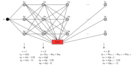
Figure 1: The construction of the function $f_{R}(\cdot)$ by a ReLU network, denoted as sub network 1 (Sub1).

Next, we approximate the function $xy=2^{-1}((x+y)^{2}-x^{2}-y^{2})$ for $x\in[0,1]$ and $y\in[0,1]$ by a ReLU network as follows. By the above results, we have $|f_{R}(\frac{x+y}{2})-(\frac{x+y}{2})^{2}|\leq 2^{-2R-2}$, $|2^{-2}f_{R}(x)-2^{-2}x^{2}|\leq 2^{-2}2^{-2R-2}$ and $|2^{-2}f_{R}(y)-2^{-2}y^{2}|\leq 2^{-2}2^{-2R-2}$. Let

$$\widetilde{f}_{R}(x,y)=2\left\{f_{R}(\frac{x+y}{2})-\frac{f_{R}(x)}{2^{2}}-\frac{f_{R}(y)}{2^{2}}\right\},$$

and $\widetilde{f}_{R}(x,y)$ can be implemented by a ReLU network having the depth, the computational units and the number of weights being $c_{1}R+c_{2}$, where the constants $c_{1}$ and $c_{2}$ can be different for these three measures. Moreover, $\widetilde{f}_{R}(x,y)=0$ if $xy=0$. For all $x\in[0,1]$ and $y\in[0,1]$,

$$\left|\widetilde{f}_{R}(x,y)-xy\right|=2\left|\left\{f_{R}(\frac{x+y}{2})-\frac{f_{R}(x)}{2^{2}}-\frac{f_{R}(y)}{2^{2}}\right\}-\left\{(\frac{x+y}{2})^{2}-\frac{x^{2}}{2^{2}}-\frac{y^{2}}{2^{2}}\right\}\right|$$

$$\leq 2\left(2^{-2R-2}+2^{-2}2^{-2R-2}+2^{-2}2^{-2R-2}\right)=3\cdot 2^{-2R-2}.$$ (4)

Figure 2 depicts the construction of $\widetilde{f}_{R}(x,y)$ from the Sub1’s, and we denote it as sub network 2 (Sub2).

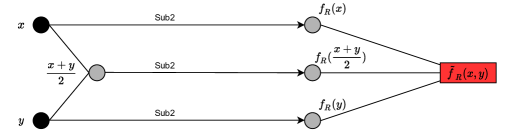
Figure 2: The construction of $\widetilde{f}_{R}(x,y)$ from the Sub1’s, we denote it as subnetwork 2 (Sub2).

If there are two covariates $\boldsymbol{X}=(X_{1},X_{2})^{\top}$, then $\phi_{\boldsymbol{\ell},\boldsymbol{s}}(\boldsymbol{x})=\phi_{\ell_{1},s_{1}}(x_{1})\phi_{\ell_{2},s_{2}}(x_{2})$ can be approximated by $\widetilde{f}_{R}(\phi_{\ell_{1},s_{1}}(x_{1}),\phi_{\ell_{2},s_{2}}(x_{2}))$. Next we approximate $\phi_{\boldsymbol{\ell},\boldsymbol{s}}(\boldsymbol{x})$ by a ReLU network from a binary tree structure for the general setting with $d$-dimensional covariates $\boldsymbol{X}=\mathbf{(}X_{1},\ldots,X_{d})^{\top}$. For notational simplicity, we denote $\digamma_{j_{1},...,j_{q}}=\phi_{\ell_{j_{1}},s_{j_{1}}}(x_{j_{1}})\times\cdot\cdot\cdot\times\phi_{\ell_{j_{q}},s_{j_{q}}}(x_{j_{q}})$ and $\widetilde{\digamma}_{j_{1},...,j_{q}j_{1}^{\prime},...,j_{p}^{\prime}}=\widetilde{f}_{R}(\digamma_{j_{1},...,j_{q}},\digamma_{j_{1}^{\prime},...,j_{p}^{\prime}})$. Then for any $1\leq j_{1}\neq j_{2}\leq d$, $\digamma_{j_{1}}\digamma_{j_{2}}=\phi_{\ell_{j_{1}},s_{j_{1}}}(x_{j_{1}})\phi_{\ell_{j_{2}},s_{j_{2}}}(x_{j_{2}})$ can be approximated by $\widetilde{\digamma}_{j_{1}j_{2}}=\widetilde{f}_{R}(\digamma_{j_{1}},\digamma_{j_{2}})$, and (4) leads to $|\widetilde{\digamma}_{j_{1}j_{2}}-\digamma_{j_{1}}\digamma_{j_{2}}|\leq 3\cdot 2^{-2R-2}$. Next, we approximate $\widetilde{\digamma}_{j_{1}j_{2}}\widetilde{\digamma}_{j_{3}j_{4}}$ with $\widetilde{\digamma}_{j_{1}j_{2}j_{3}j_{4}}=\widetilde{f}_{R}(\widetilde{\digamma}_{j_{1}j_{2}},\widetilde{\digamma}_{j_{3}j_{4}})$, and

$$|\widetilde{\digamma}_{j_{1}j_{2}j_{3}j_{4}}-\widetilde{\digamma}_{j_{1},j_{2}}\widetilde{\digamma}_{j_{3},j_{4}}|\leq 3\cdot 2^{-2R-2}.$$

These results lead to

$$|\widetilde{\digamma}_{j_{1}j_{2}}\widetilde{\digamma}_{j_{3}j_{4}}-\digamma_{j_{1}}\digamma_{j_{2}}\digamma_{j_{3}}\digamma_{j_{4}}| = |\widetilde{\digamma}_{j_{1}j_{2}}\widetilde{\digamma}_{j_{3}j_{4}}-\digamma_{j_{1}}\digamma_{j_{2}}\widetilde{\digamma}_{j_{3}j_{4}}+\digamma_{j_{1}}\digamma_{j_{2}}\widetilde{\digamma}_{j_{3}j_{4}}-\digamma_{j_{1}}\digamma_{j_{2}}\digamma_{j_{3}}\digamma_{j_{4}}|$$

$$\leq |\widetilde{\digamma}_{j_{1}j_{2}}-\digamma_{j_{1}}\digamma_{j_{2}}||\widetilde{\digamma}_{j_{3}j_{4}}|+|\digamma_{j_{1}}\digamma_{j_{2}}||\widetilde{\digamma}_{j_{3}j_{4}}-\digamma_{j_{3}}\digamma_{j_{4}}|$$

$$\leq 2\cdot 3\cdot 2^{-2R-2}.$$

Thus

$$|\widetilde{\digamma}_{j_{1}j_{2}j_{3}j_{4}}-\digamma_{j_{1}}\digamma_{j_{2}}\digamma_{j_{3}}\digamma_{j_{4}}| \leq |\widetilde{\digamma}_{j_{1}j_{2}j_{3}j_{4}}-\widetilde{\digamma}_{j_{1}j_{2}}\widetilde{\digamma}_{j_{3}j_{4}}|+|\widetilde{\digamma}_{j_{1}j_{2}}\widetilde{\digamma}_{j_{3}j_{4}}-\digamma_{j_{1}}\digamma_{j_{2}}\digamma_{j_{3}}\digamma_{j_{4}}|$$

$$\leq (1+2)\cdot 3\cdot 2^{-2R-2}.$$

By following the same argument, we have

$$|\widetilde{\digamma}_{j_{1}j_{2}j_{3}j_{4}j_{5}j_{6}j_{7}j_{8}}-\digamma_{j_{1}}\digamma_{j_{2}}\digamma_{j_{3}}\digamma_{j_{4}}\digamma_{j_{5}}\digamma_{j_{6}}\digamma_{j_{7}}\digamma_{j_{8}}|$$

$$\leq |\widetilde{\digamma}_{j_{1}\cdot\cdot\cdot j_{8}}-\widetilde{\digamma}_{j_{1}j_{2}j_{3}j_{4}}\widetilde{\digamma}_{j_{5}j_{6}j_{7}j_{8}}|+|\widetilde{\digamma}_{j_{1}j_{2}j_{3}j_{4}}-\digamma_{j_{1}}\digamma_{j_{2}}\digamma_{j_{3}}\digamma_{j_{4}}||\widetilde{\digamma}_{j_{5}j_{6}j_{7}j_{8}}|$$

$$+|\digamma_{j_{1}}\digamma_{j_{2}}\digamma_{j_{3}}\digamma_{j_{4}}||\widetilde{\digamma}_{j_{5}j_{6}j_{7}j_{8}}-\digamma_{j_{5}}\digamma_{j_{6}}\digamma_{j_{7}}\digamma_{j_{8}}|$$

$$\leq (1+2(1+2))\cdot 3\cdot 2^{-2R-2}=(1+2+2^{2})\cdot 3\cdot 2^{-2R-2}.$$

Define

$$\widetilde{\phi}_{\boldsymbol{\ell},\boldsymbol{s}}(\boldsymbol{x})=\widetilde{\digamma}_{1\cdot\cdot\cdot d}.$$

We continue the above process and it can be shown from mathematical induction (Montanelli and Du, 2019) that for all $\boldsymbol{x}\in\mathcal{X}$,

$$|\widetilde{\phi}_{\boldsymbol{\ell},\boldsymbol{s}}(\boldsymbol{x})-\phi_{\boldsymbol{\ell},\boldsymbol{s}}(\boldsymbol{x})|=|\widetilde{\digamma}_{1\cdot\cdot\cdot d}-\digamma_{1}\times\cdot\cdot\cdot\times\digamma_{d}|$$ (5)

$$\leq (1+2+2^{2}+\cdot\cdot\cdot+2^{\left\lfloor\log_{2}d\right\rfloor-1})\cdot 3\cdot 2^{-2R-2}\leq 3\cdot 2^{-2R-2}(d-1),$$

where $\left\lfloor a\right\rfloor$ is the largest integer no greater than $a$. Moreover, $\widetilde{\phi}_{\boldsymbol{\ell},\boldsymbol{s}}(\boldsymbol{x})=0$ if $\phi_{\boldsymbol{\ell},\boldsymbol{s}}(\boldsymbol{x})=0$. The ReLU network used to approximate $\phi_{\boldsymbol{\ell},\boldsymbol{s}}(\boldsymbol{x})$ has depth $\mathcal{O}(R)\times\log_{2}d=\mathcal{O}(R\log_{2}d)$, the computational units $\mathcal{O}(R)\times(d+2^{-1}d+\cdot\cdot\cdot+2^{-\left\lfloor\log_{2}d\right\rfloor+1}d)=\mathcal{O}(Rd)$, and the number of weights $\mathcal{O}(Rd)$. Figure 3 shows the construction of each approximated basis function approximator $\widetilde{\phi}_{\boldsymbol{\ell},\boldsymbol{s}}(\boldsymbol{x})$ from the Sub2’s, and we denote it as sub network 3 (Sub3).

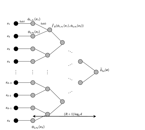
Figure 3: The construction of $\tilde{\phi}_{\boldsymbol{\ell},\boldsymbol{s}}(\boldsymbol{x})$ from the Sub2’s, we denote it as subnetwork 3 (Sub3).

Then the ReLU network approximator of the unknown function $f(\boldsymbol{x})$ is

$$\widetilde{f}_{R}(\boldsymbol{x})=\sum_{|\boldsymbol{\ell|}_{1}\leq m}\sum_{s\in I_{\boldsymbol{\ell}}}\gamma_{{}_{\boldsymbol{\ell},\boldsymbol{s}}}^{0}\widetilde{\phi}_{\boldsymbol{\ell},\boldsymbol{s}}(\boldsymbol{x})=\sum_{|\boldsymbol{\ell|}_{1}\leq m}\widetilde{g}_{\boldsymbol{\ell}}(\boldsymbol{x}).$$ (6)

Assumption 3.

Assume that for all $\boldsymbol{x}\in\mathcal{X}$, $0\leq\mu_{X}^{\prime}(\boldsymbol{x})\leq c_{\mu}$ for some constant $c_{\mu}\in(0,\infty)$.

The following proposition provides the approximation error of the approximator $\widetilde{f}_{R}\left(\cdot\right)$ obtained from the ReLU network to the true unknown function $f\left(\cdot\right)$.

Proposition 2.

For any $f\in W^{2,p}(\mathcal{X)}$, $2\leq p\leq\infty$, under Assumption 3, one has for $d=2,$

$$||\widetilde{f}_{R}-f||_{2}\leq\left\{\sqrt{\frac{3}{8}}2^{-2R}(d-1)(\sqrt{\frac{2}{3}})^{d-1}+9^{-1}c_{\mu}2^{-2m}(m+3)\right\}||D^{\boldsymbol{2}}f||_{L^{2}};$$

for $d\geq 3,$

$$||\widetilde{f}_{R}-f||_{2}\leq\left\{\sqrt{\frac{3}{8}}2^{-2R}(d-1)(\sqrt{\frac{2}{3}})^{d-1}+\widetilde{c}2^{-2m}\sqrt{d-2}\left(\frac{e}{3}\frac{m+d}{d-2}\right)^{d-1}\right\}||D^{\boldsymbol{2}}f||_{L^{2}},$$

where $\widetilde{c}=2^{-1}c_{\mu}(3\sqrt{2\pi}e)^{-1}$. The ReLU network that is used to construct the approximator $\widetilde{f}_{R}$ has depth $\mathcal{O}(R\log_{2}d)$, the number of computational units $\mathcal{O}(Rd)\times|V_{m}^{\left(1\right)}|=\mathcal{O}\left(2^{m}d^{3/2}R\left(m+d\right)^{-1}\left(4e\frac{m+d}{d-1}\right)^{{}^{d-1}}\right)$, and the number of weights $\mathcal{O}(Rd)\times|V_{m}^{\left(1\right)}|=\mathcal{O}\left(2^{m}d^{3/2}R\left(m+d\right)^{-1}\left(4e\frac{m+d}{d-1}\right)^{{}^{d-1}}\right)$.

Remark 4.

From Figure 3 and the mathematical expression (6), we see that the approximator $\widetilde{f}_{R}(\boldsymbol{\cdot})$ of the unknown function $f(\boldsymbol{\cdot})$ is constructed from a sparse deep ReLU network, as the nodes on each layer are not fully connected with the nodes from the previous layer, and the depth of the network has the order of $R\log_{2}d$ which increases with $R$.

Remark 5.

Montanelli and Du (2019) showed that the approximation error of the deep ReLU network can achieve accuracy $\epsilon>0$. We further derive an explicit form of the bound to see how it depends on the dimension and the network complexity. In Theorem 3, we will show that $m$ and $R$ need to grow with the sample size $n$ slowly at a logarithmic rate to achieve tradeoff between bias and variance, so the depth of the ReLU network grow with $n$ at a logarithmic rate, and the number of computational units increase with $n$ at a polynomial rate.

4 Sparse deep ReLU network estimator

In this section,  we will introduce the sparse deep ReLU network (SDRN) estimator of the unknown function $f_{0}$ obtained from (1). As discussed in Section 3, for $f_{0}\in W^{2,p}(\mathcal{X)}$, there exists a sparse deep ReLU approximator $\widetilde{f}_{R}(\boldsymbol{x})=\sum_{|\boldsymbol{\ell|}_{1}\leq m}\sum_{s\in I_{\boldsymbol{\ell}}}\gamma_{{}_{\boldsymbol{\ell},\boldsymbol{s}}}^{0}\widetilde{\phi}_{\boldsymbol{\ell},\boldsymbol{s}}(\boldsymbol{x})$, where the expression of $\gamma_{{}_{\boldsymbol{\ell},\boldsymbol{s}}}^{0}$ is given in (A.2), which has the approximation error given in Theorem 2 with $f\left(\cdot\right)$ replaced by the true target function $f_{0}\left(\cdot\right)$ in (1).

Define the ReLU network class as

$$\mathcal{F(}\widetilde{\phi},m,B)=\{f_{RL}:\mathcal{X}\rightarrow\mathbb{R},f_{RL}(\boldsymbol{x})=\sum_{|\boldsymbol{\ell|}_{1}\leq m}\sum_{s\in I_{\boldsymbol{\ell}}}\gamma_{{}_{\boldsymbol{\ell},\boldsymbol{s}}}\widetilde{\phi}_{\boldsymbol{\ell},\boldsymbol{s}}(\boldsymbol{x}),\eta_{{}_{\boldsymbol{\ell},\boldsymbol{s}}}\in\mathbb{R},||f_{RL}||_{\infty}\leq B\},$$ (7)

with $B\geq\max(||f_{0}||_{\infty},||\widetilde{f}_{R}||_{\infty})$. Then $\widetilde{f}_{R}\in\mathcal{F(}\widetilde{\phi},m,B)$. Denote $\boldsymbol{\gamma}=\{\gamma_{{}_{\boldsymbol{\ell},\boldsymbol{s}}}:s\in I_{\boldsymbol{\ell}},|\boldsymbol{\ell|}_{1}\leq m\}^{\top}$ and $\widetilde{\phi}(\boldsymbol{x})=\{\widetilde{\phi}_{\boldsymbol{\ell},\boldsymbol{s}}(\boldsymbol{x}):s\in I_{\boldsymbol{\ell}},|\boldsymbol{\ell|}_{1}\leq m\}^{\top}$, $f_{RL}(\boldsymbol{x})$ can be written as $f_{RL}(\boldsymbol{x})=\widetilde{\phi}(\boldsymbol{x})^{\top}\boldsymbol{\gamma}$. We obtain the unpenalized SDRN estimator $\widehat{f}_{RL}^{U}$ of $f_{0}$ from minimizing the following empirical risk:

$$\widehat{f}_{RL}^{U}=\arg\min_{f_{RL}\in\mathcal{F(}\widetilde{\phi},m,B)}\mathcal{E}_{n}(f_{RL})\text{, where }\mathcal{E}_{n}(f_{RL})=n^{-1}\sum_{i=1}^{n}\rho(f_{RL}(\boldsymbol{X}_{i}),Y_{i}).$$ (8)

Similarly, we can also obtain the penalized SDRN estimator $\widehat{f}_{RL}^{P}$ of $f_{0}$ from minimizing

$$\widehat{f}_{RL}^{P}=\arg\min_{f_{RL}\in\mathcal{F(}\widetilde{\phi},m,B)}\{\mathcal{E}_{n}(f_{RL})+2^{-1}\lambda||f_{RL}||_{\Psi}^{2}\},$$

where $\lambda>0$ is a tuning parameter for the $L_{2}$ penalty, and $||f_{RL}||_{\Psi}^{2}=\boldsymbol{\gamma}^{\top}\left[\int\{\widetilde{\phi}(\boldsymbol{x})\widetilde{\phi}(\boldsymbol{x})^{\top}\}d\boldsymbol{x}\right]\Psi\boldsymbol{\gamma}$. The $L_{2}$ penalty is often used to prevent overfitting. Here, we let $\Psi=\left[\int\{\widetilde{\phi}(\boldsymbol{x})\widetilde{\phi}(\boldsymbol{x})^{\top}\}d\boldsymbol{x}\right]^{-1}$, so that $||f_{RL}||_{\Psi}^{2}=\boldsymbol{\gamma}^{\top}\boldsymbol{\gamma}$.

We use $\widehat{f}_{RL}$ as a generic notation for a SDRN estimator; it can be either the unpenalized or the penalized estimator. For a given estimator $\widehat{f}_{RL}$, we define the overall error as $\mathcal{E}(\widehat{f}_{RL})-\mathcal{E}(f_{0})$, which is used to measure how close the estimator $\widehat{f}_{RL}$ to the true target function $f_{0}$. Let

$$f_{RL}^{0}=\arg\min_{f_{RL}\in\mathcal{F(}\widetilde{\phi},m,B)}\mathcal{E}(f_{RL})\text{, where }\mathcal{E}(f_{RL})=\int_{\mathcal{X\times Y}}\rho(f_{RL}(\boldsymbol{x}),y)d\mu(\boldsymbol{x,}y).$$ (9)

Then the overall error of the estimator $\widehat{f}_{RL}$ can be splitted into the approximation error $\mathcal{E}(f_{RL}^{0})-\mathcal{E}(f_{0})$ and the sampling error $\mathcal{E}(\widehat{f}_{RL})-\mathcal{E}(f_{RL}^{0})$ such that

$$\underset{\text{overall error}}{\underbrace{\mathcal{E}(\widehat{f}_{RL})-\mathcal{E}(f_{0})}}=\underset{\text{approximation error}}{\underbrace{\mathcal{E}(f_{RL}^{0})-\mathcal{E}(f_{0})}}+\underset{\text{estimation error}}{\underbrace{\mathcal{E}(\widehat{f}_{RL})-\mathcal{E}(f_{RL}^{0})}}.$$

We will establish the upper bounds for the approximation error and the estimation error, respectively, as follows.

We introduce the following Bernstein condition that is required for obtaining the probability bound for the estimation error of our SDRN estimator.

Assumption 4.

There exists a constant $0<a_{\rho}<\infty$ such that

$$a_{\rho}||f-f_{RL}^{0}||_{2}^{2}\leq\mathcal{E}(f)-\mathcal{E}(f_{RL}^{0})$$ (10)

for any $f\in\mathcal{F(}\widetilde{\phi},m,B)$.

Remark 6.

The Bernstein condition given in (10) for Lipschitz loss functions is used in the literature in order to establish probability bounds of estimators obtained from empirical risk minimization (Alquier et al, 2019). A more general form is $a_{\rho}||f-f_{RL}^{0}||_{2}^{2\kappa}\leq\mathcal{E}(f)-\mathcal{E}(f_{RL}^{0})$ for some $\kappa\geq 1$. The parameter $\kappa$ can affect the estimator’s rate of convergence. For proof convenience, we let $\kappa=1$ which is satisfied by many commonly used loss functions. We will give a detailed discussion on this Bernstein condition, and will present different examples in Section 5 of the Appendix.

Remark 7.

From the Lipschitz condition given in Assumption 2, we have that there exists a constant $0<M_{\rho}<\infty$ such that $|\rho\left(f(\boldsymbol{x}),y\right)|\leq M_{\rho}$, for almost every $(\boldsymbol{x},y)\in\mathcal{X}\times\mathcal{Y}$ and any $f\in\mathcal{F(}\widetilde{\phi},m,B)$.

Another condition is given below and it is used for controlling the approximation error from the ReLU networks.

Assumption 5.

There exists a constant $0<b_{\rho}<\infty$ such that

$$\mathcal{E}(f)-\mathcal{E}(f_{0})\leq b_{\rho}||f-f_{0}||_{2}^{2}$$ (11)

for any $f\in\mathcal{F(}\widetilde{\phi},m,B)$.

Remark 8.

Assumption 5 is introduced for controlling the approximation error $\mathcal{E}(f_{RL}^{0})-\mathcal{E}(f_{0})$, but it is not required for establishing the upper bound of the sampling error $\mathcal{E}(\widehat{f}_{RL})-\mathcal{E}(f_{RL}^{0})$. The approximation error $\mathcal{E}(f_{RL}^{0})-\mathcal{E}(f_{0})$ can be well controlled based on the result from Proposition 2 together with Assumption 5. Without this assumption, the approximation error will have a slower rate. Assumption 5 is satisfied by the quadratic, logistic, quantile and Huber loss functions under mild conditions. More discussions on this assumption will be provided in Section 5 of the Appendix.

Under Condition (11) given in Assumption 5, by the definition of $f_{RN}^{0}$ given in (9) and Proposition 2, the approximation error

$$\mathcal{E}(f_{RN}^{0})-\mathcal{E}(f_{0})\leq\mathcal{E}(\widetilde{f}_{R})-\mathcal{E}(f_{0})\leq b_{\rho}||\widetilde{f}_{R}-f_{0}||_{2}^{2}.$$

Since $f_{0}$ satisfies Assumption 1, then $||D^{\boldsymbol{2}}f_{0}||_{L^{2}}\leq C_{f}$ for some constant $C_{f}\in(0,\infty)$. Next proposition presents an upper bound for the approximation error when the unknown function $f_{0}$ is approximated by the SDRN obtained from the ERM in (9).

Proposition 3.

Under Assumptions 1, 3 and 5, and $m^{-1}=o(1)$ and $m\lesssim R$, one has

$$\mathcal{E}(f_{RN}^{0})-\mathcal{E}(f_{0})\leq\zeta_{R,m,d},$$

where

$$\zeta_{R,m,d} = 4b_{\rho}C_{f}^{2}\widetilde{c}^{2}2^{-4m}d\left(\frac{e}{3}\frac{m+d}{d-2}\right)^{2\left(d-1\right)},\text{ for }d\geq 3$$

$$\zeta_{R,m,d} = 81^{-1}b_{\rho}C_{f}^{2}c_{\mu}^{2}2^{-4m}(m+3)^{2},\text{ for }d=2.$$ (12)

Note that without Assumption 5, we obtain a looser bound for $\mathcal{E}(f_{RL}^{0})-\mathcal{E}(f_{0})=\mathcal{O(}\zeta_{R,m,d}^{1/2})$ based on the result $\mathcal{E}(\widetilde{f}_{R})-\mathcal{E}(f_{0})\leq C_{\rho}||\widetilde{f}_{R}-f_{0}||_{2}$ which is directly implied from Assumption 2.

Next we establish the bound for the sampling error $\mathcal{E}(\widehat{f}_{RL})-\mathcal{E}(f_{RL}^{0})$. Let $\mathcal{N}(\delta,\mathcal{F},||\cdot||_{\infty})$ be the covering number, that is, the minimal number of $||\cdot||_{\infty}$- balls with radius $\delta$ that covers $\mathcal{F}$ and whose centers reside in $\mathcal{F}$. Let $\lambda_{\min,\widetilde{\phi}}=\lambda_{\min}\left\{\int\widetilde{\phi}(\boldsymbol{x})\widetilde{\phi}(\boldsymbol{x})^{\top}d\mu_{X}(\boldsymbol{x})\right\}$. In the theorem below, we provide an upper bound for the estimation error $\mathcal{E}(\widehat{f}_{RL})-\mathcal{E}(f_{RL}^{0})$.

Theorem 1.

Under Assumptions 1-4, we have that for any $\epsilon>0$, i)

$$P\left(\mathcal{E}(\widehat{f}_{RL}^{U})-\mathcal{E}(f_{RL}^{0})>\epsilon\right)\leq\mathcal{N}(\sqrt{2}C_{\rho}^{-1}\epsilon/8,\mathcal{F(}\widetilde{\phi},m,B),||\cdot||_{\infty})\exp\left(-n\epsilon/C^{\ast}\right),$$

and ii) with $\lambda\lambda_{\min,\widetilde{\phi}}^{-1}\leq 5^{-1}a_{\rho}^{1/2}\min(a_{\rho}^{1/2},B\sqrt{\epsilon/2})$,

$$P\left\{\mathcal{E}(\widehat{f}_{RL}^{P})-\mathcal{E}(f_{RL}^{0})>2\epsilon\right\}\leq\mathcal{N}(\sqrt{2}C_{\rho}^{-1}\epsilon/8,\mathcal{F(}\widetilde{\phi},m,B),||\cdot||_{\infty})\exp\left(-n\epsilon/C^{\ast}\right),$$

where $C^{\ast}=64(C_{\rho}^{2}a_{\rho}^{-1}+4M_{\rho}/3)$, in which $C_{\rho},a_{\rho}$ and $M_{\rho}$ are constants given in Assumptions 2 and 4 and Remark 7.

Remark 9.

Let $c^{\prime}=1$ if $\widehat{f}_{RL}=\widehat{f}_{RL}^{U}$ and $c^{\prime}=2$ if $\widehat{f}_{RL}=\widehat{f}_{RL}^{P}$. The two probability bounds established in Theorem 1 can be summarized as

$$P\left\{\mathcal{E}(\widehat{f}_{RL})-\mathcal{E}(f_{RL}^{0})>c^{\prime}\epsilon\right\}\leq\mathcal{N}(\sqrt{2}C_{\rho}^{-1}\epsilon/8,\mathcal{F(}\widetilde{\phi},m,B),||\cdot||_{\infty})\exp\left(-n\epsilon/C^{\ast}\right),$$

where $\widehat{f}_{RL}$ can be both the unpenalized and penalized estimators.

Theorem 2.

Under the same assumptions as given in Theorem 1,

$$P\left(\mathcal{E}(\widehat{f}_{RL})-\mathcal{E}(f_{RL}^{0})>c^{\prime}\frac{C^{\ast}|V_{m}^{\left(1\right)}|}{n}\max(1,\log\frac{C^{\ast\ast}n}{|V_{m}^{\left(1\right)}|\varsigma})\right)\leq\varsigma,$$

where $c^{\prime}=1$ if $\widehat{f}_{RL}=\widehat{f}_{RL}^{U}$ and $c^{\prime}=2$ if $\widehat{f}_{RL}=\widehat{f}_{RL}^{P}$, $C^{\ast}$ is given in Theorem 1, $C^{\ast\ast}=12C_{\rho}B/C^{\ast}$ and $\varsigma=(\frac{C^{\ast\ast}C^{\ast}}{\epsilon})^{|V_{m}^{\left(1\right)}|}\exp\left(-n\epsilon/C^{\ast}\right)$, for any $\epsilon\in(0,C_{\rho}B/2)$.

Based on the upper bound for the estimation error given in Theorem 2, and the bound for the approximation error given in (12), we can further obtain the risk rate of the SDRN estimator $\widehat{f}_{RL}$ presented in the following theorems.

Theorem 3.

Under Assumptions 1-5, $2^{m}\asymp n^{1/5}$ and $m\lesssim R$, if (i) $d\asymp(\log_{2}n)^{\kappa}$ for some constant $\kappa\in(0,1)$, then $\mathcal{E}(f_{RN}^{0})-\mathcal{E}(f_{0})=o(n^{-4/5+\varpi}(\log_{2}n)^{3\kappa-2})$ and $\mathcal{E}(\widehat{f}_{RN})-\mathcal{E}(f_{RN}^{0})=\mathcal{O}_{p}(n^{-4/5+\varpi/2}(\log_{2}n)^{3\kappa/2})$, for an arbitrarily small $\varpi>0$. Thus

$$\mathcal{E}(\widehat{f}_{RN})-\mathcal{E}(f_{0})=o_{p}(n^{-4/5+\varpi}(\log_{2}n)^{3\kappa-2}).$$

The above rate is satisfied by both $\widehat{f}_{RN}^{U}$ and $\widehat{f}_{RN}^{P}$ with $\lambda=\mathcal{O}(\lambda_{\min,\widetilde{\phi}}n^{-2/5+\varpi/4}(\log_{2}n)^{3\kappa/4})$.

If $R\asymp\log_{2}n$, the ReLU network that is used to construct the estimator $\widehat{f}_{RN}$ has depth $\mathcal{O}[\log_{2}n\{\log_{2}(\log_{2}n)\}]$, the number of computational units $\mathcal{O}\{\left(\log_{2}n\right)^{5\kappa/2-1}n^{1/5+\varpi/2}\}$, and the number of weights $\mathcal{O}\{\left(\log_{2}n\right)^{5\kappa/2-1}n^{1/5+\varpi/2}\}$.

If (ii) $d\asymp 1$, then $\mathcal{E}(f_{RN}^{0})-\mathcal{E}(f_{0})=\mathcal{O}(n^{-4/5}(d^{-1}\log_{2}n)^{2d-2})$ and $\mathcal{E}(\widehat{f}_{RN})-\mathcal{E}(f_{RN}^{0})=\mathcal{O}_{p}(n^{-4/5}(d^{-1}\log_{2}n)^{d})$. Thus

$$\mathcal{E}(\widehat{f}_{RN})-\mathcal{E}(f_{0})=\mathcal{O}_{p}(n^{-4/5}(d^{-1}\log_{2}n)^{2d-2}).$$

The above rate is satisfied by both $\widehat{f}_{RN}^{U}$ and $\widehat{f}_{RN}^{P}$ with $\lambda=\mathcal{O}(\lambda_{\min,\widetilde{\phi}}n^{-2/5}(d^{-1}\log_{2}n)^{d/2})$.

If $R\asymp\log_{2}n$, the ReLU network that is used to construct the estimator $\widehat{f}_{RN}$ has depth $\mathcal{O}(\log_{2}n)$, the number of computational units $\mathcal{O}\{\left(\log_{2}n\right)^{d-1}n^{1/5}\}$, and the number of weights $\mathcal{O}\{\left(\log_{2}n\right)^{d-1}n^{1/5}\}$.

Remark 10.

Note that Assumption 5 is not required for obtaining the convergence rate of the sampling error $\mathcal{E}(\widehat{f}_{RN})-\mathcal{E}(f_{RN}^{0})$, it is only needed for the rate of the approximation error $\mathcal{E}(f_{RN}^{0})-\mathcal{E}(f_{0})$. Without this assumption, the rate of $\mathcal{E}(f_{RN}^{0})-\mathcal{E}(f_{0})$ is slower.

Remark 11.

The risk rates in Theorem 3 are summarized as $\mathcal{E}(\widehat{f}_{RN})-\mathcal{E}(f_{0})=o_{p}(n^{-4/5+\varpi}(\log_{2}n)^{3\kappa-2})$ if $d\asymp(\log_{2}n)^{\kappa}$ and $\mathcal{E}(\widehat{f}_{RN})-\mathcal{E}(f_{0})=\mathcal{O}_{p}(n^{-4/5}(d^{-1}\log_{2}n)^{2d-2})$ if $d\asymp 1$.

Remark 12.

We focus on deriving the optimal risk rate for the SDRN estimator of the unknown function $f_{0}$ when it belongs to the Korobov space of mixed derivatives of order $\beta=2$. Then the derived rate can be written as $n^{-2\beta/(2\beta+1)}(d^{-1}\log_{2}n)^{2d-2}$ when $d$ is fixed. It is possible to derive a similar estimator for a smoother regression function that has mixed derivatives of order $\beta>2$ when Jacobi-weighted Korobov spaces (Shen and Wang, 2010) are considered. This can be an interesting topic for future work.

Remark 13.

It is worth noting that for the classical nonparametric regression estimators such as spline estimators (Stone, 1982), the optimal minimax risk rate is $n^{-4/(4+d)}$, if the regression function belongs to the Sobolev spaces $S^{2,p}(\mathcal{X})$. This rate suffers from the curse of dimensionality as $d$ increases. For one-dimensional nonparametric regression with $d=1$, the optimal rate becomes $n^{-4/5}$.

Bauer and Kohler (2019) showed that their least squares neural network estimator can achieve the rate $n^{-2\beta/(2\beta+d^{\ast})}$ (up to a log factor), if the regression function satisfies a $\beta$-smooth generalized hierarchical interaction model of order $d^{\ast}$. When $\beta=2$, the rate is $n^{-4/(4+d^{\ast})}$. The rates mentioned above require $d$ to be fixed. Bauer and Kohler (2019) consider a smooth activation function, while Schmidt-Hieber (2020) established a similar optimal rate for ReLU activation function.

Theorem 3 shows that when $f_{0}$ belongs to the Korobov spaces $W^{2,p}(\mathcal{X)}$, our SDRN estimator has the risk rate $n^{-4/5}(d^{-1}\log_{2}n)^{2d-2}$ and it achieves the optimal minimax rate (up to a log factor) as one-dimensional nonparametric regression, if the dimension $d$ is fixed. The effect of $d$ is passed on to a logarithm order, so the curse of dimensionality can be alleviated. When $d$ increases with $n$ with an order $(\log_{2}n)^{\kappa}$, the risk rate is slightly slower than $n^{-4/5}$.

5 Discussions on Assumptions 4 and 5

We first state a general condition given in Assumption 6 presented below. We will show that if a loss function satisfies this condition, then it will satisfy Assumption 4 (Bernstein condition) and Assumption 5.

Assumption 6.

For all $y\in\mathcal{Y}$, the loss function $\rho\left(\cdot,y\right)$ is strictly convex and it has a bounded second derivative such that $\rho^{\prime\prime}\left(\cdot,y\right)\in[2a_{\rho},2b_{\rho}]$ almost everywhere, for some constants $0<a_{\rho}\leq b_{\rho}<\infty$.

Assumption 6 is satisfied by a variety of classical loss functions such as quadratic loss and logistic loss. For example, for the quadratic loss $\rho\left(f(\boldsymbol{x}),y\right)=(y-f(\boldsymbol{x}))^{2}$, clearly $\rho^{\prime\prime}\left(\cdot,y\right)=2$, so $a_{\rho}=b_{\rho}=1$.

Let $f_{{}_{0}}$ solve $\int_{\mathcal{Y}}\rho^{\prime}(f_{0}(\boldsymbol{x}),y)d\mu(y|\boldsymbol{x})=0$ and $f_{0}\in W^{2,p}(\mathcal{X})$. Then $f_{{}_{0}}$ is the target function that minimizes the expected risk given in (1). Lemma 1 given below will show that Assumptions 4 and 5 are implied from Assumption 6.

Lemma 1.

Under Assumption 6, for any $f\in\mathcal{F(}\widetilde{\phi},m,B)$, one has $a_{\rho}||f-f_{RL}^{0}||_{2}^{2}\leq\mathcal{E}(f)-\mathcal{E}(f_{RL}^{0})$ and $\mathcal{E}(f)-\mathcal{E}(f_{0})\leq b_{\rho}||f-f_{0}||_{2}^{2}$.

It is easy to see that the quantile and Huber loss functions do not satisfy Assumption 6. In the lemmas below we will show that under mild conditions, Assumptions 4 and 5 are satisfied by the quantile and Huber loss functions.

Lemma 2.

Assume that for all $\boldsymbol{x}\in\mathcal{X}$, it is possible to define a conditional density function of $Y|\boldsymbol{X}=\boldsymbol{x}$ such that $1/C_{1}\leq\mu^{\prime}(u|\boldsymbol{x})\leq 1/C_{2}$ for some $C_{1}\geq C_{2}>0$ for all $u\in\{u\in\mathbb{R}$: $|u-f_{RL}^{0}(\boldsymbol{x})|\leq 2B$ or $|u-f_{0}(\boldsymbol{x})|\leq 2B\}$. Then for any $f\in\mathcal{F(}\widetilde{\phi},m,B)$, the quantile loss given in (3) satisfies $a_{\rho}||f-f_{RL}^{0}||_{2}^{2}\leq\mathcal{E}(f)-\mathcal{E}(f_{RL}^{0})$ and $\mathcal{E}(f)-\mathcal{E}(f_{0})\leq b_{\rho}||f-f_{0}||_{2}^{2}$ with $a_{\rho}=(2C_{1})^{-1}$ and $b_{\rho}=(2C_{2})^{-1}$.

Lemma 3.

Assume that for all $\boldsymbol{x}\in\mathcal{X}$, $1/c_{1}\leq\mu(u+\delta|\boldsymbol{x})-\mu(u-\delta|\boldsymbol{x})\leq 1/c_{2}$ for some $c_{1}\geq c_{2}>0$ for all $u\in\{u\in\mathbb{R}$: $|u-f_{RL}^{0}(\boldsymbol{x})|\leq 2B$ or $|u-f_{0}(\boldsymbol{x})|\leq 2B\}$, where $\mu(u|\boldsymbol{x})$ is the conditonal cumulative function of $Y$ given $Y|\boldsymbol{X}=\boldsymbol{x}$. Then for any $f\in\mathcal{F(}\widetilde{\phi},m,B)$, the Huber loss given in (2) satisfies $a_{\rho}||f-f_{RL}^{0}||_{2}^{2}\leq\mathcal{E}(f)-\mathcal{E}(f_{RL}^{0})$ and $\mathcal{E}(f)-\mathcal{E}(f_{0})\leq b_{\rho}||f-f_{0}||_{2}^{2}$ with $a_{\rho}=(2c_{1})^{-1}$ and $b_{\rho}=(2c_{2})^{-1}$.

The proofs of Lemmas 1-3 are provided in Section A.9 of the Appendix.

6 Simulation studies

In this section, we conduct simulation studies to assess the finite-sample performance of the proposed methods.

6.1 Date generating process

For illustration of the methods, we generate data from the following nonlinear models:

Model 1 $$:\mathbb{E}(Y_{i}|X_{i})=X_{i1}^{2}+X_{i2}^{2}+1.5\sin(\sqrt{1.5}\pi(X_{i1}+X_{i2}))+\frac{X_{i3}}{X_{i1}^{2}+X_{i2}^{2}+1}+1;\text{ }X_{i}\sim\mathcal{U}\left([0,1]^{5}\right);$$

Model 2 $$:\mathbb{E}(Y_{i}|X_{i})=X_{i1}X_{i2}+\frac{e^{\sin(2\pi(X_{i3}+X_{i4}))}}{1+e^{\cos(2\pi X_{i5})}}+\tan(\frac{X_{i1}}{X_{i2}^{2}+X_{i4}^{4}+2});\text{ }X_{i}\sim\mathcal{U}\left([0,1]^{7}\right);$$

Model 3 $$:\mathbb{E}(Y_{i}|X_{i})=1.5X_{i5}{\cos(X_{i1}X_{i2}+X_{i3}+X_{i4})}+X_{i3}^{2}X_{i7}\sqrt{X_{i6}X_{i8}+X_{i9}+0.1}+\frac{2X_{i7}}{2+X_{i5}^{2}+X_{i10}^{4}}+1;$$

$$\text{ }X_{i}\sim\mathcal{U}\left([0,1]^{10}\right);$$

Model 4 $$:\mathbb{E}(Y_{i}|X_{i})=\mathbb{P}(Y_{i}=1|X_{i})=\frac{e^{\mu_{i}}}{1+e^{\mu_{i}}};$$

$$\mu_{i}=X_{i5}{\cos(X_{i1}X_{i2}+X_{i3}+X_{i4})}+X_{i3}^{2}X_{i7}\sqrt{X_{i6}X_{i8}+X_{i9}+0.1}+\frac{X_{i7}}{2+X_{i5}^{2}+X_{i10}^{4}}-3X_{i5}+1;$$

$$\text{ }X_{i}\sim\mathcal{U}\left([0,1]^{10}\right);$$

For Models 1-3, we generate the responses from $Y_{i}=E(Y_{i}\mid X_{i})+\epsilon_{i}$, and $\epsilon_{i}$ are independently generated from the standard normal distribution and Laplace distribution, respectively, for $1\leq i\leq n$. For each setting, we run $n_{rep}=100$ replications. For the SDRN estimator, we use $m=\max(\left\lfloor 0.2\log_{2}n\right\rfloor+c,0)$ and $R=3\max(\left\lfloor 0.2\log_{2}n\right\rfloor,m)$, which satisfy the conditions in Theorem 3, for different choices of $c$. Let the tuning parameter for the ridge penalty be $\lambda=\kappa n^{-1}$.

For Models 1-3, we evaluate the estimated function based on the same set of the covariate values $x_{i}^{\ast}(1\leq i\leq n)$, which are independently generated from $\mathcal{U}\left([0,1]^{p}\right)$. Let $\widehat{f}(x_{i}^{\ast})$ be the estimate of the target function $f(x_{i}^{\ast})$. We report

$$\text{average bias}^{2} = \frac{1}{n}\sum\nolimits_{i=1}^{n}\{\frac{1}{n_{rep}}\sum\nolimits_{j=1}^{n_{rep}}\widehat{f}(x_{i}^{\ast})-f(x_{i}^{\ast})\}^{2},$$

average variance $$= \frac{1}{n}\sum\nolimits_{i=1}^{n}\{\frac{1}{n_{rep}}\sum\nolimits_{j=1}^{n_{rep}}\widehat{f}(x_{i}^{\ast})^{2}-(\frac{1}{n_{rep}}\sum\nolimits_{j=1}^{n_{rep}}\widehat{f}(x_{i}^{\ast}))^{2}\},$$

average mse = $$\frac{1}{n}\sum\nolimits_{i=1}^{n}\frac{1}{n_{rep}}\sum\nolimits_{j=1}^{n_{rep}}\{\widehat{f}(x_{i}^{\ast})-f(x_{i}^{\ast})\}^{2}.$$

6.2 Simulation results

Tables 1 and 2 report the average mean squared error (MSE), average $\text{bias}^{2}$ and average variance the SDRN estimators obtained from the quadratic and quantile $(\tau=0.5,\ 0.25)$ loss functions for Model 1 when $n=2000,5000$. We let $\kappa$ equal 0.1, 0.5, 1, 2, 4 and $c$ equal -2, -1, 0, 1, 2, respectively. From Table 1 with $n=2000$, we observe that when the value of $\kappa$ is fixed, the increase of the $c$ value results in an overall trend of decreasing bias² and increasing variance. When $c$ is too small (for example, $c=-2$), the estimator can have a large bias due to possible underfitting. For a larger value of $c$, it correspondingly needs a larger value of $\kappa$ for the ridge penalty to prevent overfitting. A good choice of $(\kappa,\ c)$ leads to an optimal fitting with the smallest MSE. The smallest MSE value for each case is highlighted in bold and red, corresponding to the optimal fitting. We see that the estimate with the smallest MSE for each case achieves a good balance between the bias² and variance. Moreover, when the error is generated from the Laplace distribution, the estimate from the quantile $(\tau=0.5)$ loss, which is a robust estimate, has smaller MSE compared to that obtained from the quadratic loss. Table 2 shows the results for $n=5000$. We observe similar patterns as Table 1. Clearly, when $n$ increases, the MSE values become smaller. This corroborates our convergence results in Theorem 3. Tables A.9 and A.10 in the Appendix show the average MSE, average $\text{bias}^{2}$ and average variance for Model 2 when $n=2000,5000$. The results in Model 2 show similar pattens as those observed from Table 1 for Model 1.

Table 1: The average MSE, $\text{bias}^{2}$ and variance of the SDRN estimators obtained from the quadratic and quantile $\left(\tau=0.5,\ 0.25\right)$ loss functions based on the 100 simulation replications when $n=2000$ for Model 1.

		quadratic					quantile ($\tau=0.5)$					quantile ($\tau=0.25)$
$\kappa$		$c=-2$	$c=-1$	$c=0$	$c=1$	$c=2$	$c=-2$	$c=-1$	$c=0$	$c=1$	$c=2$	$c=-2$	$c=-1$	$c=0$	$c=1$	$c=2$
		Normal	error
$0.1$	bias2	0.4970	0.0879	0.0206	0.0096	0.0146	0.5036	0.0932	0.0258	0.0120	0.0143	0.5723	0.0949	0.0265	0.0190	0.0681
	var	0.0235	0.0504	0.1331	0.3420	0.7154	0.0301	0.0530	0.1300	0.3031	0.6141	0.0367	0.0604	0.1415	0.3069	0.5728
	mse	0.5205	0.1383	0.1538	0.3516	0.7300	0.5336	0.1463	0.1558	0.3151	0.6283	0.6090	0.1553	0.1680	0.3259	0.6408
$0.5$	bias2	0.5019	0.1046	0.0341	0.0178	0.0194	0.5303	0.1563	0.0582	0.0299	0.0253	0.6317	0.1714	0.0607	0.0291	0.0321
	var	0.0181	0.0328	0.0746	0.1594	0.2975	0.0179	0.0304	0.0633	0.1285	0.2450	0.0192	0.0331	0.0667	0.1297	0.2334
	mse	0.5199	0.1375	0.1087	0.1772	0.3169	0.5483	0.1867	0.1215	0.1584	0.2703	0.6509	0.2046	0.1274	0.1588	0.2655
$1$	bias2	0.5100	0.1347	0.0498	0.0273	0.0262	0.5718	0.2449	0.0998	0.0520	0.0405	0.6922	0.2805	0.1078	0.0522	0.0402
	var	0.0146	0.0257	0.0544	0.1101	0.1997	0.0126	0.0229	0.0439	0.0848	0.1540	0.0126	0.0238	0.0452	0.0850	0.1506
	mse	0.5246	0.1604	0.1042	0.1374	0.2259	0.5843	0.2678	0.1436	0.1369	0.1945	0.7048	0.3044	0.1530	0.1372	0.1907
$2$	bias2	0.5301	0.1980	0.0811	0.0448	0.0387	0.6567	0.3917	0.1792	0.0949	0.0695	0.7878	0.4587	0.2013	0.1007	0.0685
	var	0.0110	0.0195	0.0384	0.0741	0.1314	0.0080	0.0166	0.0296	0.0545	0.0964	0.0075	0.0160	0.0298	0.0541	0.0934
	mse	0.5411	0.2175	0.1195	0.1189	0.1701	0.6647	0.4083	0.2088	0.1495	0.1658	0.7954	0.4747	0.2311	0.1547	0.1620
$4$	bias2	0.5766	0.3063	0.1395	0.0769	0.0610	0.8157	0.5864	0.3171	0.1776	0.1245	0.9401	0.6628	0.3666	0.1969	0.1290
	var	0.0076	0.0144	0.0264	0.0487	0.0845	0.0046	0.0111	0.0194	0.0343	0.0590	0.0040	0.0098	0.0186	0.0333	0.0577
	mse	0.5843	0.3207	0.1659	0.1256	0.1456	0.8203	0.5975	0.3365	0.2119	0.1834	0.9441	0.6727	0.3851	0.2303	0.1867
		Laplace	error
$0.1$	bias2	0.4989	0.0894	0.0225	0.0131	0.0220	0.5079	0.0940	0.0273	0.0136	0.0176	0.5950	0.1035	0.0308	0.0136	0.0369
	var	0.0370	0.0948	0.2634	0.6866	1.4377	0.0327	0.0560	0.1388	0.3628	0.8235	0.0443	0.0851	0.2007	0.4450	0.8621
	mse	0.5359	0.1842	0.2859	0.6998	1.4597	0.5406	0.1501	0.1661	0.3764	0.8411	0.6393	0.1886	0.2315	0.4586	0.8990
$0.5$	bias2	0.5037	0.1068	0.0362	0.0195	0.0230	0.5370	0.1600	0.0613	0.0328	0.0287	0.6609	0.2065	0.0767	0.0361	0.0290
	var	0.0285	0.0611	0.1446	0.3141	0.5887	0.0192	0.0329	0.0646	0.1356	0.2757	0.0226	0.0470	0.0926	0.1785	0.3214
	mse	0.5322	0.1679	0.1807	0.3337	0.6118	0.5562	0.1929	0.1259	0.1684	0.3044	0.6834	0.2535	0.1693	0.2147	0.3504
$1$	bias2	0.5117	0.1373	0.0521	0.0290	0.0291	0.5809	0.2552	0.1050	0.0559	0.0444	0.7295	0.3370	0.1361	0.0668	0.0462
	var	0.0231	0.0471	0.1040	0.2144	0.3914	0.0133	0.0255	0.0448	0.0866	0.1641	0.0146	0.0323	0.0622	0.1160	0.2030
	mse	0.5348	0.1844	0.1561	0.2434	0.4205	0.5942	0.2806	0.1498	0.1425	0.2085	0.7440	0.3693	0.1982	0.1828	0.2492
$2$	bias2	0.5316	0.2012	0.0839	0.0468	0.0410	0.6705	0.4119	0.1883	0.1006	0.0745	0.8384	0.5216	0.2493	0.1281	0.0850
	var	0.0174	0.0349	0.0720	0.1422	0.2546	0.0085	0.0185	0.0309	0.0551	0.0987	0.0087	0.0206	0.0396	0.0731	0.1258
	mse	0.5490	0.2361	0.1558	0.1890	0.2956	0.6790	0.4305	0.2191	0.1557	0.1733	0.8471	0.5423	0.2888	0.2012	0.2108
$4$	bias2	0.5777	0.3097	0.1428	0.0794	0.0632	0.8425	0.6109	0.3352	0.1875	0.1325	1.0066	0.7201	0.4291	0.2448	0.1616
	var	0.0121	0.0249	0.0483	0.0917	0.1615	0.0048	0.0121	0.0208	0.0352	0.0594	0.0046	0.0123	0.0238	0.0438	0.0775
	mse	0.5898	0.3347	0.1911	0.1711	0.2246	0.8473	0.6230	0.3560	0.2227	0.1919	1.0111	0.7324	0.4528	0.2886	0.2391

Table 2: The average MSE, $\text{bias}^{2}$ and variance of the SDRN estimators obtained from the quadratic and quantile $\left(\tau=0.5,\ 0.25\right)$ loss functions based on the 100 simulation replications when $n=5000$ for Model 1.

		quadratic					quantile ($\tau=0.5)$					quantile ($\tau=0.25)$
$\kappa$		$c=-2$	$c=-1$	$c=0$	$c=1$	$c=2$	$c=-2$	$c=-1$	$c=0$	$c=1$	$c=2$	$c=-2$	$c=-1$	$c=0$	$c=1$	$c=2$
		Normal	error
$0.1$	bias2	0.4761	0.0921	0.0163	0.0049	0.0070	0.4789	0.0930	0.0185	0.0063	0.0073	0.5261	0.0944	0.0191	0.0075	0.0250
	var	0.0099	0.0222	0.0608	0.1666	0.4315	0.0138	0.0273	0.0690	0.1735	0.4026	0.0171	0.0307	0.0774	0.1854	0.4014
	mse	0.4860	0.1143	0.0770	0.1715	0.4384	0.4927	0.1203	0.0875	0.1798	0.4099	0.5432	0.1251	0.0965	0.1929	0.4263
$0.5$	bias2	0.4765	0.0957	0.0222	0.0087	0.0087	0.4830	0.1105	0.0324	0.0146	0.0120	0.5446	0.1151	0.0338	0.0143	0.0140
	var	0.0086	0.0170	0.0407	0.0944	0.2018	0.0102	0.0179	0.0398	0.0861	0.1780	0.0112	0.0195	0.0431	0.0899	0.1794
	mse	0.4851	0.1127	0.0630	0.1031	0.2105	0.4933	0.1284	0.0723	0.1007	0.1900	0.5558	0.1346	0.0770	0.1042	0.1934
$1$	bias2	0.4775	0.1041	0.0290	0.0129	0.0118	0.4920	0.1422	0.0486	0.0241	0.0188	0.5677	0.1531	0.0514	0.0234	0.0179
	var	0.0076	0.0141	0.0318	0.0693	0.1400	0.0081	0.0139	0.0290	0.0599	0.1166	0.0083	0.0148	0.0309	0.0618	0.1178
	mse	0.4851	0.1182	0.0608	0.0822	0.1517	0.5001	0.1561	0.0776	0.0839	0.1354	0.5760	0.1680	0.0823	0.0852	0.1358
$2$	bias2	0.4807	0.1259	0.0414	0.0207	0.0175	0.5161	0.2106	0.0807	0.0417	0.0311	0.6098	0.2347	0.0871	0.0418	0.0298
	var	0.0063	0.0112	0.0238	0.0490	0.0947	0.0060	0.0104	0.0204	0.0402	0.0748	0.0057	0.0108	0.0211	0.0409	0.0757
	mse	0.4870	0.1371	0.0652	0.0697	0.1122	0.5221	0.2210	0.1011	0.0820	0.1059	0.6155	0.2455	0.1082	0.0828	0.1055
$4$	bias2	0.4907	0.1744	0.0656	0.0346	0.0275	0.5721	0.3294	0.1421	0.0744	0.0537	0.6815	0.3751	0.1575	0.0781	0.0531
	var	0.0049	0.0086	0.0171	0.0336	0.0624	0.0041	0.0076	0.0138	0.0262	0.0472	0.0035	0.0076	0.0139	0.0261	0.0469
	mse	0.4956	0.1830	0.0827	0.0682	0.0899	0.5761	0.3370	0.1559	0.1006	0.1010	0.6851	0.3827	0.1714	0.1042	0.1000
		Laplace	error
$0.1$	bias2	0.4759	0.0920	0.0168	0.0062	0.0112	0.4811	0.0928	0.0184	0.0066	0.0089	0.5514	0.0976	0.0213	0.0077	0.0118
	var	0.0162	0.0418	0.1194	0.3319	0.8607	0.0166	0.0274	0.0680	0.1889	0.4871	0.0237	0.0445	0.1130	0.2686	0.5857
	mse	0.4920	0.1338	0.1362	0.3381	0.8719	0.4976	0.1202	0.0864	0.1955	0.4960	0.5751	0.1421	0.1343	0.2763	0.5976
$0.5$	bias2	0.4763	0.0953	0.0223	0.0093	0.0103	0.4863	0.1086	0.0316	0.0145	0.0127	0.5737	0.1257	0.0392	0.0166	0.0128
	var	0.0143	0.0318	0.0797	0.1868	0.4003	0.0121	0.0181	0.0386	0.0864	0.1917	0.0153	0.0283	0.0615	0.1269	0.2455
	mse	0.4906	0.1272	0.1020	0.1961	0.4106	0.4985	0.1267	0.0702	0.1009	0.2043	0.5889	0.1541	0.1006	0.1435	0.2583
$1$	bias2	0.4774	0.1035	0.0288	0.0133	0.0127	0.4967	0.1402	0.0472	0.0236	0.0191	0.6008	0.1764	0.0613	0.0283	0.0199
	var	0.0127	0.0264	0.0621	0.1368	0.2767	0.0096	0.0145	0.0284	0.0588	0.1235	0.0111	0.0216	0.0435	0.0862	0.1603
	mse	0.4901	0.1299	0.0909	0.1501	0.2894	0.5063	0.1547	0.0756	0.0824	0.1426	0.6120	0.1980	0.1049	0.1145	0.1802
$2$	bias2	0.4808	0.1251	0.0411	0.0208	0.0179	0.5235	0.2118	0.0792	0.0409	0.0313	0.6499	0.2778	0.1067	0.0514	0.0349
	var	0.0106	0.0209	0.0461	0.0963	0.1863	0.0070	0.0114	0.0203	0.0390	0.0742	0.0074	0.0155	0.0296	0.0565	0.1019
	mse	0.4914	0.1459	0.0872	0.1171	0.2042	0.5305	0.2232	0.0995	0.0799	0.1055	0.6572	0.2933	0.1363	0.1079	0.1368
$4$	bias2	0.4911	0.1734	0.0651	0.0344	0.0275	0.5847	0.3397	0.1421	0.0734	0.0536	0.7315	0.4324	0.1941	0.0968	0.0644
	var	0.0083	0.0159	0.0328	0.0654	0.1222	0.0046	0.0088	0.0144	0.0256	0.0461	0.0045	0.0104	0.0194	0.0357	0.0638
	mse	0.4994	0.1893	0.0979	0.0999	0.1496	0.5893	0.3484	0.1565	0.0990	0.0996	0.7360	0.4428	0.2135	0.1324	0.1282

Next, we use Model 3 to compare the performance of our proposed SDRN estimator with that of four other popular nonparametric methods, including the fully-connected feedforward neural networks (FNN), the local linear kernel regression (Kernel), the generalized additive models (GAM), the gradient boosted machines (GBM) and the random forests (RF). For FNN, ReLU is used as the activation function. For GAM, we use a cubic regression spline basis. For all methods, we report the results from the optimal fitting with the optimal tuning parameters that minimize the MSE value based on a grid search. Table 3 reports the average MSE, $\text{bias}^{2}$ and variance for the six methods based on the 100 replicates when $n=2000$. The quadratic loss and the quantile $(\tau=0.5)$ loss are used, respectively, for the normal and Laplace errors for all methods. We observe that our SDRN has the smallest average MSEs under both settings. Among all methods, the GAM method has the largest bias due to model misspecification, and the Kernel has the largest variance due to the dimensionality problem.

For Model 4, we use the metrics, accuracy, sensitivity, specificity, precision, recall and F1 score, to evaluate the classification performance of different methods. The estimates of parameters are obtained from the training dataset, and the evaluation is performed on the test dataset. The training and test datasets are generated independently from Model 4 with the same sample size. For all methods, we report the results from the optimal fitting with the optimal tuning parameters that minimize the prediction error based on a grid search. Table 4 shows the average value of accuracy, sensitivity, specificity, precision, recall and F1 score based on 100 replications for the SDRN, FNN, GAM, GBM and RF methods using logistic loss. We observe that SDRN outperforms other methods in terms of accuracy and F1 score. The F1 score conveys the balance between the precision and the recall. When the sample size $n$ is increased from 2000 to 5000, the performance of all methods is improved.

Table 3: The average MSE, $\text{bias}^{2}$ and variance of the six methods obtained from the quadratic loss for normal error and quantile $\left(\tau=0.5\right)$ loss for Laplace error based on the 100 simulation replications when $n=2000$ for Model 3.

Quadratic (Normal)							Quantile (Laplace)
	SDRN	FNN	Kernel	GAM	GBM	RF	SDRN	FNN	Kernel	GAM	GBM	RF
bias2	0.0188	0.0164	0.0359	0.0438	0.0308	0.0339	0.0225	0.0164	0.0434	0.0440	0.0362	0.0375
var	0.0275	0.0335	0.0413	0.0139	0.0260	0.0188	0.0289	0.0366	0.0437	0.0112	0.0262	0.0229
mse	0.0462	0.0499	0.0773	0.0578	0.0568	0.0527	0.0514	0.0530	0.0871	0.0552	0.0623	0.0604

Table 4: The average of accuracy, sensitivity, precision, recall and F1 score of the five methods based on the 100 simulation replications for Model 4.

n=2000	SDRN	FNN	GAM	GBM	RF
Accuracy	0.9328	0.9301	0.9254	0.9287	0.9214
Sensitivity/Recall	0.9309	0.9333	0.9202	0.9260	0.9232
Specificity	0.9347	0.9268	0.9308	0.9314	0.9197
Precision	0.9374	0.9294	0.9312	0.9335	0.9234
F1	0.9327	0.9303	0.9253	0.9287	0.9217
n=5000	SDRN	FNN	GAM	GBM	RF
Accuracy	0.9568	0.9472	0.9508	0.9442	0.9379
Sensitivity/Recall	0.9578	0.9573	0.9492	0.9400	0.9327
Specificity	0.9558	0.9366	0.9526	0.9488	0.9434
Precision	0.9593	0.9425	0.9554	0.9519	0.9470
F1	0.9580	0.9492	0.9521	0.9455	0.9392

7 Real data application

In this section, we illustrate our proposed method by using two datasets with continuous response variables (Boston housing data and Abalone data) and two datasets with binary responses (Haberman’s survival data and BUPA data). Each dataset is randomly split into 75% training data and 25% test data. The training data is used to fit the model, whereas the test data is used to examine the prediction accuracy. Then, we compare our SDRN with five methods, including LM/GLM (linear model/generalized linear model), FNN, GBM, RF and GAM. For all methods, the tuning parameters are selected by 5-fold cross validations based on a grid search.

7.1 Boston housing data

The Boston housing data set (Harrison Jr and Rubinfeld, 1978) is available in the R package (mlbench). It contains 506 census tracts of Boston from the 1970 census. Each census tract represents one observation. Thus, there are 506 observations and 14 attributes in the dataset, where MEDV (the median value of owner-occupied homes) is the response variable. Following Fan and Huang (2005), seven explanatory variables are considered: CRIM (per capita crime rate by town), RM (average number of rooms per dwelling), tax (full-value property-tax rate per USD 10,000), NOX (nitric oxides concentration in parts per 10 million), PTRATIO (pupil-teacher ratio by town), AGE (proportion of owner-occupied units built prior to 1940) and LSTAT (percentage of lower status of the population). Since the value of the MEDV variable is censored at 50.0 (corresponding to a median price of $50,000), we remove the 16 censored observations and use the remaining 490 observations for analysis.

$\begin{array}[]{cc}\includegraphics[width=213.39566pt]{b11.pdf}&\includegraphics[width=213.39566pt]{b22.pdf}\end{array}$

Figure 4: Scatter plot of MEDV versus each covariate, where the red line represents the fitted mean curve by using cubic B-splines.

For preliminary analysis of nonlinear patterns, Figure 4 shows the scatter plots of the response MEDV against each covariate with the red lines representing the fitted mean curves by using cubic B-splines. We observe that the MEDV value has a clear nonlinear changing pattern with these covariates. The MEDV value has an overall increasing pattern with RM, whereas it decreases as CRIM, NOX, PTRATIO, TAX and LSTAT increase. The MEDV value starts decreasing slowly as AGE increases. However, when the AGE passes 60, it starts dropping dramatically.

Next, we use our SDRN method with quadratic loss to fit a mean regression of this data, and compare it with LM, FNN, GBM, RF and GAM methods. Table 5 shows the mean squared prediction error (MSPE) from the six methods. We observe that SDRN outperforms other methods with the smallest MSPE. The LM method has the largest MSPE, as it cannot capture the nonlinear relationships between MEDV and the covariates. GAM has the second largest MSPE due to its restrictive additive structure without allowing interaction effects. The coefficient of determination $R^{2}$ for SDRN is 0.953, while it is 0.743 for LM.

To explore the nonlinear patterns between MEDV and each covariate, in Figure 5 we plot the estimated conditional mean function of MEDV versus each covariate (solid lines), and the estimated conditional median function of MEDV versus each covariate (dashed lines), obtained from our SDRD method with the quadratic loss and the quantile $(\tau=0.5)$ loss, respectively, while other covariates are fixed at their mean values. We see that the fitted MEDV has a clear decreasing trend with CRIM, AGE and TAX, while it increases with RM. The estimated MEDV value drops steadily as CRIM is climbing while the values of other covariates are controlled, indicating that crime rates can significant impact the house prices. The relationship between MEDV and AGE is more nonlinear, although it has an overall declining pattern. The estimated MEDV maintains a relatively stable value when AGE is between 0-30, and then it begins to drop progressively after the AGE passes 30. When AGE is 50-70, it becomes stable again, and then declines after AGE passes 70. The estimated MEDV value increases a bit as NOX level increases. However, it drops sharply after the NOX value is greater than 0.6. The increasing pattern in the beginning can be explained by the fact that a higher NOX implies that a region can be more industrialized and thus has a higher home price. When the NOX value passes a certain value, the air pollution is more severe and becomes a major concern, the home prices will go down quickly. For CRIM, RM, AGE, NOX and TAX, the conditional mean and median curves are similar to each other. For PTRATIO, the median curve has a more stable value, whereas the mean curve has an increasing pattern. There is a visible difference between the two curves when the PTRATIO value is small. After PTRATIO is larger than 17, the two curves become similar to each other. The difference at the small value of PTRATIO can be caused by a few outliers, as the mean curve fitting can be more sensitive to outliers. For LSTAT, after its value is greater than 5, we can see a steady decreasing trend of MEDV as LSTAT increases. The decreasing pattern is more dramatic as the LSTAT value becomes larger.

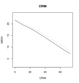
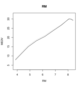
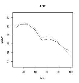
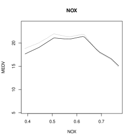
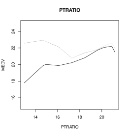
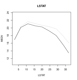
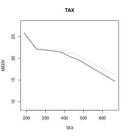
Figure 5: The estimated mean (solid lines) and median (dashed lines) curves of MEDV against each covariate, while other covariates are fixed at their mean values for Boston housing data.

Table 5: The mean squared prediction error (MSPE) from six different methods using quadratic loss for the Boston housing data.

	SDRN	LM	FNN	GBM	RF	GAM
MSE	7.316	15.815	7.655	7.351	7.617	9.297

7.2 Abalone data

The abalone dataset is available at the UCI Machine Learning Repository (Dua and Graff, 2019), which contains 4177 observations and 9 attributes. The attributes are: Sex (male, female and infant), Length (longest shell measurement), Diameter (perpendicular to length), Height (with meat in shell), Whole weight (whole abalone), Shucked weight (weight of meat), Viscera weight (gut weight after bleeding), Shell weight (after being dried) and Rings (+1.5 gives the age in years). The goal is to predict the age of abalone based on these physical measurements. Since the age depends on the Rings, we take the Rings as the response variable. Since Length and Diameter are highly correlated with the correlation coefficient 0.9868 and infant has no gender, we delete Length and Sex and use the remaining six covariates, Diameter, Height, Whole weight, Shucked weight, Viscera weight and Shell weight, in our analysis. In the dataset, there are two observations with zero value for Height, and two other observations are outliers, so we delete these four observations and use the remaining 4173 observations in our analysis.

For exploratory analysis, Figure 6 depicts the scatter plots of the response variable Rings versus Diameter, Height, Whole weight and Shell weight, and the fitted mean curves using cubic B-splines. Clearly, the response has an increasing pattern with these covariates. It has a stronger nonlinear relationship with Whole weight and Shell weight. Table 6 presents the MSPE values in the test data for six different methods using the quadratic loss. We observe that SDRN has a slightly smaller MSPE value than other methods. The coefficient of determination $R^{2}$ obtained from SDRN is 0.587. It is larger than the $R^{2}$ from LM, which is 0.533, due to a clear nonlinear pattern between the response and some of the covariates. Additionally, Figure 7 depicts the fitted mean curves (solid lines) and median curves (dashed lines) of the response Rings versus each of the four covariates obtained from our SDRN method with the quadratic loss and quantile $(\tau=0.5)$ loss, respectively, while other covariates are fixed at their mean values. We see an overall increasing trend of the fitted lines for the four covariates. For Diameter, Whole.weight and Shell.weight, the fitted value of Rings increases steadily as the covariate value increases. However, after the covariate value is beyond a certain point, the estimated value of Rings becomes stable. For Height, the estimated value of Rings increases with Height in the beginning stage, it becomes stable when Height is from 0.7-0.13, and then it increases again. Moreover, the estimated conditional mean function is similar to the estimated conditional median function in general for this dataset.

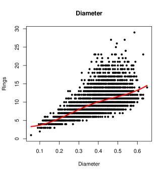
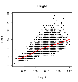
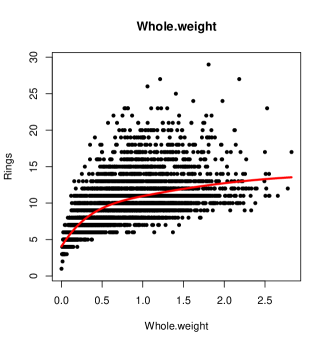
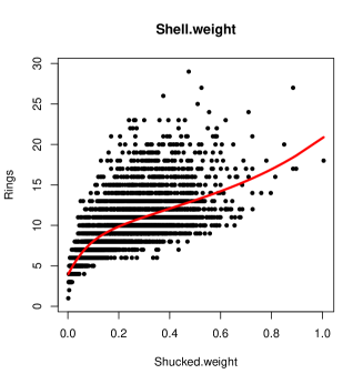
Figure 6: Scatter plots of the response Rings versus four covariates and the fitted mean curve using cubic B-splines.

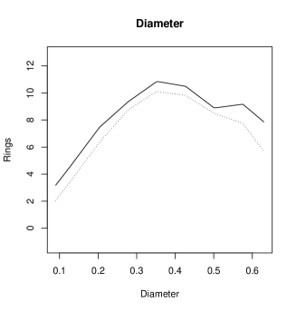
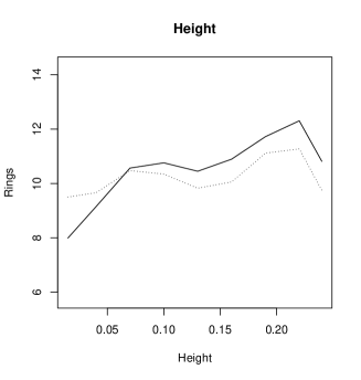
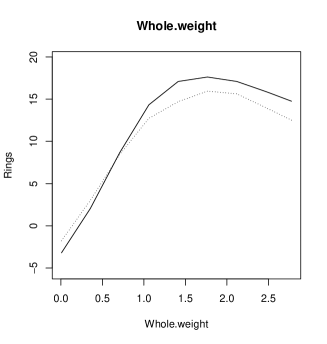
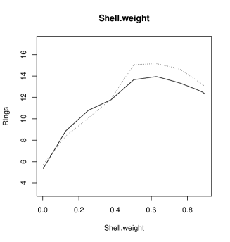
Figure 7: The estimated mean (solid lines) and median (dashed lines) curves of Rings against each covariate, while other covariates are fixed at their mean values for Boston housing data for Abalone data.

Table 6: The mean squared prediction error (MSPE) from the six different methods for the abalone data.

	SDRN	LM	FNN	GBM	RF	GAM
MSE	4.414	4.957	4.482	4.636	4.564	4.560

7.3 Haberman’s Survival Data

The Haberman’s Survival data is available at the UCI Machine Learning Repository (Dua and Graff, 2019). The dataset contains cases from a study conducted at the University of Chicago’s Billings Hospital on the survival of patients who had undergone surgery for breast cancer. It has 306 observations and 4 attributes, which are age of patient at time of operation, patient’s year of operation (minus 1900), the number of positive axillary nodes detected and survival status (survived 5 years or longer or died within 5 years). Based on the survival status column, we define $Y_{i}=1$ if the $i$th patient survived 5 years or longer, otherwise $Y_{i}=0$. Then we apply different machine learning methods to this dataset for classification.

Table 7 presents the accuracy, precision, recall, F1 and AUC (area under the ROC curve) obtained from the test data for the survival group. We observe that SDRN outperforms other methods with the highest accuracy, precision, F1 score and AUC. Figure 8 shows the estimated log-odds functions versus Age and the number of positive axillary nodes, respectively, while other covariates are fixed at their mean values. With age increasing, the estimated log-odds value decreases, indicating decreasing survival probabilities. For the number of positive axillary nodes, the estimated log-odds function drops quickly to a small value when the number of positive axillary nodes increases from 0 to 12, and then it becomes stable and remains at a low point. This result indicates that when the number of positive axillary nodes is within a threshold value, it has a strong adverse effect on the survival probability. However, when it passes the threshold value, the survival probability remains at a very small value. In summary, we can clearly observe a nonlinear pattern of the estimated function in both plots. (Landwehr et al., 1984) also mentioned that the GLM could have a poor performance for this dataset because of the nonlinearity. Moreover, we use McFadden’s pseudo $R^{2}=1-\frac{\text{log}\hat{L}(M_{full})}{\text{log}\hat{L}(M_{null})}$ to further evaluate the model fitting, where $\hat{L}(M_{full})$ is the estimated likelihood with all predictors and $\hat{L}(M_{null})$ is the estimated likelihood without any predictors. The higher value of the pseudo $R^{2}$ indicates better model fitting. The pseudo $R^{2}$ from SDRN is $0.2012$, and it is larger than the pseudo $R^{2}=0.1056$ from GLM.

Table 7: Accuracy, Precision, Recall, F1 and AUC for the survival group obtained by different methods with logistic loss for Haberman’s Survival Data.

	SDRN	GLM	FNN	GBM	RF	GAM
Accuracy	0.714	0.701	0.701	0.688	0.688	0.688
Precision	0.754	0.735	0.750	0.738	0.746	0.738
Recall	0.891	0.909	0.872	0.873	0.845	0.873
F1	0.817	0.813	0.807	0.800	0.797	0.800
AUC	0.677	0.633	0.635	0.641	0.641	0.667

Figure 8: The estimated log-odds functions versus Age and the number of positive axillary nodes, respectively, while other covariates are fixed at their mean values.

7.4 BUPA data

The BUPA Liver Disorders dataset is available at the UCI Machine Learning Repository (Dua and Graff, 2019). It has 345 rows and 7 columns, with each row constituting the record of a single male individual. The first 5 variables are blood tests that are considered to be sensitive to liver disorders due to excessive alcohol consumption; they are mean corpuscular volume (mcv), alkaline phosphotase (alkphos), alanine aminotransferase (sgpt), aspartate aminotransferase (sgot) and gamma-glutamyl transpeptidase (gammagt). We use them as covariates. The 6th variable is the number of half-point equivalents of alcoholic beverages drunk per day. Following McDermott and Forsyth (2016), we dichotomize it to a binary response by letting $Y_{i}=1$ if the number of drinks is greater than 3, otherwise $Y_{i}=0$. The 7th column in the dataset was created by BUOA researchers for traing and test data selection.

We first calculate the McFadden-pseudo $R^{2}$ for GLM and SDRN with logistic loss, respectively. The pseudo $R^{2}$ for GLM is 0.2355, while it is 0.2584 for SDRN, indicating that the SDRN method yields a better prediction. In addition, Table 8 shows the accuracy, precision, recall, F1 and AUC for the group with the number of drinks greater than 3 obtained from the six methods with logistic loss. We see that SDRN has the largest accuracy, recall, F1 and AUC. The accuracy from GLM and GAM is smaller than other methods due to possible model misspecification of these two methods. To explore the nonlinear patterns, Figure 9 depicts the estimated log-odds functions versus the mcv, alkphos, sgot and gammagt predictors, respectively, while other covariates are fixed at their mean values. We can see that the estimated log-odds has a clear increaing pattern with mcv and sgot, indicating that the mcv and sgot levels can be strong indicators for alcohol consumption. For gammagt, the estimated log-odds increases quickly as the the level of gammagt is elevated. Its value remains to be positive as gammagt passes a certain value. The estimated log-odds has a quadratic nonlinear relationship with alkphos. Abnormal (either low or high) levels of alkphos is connected to a few health problems. Low levels of alkphos indicate a deficiency in zinc and magnesium, or a rare genetic disease called hypophosphatasia, which effects bones and teeth. High levels of alkphos can be an indicator of liver disease or bone disorder.

Table 8: Accuracy, Precision Recall, F1 and AUC for the group with the number of drinks greater than 3 of the BUPA data for different methods with logistic loss.

	SDRN	GLM	FNN	GBM	RF	GAM
Accuracy	0.620	0.595	0.615	0.615	0.610	0.605
Precision	0.650	0.634	0.667	0.672	0.653	0.627
Recall	0.520	0.450	0.460	0.450	0.470	0.520
F1	0.578	0.526	0.544	0.539	0.547	0.568
AUC	0.637	0.618	0.629	0.613	0.608	0.624

Figure 9: The estimated log-odds functions versus mcv, alkphos, sgot and gammagt , respectively, while other covariates are fixed at their mean values, for the BUPA data.

8 Discussion

In this paper, we propose a sparse deep ReLU network estimator (SDRN) obtained from empirical risk minimization with a Lipschitz loss function satisfying mild conditions. Our framework can be applied to a variety of regression and classification problems in machine learning. In general, deep neural networks are effective tools for lessening the curse of dimensionality under the condition that the target functions have certain special properties. We assume that the unknown target function belongs to Korobov spaces, which are subsets of the Sobolev spaces commonly used in the nonparametric regression literature. Functions in the Korobov spaces need to have partial mixed derivatives rather than a compositional structure, and thus can be more flexible for investigating nonlinear patterns between the response and the predictors.

We derive non-asymptotic excess risk bounds for SDRN estimator. Our framework allows the dimension of the feature space to increase with the sample size with a rate slightly slower than $\log(n)$. We further show that our SDRN estimator can achieve the same optimal minimax rate (up to logarithmic factors) as one-dimensional nonparametric regression when the dimension is fixed, and the dimensionality effect is passed on to a logarithmic factor, so the curse of dimensionality is alleviated. The SDRN estimator has a suboptimal rate when the dimension increases with the sample size. Moreover, the depth and the total number of nodes and weights of the network need to increase with the sample size with certain rates established in the paper. These statistical properties provide an important theoretical basis and guidance for the analytic procedures in data analysis. Practically, we illustrate the proposed method through simulation studies and several real data applications. The numerical studies support our theoretical results.

Our proposed method provides a reliable solution for mitigating the curse of dimensionality for modern data analysis. Meanwhile it has opened up several interesting new avenues for further work. One extension is to derive a similar estimator for smoother regression functions with mixed derivatives of order greater than two; Jacobi-weighted Korobov spaces (Shen and Wang, 2010) may be considered for this scenario. Our method can be extended to other settings such as semiparametric models, longitudinal data and $L_{1}$ penalized regression. Moreover, it can be a promising tool for estimation of the propensity score function or the outcome regression function used in treatment effect studies. These interesting topics deserve thorough investigations for future research.

Appendix

In the Appendix, we provide additional simulation results, the discussions of sparse grids approximation, the technical proofs and the computational algorithm.

A.1 Additional simulation results

Tables A.9 and A.10 below show the average MSE, average $\text{bias}^{2}$ and average variance for Model 2 given in Section 6.1 when $n=2000,5000$.

Table A.9: The average MSE, $\text{bias}^{2}$ and variance of the SDRN estimators obtained from the quadratic and quantile $\left(\tau=0.5,\ 0.25\right)$ loss functions based on the 100 simulation replications when $n=2000$ for Model 2.

		quadratic					quantile ($\tau=0.5)$					quantile ($\tau=0.25)$
$\kappa$		$c=-2$	$c=-1$	$c=0$	$c=1$	$c=2$	$c=-2$	$c=-1$	$c=0$	$c=1$	$c=2$	$c=-2$	$c=-1$	$c=0$	$c=1$	$c=2$
		Normal	error
$0.1$	bias2	0.2400	0.1005	0.0936	0.0462	0.0392	0.2423	0.1098	0.0971	0.0512	0.0392	0.2500	0.1163	0.1058	0.1105	0.1629
	var	0.0414	0.1149	0.2878	0.5325	0.6728	0.0357	0.0949	0.2274	0.4545	0.6739	0.0358	0.0943	0.2189	0.4127	0.6366
	mse	0.2814	0.2154	0.3814	0.5787	0.7119	0.2780	0.2047	0.3246	0.5058	0.7131	0.2858	0.2106	0.3247	0.5232	0.7995
$0.5$	bias2	0.2417	0.1222	0.1033	0.0644	0.0476	0.2568	0.1532	0.1189	0.0791	0.0538	0.2625	0.1649	0.1216	0.0870	0.0918
	var	0.0184	0.0479	0.1096	0.2110	0.3344	0.0120	0.0349	0.0794	0.1617	0.3090	0.0111	0.0334	0.0757	0.1534	0.3129
	mse	0.2601	0.1701	0.2129	0.2754	0.3820	0.2688	0.1881	0.1983	0.2408	0.3628	0.2737	0.1983	0.1973	0.2404	0.4048
$1$	bias2	0.2470	0.1426	0.1138	0.0772	0.0563	0.2877	0.1822	0.1407	0.0990	0.0690	0.2814	0.1934	0.1438	0.1003	0.0802
	var	0.0113	0.0310	0.0697	0.1363	0.2282	0.0063	0.0210	0.0482	0.0985	0.1842	0.0056	0.0196	0.0453	0.0925	0.2465
	mse	0.2583	0.1735	0.1834	0.2135	0.2845	0.2940	0.2031	0.1888	0.1975	0.2532	0.2871	0.2130	0.1892	0.1928	0.3267
$2$	bias2	0.2639	0.1687	0.1315	0.0941	0.0695	0.3649	0.2154	0.1720	0.1271	0.0922	0.3156	0.2226	0.1731	0.1260	0.0926
	var	0.0063	0.0192	0.0432	0.0855	0.1487	0.0030	0.0118	0.0282	0.0580	0.1100	0.0025	0.0108	0.0260	0.0562	0.1547
	mse	0.2702	0.1879	0.1747	0.1796	0.2182	0.3679	0.2272	0.2002	0.1850	0.2023	0.3181	0.2334	0.1991	0.1822	0.2473
$4$	bias2	0.3108	0.1982	0.1582	0.1177	0.0884	0.5242	0.2598	0.2112	0.1657	0.1246	0.3629	0.2551	0.2051	0.1583	0.1209
	var	0.0032	0.0113	0.0260	0.0518	0.0926	0.0013	0.0062	0.0157	0.0329	0.0696	0.0009	0.0054	0.0141	0.0339	0.1028
	mse	0.3140	0.2095	0.1842	0.1696	0.1810	0.5255	0.2660	0.2269	0.1986	0.1942	0.3639	0.2606	0.2193	0.1922	0.2237
		Laplace	error
$0.1$	bias2	0.2410	0.1021	0.0946	0.0521	0.0448	0.2431	0.1104	0.0966	0.0535	0.0449	0.2559	0.1258	0.1019	0.0822	0.1605
	var	0.0774	0.2202	0.5546	1.0523	1.3398	0.0382	0.1015	0.2661	0.5975	1.0618	0.0466	0.1294	0.3051	0.6110	0.9585
	mse	0.3184	0.3224	0.6492	1.1044	1.3846	0.2813	0.2118	0.3627	0.6510	1.1067	0.3025	0.2552	0.4070	0.6932	1.1189
$0.5$	bias2	0.2416	0.1231	0.1033	0.0661	0.0501	0.2595	0.1557	0.1196	0.0803	0.0580	0.2693	0.1785	0.1307	0.0869	0.0661
	var	0.0350	0.0917	0.2105	0.4144	0.6626	0.0124	0.0362	0.0847	0.1821	0.3908	0.0139	0.0440	0.1018	0.2093	0.4346
	mse	0.2766	0.2148	0.3139	0.4805	0.7127	0.2719	0.1919	0.2043	0.2624	0.4488	0.2832	0.2224	0.2325	0.2962	0.5006
$1$	bias2	0.2461	0.1431	0.1137	0.0779	0.0578	0.2915	0.1855	0.1424	0.1002	0.0719	0.2912	0.2061	0.1562	0.1075	0.0775
	var	0.0217	0.0592	0.1336	0.2664	0.4505	0.0065	0.0218	0.0506	0.1063	0.2153	0.0069	0.0253	0.0601	0.1257	0.3346
	mse	0.2678	0.2023	0.2473	0.3443	0.5083	0.2980	0.2073	0.1930	0.2066	0.2872	0.2982	0.2314	0.2162	0.2332	0.4121
$2$	bias2	0.2619	0.1688	0.1315	0.0943	0.0702	0.3702	0.2192	0.1750	0.1291	0.0938	0.3284	0.2345	0.1863	0.1380	0.0985
	var	0.0122	0.0366	0.0825	0.1660	0.2923	0.0031	0.0123	0.0295	0.0612	0.1209	0.0031	0.0135	0.0338	0.0749	0.1876
	mse	0.2742	0.2054	0.2139	0.2603	0.3625	0.3733	0.2316	0.2046	0.1903	0.2147	0.3314	0.2481	0.2202	0.2130	0.2861
$4$	bias2	0.3076	0.1976	0.1580	0.1177	0.0886	0.5337	0.2647	0.2149	0.1693	0.1273	0.3748	0.2680	0.2178	0.1752	0.1332
	var	0.0063	0.0216	0.0494	0.0998	0.1808	0.0013	0.0064	0.0165	0.0344	0.0712	0.0012	0.0067	0.0180	0.0436	0.0918
	mse	0.3139	0.2191	0.2074	0.2175	0.2694	0.5351	0.2711	0.2315	0.2036	0.1985	0.3759	0.2747	0.2358	0.2188	0.2250

Table A.10: The average MSE, $\text{bias}^{2}$ and variance of the SDRN estimators obtained from the quadratic and quantile $\left(\tau=0.5,\ 0.25\right)$ loss functions based on the 100 simulation replications when $n=5000$ for Model 2.

		quadratic					quantile ($\tau=0.5)$					quantile ($\tau=0.25)$
$\kappa$		$c=-2$	$c=-1$	$c=0$	$c=1$	$c=2$	$c=-2$	$c=-1$	$c=0$	$c=1$	$c=2$	$c=-2$	$c=-1$	$c=0$	$c=1$	$c=2$
		Normal	error
$0.1$	bias2	0.2328	0.0938	0.0851	0.0282	0.0210	0.2343	0.0970	0.0863	0.0316	0.0211	0.2432	0.1011	0.0900	0.0628	0.1419
	var	0.0226	0.0677	0.1927	0.4270	0.7133	0.0235	0.0636	0.1660	0.3637	0.6593	0.0244	0.0652	0.1670	0.3485	0.5866
	mse	0.2554	0.1614	0.2777	0.4552	0.7343	0.2578	0.1605	0.2524	0.3952	0.6804	0.2676	0.1663	0.2570	0.4114	0.7285
$0.5$	bias2	0.2335	0.1020	0.0886	0.0389	0.0240	0.2389	0.1198	0.0961	0.0517	0.0289	0.2476	0.1293	0.0989	0.0591	0.0645
	var	0.0130	0.0330	0.0816	0.1686	0.3035	0.0104	0.0273	0.0638	0.1341	0.2846	0.0104	0.0272	0.0631	0.1323	0.3053
	mse	0.2465	0.1350	0.1702	0.2075	0.3275	0.2493	0.1471	0.1599	0.1858	0.3135	0.2579	0.1565	0.1620	0.1914	0.3698
$1$	bias2	0.2350	0.1130	0.0933	0.0489	0.0292	0.2476	0.1412	0.1070	0.0664	0.0396	0.2547	0.1528	0.1108	0.0700	0.0478
	var	0.0090	0.0226	0.0537	0.1102	0.2014	0.0063	0.0177	0.0403	0.0840	0.1811	0.0061	0.0173	0.0394	0.0824	0.2271
	mse	0.2440	0.1357	0.1470	0.1591	0.2305	0.2538	0.1589	0.1473	0.1504	0.2207	0.2608	0.1701	0.1503	0.1524	0.2749
$2$	bias2	0.2395	0.1310	0.1018	0.0620	0.0380	0.2709	0.1686	0.1259	0.0849	0.0546	0.2705	0.1806	0.1310	0.0872	0.0577
	var	0.0057	0.0149	0.0343	0.0703	0.1300	0.0034	0.0109	0.0248	0.0510	0.0982	0.0031	0.0104	0.0239	0.0506	0.1100
	mse	0.2451	0.1459	0.1362	0.1323	0.1679	0.2743	0.1795	0.1507	0.1360	0.1528	0.2736	0.1910	0.1549	0.1378	0.1677
$4$	bias2	0.2524	0.1554	0.1168	0.0782	0.0512	0.3296	0.2001	0.1547	0.1102	0.0763	0.3004	0.2095	0.1589	0.1117	0.0770
	var	0.0032	0.0094	0.0214	0.0437	0.0813	0.0017	0.0063	0.0148	0.0302	0.0575	0.0014	0.0058	0.0139	0.0301	0.0719
	mse	0.2556	0.1648	0.1382	0.1219	0.1325	0.3313	0.2064	0.1695	0.1404	0.1337	0.3018	0.2153	0.1728	0.1418	0.1489
		Laplace	error
$0.1$	bias2	0.2329	0.0937	0.0862	0.0326	0.0281	0.2356	0.0963	0.0860	0.0334	0.0248	0.2495	0.1072	0.0920	0.0467	0.0884
	var	0.0407	0.1280	0.3696	0.8463	1.4189	0.0244	0.0647	0.1831	0.4419	0.9316	0.0301	0.0883	0.2283	0.4951	0.8929
	mse	0.2736	0.2218	0.4558	0.8790	1.4470	0.2600	0.1610	0.2691	0.4753	0.9564	0.2796	0.1955	0.3203	0.5417	0.9813
$0.5$	bias2	0.2336	0.1019	0.0890	0.0405	0.0270	0.2413	0.1195	0.0956	0.0522	0.0308	0.2545	0.1409	0.1057	0.0613	0.0432
	var	0.0233	0.0620	0.1562	0.3317	0.5988	0.0105	0.0266	0.0650	0.1426	0.3189	0.0121	0.0350	0.0824	0.1769	0.3833
	mse	0.2569	0.1638	0.2452	0.3722	0.6257	0.2519	0.1461	0.1605	0.1948	0.3498	0.2666	0.1759	0.1881	0.2382	0.4264
$1$	bias2	0.2352	0.1129	0.0935	0.0499	0.0311	0.2513	0.1417	0.1064	0.0664	0.0408	0.2633	0.1663	0.1203	0.0765	0.0488
	var	0.0162	0.0422	0.1024	0.2157	0.3966	0.0063	0.0171	0.0402	0.0858	0.2053	0.0070	0.0218	0.0509	0.1080	0.2877
	mse	0.2514	0.1551	0.1959	0.2656	0.4277	0.2576	0.1588	0.1466	0.1522	0.2461	0.2703	0.1881	0.1711	0.1845	0.3365
$2$	bias2	0.2398	0.1310	0.1019	0.0626	0.0392	0.2766	0.1704	0.1257	0.0846	0.0552	0.2823	0.1945	0.1434	0.0972	0.0636
	var	0.0103	0.0277	0.0651	0.1367	0.2551	0.0034	0.0106	0.0243	0.0509	0.1027	0.0036	0.0128	0.0304	0.0642	0.1811
	mse	0.2501	0.1586	0.1669	0.1993	0.2943	0.2800	0.1810	0.1500	0.1354	0.1579	0.2859	0.2073	0.1738	0.1613	0.2447
$4$	bias2	0.2530	0.1556	0.1168	0.0786	0.0519	0.3377	0.2036	0.1554	0.1098	0.0763	0.3157	0.2235	0.1731	0.1251	0.0866
	var	0.0059	0.0173	0.0401	0.0841	0.1588	0.0017	0.0062	0.0144	0.0297	0.0586	0.0017	0.0070	0.0174	0.0386	0.0943
	mse	0.2589	0.1729	0.1569	0.1626	0.2108	0.3394	0.2099	0.1698	0.1395	0.1349	0.3174	0.2306	0.1905	0.1637	0.1809

A.2 Sparse grids approximation

In this section, we introduce a hierarchical basis of piecewise linear functions. We have discussed a connection between this hierarchical basis and a ReLU network in Section 3. For any functions in the Korobov spaces satisfying Assumption 1, they have a unique representation in this hierarchical basis. To approximate functions of one variable $x$ on $[0,1]$, a simple choice of a basis function is the standard hat function $\phi(x)$:

$$\phi(x)=\left\{\begin{array}[]{cc}1-|x|,&\text{if }x\in[-1,1]\\ 0,&\text{otherwise.}\end{array}\right.$$

To generate a one-dimensional hierarchical basis, we consider a family of grids $\Omega_{\ell}$ of level $\ell$ characterized by a grid size $h_{\ell}=2^{-\ell}$ and $2^{\ell}+1$ points $x_{\ell,s}=sh_{\ell}$ for $0\leq s\leq 2^{\ell}$. On each $\Omega_{\ell}$, the piecewise linear basis functions $\phi_{\ell,s}$ are given as

$$\phi_{\ell,s}(x)=\phi(\frac{x-x_{\ell,s}}{h_{\ell}})\text{, }0\leq s\leq 2^{\ell},$$

on the support $\left[x_{\ell,s}-h_{\ell},x_{\ell,s}+h_{\ell}\right]\cap\left[0,1\right]$. Note that $||\phi_{\ell,s}||_{\infty}\leq 1$ for all $\ell$ and $s$. The hierarchical increment spaces $W_{\ell}$ on each $\Omega_{\ell}$ are given by

$$W_{\ell}=\text{span}\{\phi_{\ell,s}:s\in I_{\ell}\},$$

where $I_{\ell}=\{s\in\mathbb{N}:0\leq s\leq 2^{\ell}$; $s$ are odd numbers for $\ell\geq 1\}$. We can see that for each $\ell\geq 1$, the supports of all basis functions $\phi_{\ell,s}$ spanning $W_{\ell}$ are mutually disjoint. Then the hierarchical space of functions up to level $L$ is

$$V_{L}=\bigoplus\limits_{0\leq\ell\leq L}W_{\ell}=\text{span}\{\phi_{\ell,s}:s\in I_{\ell},0\leq\ell\leq L\}.$$

To approximate functions of $d$-dimensional variables $\boldsymbol{x=}\mathbf{(}x_{1},\ldots,x_{d})^{\top}$ on $\mathcal{X}=[0,1]^{d}$,  we employ a tensor product construction of the basis functions. We consider a family of grids $\Omega_{\boldsymbol{\ell}}$ of level $\boldsymbol{\ell}=(\ell_{1},...,\ell_{d})^{\top}$ with interior points $\boldsymbol{x}_{\boldsymbol{\ell},\boldsymbol{s}}=\boldsymbol{s}\cdot\boldsymbol{h}_{\boldsymbol{\ell}}$, where $\boldsymbol{h}_{\boldsymbol{\ell}}=(h_{\ell_{1}},...,h_{\ell_{d}})^{\top}$ with $h_{\ell_{j}}=2^{-\ell_{j}}$ and $\boldsymbol{s}=(s_{1},...,s_{d})^{\top}$ for $0\leq s_{j}\leq 2^{\ell_{j}}$ and $j=1,...,d$. On each $\Omega_{\boldsymbol{\ell}}$, the basis functions $\phi_{\boldsymbol{\ell},\boldsymbol{s}}$ are given as

$$\phi_{\boldsymbol{\ell},\boldsymbol{s}}(\boldsymbol{x})=\prod\limits_{j=1}^{d}\phi_{\ell_{j},s_{j}}(x_{j})\text{, }\boldsymbol{0}_{d}\leq\boldsymbol{s}\leq 2^{\boldsymbol{\ell}},$$

and they satisfy $||\phi_{\boldsymbol{\ell},\boldsymbol{s}}||_{\infty}\leq 1$. The hierarchical increment spaces $W_{\boldsymbol{\ell}}$ are given by

$$W_{\boldsymbol{\ell}}=\text{span}\{\phi_{\boldsymbol{\ell},\boldsymbol{s}}(\boldsymbol{x}):\boldsymbol{s}\in I_{\boldsymbol{\ell}}\},$$

where $I_{\boldsymbol{\ell}}=I_{\ell_{1}}\times\cdots\times I_{\ell_{d}}$, and $I_{\ell j}=\{s_{j}\in\mathbb{N}:0\leq s_{j}\leq 2^{\ell_{j}},s_{j}$ are odd numbers for $\ell_{j}\geq 1\}$. Then the hierarchical space of functions up to level $\boldsymbol{L}=(L_{1},...,L_{d})^{\top}$ is

$$V_{\boldsymbol{L}}=\bigoplus\limits_{\boldsymbol{0}\leq\boldsymbol{\ell}\leq\boldsymbol{L}}W_{\boldsymbol{\ell}}=\text{span}\{\phi_{\boldsymbol{\ell},\boldsymbol{s}}:\boldsymbol{s}\in I_{\boldsymbol{\ell}},\boldsymbol{0}_{d}\leq\boldsymbol{\ell}\leq\boldsymbol{L}\}.$$

For any function $f\in W^{2,p}(\mathcal{X)}$, it has a unique expression in the hierarchical basis (Bungartz and Griebel (2004)):

$$f(\boldsymbol{x})=\sum_{\boldsymbol{0}_{d}\leq\boldsymbol{\ell}\leq\boldsymbol{\infty}}\sum_{s\in I_{\boldsymbol{\ell}}}\gamma_{{}_{\boldsymbol{\ell},\boldsymbol{s}}}^{0}\phi_{\boldsymbol{\ell},\boldsymbol{s}}(\boldsymbol{x})=\sum_{\boldsymbol{0}_{d}\leq\boldsymbol{\ell}\leq\boldsymbol{\infty}}g_{\boldsymbol{\ell}}(\boldsymbol{x}),$$ (A.1)

where $g_{\boldsymbol{\ell}}(\boldsymbol{x})=\sum_{s\in I_{\boldsymbol{\ell}}}\gamma_{{}_{\boldsymbol{\ell},\boldsymbol{s}}}^{0}\phi_{\boldsymbol{\ell},\boldsymbol{s}}(\boldsymbol{x})\in W_{\boldsymbol{\ell}}$. The hierarchical coefficients $\gamma_{{}_{\boldsymbol{\ell},\boldsymbol{s}}}^{0}\in\mathbb{R}$ are given as (Lemma 3.2 of Bungartz and Griebel (2004)):

$$\gamma_{{}_{\boldsymbol{\ell},\boldsymbol{s}}}^{0}=\int_{\mathcal{X}}\prod\limits_{j=1}^{d}\left(-2^{-(\boldsymbol{\ell}_{j}+1)}\phi_{\ell_{j},s_{j}}(x_{j})\right)D^{\boldsymbol{2}}f(\boldsymbol{x})d\boldsymbol{x}$$ (A.2)

where $\boldsymbol{2}=2\boldsymbol{1}_{d}$, and satisfy (Lemma 3.3 of Bungartz and Griebel (2004))

$$|\gamma_{{}_{\boldsymbol{\ell},\boldsymbol{s}}}^{0}|\leq 6^{-d/2}2^{-(3/2)|\boldsymbol{\ell}|_{1}}(\int\nolimits_{\boldsymbol{x}_{\boldsymbol{\ell},\boldsymbol{s}}-\boldsymbol{h}_{\boldsymbol{\ell}}}^{\boldsymbol{x}_{\boldsymbol{\ell},\boldsymbol{s}}+\boldsymbol{h}_{\boldsymbol{\ell}}}|D^{\boldsymbol{2}}f(\boldsymbol{x})|^{2}d\boldsymbol{x})^{1/2}\leq 6^{-d/2}2^{-(3/2)|\boldsymbol{\ell}|_{1}}||D^{\boldsymbol{2}}f||_{L^{2}}.$$ (A.3)

Moreover, the above result leads to (Lemma 3.4 of Bungartz and Griebel (2004))

$$||g_{\boldsymbol{\ell}}||_{L^{2}}\leq 3^{-d}2^{-2|\boldsymbol{\ell}|_{1}}(\int\nolimits_{\mathcal{X}}|D^{\boldsymbol{2}}f(\boldsymbol{x})|^{2}d\boldsymbol{x})^{1/2}=3^{-d}2^{-2|\boldsymbol{\ell}|_{1}}||D^{\boldsymbol{2}}f||_{L^{2}}.$$ (A.4)

Assumption 3 and (A.4) imply that

$$||g_{\boldsymbol{\ell}}||_{2}\leq c_{\mu}||g_{\boldsymbol{\ell}}||_{L^{2}}\leq c_{\mu}3^{-d}2^{-2|\boldsymbol{\ell}|_{1}}||D^{\boldsymbol{2}}f||_{L^{2}}.$$ (A.5)

In practice, one can use a truncated version to approximate the function $f(\cdot)$ given in (A.1), so that

$$f(\boldsymbol{x})\approx\sum\nolimits_{0\leq|\boldsymbol{\ell|}_{\infty}\leq m}\sum\nolimits_{s\in I_{\boldsymbol{\ell}}}\gamma_{{}_{\boldsymbol{\ell},\boldsymbol{s}}}^{0}\phi_{\boldsymbol{\ell},\boldsymbol{s}}(\boldsymbol{x})=\sum\nolimits_{0\leq|\boldsymbol{\ell|}_{\infty}\leq m}g_{\boldsymbol{\ell}}(\boldsymbol{x}),$$

which is constructed based on the space with full grids: $V_{m}^{\left(\infty\right)}=\bigoplus\limits_{0\leq|\boldsymbol{\ell|}_{\infty}\leq m}W_{\boldsymbol{\ell}}=$span$\{\phi_{\boldsymbol{\ell},\boldsymbol{s}}:s\in I_{\boldsymbol{\ell}},0\leq|\boldsymbol{\ell}|_{\infty}\leq m\}$. The dimension of the space $V_{m}^{\left(\infty\right)}$ is $|V_{m}^{\left(\infty\right)}|=(2^{m}+1)^{d}$, which increases with $d$ in an exponential order. For dimension reduction, we consider the hierarchical space with sparse grids:

$$V_{m}^{\left(1\right)}=\bigoplus\limits_{|\boldsymbol{\ell|}_{1}\leq m}W_{\boldsymbol{\ell}}=\text{span}\{\phi_{\boldsymbol{\ell},\boldsymbol{s}}:s\in I_{\boldsymbol{\ell}},|\boldsymbol{\ell}|_{1}\leq m\}.$$

The function $f(\cdot)$ given in (A.1) can be approximated by

$$f_{m}(\boldsymbol{x})=\sum\nolimits_{|\boldsymbol{\ell|}_{1}\leq m}\sum\nolimits_{s\in I_{\boldsymbol{\ell}}}\gamma_{{}_{\boldsymbol{\ell},\boldsymbol{s}}}^{0}\phi_{\boldsymbol{\ell},\boldsymbol{s}}(\boldsymbol{x})=\sum\nolimits_{|\boldsymbol{\ell|}_{1}\leq m}g_{\boldsymbol{\ell}}(\boldsymbol{x}).$$ (A.6)

Clearly, when $d=1$, the dimension of the hierarchical space with sparse grids is the same as that of the space with full grids. The dimensionality issue does not exist. For the rest of this paper, we assume that $d\geq 2$. Table A.11 provides the number of basis functions for the hierarchical space with sparse grids $V_{m}^{\left(1\right)}$ and the space with full grids $V_{m}^{\left(\infty\right)}$ when the dimension of the covariates $d$ increases from 2 to 8 and the $m$ value increases from 0 to 4. We see that the number of basis functions for the space with sparse grids is dramatically reduced compared to the space with full grids, when the dimension $d$ or $m$ value become larger, so that the dimensionality problem can be lessened.

Table A.11: The number of basis functions for the space with sparse grids and the space with full grids.

	Sparse grids					Full grids
	$m=0$	$m=1$	$m=2$	$m=3$	$m=4$	$m=0$	$m=1$	$m=2$	$m=3$	$m=4$
$d=2$	$4$	$8$	$17$	$37$	$81$	$4$	$9$	$25$	$81$	$289$
$d=3$	$8$	$20$	$50$	$123$	$297$	$8$	$27$	$125$	$729$	$4913$
$d=4$	$16$	$48$	$136$	$368$	$961$	$16$	$81$	$625$	$6561$	$83521$
$d=5$	$32$	$112$	$352$	$1032$	$2882$	$32$	$243$	$3125$	$59049$	$1419857$
$d=6$	$64$	$256$	$880$	$2768$	$8204$	$64$	$729$	$15625$	$531441$	$24137569$
$d=7$	$128$	$576$	$2144$	$7184$	$22472$	$128$	$2187$	$78125$	$4782969$	$410338673$
$d=8$	$256$	$1280$	$5120$	$18176$	$59744$	$256$	$6561$	$390625$	$43046721$	$6975757441$

The following proposition provides the approximation error of the approximator $f_{m}\left(\cdot\right)$ obtained from the sparse grids to the true unknown function $f\in W^{2,p}(\mathcal{X)}$.

Proposition A.1.

For any $f\in W^{2,p}(\mathcal{X)}$, $2\leq p\leq\infty$, under Assumption 3, one has that for $d=2$, $||f_{m}-f||_{2}\leq 18^{-1}c_{\mu}2^{-2m}(m+3)||D^{\boldsymbol{2}}f||_{L^{2}}$; for $d\geq 3$,

$$||f_{m}-f||_{2}\leq\widetilde{c}2^{-2m}\sqrt{d-2}\left(\frac{e}{3}\frac{m+d}{d-2}\right)^{d-1}||D^{\boldsymbol{2}}f||_{L^{2}},$$ (A.7)

where $\widetilde{c}=2^{-1}c_{\mu}(3\sqrt{2\pi}e)^{-1}$.

Proposition A.1 shows that the approximator error decreases as the $m$ value increases.

A.3 Proof of Proposition 1

In this section, we provide the proof of Proposition 1. The dimension of $W_{\boldsymbol{\ell}}$ satisfies

$$|W_{\boldsymbol{\ell}}|\leq\prod\nolimits_{j=1}^{d}2^{\ell_{j}\vee 2-1}=2^{\sum_{j=1}^{d}\ell_{j}\vee 2-d}.$$

Thus,

$$|V_{m}^{\left(1\right)}| \leq \sum\nolimits_{|\boldsymbol{\ell|}_{1}\leq m}2^{\sum_{j=1}^{d}\ell_{j}\vee 2-d}\leq\sum\nolimits_{|\boldsymbol{\ell|}_{1}\leq m}2^{|\boldsymbol{\ell|}_{1}+d}=\sum_{k=0}^{m}2^{k+d}\binom{d-1+k}{d-1}$$

$$= 2^{d}\sum_{k=0}^{m}2^{k}\binom{d-1+k}{d-1}=2^{d}\left\{(-1)^{d}+2^{m+1}\sum_{k=0}^{d-1}\binom{m+d}{k}(-2)^{d-1-k}\right\},$$

where the last equality follows from (3.62) of Bungartz and Griebel (2004). We assume that $d$ is even. The result for odd $d$ can be proved similarly. Then

$$\sum_{k=0}^{d-1}\binom{m+d}{k}(-2)^{d-1-k}=\sum_{v=0}^{d/2-1}2^{2v}\left\{\binom{m+d}{d-(1+2v)}-2\binom{m+d}{d-(2+2v)}\right\}.$$

Moreover,

$$\binom{m+d}{d-(1+2v)}-2\binom{m+d}{d-(2+2v)}$$

$$= \frac{(m+d)!}{(d-(1+2v))!(m+1+2v)!}-2\frac{(m+d)!}{(d-(2+2v))!(m+2v+2)!}$$

$$= \frac{(m+d)!}{(d-(2+2v))!(m+1+2v)!}\left\{\frac{1}{d-(1+2v)}-\frac{2}{m+2v+2}\right\}$$

$$= \frac{(m+d)!(m+6v-2d+4)}{(d-(1+2v))!(m+2v+2)!}$$

$$= \frac{(m+d)(m+d-1)\times\cdot\cdot\cdot\times(m+2v+3)(m+6v-2d+4)}{(d-(1+2v))!}$$

$$\leq \frac{(m+d)^{(d-(2+2v))}}{(d-(1+2v))!}.$$

Thus,

$$\sum_{k=0}^{d-1}\binom{m+d}{k}(-2)^{d-1-k}\leq\sum_{v=0}^{d/2-1}2^{2v}\frac{(m+d)^{(d-(2+2v))}}{(d-(1+2v))!}\leq 2^{d-2}\frac{(m+d)^{(d-2)}}{(d-1)!}.$$

By stirling’s formula,

$$(d-1)!\geq\sqrt{2\pi}(d-1)^{d-1/2}e^{-(d-1)}.$$

Therefore,

$$\sum_{k=0}^{d-1}\binom{m+d}{k}(-2)^{d-1-k}\leq 2^{d-2}\frac{(m+d)^{(d-2)}}{\sqrt{2\pi}(d-1)^{d-1/2}e^{-(d-1)}},$$

and hence

$$|V_{m}^{\left(1\right)}|\leq 2^{d+1}2^{m+1}2^{d-2}\frac{(m+d)^{(d-2)}e^{(d-1)}}{\sqrt{2\pi}(d-1)^{d-1/2}}=2\sqrt{\frac{2}{\pi}}\frac{\sqrt{d-1}}{\left(m+d\right)}2^{m}\left(4e\frac{m+d}{d-1}\right)^{d-1}.$$

Moreover, let $\boldsymbol{\ell}_{-1}=(\ell_{2},\ldots,\ell_{d})^{\top}$. Then, $|V_{0}^{\left(1\right)}|=\sum\nolimits_{|\boldsymbol{\ell|}_{1}=0}\prod\nolimits_{j=1}^{d}2=2^{d}$, and for $m\geq 1$,

$$|V_{m}^{\left(1\right)}| \geq \sum\nolimits_{|\boldsymbol{\ell|}_{1}=0}\prod\nolimits_{j=1}^{d}2+\sum\nolimits_{1\leq\ell_{1}\leq m,|\boldsymbol{\ell}_{-1}\boldsymbol{|}_{1}=0}(\prod\nolimits_{j=2}^{d}2)2^{\ell_{1}-1}=2^{d}+2^{d-1}\sum\nolimits_{1\leq\ell_{1}\leq m}2^{\ell_{1}-1}$$

$$= 2^{d}+2^{d-1}(2^{m}-1)=2^{d-1}(2^{m}-1+2)\geq 2^{d-1}(2^{m}+1).$$

Therefore, $|V_{m}^{\left(1\right)}|\geq 2^{d-1}(2^{m}+1)$ for any $m\geq 0$.

A.4 Proof of Proposition A.1

This section provides the proof of Proposition A.1. Based on (A.1) and (A.6), one has

$$||f_{m}-f||_{2}=||\sum_{\boldsymbol{1}_{d}\leq\boldsymbol{\ell}\leq\boldsymbol{\infty}}g_{\boldsymbol{\ell}}(\boldsymbol{x})-\sum_{|\boldsymbol{\ell|}_{1}\leq m}g_{\boldsymbol{\ell}}(\boldsymbol{x})||_{2}=||\sum_{|\boldsymbol{\ell|}_{1}>m}g_{\boldsymbol{\ell}}(\boldsymbol{x})||_{2}.$$

By (A.5) and Assumption 3, one has

$$||\sum_{|\boldsymbol{\ell|}_{1}>m}g_{\boldsymbol{\ell}}(\boldsymbol{x})||_{2} \leq \sum_{|\boldsymbol{\ell|}_{1}>m}||g_{\boldsymbol{\ell}}||_{2}\leq\sum_{|\boldsymbol{\ell|}_{1}>m}c_{\mu}3^{-d}2^{-2|\boldsymbol{\ell}|_{1}}||D^{\boldsymbol{2}}f||_{L^{2}}$$

$$= c_{\mu}3^{-d}||D^{\boldsymbol{2}}f||_{L^{2}}\sum_{|\boldsymbol{\ell|}_{1}>m}2^{-2|\boldsymbol{\ell}|_{1}}.$$

Then, one has that for arbitrary $s\in\mathbb{N}$,

$$\sum_{|\boldsymbol{\ell|}_{1}>m}2^{-s|\boldsymbol{\ell}|_{1}} = \sum_{k^{\prime}=m+1}^{\infty}2^{-sk^{\prime}}\binom{k^{\prime}+d-1}{d-1}=\sum_{k=0}^{\infty}2^{-s\left(k+m+1\right)}\binom{k+m+1+d-1}{d-1}$$

$$= 2^{-s\left(m+1\right)}\sum_{k=0}^{\infty}2^{-sk}\binom{k+m+1+d-1}{d-1}$$

$$\leq 2^{-s\left(m+1\right)}2A(d,m),$$

where $A(d,m)=\sum\nolimits_{k=0}^{d-1}\binom{m+d}{k}$, where the last inequality follows from Lemma 3.7 of Bungartz and Griebel (2004).

$$||f_{m}-f||_{2} \leq \sum_{|\boldsymbol{\ell|}_{1}>m}||g_{\boldsymbol{\ell}}||_{2}\leq c_{\mu}3^{-d}||D^{\boldsymbol{2}}f||_{L^{2}}2^{-2\left(m+1\right)}2A(d,m)$$

$$= 2^{-1}c_{\mu}2^{-2m}3^{-d}A(d,m)||D^{\boldsymbol{2}}f||_{L^{2}}.$$

Moreover, for $d\geq 3$, $A(d,m)\leq(d-1)\frac{(m+d)^{d-1}}{(d-1)!}=\frac{(m+d)^{d-1}}{(d-2)!}$, and by stirling’s formula,

$$(d-2)!\geq\sqrt{2\pi}(d-2)^{d-3/2}e^{-(d-2)}.$$

Then

$$A(d,m)\leq\frac{(m+d)^{d-1}}{\sqrt{2\pi}(d-2)^{d-3/2}e^{-(d-2)}}=\frac{\sqrt{d-2}}{\sqrt{2\pi}}\left(\frac{m+d}{d-2}\right)^{d-1}e^{(d-2)}.$$

Therefore,

$$||f_{m}-f||_{2} \leq 2^{-1}c_{\mu}2^{-2m}3^{-d}\frac{\sqrt{d-2}}{\sqrt{2\pi}}\left(\frac{m+d}{d-2}\right)^{d-1}e^{(d-2)}||D^{\boldsymbol{2}}f||_{L^{2}}$$

$$= \widetilde{c}2^{-2m}\sqrt{d-2}\left(\frac{e}{3}\frac{m+d}{d-2}\right)^{d-1}||D^{\boldsymbol{2}}f||_{L^{2}},$$

where $\widetilde{c}=2^{-1}c_{\mu}(3\sqrt{2\pi}e)^{-1}$. For $d=2$, $A(d,m)=m+3$. Thus, $||f_{m}-f||_{2}\leq 2^{-1}3^{-2}c_{\mu}2^{-2m}(m+3)||D^{\boldsymbol{2}}f||_{L^{2}}$.

A.5 Proof of Proposition 2

In this section, we provide the proof of Proposition 2. It is clear that $||\widetilde{f}_{R}-f||_{2}=||\widetilde{f}_{R}-f_{m}+f_{m}-f||_{2}\leq||\widetilde{f}_{R}-f_{m}||_{2}+||f_{m}-f||_{2}$. The rate of $||f_{m}-f||_{2}$ is provided in Proposition A.1. Next we derive the rate of $||\widetilde{f}_{R}-f_{m}||_{2}$ as follows. By (A.6) and (6), we have

$$||\widetilde{f}_{R}-f_{m}||_{2}\leq\sup_{\boldsymbol{x}\in\mathcal{X}}\sum_{|\boldsymbol{\ell|}_{1}\leq m}\sum_{s\in I_{\boldsymbol{\ell}}}|\gamma_{\boldsymbol{\ell},\boldsymbol{s}}||\widetilde{\phi}_{\boldsymbol{\ell},\boldsymbol{s}}(\boldsymbol{x})-\phi_{\boldsymbol{\ell},\boldsymbol{s}}(\boldsymbol{x})|.$$

Since a given $\boldsymbol{x}$ belongs to at most one of the disjoint supports for $\phi_{\boldsymbol{\ell},\boldsymbol{s}}(\boldsymbol{x})$, this result together with (5) lead to

$$||\widetilde{f}_{R}-f_{m}||_{2}\leq 3\cdot 2^{-2R-2}(d-1)\sum_{|\boldsymbol{\ell|}_{1}\leq m}|\gamma_{\boldsymbol{\ell},\boldsymbol{s}_{\boldsymbol{\ell}}}|,$$

for some $\boldsymbol{s}_{\boldsymbol{\ell}}$. Moreover, by (A.3), we have

$$\sum_{|\boldsymbol{\ell|}_{1}\leq m}|\gamma_{{}_{\boldsymbol{\ell},\boldsymbol{s}_{\boldsymbol{\ell}}}}| \leq \sum_{|\boldsymbol{\ell|}_{1}\leq m}6^{-d/2}2^{-(3/2)|\boldsymbol{\ell}|_{1}}||D^{\boldsymbol{2}}f||_{L^{2}}$$

$$= 6^{-d/2}||D^{\boldsymbol{2}}f||_{L^{2}}\sum_{|\boldsymbol{\ell|}_{1}\leq m}2^{-(3/2)|\boldsymbol{\ell}|_{1}}=6^{-d/2}||D^{\boldsymbol{2}}f||_{L^{2}}\sum\nolimits_{k=0}^{m}2^{-(3/2)k}\binom{k+d-1}{d-1}.$$

Since $\sum\nolimits_{k=0}^{\infty}\left(\frac{1}{\sqrt{8}}\right)^{k}\left(1-\frac{1}{\sqrt{8}}\right)^{d}\binom{k+d-1}{d-1}=1$, it implies that

$$\sum\nolimits_{k=0}^{m}2^{-(3/2)k}\binom{k+d-1}{d-1}\leq\sum\nolimits_{k=0}^{\infty}2^{-(3/2)k}\binom{k+d-1}{d-1}=\left(1-\frac{1}{\sqrt{8}}\right)^{-d},$$

and thus

$$\sum_{|\boldsymbol{\ell|}_{1}\leq m}|\gamma_{\boldsymbol{\ell},\boldsymbol{s}_{\boldsymbol{\ell}}}|\leq\left\{\sqrt{6}(1-\frac{1}{\sqrt{8}})\right\}^{-d}||D^{\boldsymbol{2}}f||_{L^{2}}\leq(\sqrt{3/2})^{-d}||D^{\boldsymbol{2}}f||_{L^{2}}.$$ (A.8)

Therefore,

$$||\widetilde{f}_{R}-f_{m}||_{2} \leq 3\cdot 2^{-2R-2}(d-1)(\sqrt{3/2})^{-d}||D^{\boldsymbol{2}}f||_{L^{2}}$$

$$= (3/4)2^{-2R}(d-1)(\sqrt{3/2})^{-d}||D^{\boldsymbol{2}}f||_{L^{2}}.$$

The above result and (A.7) lead to

$$||\widetilde{f}_{R}-f||_{2} \leq ||\widetilde{f}_{R}-f_{m}||_{2}+||f_{m}-f||_{2}$$

$$\leq \left\{(3/4)2^{-2R}(d-1)(\sqrt{3/2})^{-d}+\widetilde{c}2^{-2m}\sqrt{d-2}\left(\frac{e}{3}\frac{m+d}{d-2}\right)^{d-1}\right\}||D^{\boldsymbol{2}}f||_{L^{2}}$$

$$\leq \left\{\sqrt{\frac{3}{8}}2^{-2R}(d-1)(\sqrt{\frac{2}{3}})^{d-1}+\widetilde{c}2^{-2m}\sqrt{d-2}\left(\frac{e}{3}\frac{m+d}{d-2}\right)^{d-1}\right\}||D^{\boldsymbol{2}}f||_{L^{2}},$$

for $d\geq 3$. The result for $d=2$ follows from the same procedure. Moreover, the ReLU network used to construct the approximator $\widetilde{f}_{R}$ has depth $\mathcal{O}(R\log_{2}d)$, the computational units $\mathcal{O}(Rd)\times|V_{m}^{\left(1\right)}|$, and the number of weights $\mathcal{O}(Rd)\times|V_{m}^{\left(1\right)}|$. By the upper bound for $|V_{m}^{\left(1\right)}|$ established in (1), we have that the number of the computational units is $\mathcal{O}(Rd)\times\mathcal{O}\left(\frac{\sqrt{d}}{\left(m+d\right)}2^{m}\left(4e\frac{m+d}{d-1}\right)^{d-1}\right)=\mathcal{O}\left(2^{m}d^{3/2}R\left(m+d\right)^{-1}\left(4e\frac{m+d}{d-1}\right)^{{}^{d-1}}\right)$, and the number of weights is $\mathcal{O}\left(2^{m}d^{3/2}R\left(m+d\right)^{-1}\left(4e\frac{m+d}{d-1}\right)^{{}^{d-1}}\right)$.

A.6 Proofs of Proposition 3

Under Condition (11) given in Assumption 5, by the definition of $f_{RN}^{0}$ given in (9) and Proposition 2, the approximation error

$$\mathcal{E}(f_{RN}^{0})-\mathcal{E}(f_{0})\leq\mathcal{E}(\widetilde{f}_{R})-\mathcal{E}(f_{0})\leq b_{\rho}||\widetilde{f}_{R}-f_{0}||_{2}^{2}$$

$$\leq b_{\rho}\left\{\sqrt{\frac{3}{8}}2^{-2R}(d-1)(\sqrt{\frac{2}{3}})^{d-1}+\widetilde{c}2^{-2m}\sqrt{d-1}\left(\frac{e}{3}\frac{m+d}{d-2}\right)^{d-1}\right\}^{2}||D^{\boldsymbol{2}}f_{0}||_{L^{2}}^{2},$$

for $d\geq 3$, and

$$\mathcal{E}(f_{RN}^{0})-\mathcal{E}(f_{0})\leq b_{\rho}\left\{\sqrt{\frac{3}{8}}2^{-2R}(d-1)(\sqrt{\frac{2}{3}})^{d-1}+18^{-1}c_{\mu}2^{-2m}(m+3)\right\}^{2}||D^{\boldsymbol{2}}f_{0}||_{L^{2}}^{2},$$

for $d=2$. Assuming that $m^{-1}=o(1)$ and $m\lesssim R$ as $n\rightarrow\infty$, since $\frac{e}{3}\frac{m+d}{d-2}>\sqrt{\frac{2}{3}}$, we have that for sufficiently large $n$, $\sqrt{\frac{3}{8}}2^{-2R}(d-1)(\sqrt{\frac{2}{3}})^{d-1}<\widetilde{c}2^{-2m}\sqrt{d-1}\left(\frac{e}{3}\frac{m+d}{d-2}\right)^{d-1}$ for $d\geq 3$, and $\sqrt{\frac{3}{8}}2^{-2R}(d-1)(\sqrt{\frac{2}{3}})^{d-1}<18^{-1}c_{\mu}2^{-2m}(m+3)$ for $d=2$. Thus,

$$\mathcal{E}(f_{RN}^{0})-\mathcal{E}(f_{0})\leq\zeta_{R,m,d},$$

where

$$\zeta_{R,m,d} = 4b_{\rho}C_{f}^{2}\widetilde{c}^{2}2^{-4m}d\left(\frac{e}{3}\frac{m+d}{d-2}\right)^{2\left(d-1\right)},\text{ for }d\geq 3$$

$$\zeta_{R,m,d} = 81^{-1}b_{\rho}C_{f}^{2}c_{\mu}^{2}2^{-4m}(m+3)^{2},\text{ for }d=2.$$

A.7 Proofs of theorems 1 and 2

We first introduce a Bernstein inequality which will be used to establish the bounds in Theorems 1 and 2.

Lemma A.1.

Let $\mathcal{G}$ be a set of scalar-valued functions on$\ \mathcal{X}\times\mathcal{Y}$ such that for each $\xi\left(\boldsymbol{X},Y\right)\in\mathcal{G}$, $\mathbb{E\{}\xi\left(\boldsymbol{X},Y\right)\}\geq 0$, $\mathbb{E\{}\xi\left(\boldsymbol{X},Y\right)^{2}\}\leq c_{1}\mathbb{E\{}\xi\left(\boldsymbol{X},Y\right)\}$ and $|\xi\left(\boldsymbol{X},Y\right)-\mathbb{E\{}\xi\left(\boldsymbol{X},Y\right)\}|\leq c_{2}$ almost everywhere for some constants $c_{1},c_{2}\in(0,\infty)$. Then for every $\epsilon>0$ and $0<\alpha\leq 1$, we have

$$P\left\{\sup_{\xi\in\mathcal{G}}\frac{\mathbb{E\{}\xi\left(\boldsymbol{X},Y\right)\}-n^{-1}\sum\nolimits_{i=1}^{n}\xi\left(\boldsymbol{X}_{i},Y_{i}\right)}{\sqrt{\mathbb{E\{}\xi\left(\boldsymbol{X},Y\right)\}+\epsilon}}>4\alpha\sqrt{\epsilon}\right\}$$

$$\leq \mathcal{N}(\alpha\epsilon,\mathcal{G},||\cdot||_{\infty})\exp\left(-\frac{\alpha^{2}n\epsilon}{2c_{1}+2c_{2}/3}\right).$$

Proof.

Let $\{\xi_{j}\}_{j=1}^{J}\in\mathcal{G}$   with $J=\mathcal{N}(\alpha\epsilon,\mathcal{G},||\cdot||_{\infty})$ being such that $\mathcal{G}$ is covered by $||\cdot||_{\infty}$- balls centered on $\xi_{j}$ with radius $\alpha\epsilon$. Denote $\mu(\xi)=\mathbb{E\{}\xi\left(\boldsymbol{X},Y\right)\}$ and $\sigma^{2}(\xi)=$var$\mathbb{\{}\xi\left(\boldsymbol{X},Y\right)\}$. For each $j$, the one-side Bernstein inequality in Corollary 3.6 of Cucker and Zhou (2007) implies that

$$P\left\{\frac{\mu(\xi_{j})-n^{-1}\sum\nolimits_{i=1}^{n}\xi_{j}\left(\boldsymbol{X}_{i},Y_{i}\right)}{\sqrt{\mu(\xi_{j})+\epsilon}}>\alpha\sqrt{\epsilon}\right\}$$ (A.9)

$$\leq \exp\left(-\frac{\alpha^{2}n(\mu(\xi_{j})+\epsilon)\epsilon}{2\{\sigma^{2}(\xi_{j})+c_{2}\alpha\sqrt{\mu(\xi_{j})+\epsilon}\sqrt{\epsilon}/3\}}\right).$$

Since $\sigma^{2}(\xi_{j})\leq\mathbb{E\{}\xi_{j}\left(\boldsymbol{X},Y\right)^{2}\}\leq c_{1}\mu(\xi_{j})$, then

$$\sigma^{2}(\xi_{j})+c_{2}\alpha\sqrt{\mu(\xi_{j})+\epsilon}\sqrt{\epsilon}/3$$

$$\leq c_{1}\mu(\xi_{j})+c_{2}(\mu(\xi_{j})+\epsilon)/3$$

$$\leq c_{1}\left(\mu(\xi_{j})+\epsilon\right)+c_{2}(\mu(\xi_{j})+\epsilon)/3$$

$$= (c_{1}+c_{2}/3)(\mu(\xi_{j})+\epsilon).$$

The above result together with (A.9) implies that

$$P\left\{\frac{\mu(\xi_{j})-n^{-1}\sum\nolimits_{i=1}^{n}\xi_{j}\left(\boldsymbol{X}_{i},Y_{i}\right)}{\sqrt{\mu(\xi_{j})+\epsilon}}>\alpha\sqrt{\epsilon}\right\}$$ (A.10)

$$\leq \exp\left(-\frac{\alpha^{2}n(\mu(\xi_{j})+\epsilon)\epsilon}{2(c_{1}+c_{2}/3)(\mu(\xi_{j})+\epsilon)}\right)=\exp\left(-\frac{\alpha^{2}n\epsilon}{2(c_{1}+c_{2}/3)}\right).$$

For each $\xi\in\mathcal{G}$, there exists some $j$ such that $||\xi-\xi_{j}||_{\infty}\leq\alpha\epsilon$. Then $|\mu(\xi)-\mu(\xi_{j})|$ and $|n^{-1}\sum\nolimits_{i=1}^{n}\xi\left(\boldsymbol{X}_{i},Y_{i}\right)-n^{-1}\sum\nolimits_{i=1}^{n}\xi_{j}\left(\boldsymbol{X}_{i},Y_{i}\right)|$ are both bounded by $\alpha\epsilon$. Hence,

$$\frac{|\mu(\xi)-\mu(\xi_{j})|}{\sqrt{\mu(\xi)+\epsilon}}\leq\alpha\sqrt{\epsilon},\frac{|n^{-1}\sum\nolimits_{i=1}^{n}\xi\left(\boldsymbol{X}_{i},Y_{i}\right)-n^{-1}\sum\nolimits_{i=1}^{n}\xi_{j}\left(\boldsymbol{X}_{i},Y_{i}\right)|}{\sqrt{\mu(\xi)+\epsilon}}\leq\alpha\sqrt{\epsilon}.$$

This implies that

$$\mu(\xi_{j})+\epsilon = \mu(\xi_{j})-\mu(\xi)+\mu(\xi)+\epsilon$$

$$\leq \alpha\sqrt{\epsilon}\sqrt{\mu(\xi)+\epsilon}+\{\mu(\xi)+\epsilon\}$$

$$\leq \sqrt{\epsilon}\sqrt{\mu(\xi)+\epsilon}+\{\mu(\xi)+\epsilon\}$$

$$\leq 2\{\mu(\xi)+\epsilon\},$$

so that $\sqrt{\mu(\xi_{j})+\epsilon}\leq 2\sqrt{\{\mu(\xi)+\epsilon\}}$. Therefore, $\{\mu(\xi)-n^{-1}\sum\nolimits_{i=1}^{n}\xi\left(\boldsymbol{X}_{i},Y_{i}\right)\}/\sqrt{\mu(\xi)+\epsilon}\geq 4\alpha\sqrt{\epsilon}$ implies that $\{\mu(\xi_{j})-n^{-1}\sum\nolimits_{i=1}^{n}\xi_{j}\left(\boldsymbol{X}_{i},Y_{i}\right)\}/\sqrt{\mu(\xi)+\epsilon}\geq 2\alpha\sqrt{\epsilon}$ and thus $\{\mu(\xi_{j})-n^{-1}\sum\nolimits_{i=1}^{n}\xi_{j}\left(\boldsymbol{X}_{i},Y_{i}\right)\}/\sqrt{\mu(\xi_{j})+\epsilon}\geq\alpha\sqrt{\epsilon}$. This result together with (A.10) implies

$$P\left\{\sup_{\xi\in\mathcal{G}}\frac{\mu(\xi)-n^{-1}\sum\nolimits_{i=1}^{n}\xi\left(\boldsymbol{X}_{i},Y_{i}\right)}{\sqrt{\mu(\xi)+\epsilon}}>4\alpha\sqrt{\epsilon}\right\}$$

$$\leq \sum\nolimits_{j=1}^{J}P\left\{\frac{\mu(\xi_{j})-n^{-1}\sum\nolimits_{i=1}^{n}\xi_{j}\left(\boldsymbol{X}_{i},Y_{i}\right)}{\sqrt{\mu(\xi_{j})+\epsilon}}>\alpha\sqrt{\epsilon}\right\}\leq J\exp\left(-\frac{\alpha^{2}n\epsilon}{2c_{1}+2c_{2}/3}\right).$$

   

Based on the Bernstein inequality given in Lemma A.1, we next provide a probability bound that will be used for establishing an upper bound for the sampling error $\mathcal{E}(\widehat{f}_{RL})-\mathcal{E}(f_{RL}^{0})$.

Lemma A.2.

Under Assumptions 1-4, we have that for any $\epsilon>0$ and $0<\alpha\leq 1,$

$$P\left\{\sup_{f\in\mathcal{F(}\widetilde{\phi},m,B)}\frac{\mathcal{E}(f)-\mathcal{E}(f_{RL}^{0})-(\mathcal{E}_{n}(f)-\mathcal{E}_{n}(f_{RL}^{0}))}{\sqrt{\mathcal{E}(f)-\mathcal{E}(f_{RL}^{0})+\epsilon}}>4\alpha\sqrt{\epsilon}\right\}$$

$$\leq \mathcal{N}(\alpha C_{\rho}^{-1}\epsilon,\mathcal{F(}\widetilde{\phi},m,B),||\cdot||_{\infty})\exp\left(-\frac{\alpha^{2}n\epsilon}{2C_{\rho}^{2}a_{\rho}^{-1}+8M_{\rho}/3}\right),$$

where $C_{\rho},a_{\rho}$ and $M_{\rho}$ are constants given in Assumptions 2 and 4 and Remark 7.

Proof.

Let $\mathcal{G}=\{\xi\left(\boldsymbol{x},y\right)=\rho\left(f(\boldsymbol{x}),y\right)-\rho\left(f_{RL}^{0}(\boldsymbol{x}),y\right);f\in\mathcal{F(}\widetilde{\phi},m,B),(\boldsymbol{x},y)\in\mathcal{X}\times\mathcal{Y}\}$. For any $f\in\mathcal{F(}\widetilde{\phi},m,B)$,

$$\mathbb{E\{}\xi\left(\boldsymbol{X},Y\right)\}=\mathbb{E}\{\rho\left(f(\boldsymbol{X}),Y\right)\}-\mathbb{E}\{\rho\left(f_{RL}^{0}(\boldsymbol{X}),Y\right)\}\geq 0,$$

based on the definition of $f_{RL}^{0}$ given in (9). By Remark 7, we have $|\xi\left(\boldsymbol{x},y\right)|\leq 2M_{\rho}$, for almost every $(\boldsymbol{x},y)\in\mathcal{X}\times\mathcal{Y}$, so that

$$|\xi\left(\boldsymbol{X},Y\right)-\mathbb{E\{}\xi\left(\boldsymbol{X},Y\right)\}|\leq 4M_{\rho},$$

almost surely. Moreover, Assumption 2 further implies that $|\xi\left(\boldsymbol{x},y\right)|\leq C_{\rho}|f(\boldsymbol{x})-f_{RL}^{0}(\boldsymbol{x})|$ for almost every $(\boldsymbol{x},y)\in\mathcal{X}\times\mathcal{Y}$. Then

$$\mathbb{E}\{\xi\left(\boldsymbol{X},Y\right)^{2}\}\leq C_{\rho}^{2}\int_{\mathcal{X}}|f(\boldsymbol{x})-f_{RL}^{0}(\boldsymbol{x})|^{2}d\mu_{X}(\boldsymbol{x})=C_{\rho}^{2}||f-f_{RL}^{0}||_{2}^{2}.$$ (A.11)

Moreover, under Condition (10) in Assumption 4,

$$||f-f_{RL}^{0}||_{2}^{2}\leq a_{\rho}^{-1}\{\mathcal{E}(f)-\mathcal{E}(f_{RL}^{0})\}.$$

Thus

$$\mathbb{E}\{\xi\left(\boldsymbol{X},Y\right)^{2}\}\leq a_{\rho}^{-1}C_{\rho}^{2}\{\mathcal{E}(f)-\mathcal{E}(f_{RL}^{0})\}=a_{\rho}^{-1}C_{\rho}^{2}\mathbb{E\{}\xi\left(\boldsymbol{X},Y\right)\}.$$ (A.12)

By the Bernstein inequality given in Lemma A.1, for every $\epsilon>0$ and $0<\alpha\leq 1$, we have

$$P\left\{\sup_{f\in\mathcal{F(}\widetilde{\phi},m,B)}\frac{\mathcal{E}(f)-\mathcal{E}(f_{RL}^{0})-(\mathcal{E}_{n}(f)-\mathcal{E}_{n}(f_{RL}^{0}))}{\sqrt{\mathcal{E}(f)-\mathcal{E}(f_{RL}^{0})+\epsilon}}>4\alpha\sqrt{\epsilon}\right\}$$

$$\leq \mathcal{N}(\alpha\epsilon,\mathcal{G},||\cdot||_{\infty})\exp\left(-\frac{\alpha^{2}n\epsilon}{2C_{\rho}^{2}a_{\rho}^{-1}+8M_{\rho}/3}\right).$$

Since $|\rho\left(f(\boldsymbol{x}),y\right)-\rho\left(f_{RL}^{0}(\boldsymbol{x}),y\right)|\leq C_{\rho}|f(\boldsymbol{x})-f_{RL}^{0}(\boldsymbol{x})|$ for almost every $(\boldsymbol{x},y)\in\mathcal{X}\times\mathcal{Y}$, it follows that

$$\mathcal{N}(\alpha\epsilon,\mathcal{G},||\cdot||_{\infty})\leq\mathcal{N}(\alpha C_{\rho}^{-1}\epsilon,\mathcal{F(}\widetilde{\phi},m,B),||\cdot||_{\infty}).$$

   

Proof of Theorem 1.

Let $f=\widehat{f}_{RL}$, $\Delta=\mathcal{E}(\widehat{f}_{RL})-\mathcal{E}(f_{RL}^{0})$ and $\alpha=\sqrt{2}/8$. From the result in Lemma A.2, we have

$$P\left\{\frac{\Delta-(\mathcal{E}_{n}(\widehat{f}_{RL})-\mathcal{E}_{n}(f_{RL}^{0}))}{\sqrt{\Delta+\epsilon}}>\sqrt{\epsilon/2}\right\}\leq Q,$$ (A.13)

where

$$Q=\mathcal{N}(\sqrt{2}C_{\rho}^{-1}\epsilon/8,\mathcal{F(}\widetilde{\phi},m,B),||\cdot||_{\infty})\exp\left(-n\epsilon/C^{\ast}\right),$$

in which $C^{\ast}=64(C_{\rho}^{2}a_{\rho}^{-1}+4M_{\rho}/3)$.

a) When $\widehat{f}_{RL}=$ $\widehat{f}_{RL}^{U}$, we have $\mathcal{E}_{n}(\widehat{f}_{RL}^{U})-\mathcal{E}_{n}(f_{RL}^{0})\leq 0$. Then,

$$P(\Delta>\sqrt{\epsilon/2}\sqrt{\Delta+\epsilon})\leq Q.$$

Moreover,

$$\Delta >\sqrt{\epsilon/2}\sqrt{\Delta+\epsilon}$$

$$\Longleftrightarrow\Delta^{2}>(\epsilon/2)(\Delta+\epsilon)$$

$$\Longleftrightarrow(\Delta-\epsilon/4)^{2}>(9/16)\epsilon^{2}$$

$$\Longleftrightarrow\Delta>\epsilon\text{ or }\Delta<-(1/2)\epsilon.$$

Since $\Delta\geq 0$, then $P(\Delta>\sqrt{\epsilon/2}\sqrt{\Delta+\epsilon})\leq Q$ is equivalent to $P(\Delta>\epsilon)\leq Q$.

b) When $\widehat{f}_{RL}=$ $\widehat{f}_{RL}^{P}$, let $\widehat{f}_{RL}^{P}(\boldsymbol{x})=\widetilde{\phi}(\boldsymbol{x})^{\top}\widehat{\boldsymbol{\gamma}}_{RL}$ and $f_{RL}^{0}(\boldsymbol{x})=\widetilde{\phi}(\boldsymbol{x})^{\top}\boldsymbol{\gamma}_{RL}^{0}$. Moreover, let $\Delta_{n}=(\mathcal{E}_{n}(\widehat{f}_{RL}^{P})+2^{-1}\lambda\widehat{\boldsymbol{\gamma}}_{RL}^{\top}\widehat{\boldsymbol{\gamma}}_{RL}-\mathcal{E}_{n}(\widetilde{f}_{R})-2^{-1}\lambda\boldsymbol{\gamma}_{RL}^{0\top}\boldsymbol{\gamma}_{RL}^{0})$. We have $\Delta_{n}\leq 0$. Then

$$\frac{\Delta-(\mathcal{E}_{n}(\widehat{f}_{RL}^{P})-\mathcal{E}_{n}(f_{RL}^{0}))}{\sqrt{\Delta+\epsilon}} = \frac{\Delta+(2^{-1}\lambda\widehat{\boldsymbol{\gamma}}_{RL}^{\top}\widehat{\boldsymbol{\gamma}}_{RL}-2^{-1}\lambda\boldsymbol{\gamma}_{RL}^{0\top}\boldsymbol{\gamma}_{RL}^{0})-\Delta_{n}}{\sqrt{\Delta+\epsilon}}$$ (A.14)

$$\geq \frac{\Delta}{\sqrt{\Delta+\epsilon}}+\frac{(2^{-1}\lambda\widehat{\boldsymbol{\gamma}}_{RL}^{\top}\widehat{\boldsymbol{\gamma}}_{RL}-2^{-1}\lambda\boldsymbol{\gamma}_{RL}^{0\top}\boldsymbol{\gamma}_{RL}^{0})}{\sqrt{\Delta+\epsilon}}.$$

Since $|\widehat{\boldsymbol{\gamma}}_{RL}-\boldsymbol{\gamma}_{RL}^{0}|_{2}^{2}\leq\lambda_{\min,\widetilde{\phi}}^{-1}||\widehat{f}_{RL}^{P}-f_{RL}^{0}||_{2}^{2}$, where $\lambda_{\min,\widetilde{\phi}}=\lambda_{\min}\left\{\int\widetilde{\phi}(\boldsymbol{x})\widetilde{\phi}(\boldsymbol{x})^{\top}d\mu_{X}(\boldsymbol{x})\right\}$, then under Condition (10) in Assumption 4,, we have

$$|\widehat{\boldsymbol{\gamma}}_{RL}-\boldsymbol{\gamma}_{RL}^{0}|_{2}^{2}\leq\lambda_{\min,\widetilde{\phi}}^{-1}||\widehat{f}_{RL}^{P}-f_{RL}^{0}||_{2}^{2}\leq\lambda_{\min,\widetilde{\phi}}^{-1}a_{\rho}^{-1}\{\mathcal{E}(\widehat{f}_{RL}^{P})-\mathcal{E}(f_{RL}^{0})\}=\lambda_{\min,\widetilde{\phi}}^{-1}a_{\rho}^{-1}\Delta.$$ (A.15)

Since $|\boldsymbol{\gamma}_{RL}^{0}|_{2}^{2}\leq\lambda_{\min,\widetilde{\phi}}^{-1}||f_{RL}^{0}||_{2}^{2}\leq\lambda_{\min,\widetilde{\phi}}^{-1}B^{2}$, then by (A.15),

$$2^{-1}\lambda|\widehat{\boldsymbol{\gamma}}_{RL}^{\top}\widehat{\boldsymbol{\gamma}}_{RL}-\boldsymbol{\gamma}_{RL}^{0\top}\boldsymbol{\gamma}_{RL}^{0}|$$

$$\leq 2^{-1}\lambda|\widehat{\boldsymbol{\gamma}}_{RL}-\boldsymbol{\gamma}_{RL}^{0}|_{2}^{2}+\lambda|\boldsymbol{\gamma}_{RL}^{0}|_{2}|\widehat{\boldsymbol{\gamma}}_{RL}-\boldsymbol{\gamma}_{RL}^{0}|_{2}$$

$$\leq 2^{-1}\lambda\lambda_{\min,\widetilde{\phi}}^{-1}a_{\rho}^{-1}\Delta+\lambda\lambda_{\min,\widetilde{\phi}}^{-1/2}B(\lambda_{\min,\widetilde{\phi}}^{-1}a_{\rho}^{-1}\Delta)^{1/2}$$

$$=2^{-1}\lambda\lambda_{\min,\widetilde{\phi}}^{-1}a_{\rho}^{-1}\Delta+\lambda\lambda_{\min,\widetilde{\phi}}^{-1}Ba_{\rho}^{-1/2}\sqrt{\Delta}.$$

Assume that $\lambda\lambda_{\min,\widetilde{\phi}}^{-1}a_{\rho}^{-1}\leq 5^{-1}$ and $\lambda\lambda_{\min,\widetilde{\phi}}^{-1}Ba_{\rho}^{-1/2}\leq 5^{-1}\sqrt{\epsilon/2}$.
Then $\lambda\lambda_{\min,\widetilde{\phi}}^{-1}\leq 5^{-1}a_{\rho}^{1/2}\min(a_{\rho}^{1/2},B\sqrt{\epsilon/2})$, and

$$2^{-1}\lambda|\widehat{\boldsymbol{\gamma}}_{RL}^{\top}\widehat{\boldsymbol{\gamma}}_{RL}-\boldsymbol{\gamma}_{RL}^{0\top}\boldsymbol{\gamma}_{RL}^{0}|\leq\frac{1}{10}\Delta+\frac{1}{5}\sqrt{\epsilon/2}\sqrt{\Delta}.$$

This result together with (A.14) imply that

$$\frac{\Delta-(\mathcal{E}_{n}(\widehat{f}_{RL}^{P})-\mathcal{E}_{n}(f_{RL}^{0}))}{\sqrt{\Delta+\epsilon}}\geq\frac{0.9\Delta}{\sqrt{\Delta+\epsilon}}-\frac{0.2\sqrt{\epsilon/2}\sqrt{\Delta}}{\sqrt{\Delta+\epsilon}}\geq\frac{0.9\Delta}{\sqrt{\Delta+\epsilon}}-0.2\sqrt{\epsilon/2}.$$

The above result and (A.13) lead to

$$P\left\{\frac{0.9\Delta}{\sqrt{\Delta+\epsilon}}>\sqrt{\epsilon/2}+0.2\sqrt{\epsilon/2}\right\}\leq Q.$$

Moreover,

$$\frac{0.9\Delta}{\sqrt{\Delta+\epsilon}}>1.2\sqrt{\epsilon/2}\Longleftrightarrow\frac{\Delta}{\sqrt{\Delta+\epsilon}}>\frac{4}{3}\sqrt{\epsilon/2}\Longleftrightarrow\Delta>\frac{4}{3}\sqrt{\epsilon/2}\sqrt{\Delta+\epsilon}$$

$$\Longleftrightarrow\Delta^{2}>\frac{8}{9}\epsilon(\Delta+\epsilon)\Longleftrightarrow(\Delta-\frac{4}{9}\epsilon)^{2}>(136/81)\epsilon^{2}\Longleftrightarrow\Delta>\frac{4+2\sqrt{34}}{9}\epsilon,$$

where the last step follows from $\Delta>0$. Therefore, we have $P\left\{\Delta>\frac{4+2\sqrt{34}}{9}\epsilon\right\}\leq Q$. Since $\frac{4+2\sqrt{34}}{9}<2$, then $P\left\{\Delta>2\epsilon\right\}\leq Q.$    

Proof of Theorem 2.

The dimension of the space $\mathcal{F(}\widetilde{\phi},m,B)$ is $|V_{m}^{\left(1\right)}|$. By Theorem 5.3 of Cucker and Zhou (2007), we have

$$\mathcal{N}(\sqrt{2}C_{\rho}^{-1}\epsilon/8,\mathcal{F(}\widetilde{\phi},m,B),||\cdot||_{\infty})\leq(\frac{16C_{\rho}B}{\sqrt{2}\epsilon}+1)^{|V_{m}^{\left(1\right)}|}\leq(\frac{12C_{\rho}B}{\epsilon})^{|V_{m}^{\left(1\right)}|},$$

when $\epsilon<C_{\rho}B/2$. Let

$$\varsigma=(\frac{12C_{\rho}B}{\epsilon})^{|V_{m}^{\left(1\right)}|}\exp\left(-n\epsilon/C^{\ast}\right).$$ (A.16)

By the above results and Lemma 1, we have

$$P\left(\mathcal{E}(\widehat{f}_{RN})-\mathcal{E}(f_{RN}^{0})>c^{\prime}\epsilon\right)\leq\varsigma,$$ (A.17)

where $c^{\prime}=1$ when $\widehat{f}_{RN}=\widehat{f}_{RN}^{U}$, and $c^{\prime}=2$ when $\widehat{f}_{RN}=\widehat{f}_{RN}^{P}$. Moreover, (A.16) leads to $\exp\left(n\epsilon/C^{\ast}\right)\epsilon^{|V_{m}^{\left(1\right)}|}=(12C_{\rho}B\varsigma^{-1/|V_{m}^{\left(1\right)}|})^{|V_{m}^{\left(1\right)}|}$ which is equivalent to

$$\exp(\varkappa\epsilon)\epsilon=\nu\Longleftrightarrow\exp(\varkappa\epsilon)(\varkappa\epsilon)=\varkappa\nu,$$

where $\varkappa=n/(C^{\ast}|V_{m}^{\left(1\right)}|)$ and $\nu=12C_{\rho}B\varsigma^{-1/|V_{m}^{\left(1\right)}|}$. Applying the monotone increasing Lambert W-function: $W:[0,\infty)\rightarrow[0,\infty)$ defined by $W(t\exp(t))=t$ on both sides of the above equation, we have

$$W\left(\varkappa\nu\right)=\varkappa\epsilon,$$

which is equivalent to $\epsilon=W\left(\varkappa\nu\right)/\varkappa\leq\max(1,\log(\varkappa\nu))/\varkappa$, since $W(s)\leq\log(s)$ for all $s\geq e$. Then,

$$\epsilon \leq \max(1,\log(\varkappa\nu))/\varkappa=\frac{C^{\ast}|V_{m}^{\left(1\right)}|}{n}\max(1,\log\frac{12C_{\rho}Bn}{C^{\ast}|V_{m}^{\left(1\right)}|\varsigma^{1/|V_{m}^{\left(1\right)}|}})$$

$$\leq \frac{C^{\ast}|V_{m}^{\left(1\right)}|}{n}\max(1,\log\frac{12C_{\rho}Bn}{C^{\ast}|V_{m}^{\left(1\right)}|\varsigma}).$$

Therefore, we have

$$P\left(\mathcal{E}(\widehat{f}_{RN})-\mathcal{E}(f_{RN}^{0})>c^{\prime}\frac{C^{\ast}|V_{m}^{\left(1\right)}|}{n}\max(1,\log\frac{C^{\ast\ast}n}{|V_{m}^{\left(1\right)}|\varsigma})\right)\leq\varsigma,$$

for $C^{\ast\ast}=12C_{\rho}BC^{\ast-1}$ based on (A.16).    

A.8 Proofs of Theorem 3

Proof of Theorem 3.

Let $2^{m}\asymp n^{1/5}$ and $m\lesssim R$. When i) $d\asymp(\log_{2}n)^{\kappa}$ for some constant $\kappa\in(0,1)$, then for any constant $c\in(0,\infty)$, $\left(c\frac{m+d}{d-2}\right)^{2d}\ll n^{\varpi}$ for an arbitrary small $\varpi>0$. Therefore, the bias term satisfies

$$\mathcal{E}(f_{RN}^{0})-\mathcal{E}(f_{0}) \leq \zeta_{R,m,d}\lesssim n^{-4/5}d\left(\frac{e}{3}\frac{m+d}{d-2}\right)^{-2}\left(\frac{e}{3}\frac{m+d}{d-2}\right)^{2d}$$

$$\ll n^{-4/5}(\log_{2}n)^{\kappa}(\log_{2}n)^{2\left(\kappa-1\right)}n^{\varpi}=n^{-4/5+\varpi}(\log_{2}n)^{3\kappa-2},$$

where $\zeta_{R,m,d}$ is given in (12). Then the bias term satisfies

$$\mathcal{E}(f_{RN}^{0})-\mathcal{E}(f_{0})=o(n^{-4/5+\varpi}(\log_{2}n)^{3\kappa-2}).$$ (A.18)

Moreover, Proposition 1 leads to

$$|V_{m}^{\left(1\right)}| \lesssim n^{1/5}d^{1/2}\left(m+d\right)^{-1}\left(4e\frac{m+d}{d-1}\right)^{-1}\left(4e\frac{m+d}{d-1}\right)^{d}$$

$$\ll n^{1/5}(\log_{2}n)^{\kappa/2-1}(\log_{2}n)^{\kappa-1}n^{\varpi/2}=n^{1/5+\varpi/2}(\log_{2}n)^{3\kappa/2-2},$$

and $n^{1/5}\lesssim|V_{m}^{\left(1\right)}|$. Let $\epsilon=n^{-4/5+\varpi/2}(\log_{2}n)^{3\kappa/2}$. Then $\varsigma$ given in (A.16) satisfies

$$\varsigma \ll \{n^{4/5-\varpi/2}(\log_{2}n)^{-3\kappa/2}\}^{n^{1/5+\varpi/2}(\log_{2}n)^{3\kappa/2-2}}\exp\{-n^{1/5+\varpi/2}(\log_{2}n)^{3\kappa/2}\}$$

$$\leq \exp\{n^{1/5+\varpi/2}(\log_{2}n)^{3\kappa/2-2}\log_{2}n\}\exp\{-n^{1/5+\varpi/2}(\log_{2}n)^{3\kappa/2}\}$$

$$= \exp\{n^{1/5+\varpi/2}(\log_{2}n)^{3\kappa/2-1}(1-\log_{2}n)\}\leq\exp\{-\frac{1}{2}n^{1/5+\varpi/2}(\log_{2}n)^{3\kappa/2}\},$$

when $n>4$. Thus, $\varsigma\rightarrow 0$ as $n\rightarrow\infty$. Therefore, the above results and (A.17) lead to

$$\mathcal{E}(\widehat{f}_{RN})-\mathcal{E}(f_{RN}^{0})=\mathcal{O}_{p}(n^{-4/5+\varpi/2}(\log_{2}n)^{3\kappa/2}).$$ (A.19)

The rate given in (A.19) is satisfied by both $\widehat{f}_{RN}^{U}$ and $\widehat{f}_{RN}^{P}$, For $\widehat{f}_{RN}^{P}$, the tuning parameter needs to satisfy $\lambda\lambda_{\min,\widetilde{\phi}}^{-1}=\mathcal{O}(\sqrt{\epsilon})=\mathcal{O}(n^{-2/5+\varpi/4}(\log_{2}n)^{3\kappa/4})$.

From the results in (A.18) and (A.19), we have

$$\mathcal{E}(\widehat{f}_{RN})-\mathcal{E}(f_{0})=\mathcal{E}(\widehat{f}_{RN})-\mathcal{E}(f_{RN}^{0})+\mathcal{E}(f_{RN}^{0})-\mathcal{E}(f_{0})$$

$$=\mathcal{O}_{p}(n^{-4/5+\varpi/2}(\log_{2}n)^{3\kappa/2})+o(n^{-4/5+\varpi}(\log_{2}n)^{3\kappa-2})=o_{p}(n^{-4/5+\varpi}(\log_{2}n)^{3\kappa-2}).$$

If $R\asymp\log_{2}n$, the ReLU network that is used to construct the estimator $\widehat{f}_{RN}$ has depth $\mathcal{O}(R\log_{2}d)=\mathcal{O}[\log_{2}n\{\log_{2}(\log_{2}n)\}]$, the number of computational units $\mathcal{O}(Rd)\times|V_{m}^{\left(1\right)}|=\mathcal{O}\{\left(\log_{2}n\right)^{1+\kappa}n^{1/5+\varpi/2}(\log_{2}n)^{3\kappa/2-2}\}=\mathcal{O}\{\left(\log_{2}n\right)^{5\kappa/2-1}n^{1/5+\varpi/2}\}$, and the number of weights $\mathcal{O}(Rd)\times|V_{m}^{\left(1\right)}|=\mathcal{O}\{\left(\log_{2}n\right)^{5\kappa/2-1}n^{1/5+\varpi/2}\}$.

When ii) $d\asymp 1$, the bias term satisfies

$$\mathcal{E}(f_{RN}^{0})-\mathcal{E}(f_{0})\leq\zeta_{R,m,d}\lesssim n^{-4/5}d\left(\frac{e}{3}\frac{m+d}{d-2}\right)^{2d-2}\lesssim n^{-4/5}(d^{-1}\log_{2}n)^{2d-2},$$

for $d\geq 3$, and

$$\mathcal{E}(f_{RN}^{0})-\mathcal{E}(f_{0})\leq\zeta_{R,m,d}\lesssim n^{-4/5}(\log_{2}n)^{2}=2n^{-4/5}(d^{-1}\log_{2}n)^{2d-2},$$

for $d=2$, where $\zeta_{R,m,d}$ is given in (12). Then,

$$\mathcal{E}(f_{RN}^{0})-\mathcal{E}(f_{0})=\mathcal{O}(n^{-4/5}(d^{-1}\log_{2}n)^{2d-2}).$$ (A.20)

Moreover, Proposition 1 leads to

$$|V_{m}^{\left(1\right)}|\lesssim n^{1/5}d^{1/2}\left(m+d\right)^{-1}\left(4e\frac{m+d}{d-1}\right)^{d-1}=\mathcal{O}(n^{1/5}(\log_{2}n)^{d-2}),$$

and $n^{1/5}\lesssim|V_{m}^{\left(1\right)}|$. Let $\epsilon=n^{-4/5}(d^{-1}\log_{2}n)^{d}$. Then $\varsigma$ given in (A.16) satisfies

$$\varsigma \lesssim \{n^{4/5}(d^{-1}\log_{2}n)^{-d}\}^{n^{1/5}(\log_{2}n)^{d-2}}\exp\{-n^{1/5}(d^{-1}\log_{2}n)^{d}\}$$

$$\lesssim \exp\{n^{1/5}(\log_{2}n)^{d-2}(\log_{2}n)\}\exp\{-n^{1/5}(\log_{2}n)^{d}\}$$

$$= \exp\{n^{1/5}(\log_{2}n)^{d-1}(1-\log_{2}n)\}\lesssim\exp\{-\frac{1}{2}n^{1/5}(\log_{2}n)^{d}\}.$$

Thus, $\varsigma\rightarrow 0$ as $n\rightarrow\infty$. Therefore, the above results and (A.17) lead to

$$\mathcal{E}(\widehat{f}_{RN})-\mathcal{E}(f_{RN}^{0})=\mathcal{O}_{p}(n^{-4/5}(d^{-1}\log_{2}n)^{d}).$$ (A.21)

The rate given in (A.21) is satisfied by both $\widehat{f}_{RN}^{U}$ and $\widehat{f}_{RN}^{P}$, For $\widehat{f}_{RN}^{P}$, the tuning parameter needs to satisfy $\lambda\lambda_{\min,\widetilde{\phi}}^{-1}=\mathcal{O}(\sqrt{\epsilon})=\mathcal{O}(n^{-2/5}(d^{-1}\log_{2}n)^{d/2})$.

From the results in (A.20) and (A.21), we have

$$\mathcal{E}(\widehat{f}_{RN})-\mathcal{E}(f_{0})=\mathcal{E}(\widehat{f}_{RN})-\mathcal{E}(f_{RN}^{0})+\mathcal{E}(f_{RN}^{0})-\mathcal{E}(f_{0})=\mathcal{O}_{p}(n^{-4/5}(d^{-1}\log_{2}n)^{2d-2}).$$

If $R\asymp\log_{2}n$, the ReLU network that is used to construct the estimator $\widehat{f}_{RN}$ has depth $\mathcal{O}(R\log_{2}d)=\mathcal{O}(\log_{2}n)$, the number of computational units

$$\mathcal{O}(Rd)\times|V_{m}^{\left(1\right)}|=\mathcal{O}\{\left(\log_{2}n\right)n^{1/5}(\log_{2}n)^{d-2}\}=\mathcal{O}\{\left(\log_{2}n\right)^{d-1}n^{1/5}\},$$

and the number of weights $\mathcal{O}(Rd)\times|V_{m}^{\left(1\right)}|=\mathcal{O}\{\left(\log_{2}n\right)^{d-1}n^{1/5}\}$.    

A.9 Proofs of Lemmas 1-3

A lemma is presented below and it is used to prove the lemmas given in Section 5.

Lemma A.3.

For any $f\in\mathcal{F(}\widetilde{\phi},m,B)$, one has

$$\lim_{\delta\rightarrow 0^{+}}\frac{\mathcal{E}(f_{RL}^{0}+\delta(f-f_{RL}^{0}))-\mathcal{E}(f_{RL}^{0})}{\delta}\geq 0.$$

Proof.

Let $\delta\in(0,1)$. Based on the definition of $\mathcal{F(}\widetilde{\phi},m,B)$ given in (7), we can see that $f_{0}+\delta(f-f_{0})\in\mathcal{F(}\widetilde{\phi},m,B)$. Moreover $\mathcal{E}(f_{RL}^{0}+\delta(f-f_{RL}^{0}))-\mathcal{E}(f_{RL}^{0})\geq 0$ by the definition of $f_{RL}^{0}$ given in (9).    

Proof of Lemma 1.

Denote $t_{0}=f_{RL}^{0}(\boldsymbol{x})$ and $t=$ $f(\boldsymbol{x})$. By Taylor’s expansion and Assumption 6, we have

$$\rho\left(t,y\right)-\rho\left(t_{0},y\right)=\rho^{\prime}\left(t_{0},y\right)(t-t_{0})+\int_{0}^{1}2^{-1}\rho^{\prime\prime}\left(t_{0}+(t-t_{0})\omega,y\right)(t-t_{0})^{2}d\omega.$$

Moreover, by the dominated convergence theorem and Lemma A.3,

$$\int\nolimits_{\mathcal{X}\times\mathcal{Y}}\rho^{\prime}\left(f_{RL}^{0}(\boldsymbol{x}),y\right)(f(\boldsymbol{x})-f_{RL}^{0}(\boldsymbol{x}))d\mu(\boldsymbol{x,}y)$$

$$=\int\nolimits_{\mathcal{X}\times\mathcal{Y}}\lim_{\delta\rightarrow 0^{+}}\frac{\rho\left(f_{RL}^{0}+\delta(f-f_{RL}^{0}),y\right)-\rho\left(f_{RL}^{0},y\right)}{\delta}d\mu(\boldsymbol{x,}y)$$

$$=\lim_{\delta\rightarrow 0^{+}}\int\nolimits_{\mathcal{X}\times\mathcal{Y}}\frac{\rho\left(f_{RL}^{0}+\delta(f-f_{RL}^{0}),y\right)-\rho\left(f_{RL}^{0},y\right)}{\delta}d\mu(\boldsymbol{x,}y)$$

$$=\lim_{\delta\rightarrow 0^{+}}\frac{\mathcal{E}(f_{RL}^{0}+\delta(f-f_{RL}^{0}))-\mathcal{E}(f_{RL}^{0})}{\delta}\geq 0.$$

Therefore,

$$\mathcal{E}(f)-\mathcal{E}(f_{RL}^{0}) = \int\nolimits_{\mathcal{X}\times\mathcal{Y}}\{\rho\left(f(\boldsymbol{x}),y\right)-\rho\left(f_{RL}^{0}(\boldsymbol{x}),y\right)\}d\mu(\boldsymbol{x,}y)$$

$$\geq \int\nolimits_{\mathcal{X}\times\mathcal{Y}}a_{\rho}(f(\boldsymbol{x})-f_{RL}^{0}(\boldsymbol{x}))^{2}d\mu(\boldsymbol{x,}y)=a_{\rho}||f-f_{RL}^{0}||_{2}^{2}.$$

Since $\int_{\mathcal{Y}}\rho^{\prime}(f_{0}(\boldsymbol{x}),y)d\mu(y|\boldsymbol{x})=0$, then $\int\nolimits_{\mathcal{X}\times\mathcal{Y}}\rho^{\prime}\left(f_{0}(\boldsymbol{x}),y\right)(f(\boldsymbol{x})-f_{0}(\boldsymbol{x}))d\mu(\boldsymbol{x,}y)=0$. Thus,

$$\mathcal{E}(f)-\mathcal{E}(f_{0}) = \int\nolimits_{\mathcal{X}\times\mathcal{Y}}(\rho\left(f(\boldsymbol{x}),y\right)-\rho\left(f_{0}(\boldsymbol{x}),y\right))d\mu(\boldsymbol{x,}y)$$

$$\leq \int\nolimits_{\mathcal{X}\times\mathcal{Y}}b_{\rho}(f(\boldsymbol{x})-f_{0}(\boldsymbol{x}))^{2}d\mu(\boldsymbol{x,}y)=b_{\rho}||f-f_{0}||_{2}^{2}.$$

   

Proof of Lemma 2.

In the following, we will show the results in Lemma 2 when the loss function $\rho\left(f(\boldsymbol{x}),y\right)$ is the quantile loss given in (3). We follow a proof procedure from Alquier et al (2019). We have

$$\mathcal{E}(f)-\mathcal{E}(f_{RL}^{0}) = \int\nolimits_{\mathcal{X}\times\mathcal{Y}}(\rho\left(f(\boldsymbol{x}),y\right)-\rho\left(f_{RL}^{0}(\boldsymbol{x}),y\right))d\mu(\boldsymbol{x,}y)$$

$$= \int\nolimits_{\mathcal{X}}\int\nolimits_{\mathcal{Y}}(\rho\left(f(\boldsymbol{x}),y\right)-\rho\left(f_{RL}^{0}(\boldsymbol{x}),y\right))d\mu(y|\boldsymbol{x})d\mu_{X}(\boldsymbol{x})$$

Then for all $\boldsymbol{x}\in\mathcal{X}$,

$$\int\nolimits_{\mathcal{Y}}\rho\left(f(\boldsymbol{x}),y\right)d\mu(y|\boldsymbol{x})$$

$$= \int\nolimits_{\mathcal{Y}}I\{y>f(\boldsymbol{x})\}(y-f(\boldsymbol{x}))d\mu(y|\boldsymbol{x})+(\tau-1)\int\nolimits_{\mathcal{Y}}(y-f(\boldsymbol{x}))d\mu(y|\boldsymbol{x})$$

$$= g(\boldsymbol{x},f(\boldsymbol{x}))+(\tau-1)\int\nolimits_{\mathcal{Y}}yd\mu(y|\boldsymbol{x}),$$

where $g(\boldsymbol{x},u)=\int\nolimits_{\mathcal{Y}}I\{y>u\}(1-\mu(y|\boldsymbol{x}))dy+(1-\tau)u$, and $\mathcal{E}(f)-\mathcal{E}(f_{RL}^{0})=\int\nolimits_{\mathcal{X}}g(\boldsymbol{x},f(\boldsymbol{x}))d\mu_{X}(\boldsymbol{x})-\int\nolimits_{\mathcal{X}}g(\boldsymbol{x},f_{RL}^{0}(\boldsymbol{x}))d\mu_{X}(\boldsymbol{x})$. Denote $t_{0}=f_{RL}^{0}(\boldsymbol{x})$ and $t=$ $f(\boldsymbol{x})$. By Taylor’s expansion, we have

$$g(\boldsymbol{x},t)-g(\boldsymbol{x},t_{0})=g^{\prime}(\boldsymbol{x},t_{0})(t-t_{0})+\int_{0}^{1}2^{-1}g^{\prime\prime}\left(\boldsymbol{x},t_{0}+(t-t_{0})\omega\right)(t-t_{0})^{2}d\omega.$$

Since $\frac{g\left(\boldsymbol{x},f_{RL}^{0}+\delta(f-f_{RL}^{0})\right)-g(\boldsymbol{x},f_{RL}^{0}(\boldsymbol{x}))}{\delta}\leq(2-\tau)|f(\boldsymbol{x})-f_{RL}^{0}(\boldsymbol{x})|$, by the dominated convergence theorem and Lemma A.3,

$$\int\nolimits_{\mathcal{X}}g^{\prime}(\boldsymbol{x},f_{RL}^{0}(\boldsymbol{x}))(f(\boldsymbol{x})-f_{RL}^{0}(\boldsymbol{x}))d\mu_{X}(\boldsymbol{x})$$

$$=\int\nolimits_{\mathcal{X}}\lim_{\delta\rightarrow 0^{+}}\frac{g\left(\boldsymbol{x},f_{RL}^{0}+\delta(f-f_{RL}^{0})\right)-g(\boldsymbol{x},f_{RL}^{0}(\boldsymbol{x}))}{\delta}d\mu_{X}(\boldsymbol{x})$$

$$=\lim_{\delta\rightarrow 0^{+}}\int\nolimits_{\mathcal{X}\times\mathcal{Y}}\frac{g\left(\boldsymbol{x},f_{RL}^{0}+\delta(f-f_{RL}^{0})\right)-g(\boldsymbol{x},f_{RL}^{0}(\boldsymbol{x}))}{\delta}d\mu_{X}(\boldsymbol{x})$$

$$=\lim_{\delta\rightarrow 0^{+}}\frac{\mathcal{E}(f_{RL}^{0}+\delta(f-f_{RL}^{0}))-\mathcal{E}(f_{RL}^{0})}{\delta}\geq 0.$$

The above results together with $\partial^{2}g(\boldsymbol{x},u)/\partial u^{2}=\mu^{\prime}(u|\boldsymbol{x})$ imply that

$$\mathcal{E}(f)-\mathcal{E}(f_{RL}^{0}) = \int\nolimits_{\mathcal{X}}\{g(\boldsymbol{x},f(\boldsymbol{x}))-g(\boldsymbol{x},f_{RL}^{0}(\boldsymbol{x}))\}d\mu_{X}(\boldsymbol{x})$$

$$\geq 2^{-1}\int\nolimits_{\mathcal{X}}(f(\boldsymbol{x})-f_{RL}^{0}(\boldsymbol{x}))^{2}\int_{0}^{1}g^{\prime\prime}\left(\boldsymbol{x},f_{RL}^{0}(\boldsymbol{x})+(f(\boldsymbol{x})-f_{RL}^{0}(\boldsymbol{x}))\omega\right)d\omega d\mu_{X}(\boldsymbol{x})$$

$$= 2^{-1}\int\nolimits_{\mathcal{X}}(f(\boldsymbol{x})-f_{RL}^{0}(\boldsymbol{x}))^{2}\int_{0}^{1}\mu^{\prime}(f_{RL}^{0}(\boldsymbol{x})+(f(\boldsymbol{x})-f_{RL}^{0}(\boldsymbol{x}))\omega|\boldsymbol{x})d\omega d\mu_{X}(\boldsymbol{x})$$

$$\geq \frac{1}{2C_{1}}\int\nolimits_{\mathcal{X}}(f(\boldsymbol{x})-f_{RL}^{0}(\boldsymbol{x}))^{2}d\mu_{X}(\boldsymbol{x})=\frac{1}{2C_{1}}||f-f_{RL}^{0}||_{2}^{2}$$

Note that $\partial g(\boldsymbol{x},u)/\partial u\left|{}_{u=f_{0}}\right.=0$ and $\partial^{2}g(\boldsymbol{x},u)/\partial u^{2}=\mu^{\prime}(u|\boldsymbol{x})$. Thus by Taylor’s expansion,

$$\mathcal{E}(f)-\mathcal{E}(f_{0}) = \int\nolimits_{\mathcal{X}}\{g(\boldsymbol{x},f(\boldsymbol{x}))-g(\boldsymbol{x},f_{0}(\boldsymbol{x}))\}d\mu_{X}(\boldsymbol{x})$$

$$= 2^{-1}\int\nolimits_{\mathcal{X}}(f(\boldsymbol{x})-f_{0}(\boldsymbol{x}))^{2}\int_{0}^{1}g^{\prime\prime}\left(\boldsymbol{x},f_{0}(\boldsymbol{x})+(f(\boldsymbol{x})-f_{0}(\boldsymbol{x}))\omega\right)d\omega d\mu_{X}(\boldsymbol{x})$$

$$= 2^{-1}\int\nolimits_{\mathcal{X}}(f(\boldsymbol{x})-f_{0}(\boldsymbol{x}))^{2}\int_{0}^{1}\mu^{\prime}(f_{0}(\boldsymbol{x})+(f(\boldsymbol{x})-f_{0}(\boldsymbol{x}))\omega|\boldsymbol{x})d\omega d\mu_{X}(\boldsymbol{x})$$

$$\leq \frac{1}{2C_{2}}\int\nolimits_{\mathcal{X}}(f(\boldsymbol{x})-f_{0}(\boldsymbol{x}))^{2}d\mu_{X}(\boldsymbol{x})=\frac{1}{2C_{2}}||f-f_{0}||_{2}^{2}.$$

   

Proof of Lemma 3.

The proof of Lemma 3 follows the same procedure as the proof of Lemma 2, and thus it is omitted.    

A.10 ADAM algorithm

Let $\Phi=\{\widetilde{\phi}(\boldsymbol{X}_{1}),...,\widetilde{\phi}(\boldsymbol{X}_{n})\}^{\top}$. The estimate of the coefficient vector $\boldsymbol{\gamma}$ in the penalized SDRN estimate of the target function solves the following optimization:

$$g(\boldsymbol{\gamma})=\min_{\gamma}\sum_{i=1}^{n}\rho(\widetilde{\phi}(\boldsymbol{X}_{i})^{\top}\boldsymbol{\gamma},Y_{i})+2^{-1}\lambda^{\ast}\boldsymbol{\gamma}^{\top}\boldsymbol{\gamma},$$

where $\lambda^{\ast}=n\lambda$. We adopt the Adam algorithm studied in Kingma and Ba (2015) for obtaining the estimate of $\boldsymbol{\gamma}$. This algorithm considers first-order gradient-based optimization, and it is straightforward to implement and has little memory requirements. It is well suited for optimization with large number of parameters and sample size. The algorithm is given as follows.

Require: $\boldsymbol{\gamma}_{0}$: Initial parameter vector

$m_{0}\longleftarrow 0$ $\left(\text{Initialize }1^{st}\text{ moment vector}\right)$

$v_{0}\longleftarrow 0$ $\left(\text{Initialize }2^{nd}\text{ moment vector}\right)$

$t\longleftarrow 0$ $\left(\text{Initialize timestep}\right)$

while

$t\longleftarrow t+1$

$h_{t}\longleftarrow\nabla_{\boldsymbol{\gamma}}g_{t}(\boldsymbol{\gamma}_{t-1})$ (Get gradient w.r.t. stochastic objective at timestep t)

$m_{t}\longleftarrow\beta_{1}m_{t-1}+(1-\beta_{1})h_{t}$ (Update biased first moment estimate)

$v_{t}\longleftarrow\beta_{2}v_{t-1}+(1-\beta_{2})h_{t}^{2}$ (Update biased second raw moment estimate)

$\widehat{m}_{t}\longleftarrow m_{t}/(1-\beta_{1}^{t})$ (Compute bias-corrected first moment estimate)

$\widehat{v}_{t}\longleftarrow v_{t}/(1-\beta_{2}^{t})$ (Compute bias-corrected second raw moment estimate)

$\boldsymbol{\gamma}_{t}\longleftarrow\boldsymbol{\gamma}_{t-1}-\alpha\widehat{m}_{t}/(\sqrt{\widehat{v}_{t}}+\epsilon)$ (Update parameters)

end while until convergence

return $\boldsymbol{\gamma}_{t}$

We set the step size $\alpha=0.1$, $\beta_{1}=0.9$, $\beta_{2}=0.999$ and $\epsilon=10^{-8}$ as suggested in the literature.

References

- Alquier et al (2019) Alquier, P., Cottet, V., and Lecué, G. (2019). Estimation bounds and sharp oracle inequalities of regularized procedures with Lipschitz loss functions. The Annals of Statistics, 47, 2117-2144.
- Anthony and Bartlett (2009) Anthony, M. and Bartlett, P. L. (2009). Neural network learning: Theoretical foundations. Cambridge University Press, Cambridge.
- Bach (2017) Bach, F. (2017). Breaking the curse of dimensionality with convex neural networks. Journal of Machine Learning Research, 18, 1-53.
- Bauer and Kohler (2019) Bauer, B. and Kohler, M. (2019). On deep learning as a remedy for the curse of dimensionality in nonparametric regression. The Annals of Statistics, 47, 2261-2285.
- Bellman (1961) Bellman, R. (1961). Curse of dimensionality. Adaptive control processes: a guided tour. Princeton University Press, Princeton.
- Bengio et al. (2005) Bengio, Y., Roux, N. L., Vincent, P., Delalleau, O., and Marcotte, P. (2005). Convex neural networks. Advances in Neural Information Processing Systems, 123-130.
- Bengio and LeCun (2007) Bengio, Y. and LeCun, Y. (2007). Scaling learning algorithms towards AI. In Bottou, L., Chapelle, O., and DeCoste,D. and Weston, J., eds., Large-Scale Kernel Machines. MIT Press.