Efficient reduced-rank methods for Gaussian processes with eigenfunction expansions

Abstract

In this work we introduce a reduced-rank algorithm for Gaussian process regression. Our numerical scheme converts a Gaussian process on a user-specified interval to its Karhunen-Loève expansion, the $L^{2}$-optimal reduced-rank representation. Numerical evaluation of the Karhunen-Loève expansion is performed once during precomputation and involves computing a numerical eigendecomposition of an integral operator whose kernel is the covariance function of the Gaussian process. The Karhunen-Loève expansion is independent of observed data and depends only on the covariance kernel and the size of the interval on which the Gaussian process is defined. The scheme of this paper does not require translation invariance of the covariance kernel. We also introduce a class of fast algorithms for Bayesian fitting of hyperparameters, and demonstrate the performance of our algorithms with numerical experiments in one and two dimensions. Extensions to higher dimensions are mathematically straightforward but suffer from the standard curses of high dimensions.

1 Introduction

Over the past two decades there has been vast interest in modeling with Gaussian processess (GPs) Rasmussen and Williams, (2006) across a range of applications including astrophysics, epidemiology, ecology, climate science, financial mathematics, and political science Foreman-Mackey et al., (2017); Gelman et al., (2013); Baugh and Stein, (2018); Gonzalvez et al., (2019). In many cases, the main limitation of Gaussian process regression as a practical statistical tool is its prohibitive computational cost (when the calculations are done directly). Classical direct algorithms for Gaussian process regression with $N$ data points incur an $O(N^{3})$ computational cost which, for many modern problems, is unfeasible. As a result, there has been much effort directed toward asymptotically efficient or approximate computational methods for modeling with Gaussian processes.

Most of these methods Quinonero-Candela and Rasmussen, (2005); Ambikasaran et al., (2016); Datta et al., (2016); Minden et al., (2017); Foreman-Mackey et al., (2017); Solin and Särkkä, 2020a ; Riutort-Mayol et al., (2020) involve some sort of (fast) approximate inversion of the covariance matrix $\bm{\mathsf{C}}$ that appears in the likelihood function $p$ of a Gaussian process

$$p(\bm{\mathsf{y}})\propto\frac{1}{|\bm{\mathsf{C}}|^{1/2}}\,\exp\left(-\frac{1}{2}\bm{\mathsf{y}}^{\mathsf{T}}\bm{\mathsf{C}}^{-1}\bm{\mathsf{y}}\right).$$ (1.1)

In particular, reduced-rank algorithms approximate the $N\times N$ covariance matrix $\bm{\mathsf{C}}$ with a global rank-$m$ factorization $\bm{\mathsf{X}}\bm{\mathsf{X}}^{\mathsf{T}}$ such that

$$\|\bm{\mathsf{C}}-\bm{\mathsf{XX}}^{\mathsf{T}}\|<\epsilon,$$ (1.2)

where $\bm{\mathsf{X}}$ is an $N\times m$ matrix and $\epsilon$ is some tolerance chosen based on the application at hand. The quadratic form $\bm{\mathsf{y}}^{\mathsf{T}}\bm{\mathsf{C}}^{-1}\bm{\mathsf{y}}$ can then be computed in the least-squares-sense. Usually, reduced-rank algorithms rely on rough approximations of the covariance matrix (such as standard Nyström methods whereby rows or columns are randomly sub-sampled) or they require certain assumptions about the covariance kernel and distribution of data points. Furthermore, these low-rank approximation ideas can be used in a locally recursive fashion, as in the algorithms of Ambikasaran et al., (2016); Minden et al., (2017), to construct a hierarchical factorization of the covariance matrix that allows for direct inversion in $\mathcal{O}(N)$ time for a reasonably general choice of covariance function. However, these algorithms rely on the covariance matrix having a particular low-rank structure away from the diagonal, and can be prohibitively slow when, for certain kernels or data, this condition is not met (or in the case when the ambient dimension of the observations is high).

In the numerical methods of this paper, we decompose a Gaussian process defined on an interval (or a rectangular region of $\mathbb{R}^{d}$) into a global expansion of fixed basis functions with random coefficients that is optimally accurate in the $L^{2}$-sense. Specifically, we introduce a numerical method for approximating a continuous Gaussian process using its Karhunen-Loève (KL) expansion Loève, (1977); Xiu, (2010). This approach is of course a global one, and does not apply any hierarchical compression strategy directly to the induced covariance matrix itself. We merely provide the numerical tools to optimally compress, to any desired precision, a Gaussian process onto a lower-rank subspace using its associated eigenfunction expansion, independently of where the process was sampled. For a Gaussian process with covariance kernel $k:\mathbb{R}^{d}\times\mathbb{R}^{d}\to\mathbb{R}$, using such a KL expansion allows a Gaussian process

$$f\sim\mathcal{GP}(0,k)$$ (1.3)

defined on a region $D\subset\mathbb{R}^{d}$ to be reformulated using an expansion of the form

$$f(x)=\sum_{i=1}^{\infty}\alpha_{i}\,\phi_{i}(x),$$ (1.4)

where the $\phi_{i}$’s are (properly scaled) eigenfunctions of the integral operator $\mathcal{K}$ defined by

$$\mathcal{K}\mu(x)=\int_{D}k(x,y)\,\mu(y)\,dy,\qquad\text{for }x\in D,$$ (1.5)

and where the $\alpha_{i}$’s are IID normal random variables. Each of the eigenfunctions therefore satisfies the relationship

$$\lambda_{i}\phi_{i}(x)=\int_{D}k(x,y)\,\phi_{i}(y)\,dy.$$ (1.6)

For the sake of convenience, in what follows we will always assume that the eigenfunctions $\phi_{i}$ have been ordered according to the magnitude of the corresponding eigenvalue: $\lambda_{1}\geq\lambda_{2}\geq\lambda_{3}\geq\ldots$. Furthermore, we will assume that the covariance kernel is square-integrable on $D\times D$, and therefore that the integral operator $\mathcal{K}$ is bounded and compact when acting on square integrable functions. This situation covers most widely used covariance kernels Riesz and Sz.-Nagy, (1955). The above reformulation is valid for all $x\in D$, and the infinite expansion in terms of the $\phi_{i}$’s can be truncated depending on the desired accuracy in approximating the covariance function (in the least-squares sense). We refer to KL-expansion (1.4) truncated at $m$ terms to be the order-$m$ KL-expansion

$$\sum_{i=1}^{m}\alpha_{i}\,\phi_{i}(x).$$ (1.7)

The KL-expansion has several advantages over other low-rank compression techniques, a primary advantage being that it provides the optimal compression of a Gaussian process in the $L^{2}$ sense and can be performed independent of the distribution of sample points of the process. In particular, if $f$ is a mean-zero Gaussian process on an interval $[a,b]\subset\mathbb{R}$ with covariance function $k$, then any order-$m$ reduced-rank approximation of the form

$$f(x)\approx\alpha_{1}g_{1}(x)+...+\alpha_{m}g_{m}(x),$$ (1.8)

where the $g_{i}$’s are fixed basis functions and $\alpha_{i}$’s are IID $\mathcal{N}(0,1)$ random variables, has an effective covariance kernel $k_{n}$ defined by

$$k_{n}(x,y) =\mathbb{E}\left[f(x)\,f(y)\right]$$ (1.9)

$$=\mathbb{E}\left[\left(\sum_{i=1}^{m}\alpha_{i}g_{i}(x)\right)\left(\sum_{i=1}^{m}\alpha_{i}g_{i}(y)\right)\right]$$

$$=\sum_{i,j=1}^{m}g_{i}(x)g_{j}(y)\,\mathbb{E}\left[\alpha_{i}\alpha_{j}\right]$$

$$=\sum_{i=1}^{m}g_{i}(x)g_{i}(y).$$

Among all order-$m$ reduced-rank Gaussian process approximations (1.8), the effective covariance kernel of the order-$m$ KL expansion in (1.7), denoted by $k_{\text{KL}}$, satisfies

$$k_{\text{KL}}=\operatorname*{argmin}_{k^{\prime}}\int_{a}^{b}\int_{a}^{b}\left(k(x,y)-k^{\prime}(x,y)\right)^{2}\,dx\,dy,$$ (1.10)

where $k$ is the exact covariance function in (1.3), see Trefethen, (2020). A similar approach to parameterizing random functions is discussed in Filip et al., (2019), whereby the default expansion is taken to be in terms of Chebyshev polynomials (i.e. trigonometric polynomials) instead of the true Karhunen-Loève expansion.

After converting a Gaussian process to its KL-expansion, performing statistical inference is drastically simplified. For example, in the canonical Gaussian process regression task with $N$ data points $\{(x_{i},y_{i})\}$, the regression model

$$y\sim f(x)+\epsilon,$$ (1.11)

where

$$\epsilon\,|\,x \sim\mathcal{N}(0,\sigma^{2}),$$ (1.12)

$$f \sim\mathcal{GP}(0,k(x,x^{\prime})),$$

has a closed-form solution that requires $O(Nm^{2})$ operations where $m$ is the length of the KL-expansion. We also introduce an algorithm for computing posterior moments of fully Bayesian Gaussian process regression in which we fit two hyperparameters of the covariance function, namely the timescale and the magnitude.

The theoretical properties of KL-expansions have been well-understood for many years. However, in applied statistics communities, the use of high-order approximations of KL-expansions has been virtually nonexistent. Presumably one reason for this is the lack of standard tools (available in statistics-focused software packages) for numerically computing eigendecompositions of continuous operators. On the other hand, in the applied mathematics and computational physics communities, there is a large body of analysis of integral operators and numerical tools for their discretization (see, for example, Kress, (1999)) including finite element algorithms for computing KL-expansions Schwab and Todor, (2006). In this paper, the primary numerical tools we exploit for computing KL-expansions belong to a well-known class of Nyström methods Yarvin and Rokhlin, (1998) for computing eigendecompositions of integral operators. The dominant cost of the numerical scheme is the diagonalization of a symmetric, positive semi-definite matrix whose dimension scales as the number of quadrature nodes needed to accurately discretize it. This diagonalization is performed at most once during precomputation.

Several basis function approaches have achieved popularity in the Gaussian process community, such as the Fourier-based Lázaro-Gredilla et al., (2010); Rahimi and Recht, (2008). Like in our approach, in Lázaro-Gredilla et al., (2010), a basis function expansion is constructed such that its effective covariance kernel approximates some desired kernel. Their method benefits from the fact that Fourier basis function expansions are essentially free to compute and have analytical properties that are well-known. The primary advantage of the KL-expansion over other basis function approaches, including Fourier methods, is that the KL-expansion is an optimal compression in $L^{2}$, see (1.10). As a general matter, the cost of performing Gaussian process regression with basis function approaches is $O(Nm^{2})$, where $N$ is the number of data points and $m$ is the number of basis functions. As a result, reducing the number of basis functions in a Gaussian process representation can be crucial for practical use and can result in substantial computational savings.

The scheme of this paper is similar in spirit to that of Solin and Särkkä, 2020a . In Solin and Särkkä, 2020a , the authors introduce a method that approximates the KL-expansion by first representing the integral operator $\mathcal{K}$ in (1.5) as a finite linear combination of powers of the Laplace operator, and then subsequently approximating the eigenfunctions of that operator. In this paper, we directly compute high-order approximations to eigenfunctions of $\mathcal{K}$ with quadrature-based methods.

While the mathematical properties of KL-expansions generalize naturally to arbitrary dimensions, their use as a practical statistical tool is limited to around $3$ dimensions, or $4$ for very smooth kernels. This is due to the standard curse of dimensionality – for a given level of accuracy, the number of basis functions needed in $d$ dimensions scales as $m^{d}$ where $m$ is the number of functions needed in $1$ dimension. This exponential scaling makes the algorithms of this paper impractical for high-dimensional environments. In particular, there are two computations that become computationally intractable. First, construction of the KL-expansion in $d$ dimensions would involve an eigendecomposition of a $m^{d}\times m^{d}$ matrix, a procedure that requires $O(m^{3d})$ operations. Similarly, the linear system of the Gaussian process regression task would require solving an $m^{d}\times m^{d}$ linear system which also requires $O(Nm^{2d})$ operations where $N$ is the number of data points. It is, however, likely that the methods of this paper could be used in conjunction with a spatially adaptive low-dimensional approximation of the data in order to (locally) reduce the ambient dimension of the problem.

The remainder of this paper is structured as follows. In the following section we provide background on mathematical concepts that will be used in subsequent sections. In Section 3 we describe the primary numerical scheme of this paper – an algorithm for computing KL-expansions. Section 4 contains a description of how the algorithms of this paper can be used in Gaussian process regression; we then describe an efficient algorithm for Bayesian Gaussian process regression in Section 5. Sections 6 and 7 contain numerical methods for computing KL-expansions for non-smooth kernels and high-dimension Gaussian process problems, respectively. We provide the results of numerical implementations of the algorithms of this paper in Section 8, and lastly, in Section 9 we offer some ideas regarding future directions of these techniques as well as a discussion of the main failure-mode of the algorithm.

2 Mathematical apparatus

We start by introducing some background on Gaussian processes and approximation theory that will be used throughout the paper.

2.1 Gaussian Processes

Given a mean function $m:\mathbb{R}^{d}\to\mathbb{R}$ and a covariance function $k:\mathbb{R}^{d}\times\mathbb{R}^{d}\to\mathbb{R}$, a Gaussian process is a random function $f:\mathbb{R}^{d}\to\mathbb{R}$, denoted by

$$f\sim\mathcal{GP}(m(x),k(x,x^{\prime})),$$ (2.1)

such that for any collection of points $x_{1},\ldots,x_{N}\in\mathbb{R}^{d}$, we have that

$$\left(f(x_{1})\cdots f(x_{N})\right)^{\mathsf{T}}\sim\mathcal{N}(\bm{\mathsf{m}},\bm{\mathsf{C}})$$ (2.2)

where the mean $\bm{\mathsf{m}}\in\mathbb{R}^{N}$ satisfies

$$\bm{\mathsf{m}}=\left(m(x_{1})\cdots m(x_{N})\right)^{\mathsf{T}},$$ (2.3)

and where $\bm{\mathsf{C}}$ is an $N\times N$ covariance matrix with entries

$$\bm{\mathsf{C}}_{ij}=k(x_{i},x_{j}).$$ (2.4)

For the remainder of this paper we assume $m(x)=0$ for convenience. As in much of the computational Gaussian process literature, this assumption has no impact on the methods of this paper. The function $k$ must satisfy particular properties to ensure the positivity of the underlying probability measure. Namely, for any choice of the $x_{i}$’s above, the matrix $\bm{\mathsf{C}}$ defined by (2.4) must be symmetric positive semi-definite Cressie, (2015). In the case where the covariance function $k$ is translation invariant (i.e. $f$ is a stationary process), $k$ is a function of $|x-y|$, and Bochner’s Theorem Rasmussen and Williams, (2006) shows that $k$ is admissable if and only if its Fourier transform is real and non-negatively valued. We merely point out this as a fact, but will not make use of it explicitly in this work as our methods also apply to kernels that are not translation invariant.

Furthermore, the following is a well-known theorem that we will in fact exploit when discretizing the integral operator associated with the covariance kernel of Gaussian processes Stoer and Bulirsch, (1992). We state the theorem in the one-dimensional case, but it of course can be extended analogously to arbitrary dimensions.

Theorem 2.1 (Mercer’s Theorem)

Let $k$ be a continuous, symmetric, positive semi-definite kernel defined on $[a,b]\times[a,b]$. Then the integral operator

$$\mathcal{K}f(x)=\int_{a}^{b}k(x,x^{\prime})\,f(x^{\prime})\,dx^{\prime}$$ (2.5)

has real, non-negative eigenvalues $\lambda_{i}$ with corresponding eigenfunctions $u_{i}$. We assume that the eigenfunctions $u_{i}$ have $L^{2}$ norm of $1$. The kernel $k$ then can be written as

$$k(x,x^{\prime})=\sum_{i=1}^{\infty}\lambda_{i}\,u_{i}(x)\,u_{i}(x^{\prime}),$$ (2.6)

where convergence is absolute and uniform.

The above theorem is merely a continuous version of the standard finite-dimensional result for symmetric positive semi-definite matrices.

2.2 Karhunen-Loève expansions

In this section we describe the theoretical basis of the algorithms we use for low-rank compression of Gaussian processes. The central analytical tool is a special case of the well-known Karhunen-Loève theorem Xiu, (2010).

Theorem 2.2

(Karhunen-Loève) Let $f$ be a Gaussian process on $D\subset\mathbb{R}$ with covariance kernel $k$. Then, for all $x\in D$ we have that $f$ can be written as

$$f(x)=\sum_{i=1}^{\infty}\alpha_{i}\,u_{i}(x)$$ (2.7)

where for $i=1,2,...$,

$$\alpha_{i}\sim\mathcal{N}\left(0,\lambda_{i}\right)$$ (2.8)

and the $\lambda_{i}$’s and $u_{i}$’s are eigenvalues and eigenfunctions of the integral operator $\mathcal{K}$ defined by

$$\mathcal{K}\mu(x)=\int_{D}k(x,x^{\prime})\,\mu(x^{\prime})\,dx^{\prime}.$$ (2.9)

We refer to expansion (2.7) as a Karhunen-Loève (KL) expansion. As before, we will assume that the eigenfunctions are ordered in terms of non-decreasing values of the associated eigenvalues.

The eigenfunctions $u_{i}$ of (2.7) are assumed to have unit $L^{2}$ norm. That is

$$\int_{D}|u_{i}(x)|^{2}\,dx=1$$ (2.10)

for all $i$. We will be denoting by $\phi_{i}$ a scaling of eigenfunction $u_{i}$ by the square root of its eigenvalue. Specifically,

$$\phi_{i}(x)=\sqrt{\lambda_{i}}u_{i}(x).$$ (2.11)

The following theorem illustrates that a truncated KL-expansion with IID Gaussian coefficients can be used as a practical tool to represent a Gaussian process distribution. In particular, the effective covariance function of a finite KL-expansion is the outer product of the eigenfunctions of $\mathcal{K}$ of (2.9). Furthermore convergence of the outer product is sufficiently fast for practical purposes for a large class of covariance kernels.

Theorem 2.3

Let $\hat{f}$ be defined by the order-$m$
KL-approximation

$$\hat{f}(x)=\sum_{i=1}^{m}\alpha_{i}\phi_{i}(x).$$ (2.12)

for all $x\in[-1,1]$ where

$$\alpha\sim\mathcal{N}(0,\bm{\mathsf{I}})$$ (2.13)

and $\phi_{i}(x)=\sqrt{\lambda_{i}}u_{i}(x)$ where $\lambda_{i}$ and $u_{i}$ are the eigenvalues and eigenfunctions of integral operator (2.9). Then $\hat{f}$ is a Gaussian process with covariance kernel

$$\hat{k}_{m}(x,x^{\prime})=\sum_{i=1}^{m}\lambda_{i}u_{i}(x)u_{i}(x^{\prime}).$$ (2.14)

Additionally, for smooth $k$

$$\|k-\hat{k}_{m}\|_{2}^{2}$$ (2.15)

decays exponentially in $m$. For kernels $k$ with continuous derivatives up to order $j$, the decay of $\|k-\hat{k}_{m}\|_{2}^{2}$ is no slower than $O(1/m^{j+1})$.

Proof

For all $x$, clearly $\hat{f}(x)$ is Gaussian with mean given by,

$$\mathbb{E}[\hat{f}(x)]=\sum_{i=1}^{m}\mathbb{E}[\alpha_{i}]\phi_{i}(x)=0.$$ (2.16)

Additionally, for all $x,x^{\prime}\in[-1,1]$, by independence of $\alpha_{i}$ and $\alpha_{j}$ for $i\neq j$, we have

$$\mathbb{E}[\hat{f}(x)\hat{f}(x^{\prime})] =\mathbb{E}\left[\sum_{i=1}^{m}\alpha_{i}\phi_{i}(x)\sum_{i=1}^{m}\alpha_{i}\phi_{i}(x^{\prime})\right]$$ (2.17)

$$=\sum_{i=1}^{m}\phi_{i}(x)\phi_{i}(x^{\prime})$$

Using (2.11) we obtain

$$\mathbb{E}[\hat{f}(x)\hat{f}(x^{\prime})]=\sum_{i=1}^{m}\lambda_{u}u_{i}(x)u_{j}(x^{\prime}).$$ (2.18)

Proofs of convergence rates of (2.18) to $k$ can be found in, for example, Trefethen, (2020).

The existence of KL-expansions has been well-known since at least the 1970s Loève, (1977), however their use as a numerical tool for Gaussian process regression has been virtually nonexistent. This is mainly due to a lack of computing power and numerical algorithms for computing the eigenfunctions and eigenvalues used in (2.7). Recent advances in numerical computation, primarily coming from the field of computational physics, has turned the evaluation of eigendecompositions of integral operators (2.9) into a well-understood and computationally tractable exercise.

We lastly note that the choice of region of integration is somewhat arbitrary in the above theorem – as long as the interval $D$ contains all observation points and points at which predictions wish to be made, it is a suitable interval. In the next section, we will truncate the expansion in Theorem 2.2 to obtain an approximation to the Gaussian process. For a fixed kernel and fixed level of accuracy increasing the size of the region $D$ on which the Gaussian process is defined does result in the need for a marginally larger KL expansion. It is therefore advantageous from a computational standpoint to choose a region that narrowly includes all points of interest.

3 Numerical computation of KL-expansions

In this section we describe a numerical scheme for computing the KL-expansion of a Gaussian process with a fixed covariance function to any desired precision. We describe the algorithm in the context of a Gaussian process defined on a region of $\mathbb{R}$, though generalizations to higher dimensions are straightforward and in Section 7 we provide the analogous algorithm for two-dimensional Gaussian processes. For now, the interval is chosen to be $[-1,1]$ out of convenience – any interval $[a,b]$ can be exchanged with $[-1,1]$ along with the corresponding transformation of Gaussian nodes and weights.

The algorithm consists mainly of computing eigenfunctions and eigenvalues of the integral operator $\mathcal{K}:L^{2}[-1,1]\rightarrow L^{2}[-1,1]$ defined by

$$\mathcal{K}f(x)=\int_{-1}^{1}k(x,x^{\prime})\,f(x^{\prime})\,dx^{\prime},$$ (3.1)

where $k:[-1,1]^{2}\to\mathbb{R}$ is a covariance kernel. The numerical scheme discretizes the integral operator $\mathcal{K}$ and represents the action of the integral operator on a function as a matrix-vector multiplication. The eigenfunctions and eigenvalues of $\mathcal{K}$ are then approximated with the eigenvectors and eigenvalues of the matrix approximation to $\mathcal{K}$. The algorithm is well-known, and is a slight variant of the algorithm contained in Section 4.3 of Yarvin and Rokhlin, (1998).

Algorithm 1 (Evaluation of KL-expansion)

1. We start by constructing the $n\times n$ matrix $A$ defined by

   $$\bm{\mathsf{A}}_{i,j}=\sqrt{w_{i}w_{j}}\,k(x_{i},x_{j})$$ (3.2)

   where

   $$x_{1},...,x_{n}$$ (3.3)

   denote the order-$n$ Gaussian nodes

   $$w_{1},...,w_{n}$$ (3.4)

   the order-$n$ Gaussian weights.

2. Compute the diagonal form of the symmetric matrix $\bm{\mathsf{A}}$. That is, find the orthogonal matrix $\bm{\mathsf{U}}$ and the diagonal matrix $\bm{\mathsf{D}}$ such that

   $$\bm{\mathsf{A}}=\bm{\mathsf{UDU^{\mathsf{T}}}}.$$ (3.5)

   We denote the $i$-th entry of the diagonal of $\bm{\mathsf{D}}$ by $\lambda_{i}$.

3. Construct the $n\times n$ matrix $\hat{\bm{\mathsf{U}}}=[u_{i}]$ defined by

   $$\hat{\bm{\mathsf{U}}}_{i,j}=\bm{\mathsf{U}}_{i,j}/\sqrt{w_{i}}.$$ (3.6)

4. Convert the eigenfunction approximations in $\hat{\bm{\mathsf{U}}}$ to a matrix $\bm{\mathsf{A}}$ of Legendre expansions. Do this by applying to $\hat{\bm{\mathsf{U}}}$ the matrix $\bm{\mathsf{M}}$ (see Theorem A.1) that converts tabulations at Gaussian nodes to Legendre coefficients:

   $$\bm{\mathsf{A}}=\bm{\mathsf{M}}\hat{\bm{\mathsf{U}}}.$$ (3.7)

5. Evaluate the eigenfunction approximations $u_{i}:[-1,1]\to\mathbb{R}$ by the formula

   $$u_{i}(x)=\sum_{j=1}^{n}\bm{\mathsf{A}}_{j,i}P_{j-1}(x)$$ (3.8)

   for all $x\in[-1,1]$ and $i=1,2,...,k$ where $P_{j}$ denotes the order-$j$ Legendre polynomial.

6. Scale the eigenfunctions $u_{i}$ by the square root of the eigenvalues. That is, we define $\phi_{i}$ by

   $$\phi_{i}(x)=\sqrt{\lambda_{i}}u_{i}(x).$$ (3.9)

7. The KL-expansion of length $m\leq n$ is given by

   $$\hat{f}(x)=\alpha_{1}\phi_{1}(x)+\alpha_{2}\phi_{2}(x)+...+\alpha_{m}\phi_{m}(x)$$ (3.10)

   for all $x\in[-1,1]$ where $\alpha_{i}\sim\mathcal{N}(0,1)$ are IID Gaussian random variables.

We note that the scaling of the eigenfunctions in step 6 of Algorithm 1 is not strictly necessary, but enforces that the coefficients of the KL-expansion are all $\mathcal{N}(0,1)$ and consequently that Gaussian process regression is the standard ridge regression. Figure 1 includes plots of eigenfunctions $\phi_{i}$ of (3.9) for a squared exponential kernel.

The computational cost of Algorithm 1 is $O(n^{3})$ where $n$ is the number of discretization nodes. In the following section we describe theoretical and numerical considerations for choosing $n$.

Figure 1: The basis functions $\phi_{i}$ (see (3.9)) of integral operator $\mathcal{K}:L^{2}[-1,1]\to L^{2}[-1,1]$ for $i=1,2,3,4$ where $k$ is a squared-exponential kernel with $\ell=0.2$.

3.1 Error control

Suppose that using Algorithm 1 with $n$ nodes we construct the approximate order-$m$ KL-expansion

$$\alpha_{1}\phi_{1}(x)+...+\alpha_{m}\phi_{m}(x)$$ (3.11)

for some $m\leq n$. A natural metric for measuring the error of expansion (3.11) is the $L^{2}$ difference between the true covariance kernel $k$ and the effective covariance kernel of (3.11). We define this error to be $\epsilon_{n}$. That is,

$$\epsilon_{n}=\left\|k(x,x^{\prime})-\sum_{i=1}^{m}\lambda_{i}u_{i}(x)u_{i}(x^{\prime})\right\|_{2}$$ (3.12)

(see Theorem 2.3) where $\lambda_{i}$ and $u_{i}$ are the eigenvalue and eigenfunction approximations of (3.9). There are two sources of error that contribute to $\epsilon_{n}$:

1. Discretization error: The eigenvalues and eigenvectors used in (3.11) are approximated numerically with Algorithm 1. For kernels that have continuous derivatives of order $j$, the convergence of those approximations in $n$, the number of nodes, is approximately $O(n^{-(j+1)})$ Yarvin and Rokhlin, (1998). More precisely, for all fixed $m$, we define $\alpha_{n}$ by

   $$\alpha_{n}=\bigg{\|}\sum_{i=1}^{m}\lambda_{i}u_{i}(x)u_{i}(x^{\prime})-\sum_{i=1}^{m}\lambda_{i}^{n}u_{i}^{n}(x)u_{i}^{n}(x^{\prime})\bigg{\|}_{2}$$ (3.13)

   where $u_{i}$ and $\lambda_{i}$ are the exact eigenfunctions and eigenvalues and $\lambda_{i}^{n}$ and $u_{i}^{n}$ are the approximations obtained via Algorithm 1 with $n$ nodes. Then $\alpha_{n}=O(n^{-(j+1)})$ independent of $m$.

2. Truncation error: Suppose that for all $i\leq m$, the eigenvalues and eigenfunctions of (3.11) are obtained to infinite precision. Then error $\epsilon_{n}$ of (3.12) becomes

   $$\bigg{\|}k(x,x^{\prime})-\sum_{i=1}^{m}\lambda_{i}u_{i}(x)u_{i}(x^{\prime})\bigg{\|}_{2}=\bigg{(}\sum_{i=m+1}^{\infty}\lambda_{i}^{2}\bigg{)}^{1/2}.$$ (3.14)

   Equation (3.14), combined with the $L^{2}$ optimality of the eigenfunction expansion (see (1.10)), shows that for any basis function Gaussian process regression algorithm, an expansion of length $m$ will have an $L^{2}$ error of at least

   $$\bigg{(}\sum_{i=m+1}^{\infty}\lambda_{i+1}^{2}\bigg{)}^{1/2}.$$ (3.15)

   If the kernel has $j$ times continuous derivatives, then the magnitude of $\ell$-th eigenvalue will be approximately $O(\ell^{-(j+1)})$. For those kernels,

   $$\begin{split}\bigg{\|}k(x,x^{\prime})-\sum_{i=1}^{m}\lambda_{i}u_{i}(x)u_{i}(x^{\prime})\bigg{\|}_{2}&=\bigg{(}\sum_{i=m+1}^{\infty}\lambda_{i}^{2}\bigg{)}^{1/2}\\ &=O\big{(}m^{(-4j+1)/2}\big{)}.\end{split}$$ (3.16)

A further discussion of the accuracy of Algorithm 1 can be found in Yarvin and Rokhlin, (1998). In Section 8 we provide numerical evaluations of $\epsilon_{n}$ of (3.12) for Matérn and squared-exponential kernels.

For Gaussian processes over $\mathbb{R}^{d}$, $\epsilon_{n}$ is an integral over a region of $\mathbb{R}^{2d}$ and can be computed with adaptive Gaussian quadrature. For $d>1$, evaluation of these integrals can be computationally costly. For a more tractable alternative to computing (3.12) directly, we use the following measurement of error. We first approximate the discretization error by running Algorithm 1 with $n$ nodes. We denote the eigenvalue approximations

$$\lambda_{1}^{n},...,\lambda_{m}^{n}.$$ (3.17)

We then repeat the same procedure with $2n$ nodes and obtain eigenvalue approximations

$$\lambda_{1}^{2n},...,\lambda_{m}^{2n}.$$ (3.18)

We then check the maximum difference between the $\lambda_{i}^{n}$ and $\lambda_{i}^{2n}$. That is, we evaluate $\delta_{max}$ where

$$\delta_{max}=\max_{i\leq m}{|\lambda_{i}^{n}-\lambda_{i}^{2n}|}$$ (3.19)

The maximum of $\delta_{max}$ and $\lambda_{m+1}$ can be used as a proxy for (3.13). The order of magnitude of the $L^{2}$ error $\epsilon_{n}$ of the approximate KL-expansion can therefore be approximated by $\delta_{max}+m^{(-4j+1)/2}$.

We note that for a given level of accuracy, the number of terms needed to achieve that accuracy depends on the ratio of the size of the region where the Gaussian process is defined ($[a,b]$ in (2.9)) and the timescale of the kernel. In Figure 2 we provide plots of the eigenvalues for the squared exponential and Matérn kernels in one and two dimensions.

In Section 8, we demonstrate the performance of Algorithm 1 in Gaussian process regression problems in $\mathbb{R}$ and $\mathbb{R}^{2}$. Notably, for commonly-used kernels, the costs of computing KL-expansions are negligible compared to the costs of performing statistical inference in problems with even moderate amounts of data. In Tables 3 and 3 we provide the accuracy of KL-expansions computed using Algorithm 1 as a function of the number of nodes $n$ (see (3.3)) for two commonly used covariance kernels – squared exponential and Matérn. We measure accuracy of the KL-expansion when using $n$ nodes as the $L^{2}$ difference between the true kernel and the effective kernel of the order-$n$ KL-expansion.

(a) $\log_{10}(\lambda_{i})$ where $\lambda_{i}$ (see (3.5)) are eigenvalues of the integral operator $\mathcal{K}:L^{2}([-1,1]\times[-1,1])\to L^{2}([-1,1]\times[-1,1])$ with squared-exponential kernel and various $\ell$ for Gaussian processes on $\mathbb{R}^{2}$.

(b) $\log_{10}(\lambda_{i})$ where $\lambda_{i}$ (see (3.5)) are eigenvalues of integral operator $\mathcal{K}:L^{2}[-1,1]\to L^{2}[-1,1]$ with Matérn kernel with $\nu=3/2$ and various $\ell$ for Gaussian processes on $\mathbb{R}$.

(c) $\log_{10}(\lambda_{i})$ where $\lambda_{i}$ (see (3.5)) are eigenvalues of the integral operator $\mathcal{K}:L^{2}[-1,1]\to L^{2}[-1,1]$ where $k$ is a squared-exponential kernel with various $\ell$ for Gaussian processes on $\mathbb{R}$.

Figure 2: Decay of eigenvalues for integral operators with various covariance kernels.

4 Reduced-rank regression

Representing a Gaussian process as its KL-expansion has a number of computational and statistical advantages in problems with large amounts of data. In the canonical Gaussian process regression a user is given data and noisy observations $\{(x_{i},y_{i})\}$ and seeks an unknown function $f$ under the model

$$y\,|\,x \sim\mathcal{N}(f(x),\sigma^{2})$$ (4.1)

$$f \sim\mathcal{GP}(0,k(x,x^{\prime})).$$

Using KL-expansions computed via Algorithm 1 we numerically convert the Gaussian process

$$f\sim\mathcal{GP}(0,k(x,x^{\prime}))$$ (4.2)

to the KL-expansion

$$f\approx\alpha_{1}\phi_{1}(x)+...+\alpha_{m}\phi_{m}(x)$$ (4.3)

where $f$ is defined on some user-specified region, $\alpha_{i}$ are IID $\mathcal{N}(0,1)$ random variables and $\phi_{i}$ are the scaled eigenfunctions (3.9). In Figure 1 we include plots of the eigenfunctions $\phi_{i}$ for a squared exponential kernel Rasmussen and Williams, (2006) in one dimension.

After converting a Gaussian process to a KL-expansion, regression tasks involve an additional $O(Nm^{2})$ operations where $N$ is the number of data points and $m$ is the size of the KL-expansion. We now describe two methods for statistical inference using KL-expansions – inference at a set of points and a basis function approach Rasmussen and Williams, (2006).

4.1 Prediction

In many applied Gaussian process settings a user is given a set of noisy measurements $y_{i}=f(x_{i})+\epsilon_{i}$ for $i=1,...,N$, where $x_{i}\in[a,b]$ are independent variables and $\epsilon_{i}$ is IID Gaussian noise. After specifying a covariance function, $k$, the goal is usually to determine, given $\{(x_{i},y_{i})\}$, the conditional (or posterior) distribution at some point $\tilde{x}$ or set of points in the region $[a,b]$. The conditional distribution of $f(\tilde{x})$ is the Gaussian

$$f(\tilde{x})\,|\,\bm{\mathsf{x}},\bm{\mathsf{y}}\sim\mathcal{N}(\tilde{\mu},\tilde{\sigma}^{2})$$ (4.4)

where $\bm{\mathsf{x}}=(x_{1},...,x_{N})$, $\bm{\mathsf{y}}=(y_{1},...,y_{N})$, and

$$\tilde{\mu}=k(\tilde{x},\bm{\mathsf{x}})(\bm{\mathsf{K}}+\sigma^{2}\bm{\mathsf{I}})^{-1}\bm{\mathsf{y}}$$ (4.5)

$$\tilde{\sigma}^{2}=k(\tilde{x},\tilde{x})-k(\tilde{x},\bm{\mathsf{x}})(\bm{\mathsf{K}}+\sigma^{2}\bm{\mathsf{I}})^{-1}k(\bm{\mathsf{x}},\tilde{x}),$$

where $\bm{\mathsf{K}}_{i,j}=k(x_{i},x_{j})$, $k(\tilde{x},\bm{\mathsf{x}})$ is the row vector

$$[k(\tilde{x},x_{1}),...,k(\tilde{x},x_{N})]$$ (4.6)

and $k(\tilde{x},\bm{\mathsf{x}})=k(\bm{\mathsf{x}},\tilde{x})^{\mathsf{T}}$. After computing the KL-expansion of the Gaussian process on $[a,b]$ with covariance kernel $k$, we $\bm{\mathsf{K}}$ can be approximated via

$$\bm{\mathsf{K}}\approx\bm{\mathsf{XX^{\mathsf{T}}}}$$ (4.7)

where $\bm{\mathsf{X}}$ is the $N\times m$ matrix with entries

$$\bm{\mathsf{X}}_{ij}=\phi_{j}(x_{i}).$$ (4.8)

That is

$$\bm{\mathsf{X}}=\begin{bmatrix}\phi_{1}(x_{1})&\phi_{2}(x_{1})&\dots&\phi_{m}(x_{1})\\ \phi_{1}(x_{2})&\phi_{2}(x_{2})&\dots&\phi_{m}(x_{2})\\ \vdots&\vdots&\dots&\vdots\\ \phi_{1}(x_{N})&\phi_{2}(x_{N})&\dots&\phi_{m}(x_{N})\end{bmatrix}.$$

We note that this global low-rank approximation is equivalent to approximating each element $\bm{\mathsf{K}}_{ij}=k(x_{i},x_{j})$ with the outerproduct of eigenfunctions

$$\sum_{k=1}^{m}\phi_{k}(x_{i})\phi_{k}(x_{j})=\sum_{k=1}^{m}\lambda_{k}u_{k}(x_{i})u_{k}(x_{j}),$$ (4.9)

where $\lambda_{i}$ and $u_{i}$ are the eigenvalues and eigenfunctions of (3.9).

We can then construct an approximation to $(\bm{\mathsf{K}}+\sigma^{2}\bm{\mathsf{I}})^{-1}$ in $O(Nm^{2})$ operations. This can be done by, for example, computing the SVD of $\bm{\mathsf{X}}$:

$$\bm{\mathsf{X}}=\bm{\mathsf{UDV}}^{\mathsf{T}},$$ (4.10)

where $\bm{\mathsf{U}}$ is a $N\times m$ matrix with orthonormal columns, $\bm{\mathsf{D}}$ is a $m\times m$ diagonal matrix, and $\bm{\mathsf{V}}$ is a $m\times m$ orthogonal matrix. We can then use $\bm{\mathsf{XX^{\mathsf{T}}}}$ as the rank-$m$ approximation to $\bm{\mathsf{K}}$ in order to approximate $(\bm{\mathsf{K}}+\sigma^{2}\bm{\mathsf{I}})^{-1}$ via the following formula

$$\begin{split}(\bm{\mathsf{K}}+\sigma^{2}\bm{\mathsf{I}})^{-1}\approx(\bm{\mathsf{XX^{\mathsf{T}}}}+\sigma^{2}\bm{\mathsf{I}})^{-1}&=(\bm{\mathsf{UD^{2}U^{\mathsf{T}}}}+\sigma^{2}\bm{\mathsf{I}})^{-1}\\ &=\bm{\mathsf{U}}(\bm{\mathsf{D^{2}}}+\sigma^{2}\bm{\mathsf{I}})^{-1}\bm{\mathsf{U^{\mathsf{T}}}}.\end{split}$$ (4.11)

This method of constructing a global low-rank approximation to the covariance matrix is also discussed in Solin and Särkkä, 2020a .

4.2 Weight-space inference

In addition to facilitating global low rank approximations, KL-expansions have the advantage that they allow for statistical inference in the coefficients of a basis function expansion (the weight-space view of Rasmussen and Williams, (2006)). In fact, from a computational standpoint, inference over coefficients is of negligible cost once the SVD of $\bm{\mathsf{X}}$ is obtained.

From a basis function perspective, the standard Gaussian process regression model is the canonical $\ell^{2}$-regularized (ridge) linear regression

$$\begin{split}\bm{\mathsf{y}}&\sim\mathcal{N}(\bm{\mathsf{X}}\bm{\mathsf{\beta}},\sigma^{2})\\ \bm{\mathsf{\beta}}&\sim\mathcal{N}(0,\bm{\mathsf{I}})\end{split}$$ (4.12)

where $\bm{\mathsf{X}}$ is the $N\times m$ matrix defined in (4.8). In this model, we perform inference on $\bm{\mathsf{\beta}}$, the coefficients in the expansion of basis functions $\phi_{i}(x)$, see (3.9). The corresponding unnormalized density function is

$$q(\bm{\mathsf{\beta}},\sigma)=\frac{1}{\big{|}\frac{1}{\sigma^{2}}\bm{\mathsf{X}}^{\mathsf{T}}\bm{\mathsf{X}}+\bm{\mathsf{I}}\big{|}^{1/2}}\exp\bigg{(}-\frac{\|\bm{\mathsf{X}}\bm{\mathsf{\beta}}-\bm{\mathsf{y}}\|^{2}}{2\sigma^{2}}-\frac{\|\bm{\mathsf{\beta}}\|^{2}}{2}\bigg{)},$$ (4.13)

which is Gaussian in $\beta$. The expectation (and maximum) of $q$ as of function of $\beta$, which we denote $\bar{\beta}$ satisfies

$$\bar{\bm{\mathsf{\beta}}}=\operatorname*{argmin}_{\bm{\mathsf{\beta}}}\|\bm{\mathsf{X}}\bm{\mathsf{\beta}}-\bm{\mathsf{y}}\|^{2}+\sigma^{2}\|\bm{\mathsf{\beta}}\|^{2},$$ (4.14)

the ridge regression solution to the linear system $\bm{\mathsf{X}}\bm{\mathsf{\beta}}=\bm{\mathsf{y}}$ with complexity parameter $\sigma^{2}$ Hastie et al., (2009). Intuitively, for larger measurement error (larger $\sigma^{2}$), the posterior mean function shrinks towards the Gaussian process mean function, in this case $0$. The maximum $\bar{\bm{\mathsf{\beta}}}$ can be computed as the solution to the $m\times m$ symmetric, positive semi-definite linear system

$$(\bm{\mathsf{X^{\mathsf{T}}}}\bm{\mathsf{X}}+\sigma^{2}\bm{\mathsf{I}})\bm{\mathsf{\beta}}=\bm{\mathsf{X^{\mathsf{T}}}}\bm{\mathsf{y}}$$ (4.15)

where the inverse of $\bm{\mathsf{X}}^{\mathsf{T}}\bm{\mathsf{X}}+\sigma^{2}\bm{\mathsf{I}}$ can be computed using the SVD of $\bm{\mathsf{X}}$ computed in (4.10) via the identity

$$\begin{split}(\bm{\mathsf{X^{\mathsf{T}}X}}+\sigma^{2}\bm{\mathsf{I}})^{-1}&=((\bm{\mathsf{UDV^{\mathsf{T}})^{\mathsf{T}}}}\bm{\mathsf{UDV^{\mathsf{T}}}}+\sigma^{2}\bm{\mathsf{I}})^{-1}\\ &=\bm{\mathsf{V^{\mathsf{T}}}}(\bm{\mathsf{D}}^{2}+\sigma^{2}\bm{\mathsf{I}})^{-1}\bm{\mathsf{V}}\end{split}$$ (4.16)

where $\bm{\mathsf{D}}$ is a diagonal $m\times m$ matrix, $\bm{\mathsf{V}}$ is an orthogonal $m\times m$ matrix and the columns of $\bm{\mathsf{U}}$, a $N\times m$ matrix, are orthonormal. Furthermore, completing the square of $q$ in (4.13), we obtain

$$\begin{split}q(\bm{\mathsf{\beta}},\sigma)=&\frac{1}{\big{|}\frac{1}{\sigma^{2}}\bm{\mathsf{X}}^{\mathsf{T}}\bm{\mathsf{X}}+\bm{\mathsf{I}}\big{|}^{1/2}}\\ &\exp\bigg{(}-\frac{1}{2}(\bm{\mathsf{\beta}}-\bar{\bm{\mathsf{\beta}}})^{\mathsf{T}}\bigg{(}\frac{\bm{\mathsf{X}}^{\mathsf{T}}\bm{\mathsf{X}}}{\sigma^{2}}+\bm{\mathsf{I}}\bigg{)}^{-1}(\bm{\mathsf{\beta}}-\bar{\bm{\mathsf{\beta}}})\bigg{)}\end{split}$$ (4.17)

which is the Gaussian

$$q(\bm{\mathsf{\beta}},\sigma)\sim\mathcal{N}\bigg{(}\bar{\bm{\mathsf{\beta}}},\frac{\bm{\mathsf{X}}^{\mathsf{T}}\bm{\mathsf{X}}}{\sigma^{2}}+\bm{\mathsf{I}}\bigg{)}.$$ (4.18)

Using standard Gaussian identities, the posterior mean is given by

$$\bm{\mathsf{\beta^{\mathsf{T}}}}\bm{\mathsf{\phi}}$$ (4.19)

and the posterior variance satisfies

$$\bm{\mathsf{\phi^{\mathsf{T}}}}(\frac{1}{\sigma^{2}}\bm{\mathsf{X^{\mathsf{T}}X}}+\bm{\mathsf{I}})^{-1}\bm{\mathsf{\phi}}=\bm{\mathsf{\phi^{\mathsf{T}}}}\bm{\mathsf{V}}\frac{\sigma^{2}}{\bm{\mathsf{D}}^{2}+\sigma^{2}}\bm{\mathsf{V^{\mathsf{T}}}}\bm{\mathsf{\phi}}$$ (4.20)

where $\bm{\mathsf{\phi}}\in\mathbb{R}^{m}$ is defined by

$$\bm{\mathsf{\phi}}=[\phi_{1}(x)\,\,\phi_{2}(x)\,\,...\,\,\phi_{m}(x)]^{\mathsf{T}}.$$ (4.21)

In Figure 3 we include an illustration of the posterior mean in weight space for a Gaussian process with randomly generated data in $1$ dimension with Matérn covariance kernel.

Figure 3: Gaussian process regression with squared exponential kernel with $\ell=0.2$

5 Fitting hyperparameters

In certain applications, hyperparameters of the covariance function are known a priori and are chosen according to, for example, physical properties. For those problems, regression is often performed using the tools and models of the preceding sections. However in many applied environments, hyperparameters of the covariance function are learned from the data. We now describe how using KL-expansions impacts maximum likelihood and Bayesian regression models.

5.1 Maximum likelihood

When using KL-expansions for Gaussian processes, the maximum likelihood approach to hyperparameter estimation involves finding the maximum of the function

$$\begin{split}q(\bm{\mathsf{\beta}},\bm{\mathsf{\theta}},\sigma)=&\frac{1}{\big{|}\frac{1}{\sigma^{2}}\bm{\mathsf{X_{\theta}}}^{\mathsf{T}}\bm{\mathsf{X_{\theta}}}+\bm{\mathsf{I_{k}}}\big{|}^{1/2}}\\ &\exp\bigg{(}-\frac{\|\bm{\mathsf{X_{\theta}}}\bm{\mathsf{\beta}}-\bm{\mathsf{y}}\|^{2}}{2\sigma^{2}}-\frac{\|\bm{\mathsf{\beta}}\|}{2}^{2}\bigg{)}\end{split}$$ (5.1)

where $\bm{\mathsf{\theta}}\in\mathbb{R}^{d}$ for some $d>0$ are hyperparameters of the covariance function, $\bm{\mathsf{X_{\theta}}}$ is the $N\times m$ matrix (4.8), and $y\in\mathbb{R}^{N}$ is the data. The entries of $\bm{\mathsf{X_{\theta}}}$ will depend on the hyperparameters $\bm{\mathsf{\theta}}$ and usually involve the recomputation of the KL-expansion via Algorithm 1. However, when compared to other reduced-rank algorithms, this is not necessarily a computational bottleneck for two main reasons. First, for problems with large amounts of data, evaluation of KL-expansions is computationally inexpensive, $O(m^{3})$ operations, compared to the cost of solving the linear system

$$\bm{\mathsf{X_{\theta}}}\bm{\mathsf{\beta}}=\bm{\mathsf{y}},$$ (5.2)

which is $O(Nm^{2})$ operations. Second, when dealing with families of covariance kernels where evaluating KL-expansions can be costly, eigendcompositions can be precomputed for a range of hyperparameter values. Additionally, the determinant in $q$ can be evaluated in only $O(m^{3})$ operations using classical numerical methods Stoer and Bulirsch, (1992).

5.2 Bayesian inference

Fully Bayesian approaches to applied Gaussian process problems are also common in practice (see, e.g., Lalchand and Rasmussen, (2020)). For a wide range of covariance kernels, the algorithms of this paper can substantially reduce the oftentimes prohibitive costs of Bayesian inference. Using Algorithm 1, Bayesian inference is reduced to a so-called normal-normal model with unnormalized posterior density

$$\begin{split}q(\bm{\mathsf{\beta}},\sigma,\bm{\mathsf{\theta}})&=\frac{1}{\big{|}\frac{1}{\sigma^{2}}\bm{\mathsf{X_{\theta}}}^{\mathsf{T}}\bm{\mathsf{X_{\theta}}}+\bm{\mathsf{I_{k}}}\big{|}^{1/2}}\\ &\exp\bigg{(}-\frac{\|\bm{\mathsf{X}}_{\theta}\bm{\mathsf{\beta}}-\bm{\mathsf{y}}\|^{2}}{2\sigma^{2}}-\frac{\|\bm{\mathsf{\beta}}\|^{2}}{2}\bigg{)}p(\bm{\mathsf{\theta}},\sigma)\end{split}$$ (5.3)

where $p(\bm{\mathsf{\theta}},\sigma)$ is some prior on hyperparameters $\bm{\mathsf{\theta}}$ and the residual standard deviation $\sigma$. MCMC methods can be used to sample from the posterior density $q$ via probabilistic programming tools such as Stan Carpenter et al., (2017). Additionally, since $\bm{\mathsf{\beta}}$ in (5.3) has a Gaussian prior and Gaussian likelihood, $q$ is amenable to efficient numerical methods for inference, particularly when the number of hyperparameters is small (see, e.g. Greengard et al., (2021)).

Below we provide an algorithm for the evaluation of moments of posteriors (5.3) in which the covariance function depends on two parameters – the amplitude and the timescale – that are fit from the data and priors. We describe the algorithm for the model

$$y \sim f(x)+\epsilon$$ (5.4)

$$f \sim\mathcal{GP}(0,k(x,x^{\prime}))$$

$$\epsilon \sim\mathcal{N}(0,\sigma^{2})$$

where $k$ is a squared exponential kernel

$$k(x,x^{\prime})=\alpha\exp\bigg{(}-\frac{(x-x^{\prime})^{2}}{2\ell^{2}}\bigg{)}$$ (5.5)

and $\alpha$, $\sigma$, and $\ell$ are given priors

$$\alpha \sim\mathcal{N}^{+}(0,3)$$ (5.6)

$$\sigma \sim\mathcal{N}^{+}(0,3)$$

$$\ell \sim\text{U}(0.02,1.0).$$

where $\mathcal{N}^{+}(\mu,\sigma^{2})$ denotes the normal distribution $\mathcal{N}(\mu,\sigma^{2})$ restricted to the non-negative reals. We note that the numerical efficiency of the following algorithm does not depend on the covariance function being in the squared exponential family, nor does it depend on the particular choices of priors. The algorithm we describe is a generalization of Algorithm 1 in Greengard et al., (2021), which provides a numerical method for computing posterior moments of Bayesian linear regression models. Algorithm 1 of Greengard et al., (2021) performs quadrature over a low dimensional space after analytically marginalizing the regression coefficients.

In the following algorithm we compute posterior moments of a Bayesian Gaussian process regression model by first discretizing the timescale hyperparameter $\ell$ with Gaussian nodes. We then use the tools of Greengard et al., (2021) to compute the posterior mean and covariance, for each $\ell_{i}$.

Algorithm 2 (Reduced-rank Bayesian inference)

1. Construct $n$ Gaussian nodes $\ell_{i}$ and weights $w_{i}$ on the interval $(0.02,1.0)$ that will be used to discretize the kernel hyperparameter $\ell$.

2. For each $\ell_{i}$ compute the KL-expansion corresponding to kernel $k$ with timescale $\ell_{i}$ via Algorithm 1 and construct matrix $\bm{\mathsf{X}}_{\ell}$ of (4.8). Note that for all $\alpha$, KL-expansions are identical up to a multiplicative constant.

3. Use Algorithm 1 of Greengard et al., (2021) to compute moments of $\bm{\mathsf{\beta}},\bm{\mathsf{\alpha}},\bm{\mathsf{\sigma}}$ with respect to density $q(\ell_{i},\beta,\alpha,\sigma)$ (see (5.3)) where $\ell_{i}$ is held fixed.

4. Convert conditional moments of $\bm{\mathsf{\beta}}$ from the space of coefficients in a KL-expansion to coefficients of a Legendre expansion.

5. Use conditional moments ($\ell_{i}$ fixed) to compute posterior moments of $q$. First moments of the weight space posterior are given in Legendre coefficients by

   $$\mathbb{E}[\bm{\mathsf{c}}]=\sum_{i=1}^{n}w_{i}\mathbb{E}_{\ell_{i}}[\bm{\mathsf{c}}]$$ (5.7)

   where $w_{i}$ are Gaussian quadrature weights, $\bm{\mathsf{c}}_{i}$ denotes the $i^{\text{th}}$ coefficient in a Legendre expansion, and $\mathbb{E}_{\ell_{i}}[\bm{\mathsf{c}}]$ denotes the expectation of $\bm{\mathsf{c}}$ with respect to density $q$ conditional on $\ell=\ell_{i}$.

In Section 8 we provide numerical experiments for Algorithm 2 with the Matérn covariance function in one dimension.

6 Non-smooth covariance kernels

While many commonly-used kernels are smooth (e.g. the squared exponential, rational quadratic, and periodic kernels), others, including Matérn kernels, are not Rasmussen and Williams, (2006). The Matérn kernel, $k_{\nu}$ is defined by the formula

$$k_{\nu}(r)=\sigma^{2}\frac{2^{1-\nu}}{\Gamma(\nu)}\bigg{(}\sqrt{2\nu}\frac{r}{\ell}\bigg{)}^{\nu}K_{\nu}\bigg{(}\sqrt{2\nu}\frac{r}{\ell}\bigg{)}$$ (6.1)

where $\Gamma(\nu)$ is a gamma function and $K_{\nu}$ is a modified Bessel function of the second kind. For non-smooth kernels such as the Matérn, which is $\lfloor\nu\rfloor$ times differentiable at $0$, convergence rates of the eigendecomposition using Algorithm 1 can be slow. For such kernels, we can use another well-known numerical scheme for computing eigendecompositions. In this scheme, we again represent the action of the integral operator on a function as a matrix-vector multiplication. The matrix transforms the Legendre expansion of an inputted function to the tabulation at Gaussian nodes of the image of that function under $\mathcal{K}$. In this algorithm, we compute elements of the matrix by using a high-order quadrature scheme that takes advantage of the fact that the kernel is smooth away from the origin. The eigendecomposition of that matrix is then used to approximate the eigendecomposition of the corresponding integral operator.

Algorithm 3 (Non-smooth kernels)

1. Construct the $n\times n$ matrix $\bm{\mathsf{A}}$ defined by

   $$\bm{\mathsf{A}}_{i,j}=\sqrt{w_{i}}\int_{-1}^{1}k(x_{i},x^{\prime})\,\overline{P}_{j-1}(x^{\prime})\,dx^{\prime}$$ (6.2)

   where

   $$x_{1},...,x_{n}$$ (6.3)

   denote the order-$n$ Legendre nodes

   $$w_{1},...,w_{n}$$ (6.4)

   the order-$n$ Gaussian weights, and $\overline{P}$ the normalized Legendre polynomials (see (A.3)). The integral in (6.2) can be computed by, for example, representing the integral as a sum of two integrals of smooth functions. That is,

   $$\begin{split}\int_{-1}^{1}k(x_{i},x^{\prime})\overline{P}_{j}(x^{\prime})dx^{\prime}&=\int_{-1}^{x_{i}}k(x_{i},x^{\prime})\overline{P}_{j}(x^{\prime})dx^{\prime}\\ &+\int_{x_{i}}^{1}k(x_{i},x^{\prime})\overline{P}_{j}(x^{\prime})dx^{\prime}.\end{split}$$ (6.5)

   We can then use Gaussian quadrature on each of the two integrals on the right hand side of (6.5).

2. Compute the SVD of $\bm{\mathsf{A}}$. That is, find orthogonal $\bm{\mathsf{U}},\bm{\mathsf{V}}$, and diagonal $\bm{\mathsf{D}}$ such that

   $$\bm{\mathsf{A}}=\bm{\mathsf{U}}\bm{\mathsf{D}}\bm{\mathsf{V}}^{\mathsf{T}}.$$ (6.6)

   We denote the $i$-th entry of the diagonal of $\bm{\mathsf{D}}$ by $\lambda_{i}$.

3. Convert the columns of $\bm{\mathsf{V}}$ from a normalized Legendre expansion to an ordinary Legendre expansion via

   $$\hat{\bm{\mathsf{V}}}_{i,j}=\bm{\mathsf{V}}_{i,j}/\sqrt{2/(2(i-1)+1)}$$ (6.7)

4. Evaluate the eigenfunction approximations $v_{i}:[-1,1]\to\mathbb{R}$ by the formula

   $$v_{i}(x)=\sum_{j=1}^{n}\bm{\mathsf{V}}_{j,i}P_{j-1}(x)$$ (6.8)

   for all $x\in[-1,1]$ and $i=1,2,...,k$ where $P_{j}$ denotes the order-$j$ Legendre polynomial.

5. Scale the eigenfunctions $v_{i}$ by the square root of the singular values. That is, we define $\phi_{i}$ by

   $$\phi_{i}(x)=\sqrt{\lambda_{i}}v_{i}(x).$$ (6.9)

6. The KL-expansion of length $m\leq n$ is given by

   $$\hat{f}(x)=\alpha_{1}\phi_{1}(x)+\alpha_{2}\phi_{2}(x)+...+\alpha_{m}\phi_{m}(x)$$ (6.10)

   for all $x\in[-1,1]$ where $\alpha_{i}\sim\mathcal{N}(0,1)$ are IID Gaussian random variables.

The convergence of this algorithm is super-algebraic for all kernels $k=k(x,y)$ that are smooth away from $x=y$ (see Yarvin and Rokhlin, (1998)). Specifically, for fixed $m$, the discretization error $\alpha_{n}$ of (3.13) decays faster than $O(1/n^{j})$ for any $j$ (see Trefethen, (2020)). Figure 4 illustrates Algorithm 3’s superior convergence compared to Algorithm 1 in the approximation of eigenvalues for two Matérn kernels. Aside from convergence rates, the description of error control in Section 3 for KL-expansions generated using Algorithm 1 applies in the same sense to this algorithm.

Despite Algorithm 3 possessing superior convergence properties than Algorithm 1, for many practical problems there is little difference between the algorithms, even when the kernel is non-smooth at $0$. Specifically, $\epsilon_{n}$, the $L^{2}$ error defined in (3.12), has similar decay properties for non-smooth kernels when constructing the KL-expansions via Algorithm 1 and Algorithm 3. Figure 5 demonstrates this decay for two Matérn kernels. The similar decay properties of these two algorithms for non-smooth kernels is due to the fact that error $\epsilon_{n}$ is dominated by truncation error, not discretization error.

7 Generalizations to higher dimensions

Thus far we have considered only Gaussian processes over one dimension, however in this section we focus on real-valued Gaussian processes over $\mathbb{R}^{d}$ for $d>1$. For $d=2$ and $d=3$, applications include spatial and spatio-temporal problems Baugh and Stein, (2018); Datta et al., (2016). Nearly all of the analytical and numerical tools described thus far for computing with Gaussian processes in one dimension extend naturally to higher dimensions. In particular, the Karhunen-Loève theorem (Theorem 2.2) and Algorithm 1 are nearly identical in $\mathbb{R}^{d}$.

The extension of Algorithm 1 to higher dimension relies on the discretization of functions in $\mathbb{R}^{d}$ via a tensor product of Gaussian nodes. For the remainder of this section, we describe a numerical algorithm for computing KL-expansions for Gaussian processes in two dimensions. That is, we compute eigenfunctions and eigenvalues of the integral operator $\mathcal{K}$ defined by

$$\mathcal{K}\mu(x)=\int_{D}k(x,x^{\prime})\,\mu(x^{\prime})\,dx^{\prime}$$ (7.1)

where $(x,x^{\prime})\in D\times D$, and $D$ is a rectangular region in $\mathbb{R}^{2}$.

In the two-dimensional Karhunen-Loève expansion, we represent eigenfunctions of the integral operator $\mathcal{K}$ using an expansion in a tensor product of Legendre polynomials. The eigenfunction $\phi:D\to\mathbb{R}$ is represented as

$$\phi(x,y)=\sum_{i}\sum_{j}c_{ij}P_{i}(x)P_{j}(y)$$ (7.2)

for all $(x,y)\in D$ where $c_{ij}$ are some real numbers. The algorithm we use for computing the eigendecomposition of integral operator $\mathcal{K}$ in (7.1) relies on discretizing the integral operator $\mathcal{K}$ as a matrix that maps a function tabulated at two-dimensional Gaussian nodes to another function tabulated at Gaussian nodes.

Algorithm 4 (Eigenfunctions in two dimensions)

1. Construct the $n^{2}\times n^{2}$ matrix $\bm{\mathsf{A}}$ in which each row and column corresponds to a point $[x_{i},x_{j}]\in\mathbb{R}^{2}$ where $x_{i}$ and $x_{j}$ are Gaussian nodes. That is,

   $$\begin{split}\bm{\mathsf{A}}&{}_{i+(n-1)j,k+(n-1)l}=\\ &k([x_{i},x_{j}]^{\mathsf{T}},[x_{k},x_{l}]^{\mathsf{T}})\,\sqrt{w_{i}w_{j}}\sqrt{w_{k}w_{l}}\end{split}$$ (7.3)

   where

   $$x_{1},...,x_{n}$$ (7.4)

   denote the order-$n$ Gaussian nodes

   $$w_{1},...,w_{n}$$ (7.5)

   the order-$n$ Gaussian weights.

2. Compute the diagonal form of the symmetric matrix $\bm{\mathsf{A}}$. That is, find the orthogonal matrix $\bm{\mathsf{U}}$ and the diagonal matrix $\bm{\mathsf{D}}$ such that

   $$\bm{\mathsf{A}}=\bm{\mathsf{UDU^{\mathsf{T}}}}.$$ (7.6)

   We denote the $i$th entry of the diagonal of $\bm{\mathsf{D}}$ by $\lambda_{i}$.

3. Construct the $n^{2}\times n^{2}$ matrix $\hat{\bm{\mathsf{U}}}=[u_{i}]$ defined by

   $$\hat{\bm{\mathsf{U}}}_{i+(n-1)j,k}=\bm{\mathsf{U}}_{i+(n-1)j,k}/\sqrt{w_{i}w_{j}}.$$ (7.7)

4. Each column of $\hat{\bm{\mathsf{U}}}$ is a vector in $\mathbb{R}^{n^{2}}$ denoting tabulations of an eigenfunction at the $n\times n$ tensor product of Gaussian nodes. We then recover the Legendre expansion in a tensor product of Legendre polynomials that corresponds to that eigenfunction. We do this by first converting the column vector $\hat{\bm{\mathsf{U}}}_{i}$ to an $n\times n$ matrix, $\bm{\mathsf{V}}_{i}$ and then evaluating the matrix $\bm{\mathsf{A}}_{i}$ of expansions coefficients defined by

   $$\bm{\mathsf{A}}_{i}=\bm{\mathsf{M}}\bm{\mathsf{V}}_{i}\bm{\mathsf{M}}^{\mathsf{T}}$$ (7.8)

   where $\bm{\mathsf{M}}$ is the matrix of Theorem A.1 that maps a function tabulated at Legendre nodes to an expansion in Legendre polynomials.

5. $\bm{\mathsf{A}}_{i}$ is the two-dimensional eigenfunction expansion of the $i$-th eigenfunction of $\mathcal{K}$. We evaluate the eigenfunction $u_{i}:D\to\mathbb{R}$ by the formula

   $$u_{l}(x,y)=\sum_{i=1}^{n}\sum_{j=1}^{n}\bm{\mathsf{A}}_{l_{i,j}}P_{i-1}(x)P_{j-1}(y)$$ (7.9)

   for all $(x,y)\in D$ and $l=1,2,...,n^{2}$ where $P_{j}$ denotes the order-$j$ Legendre polynomial.

6. Scale the eigenfunctions $u_{i}$ by the square root of the eigenvalues to obtain $\phi_{i}$, which we define by

   $$\phi_{i}(x,y)=\sqrt{\lambda_{i}}u_{i}(x,y)$$ (7.10)

   where $u_{i}$ is defined in (7.9).

7. The KL-expansion of length $m\leq n^{2}$ is given by

   $$\hat{f}(x,y)=\alpha_{1}\phi_{1}(x,y)+\alpha_{2}\phi_{2}(x,y)+...+\alpha_{m}\phi_{m}(x,y)$$ (7.11)

   for all $(x,y)\in D$ where $\alpha_{i}\sim\mathcal{N}(0,1)$ are IID Gaussian random variables.

(a) Matérn kernel with $\nu=1/2,\ell=0.2$

(b) Matérn kernel with $\nu=5/2,\ell=0.2$

Figure 4: Error of approximation of $\lambda_{20}$ when using $n$ nodes for both Algorithm 1 and Algorithm 3. The covariance kernel is a Matérn kernel with $\nu=1/2$ and $\nu=5/2$, with $\ell=0.2$ and the KL-expansions are of length $n$ and are defined on $[-1,1]$

(a) Matérn kernel with $\nu=1/2$, $\ell=0.2$

(b) Matérn kernel with $\nu=5/2$, $\ell=0.2$

Figure 5: $L^{2}$ error (see (3.12)) of the effective covariance kernel when using $n$ nodes and KL-expansions of length $n$ for both Algorithm 1 and Algorithm 3. The true covariance kernel is a Matérn kernel with $\ell=0.2$ and $\nu=1/2,5/2$, where expansions are defined on $[-1,1]$.

The error control described in Section 3.1 applies exactly to this algorithm as well. We note that the class of algorithms described in this paper suffers from the curse of dimensionality and the cost of discretization of real-valued functions defined on $\mathbb{R}^{d}$ scales like $m^{d}$ where $m$ is the number of discretization nodes in each direction. Despite computational intractability in high dimensions, eigendecompositions of operators over two and three dimensions are still amenable to the algorithms of this paper. In the following section we describe numerical experiments using the algorithms of this paper for Gaussian processes over $\mathbb{R}$ and $\mathbb{R}^{2}$.

8 Numerical experiments

We demonstrate the performance of the algorithms of this paper with numerical experiments. The algorithms were implemented in Fortran and we used the GFortran compiler on a 2.6 GHz 6-Core Intel Core i7 MacBook Pro. All examples were run in double precision arithmetic.

In this section, we focus on accuracy as measured by how well the true covariance kernel is approximated by the effective kernel implied by the KL-expansion. Under this framework, Gaussian process regression can be thought of as exact regression using a kernel that approximates to high accuracy the true kernel.

In subsequent work, we will focus on the relationship between the accuracy of the effective covariance kernel and the accuracy of the approximate posterior distribution.

8.1 Gaussian processes on the interval

We demonstrate the performance of Algorithm 1 on randomly generated data on the interval $[-1,1]\subset\mathbb{R}$. The data was generated according to

$$y_{i}=\cos(3e^{x_{i}})+\epsilon_{i}$$ (8.1)

where $x_{i}$ are equispaced points on $[-1,1]$ and $\epsilon_{i}$ are IID Gaussian noise. For these experiments we used two covariance functions – the squared-exponential

$$k(x,x^{\prime})=\exp\bigg{(}-\frac{(x-x^{\prime})^{2}}{2\ell^{2}}\bigg{)}$$ (8.2)

and the Matérn kernel (6.1) with $\nu=3/2$, which satisfies the identity

$$k_{3/2}(r)=\bigg{(}1+\frac{\sqrt{3}r}{\ell}\bigg{)}\exp\bigg{(}-\frac{\sqrt{3}r}{\ell}\bigg{)}.$$ (8.3)

In Tables 3 and 3 we demonstrate the time and accuracy of Algorithm 1 in evaluating KL-expansions for a squared exponential and a Matérn kernel as a function of the number of discretization nodes used (see (3.2)). The accuracy of the expansion is measured in the $L^{2}$ sense – the columns labelled $\|k-k_{n}\|_{2}$ show the quantity

$$\|k-k_{n}\|_{2}=\Big{(}\int_{-1}^{1}\int_{-1}^{1}(k(x,y)-k_{n}(x,y))^{2}dxdy\Big{)}^{1/2}$$ (8.4)

where $k_{n}$ is the effective covariance function of the numerically computed order-$n$ KL-expansion using $n$ nodes and $k$ is the exact covariance function. Integral (8.4) was computed using adaptive Gaussian quadrature.

In Table 3, we demonstrate numerical experiments of the implementation of Algorithm 2 on the data described in (8.1). Algorithm 2 computes posterior moments of the fully Bayesian Gaussian process model

$$y \sim\mathcal{N}(\bm{\mathsf{X}}_{\ell}\bm{\mathsf{\beta}},\sigma^{2})$$ (8.5)

$$\bm{\mathsf{\beta}} \sim\mathcal{N}(0,\alpha\bm{\mathsf{I}})$$

$$\alpha \sim\mathcal{N}^{+}(0,3)$$

$$\sigma \sim\mathcal{N}^{+}(0,3)$$

$$\ell \sim\text{U}(0.02.1.0)$$

with the $k_{3/2}$ Matérn covariance function. Note that $\alpha$ corresponds to the magnitude of the covariance kernel, $\sigma$ the residual standard deviation and $\ell$ the timescale.

In Table 3, column $N$ corresponds to the number of data points used, $n$ is the number of discretization points in computing the KL-expansion (see step 2 of algorithm 2). The column labeled “accuracy” denotes the maximum absolute error of posterior expectations computed using Algorithm 2. That is, “accuracy” reports the quantity

$$\max\{\|\bm{\mathsf{\beta}}-\bm{\mathsf{\hat{\beta}}}\|_{\infty},|\alpha-\hat{\alpha}|,|\ell-\hat{\ell}|,|\sigma-\hat{\sigma}|\}$$ (8.6)

where $\bm{\mathsf{\beta}}$ is the true posterior mean and $\bm{\mathsf{\hat{\beta}}}$ denotes the approximation using Algorithm 2. Similarly, $\hat{\alpha},\hat{\ell},\hat{\sigma}$ denote the approximations to the exact parameter values $\alpha,\ell,\sigma$. The accuracy reported depends on the number of nodes used in the quadrature and the smoothness of the posterior densities being integrated.

In Figure 6 we report the accuracy of the posterior mean and standard deviation for Gaussian process regression using the data-generating process of (8.1) with $N=100$ data points. We compute the ground truth using a dense $O(N^{3})$ algorithm. $L^{2}$ errors were computed by tabulating posterior means and standard deviations at $200$ equispaced nodes on $[-1,1]$.

$n$	time (ms)	$\|k-k_{n}\|_{2}$
$5$	$0.01$	$0.40\times 10^{0}$
$10$	$0.02$	$0.66\times 10^{-1}$
$15$	$0.04$	$0.56\times 10^{-2}$
$20$	$0.08$	$0.25\times 10^{-3}$
$25$	$0.13$	$0.71\times 10^{-5}$
$30$	$0.20$	$0.13\times 10^{-6}$
$35$	$0.28$	$0.17\times 10^{-8}$
$40$	$0.36$	$0.17\times 10^{-10}$
$45$	$0.44$	$0.12\times 10^{-12}$
$50$	$0.54$	$0.11\times 10^{-13}$

Table 1: KL-expansion accuracy and computation times for a one-dimensional Gaussian process with squared exponential kernel, $\ell=0.2$, using Algorithm 1 with $n$ nodes and an order-$n$ KL-expansion.

$n$	time (ms)	$\|k-k_{n}\|_{2}$
$10$	$0.03$	$0.12\times 10^{0}$
$15$	$0.06$	$0.43\times 10^{-1}$
$20$	$0.10$	$0.18\times 10^{-1}$
$25$	$0.14$	$0.89\times 10^{-2}$
$30$	$0.21$	$0.49\times 10^{-2}$
$35$	$0.31$	$0.29\times 10^{-2}$
$40$	$0.42$	$0.18\times 10^{-2}$
$45$	$0.63$	$0.12\times 10^{-2}$
$50$	$0.68$	$0.86\times 10^{-3}$
$55$	$0.85$	$0.62\times 10^{-3}$

Table 2: KL-expansion accuracy and computation times for a one-dimensional Gaussian process with Matérn kernel, $\ell=0.2$, using Algorithm 1 with $n$ nodes and an order-$n$ KL-expansion.

$N$	$n$	accuracy	total time (s)
$10$	$140$	$0.11\times 10^{-3}$	0.21
$100$	$140$	$0.52\times 10^{-3}$	0.25
$1,000$	$140$	$0.10\times 10^{-2}$	0.63
$10,000$	$140$	$0.15\times 10^{-2}$	2.03
$100,000$	$100$	$0.33\times 10^{-2}$	37.2

Table 3: Accuracy and timings of Bayesian inference using Algorithm 2 with $n$ nodes and KL-expansions of order $n$ with fitting of residual variance, timescale, and magnitude with Matérn 3/2 kernel.

$n$	total time (s)	$\|k-k_{n}\|_{2}$
$10^{2}$	$0.004$	$0.033\times 10^{0}$
$12^{2}$	$0.008$	$0.93\times 10^{-2}$
$15^{2}$	$0.02$	$0.11\times 10^{-2}$
$17^{2}$	$0.04$	$0.2\times 10^{-3}$
$20^{2}$	$0.21$	$0.49\times 10^{-4}$

Table 4: KL-expansion accuracy and computation times for a two-dimensional Gaussian process with squared exponential kernel and $\ell=0.25$ using Algorithm 4 with $n$ nodes and order-$n$ KL-expansions.

$N$	$n$	$\|k-k_{n}\|_{2}$	KL time (s)	regression time (s)	total time (s)
$2,500$	$20^{2}$	$0.5\times 10^{-4}$	0.05	0.15	0.20
$6,400$	$20^{2}$	$0.5\times 10^{-4}$	0.05	0.30	0.35
$10,000$	$20^{2}$	$0.5\times 10^{-4}$	0.05	0.51	0.56
$90,000$	$20^{2}$	$0.5\times 10^{-4}$	0.05	2.38	2.43
$160,000$	$20^{2}$	$0.5\times 10^{-4}$	0.05	7.07	7.12

Table 5: KL-expansion accuracy and regression compute times for two-dimensional Gaussian process regression with $N$ data points on the unit square with squared exponential kernel (8.8) and $\ell=0.25$. We used Algorithm 2 with an order-$n$ KL-expansions and accuracy is measured as $\|k-k_{n}\|_{2}$ where $k_{n}$ is the effective covariance kernel.

Figure 6: $L^{2}$ (RMS) error of Gaussian process posterior mean and standard deviation for various numbers of basis functions with squared exponential kernel ($\ell=0.2$). Algorithm 1 was used to construct the $n$ basis functions with $n$ discretization nodes. Data was generated via $y_{i}=\cos(3e^{x_{i}})+\epsilon_{i}$ for $N=100$ uniformly distributed $x_{i}$ on $[-1,1]$ and $\epsilon_{i}$ iid Gaussian noise. $\|k-k_{n}\|_{2}$ denotes the $L^{2}$ accuracy of the effective kernel (see (8.4)).

(a) $\ell=0.25$

(b) $\ell=0.2$

(c) $\ell=0.1$

Figure 7: The $\log_{10}$ $L^{\infty}$-norm of the difference between the exact posterior mean and two basis function approximations – Algorithm 1 and the approach of Solin and Särkkä, 2020a (Hilbert-GP). Gaussian process regression was performed on $[-1,1]$ with squared exponential kernel with $\ell=0.25,0.2,0.1$. Data was randomly generated according to $y_{i}=\sin(2x_{i})+\epsilon_{i}$ for $i=1,...,100$ where $x_{i}$ were generated uniformly at random on $[-1,1]$.

In Figure 7, we illustrate the accuracy of our method and the method of Solin and Särkkä, 2020a for various numbers of basis functions. We perform Gaussian process regression on data simulated according to

$$y_{i}=\sin(2x_{i})+\epsilon_{i}$$ (8.7)

for $i=1,...,100$ where $x_{i}$ were generated uniformly at random on $[-1,1]$ and $\epsilon_{i}$ were generated iid according to $\epsilon_{i}\sim\mathcal{N}(0,1)$. We used a squared-exponential kernel with several different timescales. We computed accuracy of each method by comparing to the same calculation using a straightforward, exact $O(N^{3})$ algorithm. We use the code of Solin and Särkkä, 2020b as the implementation of the method of Solin and Särkkä, 2020a .

The approach of Solin and Särkkä, 2020a has the desirable feature that the basis functions they use are virtually free to compute. However, the approximations used to construct their basis function expansions can result in loss of accuracy, especially for kernels without small timescale. Using the KL-expansion approach of this paper, we achieve high accuracy in the approximation of basis functions by using high-order quadrature. These methods do require an extra computational task – the evaluation of an eigendecomposition. However, for commonly-used kernels in $1$ and $2$ dimensions, evaluation of KL-expansions is negligible compared to subsequent regression tasks for problems with moderate amounts of data (see Tables 3, 3, 5).

The accuracy of Solin and Särkkä, 2020a and Algorithm 1 for various numbers of basis functions is illustrated in Figure 7 for several timescales.

8.2 Gaussian processes in two dimensions

For constructing KL-expansions in two dimensions, we implemented Algorithm 4 and tested timing and accuracy on randomly generated data on the unit square in $\mathbb{R}^{2}$. We used the squared exponential covariance kernel

$$k(x,x^{\prime})=\exp\bigg{(}-\frac{\|x-x^{\prime}\|^{2}}{2\ell^{2}}\bigg{)}$$ (8.8)

with $\ell=0.25$. The data was defined on a square grid at the points $\{(x_{1,i},x_{2,j})\}$ on the square $[-1,1]^{2}$ where $x_{1,1},...,x_{1,N}$ and $x_{2,1},...,x_{2,N}$ are equispaced points on the interval $[-1,1]$. The dependent variable $y_{i,j}$ was randomly generated according to

$$y_{i}=-x_{2,i}+\sin(6x_{1,i})+\epsilon_{i}$$ (8.9)

where

$$\epsilon\sim\mathcal{N}(0,\bm{\mathsf{I}}).$$ (8.10)

In Figures 8(a), 8(b), and 8(c), we provide plots of the ground truth, the observed values, and the recovered posterior mean estimate.

In Table 5 we demonstrate the performance of Algorithm 4 as a function of the total number of nodes $n$. The column labeled $\|k-k_{n}\|_{2}$ measures the accuracy of the order-$n$ KL expansion evaluated using $n$-nodes in the following sense

$$\|k-k_{n}\|_{2}=\Big{(}\int_{D}\int_{D}(k(x,y)-k_{n}(x,y))^{2}dx\,dy\Big{)}^{1/2}$$ (8.11)

where $D=[-1,1]^{2}$ and $k_{n}$ is the effective covariance function of the numerically computed order-$n$ KL-expansion. Integral (8.11) was computed using Gaussian quadrature.

In Table 5 we provide timings and accuracy for computing Gaussian process posterior mean estimates where all hyperparameters are fixed. The column denoted $N$ is the number of data points and $n$ represents the number of nodes used for computing KL-expansions in Algorithm 4. “KL time (s)” shows the total amount of time used to compute KL-expansions and ”regression time (s)” denotes the total time for computing posterior mean and covariance estimates after computing KL-expansions. This time includes constructing matrix $\bm{\mathsf{X}}$ of (4.8) and computing the ridge regression.

In addition to the Fortran implementations that we used for the numerical results of this section, we implemented Algorithm 1 in Python and have made the code publicly available at

https://github.com/pgree/kl_exps.

The purpose of the Python code is to provide a user-friendly implementation of Algorithm 1 in a commonly-used language that can serve as a template for general Gaussian process regression tasks.

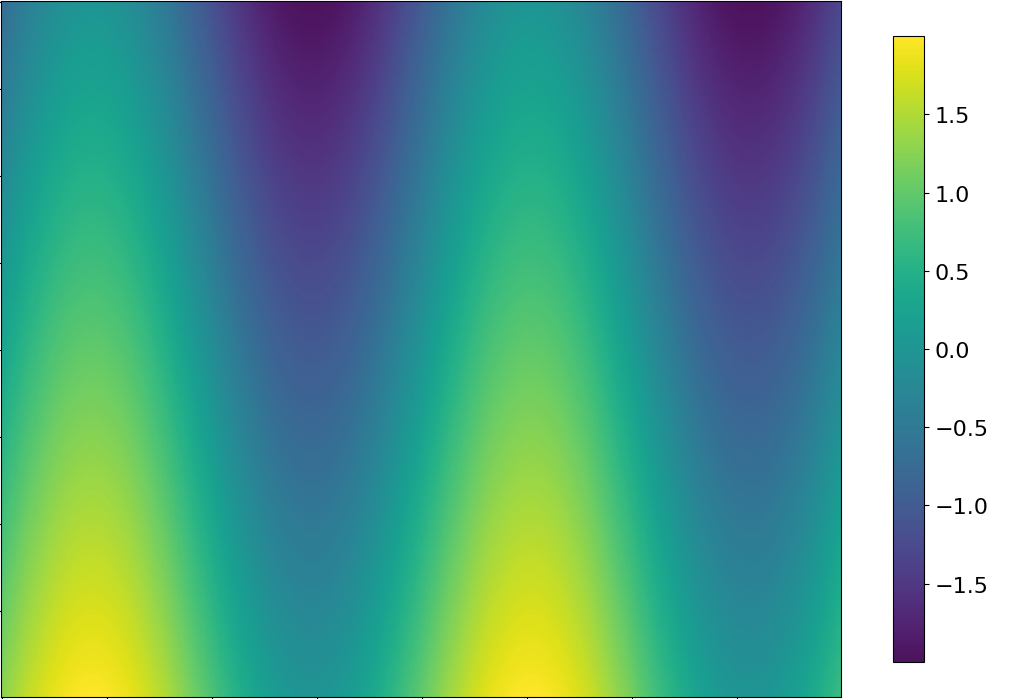
(a) Ground truth

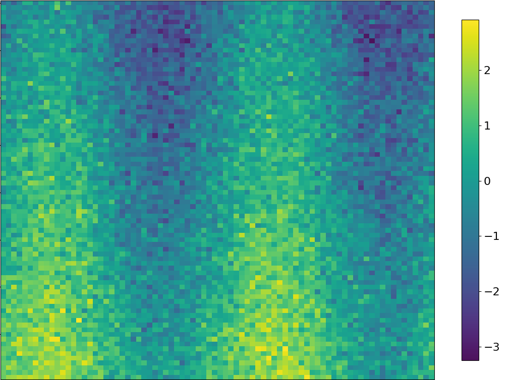
(b) Data

(c) Posterior mean

Figure 8: A demonstration of the performance of Algorithm 4 on a Gaussian process over two dimensions with randomly generated data. The data is defined on a square grid on $[-1,1]^{2}$ and $y_{i}=-x_{2,i}+\sin(6x_{1,i})+\epsilon_{i}$ where $\epsilon_{i}$ is IID Gaussian noise.

9 Conclusions

In this paper we introduce a class of numerical methods for converting a Gaussian process $f\sim\mathcal{GP}(0,k)$ on a user-defined rectangular region of $\mathbb{R}^{d}$ into a KL-expansion of the form

$$\hat{f}(x)=\alpha_{1}f_{1}(x)+...+\alpha_{m}f_{m}(x)$$ (9.1)

where $\alpha\sim\mathcal{N}(0,1)$ are IID and $f_{i}$ are fixed basis functions computed once during precomputation. The KL-expansion has several qualities that make it attractive for computationally demanding Gaussian process problems.

1. The KL-expansion is optimal in the $L^{2}$ sense. Specifically, for any order-$n$ basis function representation of a Gaussian process, the KL-expansion has an effective covariance kernel that best approximates the true kernel in the $L^{2}$ sense. This allows for highly accurate and compressed representations of Gaussian processes. For example, a Gaussian process on the interval $[-1,1]$ with squared exponential kernel

   $$k(x,x^{\prime})=\exp\bigg{(}-\frac{\|x-x^{\prime}\|^{2}}{2\ell^{2}}\bigg{)}$$ (9.2)

   with $\ell=0.1$, can be approximated to an accuracy of better than $10^{-3}$ with an expansion of $25$ basis functions.

2. KL-expansions can be computed directly and efficiently using well-known high-order algorithms for discretizing integral operators. For smooth kernels, convergence of these algorithms is super-algebraic. For kernels with $j$ continuous derivatives, convergence is no worse than $O(n^{-j-1})$ where $n$ is the number of discretization nodes.

3. Efficient statistical inference can be facilitated with KL-expansions. When viewed as a weight-space problem, the canonical Gaussian process regression is converted to a ridge regression in the space of expansion coefficients, where the number of coefficients is often significantly smaller than the number of data points. We also introduce an algorithm for rapidly evaluating posterior moments of Bayesian models.

The methods of this paper will likely generalize naturally to some families of non-Gaussian stochastic processes, such as stable distributions. A stable distribution is one where a linear combination of independent copies of the distribution follows the same distribution as the original, up to scale and location parameters Nolan, (2020). For example, suppose that we replace $\alpha_{1},...,\alpha_{m}$ in (9.1) with uncorrelated stable distributions such that

$$\mathbb{E}[\alpha_{i}]=0\qquad\text{and}\qquad\mathbb{E}[\alpha_{i}\alpha_{j}]=\delta_{ij}.$$ (9.3)

Then the KL-expansion

$$f(x)=\sum_{i=1}^{m}\alpha_{i}f_{i}(x)$$ (9.4)

is in the same family of distributions as the $\alpha_{i}$ and satisfies

$$\mathbb{E}[f(x)]=0\qquad\text{and}\qquad\mathbb{E}[f(x)f(y)]\approx k(x,y).$$ (9.5)

As a result, nearly all the numerical and analytical results of this paper generalize naturally to stable processes. Analytic and numerical investigations on this line of work are currently underway.

There are two main failure modes to the schemes of this paper. First, covariance kernels that are less smooth (i.e. they have more slowly decaying power spectra) require more terms in a KL-expansion for a given level of accuracy. Second, the methods of this paper suffer from the usual curse of dimensionality. For a given kernel of a Gaussian process over $\mathbb{R}^{d}$, the number of terms needed in a KL-expansion for a given level of accuracy grows like $m^{d}$ where $m$ is the number of terms required in one dimension. Due to these drawbacks, the numerical methods we describe are most useful in one and two dimensions, or in three-dimensional problems with smooth kernels.

10 Acknowledgements

The authors are grateful to Paul Beckman, Dan Foreman-Mackey, Jeremy Hoskins, Manas Rachh, and Vladimir Rokhlin for helpful discussions. The first author is supported by Alfred P. Sloan Foundation. The second author is supported in part by the Office of Naval Research under award numbers #N00014-21-1-2383 and the Simons Foundation/SFARI (560651, AB).

Appendix A Legendre polynomials

We now provide a brief overview of Legendre polynomials and Gaussian quadrature Abramowitz and Stegun, (1964). For a more in-depth analysis of these tools and their role in (numerical) approximation theory see, for example, Trefethen, (2020).

In accordance with standard practice, we denote by $P_{i}:[-1,1]\to\mathbb{R}$ the Legendre polynomial of degree $i$ defined by the three-term recursion

$$P_{i+1}(x)=\frac{2i+1}{i+1}\,x\,P_{i}(x)-\frac{i}{i+1}P_{i-1}(x)$$ (A.1)

with initial conditions

$$P_{0}(x)=1\qquad\text{and}\qquad P_{1}(x)=x.$$ (A.2)

Legendre polynomials are orthogonal on $[-1,1]$ and satisfy

$$\int_{-1}^{1}P_{i}(x)\,P_{j}(x)\,dx=\begin{cases}0&i\neq j,\\ \frac{2}{2i+1}&i=j.\end{cases}$$

We denote the $L^{2}$ normalized Legendre polynomials, $\overline{P}_{i}$, which are defined by

$$\overline{P}_{i}(x)=\sqrt{\frac{2i+1}{2}}P_{i}(x).$$ (A.3)

For each $n$, the Legendre polynomial $P_{n}$ has $n$ distinct roots which we denote in what follows by $x_{1},...,x_{n}$. Furthermore, for all $n$, there exist $n$ positive real numbers $w_{1},...,w_{n}$ such that for any polynomial $p$ of degree $\leq 2n-1$,

$$\int_{-1}^{1}p(x)\,dx=\sum_{i=1}^{n}w_{i}\,p(x_{i}).$$ (A.4)

The roots $x_{1},\ldots,x_{n}$ are usually referred to as order-$n$ Gaussian nodes and $w_{1},...,w_{n}$ the associated Gaussian quadrature weights. Classical Gaussian quadratures such as this are associated with many families of orthogonal polynomials: Chebyshev, Hermite, Laguerre, etc. The quadratures we mention above, associated with Legendre polynomials, provide a high-order method for discretizing (i.e. interpolating) and integrating square-integrable functions on a finite interval. Legendre polynomials are the natural orthogonal polynomial basis for square-integrable functions on the interval $[-1,1]$, and the associated interpolation and quadrature formulae provide nearly optimal approximation tools for these functions, even if they are not, in fact, polynomials.

The following well-known lemma regarding interpolation using Legendre polynomials will be used in the numerical schemes discussed in this paper. A proof can be found in Stoer and Bulirsch, (1992), for example.

Theorem A.1

Let $x_{1},...,x_{n}$ be the order-$n$ Gaussian nodes and $w_{1},...,w_{n}$ the associated order-$n$ Gaussian weights. Then there exists an $n\times n$ matrix $\bm{\mathsf{M}}$ that maps a function tabulated at these Gaussian nodes to the corresponding Legendre expansion, i.e. the interpolating polynomial expressed in terms of Legendre polynomials. That is to say, defining $\bm{\mathsf{f}}$ by

$$\bm{\mathsf{f}}=\left(f(x_{1})\cdots f(x_{n})\right)^{\mathsf{T}},$$ (A.5)

the vector

$$\bm{\mathsf{\alpha}}=\bm{\mathsf{M}}\bm{\mathsf{f}}$$ (A.6)

are the coefficients of the order-$n$ Legendre expansion $p$ such that

$$p(x_{j}) =\sum_{i=1}^{n}\alpha_{i}\,P_{i-1}(x_{j})$$ (A.7)

$$=f(x_{j}),$$

where $\alpha_{i}$ denotes the $i$th entry of the vector $\bm{\mathsf{\alpha}}$.

From a computational standpoint, algorithms for efficient evaluation of Legendre polynomials and Gaussian nodes and weights are available in standard software packages (e.g. Driscoll et al., (2014)). Furthermore, the entries of the matrix $\bm{\mathsf{M}}$ can be computed directly via $M_{i,j}=w_{j}P_{i-1}(x_{j})$.

References

- Abramowitz and Stegun, (1964) Abramowitz, M. and Stegun, I. A., editors (1964). Handbook of Mathematical Functions with Formulas, Graphs, and Mathematical Tables. National Bureau of Standards, Washington, D.C.
- Ambikasaran et al., (2016) Ambikasaran, S., Foreman-Mackey, D., Greengard, L., Hogg, D. W., and O’Neil, M. (2016). Fast Direct Methods for Gaussian Processes. IEEE Trans. Pattern Anal. Mach. Intell., 38(2):252–265.
- Baugh and Stein, (2018) Baugh, S. and Stein, M. L. (2018). Computationally efficient spatial modeling using recursive skeletonization factorizations. Spatial Statistics, 27:18–30.
- Carpenter et al., (2017) Carpenter, B., Gelman, A., Hoffman, M. D., Lee, D., Goodrich, B., Betancourt, M., Brubaker, M., Guo, J., Li, P., and Riddell, A. (2017). Stan: A probabilistic programming language. Journal of Statistical Software, Articles, 76(1):1–32.
- Cressie, (2015) Cressie, N. (2015). Statistics for Spatial Data, Revised Edition. Wiley-Interscience, Hoboken, NJ.
- Datta et al., (2016) Datta, A., Banerjee, S., Finley, A. O., and Gelfand, A. E. (2016). Hierarchical Nearest-Neighbor Gaussian Process Models for Large Geostatistical Datasets. J. Amer. Stat. Assoc., 111(514):800–812.
- Driscoll et al., (2014) Driscoll, T. A., Hale, N., and Trefethen, L. N. (2014). Chebfun Guide. Pafnuty Publications.
- Filip et al., (2019) Filip, S., Javeed, A., and Trefethen, L. N. (2019). Smooth Random Functions, Random ODEs, and Gaussian Processes. SIAM Review, 61(1):185–205.
- Foreman-Mackey et al., (2017) Foreman-Mackey, D., Agol, E., Ambikasaran, S., and Angus, R. (2017). Fast and Scalable Gaussian Process Modeling with Applications to Astronomical Time Series. The Astronomical Journal, 154(6).
- Gelman et al., (2013) Gelman, A., Carlin, J. B., Stern, H. S., Dunson, D. B., Vehtari, A., and Rubin, D. B. (2013). Bayesian Data Analysis. Chapman and Hall/CRC, New York, NY, 3rd edition.
- Gonzalvez et al., (2019) Gonzalvez, J., Lezmi, E., Roncalli, T., and Xu, J. (2019). Financial Applications of Gaussian Processes and Bayesian Optimization. arXiv, q-fin/1903.04841.
- Greengard et al., (2021) Greengard, P., Gelman, A., and Vehtari, A. (2021). A Fast Regression via SVD and Marginalization. Computational Statistics.
- Hastie et al., (2009) Hastie, T., Tibshirani, R., and Friedman, J. (2009). Elements of Statistical Learning. Springer Series in Statistics, New York, NY, 2nd edition.
- Kress, (1999) Kress, R. (1999). Linear Integral Equations. Springer, New York, NY.
- Lalchand and Rasmussen, (2020) Lalchand, V. and Rasmussen, C. E. (2020). Approximate inference for fully Bayesian Gaussian process regression. In Symposium on Advances in Approximate Bayesian Inference, pages 1–12. PMLR.
- Lázaro-Gredilla et al., (2010) Lázaro-Gredilla, M., Quiñnero-Candela, J., Rasmussen, C. E., and Figueiras-Vidal, A. R. (2010). Sparse spectrum gaussian process regression. Journal of Machine Learning Research, 11(63):1865–1881.
- Loève, (1977) Loève, M. (1977). Probability Theory I. Springer-Verlag, New York, NY.
- Minden et al., (2017) Minden, V., Damle, A., Ho, K. L., and Ying, L. (2017). Fast Spatial Gaussian Process Maximum Likelihood Estimation via Skeletonization Factorizations. Multiscale Modeling and Simulation, 15(4).
- Nolan, (2020) Nolan, J. P. (2020). Univariate Stable Distributions. Springer, New York, NY.
- Quinonero-Candela and Rasmussen, (2005) Quinonero-Candela, J. and Rasmussen, C. E. (2005). Analysis of some methods for reduced rank Gaussian process regression. In Switching and learning in feedback systems, pages 98–127. Springer.
- Rahimi and Recht, (2008) Rahimi, A. and Recht, B. (2008). Random features for large-scale kernel machines. In Platt, J., Koller, D., Singer, Y., and Roweis, S., editors, Advances in Neural Information Processing Systems, volume 20. Curran Associates, Inc.
- Rasmussen and Williams, (2006) Rasmussen, C. E. and Williams, C. L. I. (2006). Gaussian Processes for Machine Learning. MIT Press, Cambridge, MA.
- Riesz and Sz.-Nagy, (1955) Riesz, F. and Sz.-Nagy, B. (1955). Functional Analysis. Frederick Ungar Publishing Co., New York, NY.
- Riutort-Mayol et al., (2020) Riutort-Mayol, G., Bürkner, P.-C., Andersen, M. R., Solin, A., and Vehtari, A. (2020). Practical hilbert space approximate bayesian gaussian processes for probabilistic programming.
- Schwab and Todor, (2006) Schwab, C. and Todor, R. A. (2006). Karhunen–Loéve approximation of random fields by generalized fast multipole methods. J. Comput. Phys., 217:100–122.
- (26) Solin, A. and Särkkä, S. (2020a). Hilbert space methods for reduced-rank Gaussian process regression. Statistics and Computing, 30.
- (27) Solin, A. and Särkkä, S. (2020b). Hilbert space methods for reduced-rank gaussian process regression. https://github.com/AaltoML/hilbert-gp.
- Stoer and Bulirsch, (1992) Stoer, J. and Bulirsch, R. (1992). Introduction to Numerical Analysis. Springer-Verlag, New York, NY, 2nd edition.
- Trefethen, (2020) Trefethen, L. N. (2020). Approximation Theory and Approximation Practice: Extended Edition. SIAM, Philadelphia, PA.
- Xiu, (2010) Xiu, D. (2010). Numerical Methods for Stochastic Computations. Princeton University Press, Princeton, NJ.
- Yarvin and Rokhlin, (1998) Yarvin, N. and Rokhlin, V. (1998). Generalized Gaussian quadratures and singular value decompositions of integral operators. SIAM J. Sci. Comput., 20(2):699–720.