Anomalous dimensions of monopole operators at the transitions between Dirac and topological spin liquids

Abstract

Monopole operators are studied in a large family of quantum critical points between Dirac and topological quantum spin liquids (QSLs): chiral and $Z_{2}$ QSLs. These quantum phase transitions are described by conformal field theories (CFTs): quantum electrodynamics in 2+1 dimensions with $2N$ flavors of two-component massless Dirac fermions and a four-fermion interaction. For the transition to a chiral spin liquid, it is the Gross-Neveu interaction ($\operatorname{QED_{3}-GN}$), while for the transitions to $Z_{2}$ QSLs it is a superconducting pairing term with general spin/valley structure (generalized $\operatorname{QED_{3}-Z_{2}GN}$). Using the state-operator correspondence, we obtain monopole scaling dimensions to sub-leading order in $1/N$. For monopoles with a minimal topological charge $q=1/2$, the scaling dimension is $2N\times 0.26510$ at leading-order, with the quantum correction being $0.118911(7)$ for the chiral spin liquid, and $0.102846(9)$ for the simplest $Z_{2}$ case (the expression is also given for a general pairing term). Although these two anomalous dimensions are nearly equal, the underlying quantum fluctuations possess distinct origins. The analogous result in $\operatorname{QED_{3}}$ is also obtained and we find a sub-leading contribution of $-0.038138(5)$, which differs slightly from the value first obtained in the literature. The scaling dimension of a $\operatorname{QED_{3}-GN}$ monopole with minimal charge is very close to the scaling dimensions of other operators predicted to be equal by a conjectured duality between $\operatorname{QED_{3}-GN}$ with $2N=2$ flavors and the $\operatorname{CP}^{1}$ model. Additionally, non-minimally charged monopoles on both sides of the duality have similar scaling dimensions. By studying the large-$q$ asymptotics of the scaling dimensions in $\operatorname{QED_{3}}$, $\operatorname{QED_{3}-GN}$, and $\operatorname{QED_{3}-Z_{2}GN}$ we verify that the constant $O(q^{0})$ coefficient precisely matches the universal non-perturbative prediction for CFTs with a global $\operatorname{U}(1)$ symmetry.

I Introduction

Gauge theories play an important role in modern condensed matter physics, in part due to their ability to provide a low-energy description of many quantum phases of matter. Gauge fields emerge as collective excitations that capture the highly entangled nature of certain strongly correlated systems. This is notably apparent in the case of frustrated two-dimensional magnets hosting quantum spin liquids and deconfined quantum critical points (dQCPs).

In these lattice systems, the emergent gauge field is compact, and, as a result, has topological excitations created by topological disorder operators. For a $\operatorname{U}(1)$ gauge field, these objects are called monopole or instanton operators and they play an essential role in many physical systems. Crucially, monopole proliferation confines the gauge field. This is the case in the pure $\operatorname{U}(1)$ gauge theory [1; 2]. In the presence of massless matter, however, monopoles are screened and confinement can be avoided if enough flavors of massless matter are present.

In particular, we will be first considering a transition from a $\operatorname{U}(1)$ Dirac spin liquid (DSL), which is described by $\operatorname{QED_{3}}$ with $2N$ flavors of massless two-component Dirac fermions. Realizations of the $\operatorname{U}(1)$ DSL were formulated for the Kagome Heisenberg spin-$1/2$ magnet [3; 4; 5; 6; 7; 8] and the $J_{1}-J_{2}$ spin-$1/2$ model on the triangular lattice [9; 10; 11] with $2N=4$ flavors. Dirac spin-orbital liquid with effective spin $j=3/2$ and $2N=8$ flavors have also been formulated for quantum magnets on honeycomb [12; 13] and triangular [14] lattices. For a large number of fermion flavors $2N$, it has been shown through a $1/N$ expansion that monopole operators are irrelevant [15], and thus the $\operatorname{U}(1)$ DSL is stable in this limit. Taking into account next-to-leading order corrections [16], the critical number of fermion flavors was estimated to be $2N_{c}=12$, beyond which minimally charged monopoles become irrelevant. This result was confirmed by Monte Carlo computations [17] and is consistent with conformal bootstrap bounds [18; 19]. The addition of disorder renders the model more unstable [20].

Monopole operators also serve as order parameters in neighboring phases. For instance, in the $\operatorname{CP}^{1}$ model, which describes the transition between an antiferromagnetic (AFM) phase and a valence bond solid (VBS), there are monopoles with lattice quantum numbers and their condensation results in VBS order [21; 22; 23; 24]. It is in this model where the scaling dimension of monopole operators were first obtained [25]. Monopoles are also crucial in the $\operatorname{U}(1)$ DSL, a parent state for many spin liquids. In this fermionic theory, monopoles can carry different quantum numbers due to the existence of fermion zero modes [26] which may dress monopoles in various ways. Monopoles describe various VBS and AFM orders, depending on which lattice the $\operatorname{U}(1)$ DSL is formulated [27]. By tuning a flavor-dependent Gross-Neveu ($\operatorname{GN}$) interaction, a fermion mass is generated and monopoles with specific quantum numbers condense [28]. In particular, the $\operatorname{U}(1)$ DSL on the Kagome lattice orders to an antiferromagnetic $120^{\circ}$ coplanar order as monopoles dressed with a magnetic spin polarization condense [29; 30]. This confinement-deconfinement transition is described by the $\operatorname{QED_{3}}\!\operatorname{-}\!$ chiral Heisenberg $\operatorname{GN}$ model ($\operatorname{QED_{3}-cHGN}$), and the scaling dimensions of monopole operators at the quantum critical point (QCP) were obtained in Ref. [31]. In this case, the activation of the $\operatorname{cHGN}$ interaction breaks the flavor symmetry, resulting in a hierarchy among monopoles where the scaling dimension depends on the total magnetic spin of a monopole [32; 33].

The quantum criticality of the dQCP and the $\operatorname{U}(1)$ DSL with $2N=4$ fermions were recently given a precise relation. It was shown that they can be formulated as so-called Stiefel liquids, which are related to non-linear sigma models in $2+1$ dimensions with target manifolds $\operatorname{SO}\left(n\right)/\operatorname{SO}\left(4\right)$, where $n=5$ and $n=6$ for the dQCP and the $\operatorname{U}(1)$ DSL respectively [34]. Higher values are conjectured to realize non-lagrangian critical systems, for instance realizing a phase between a non-coplanar magnet and a VBS order when $n=7$.

In this work, we will focus on transitions from the $\operatorname{U}(1)$ DSL to two topological quantum spin liquids (QSL): a chiral spin liquid (CSL) as mentioned above, and a general type of $Z_{2}$ QSL. The first transition is described by $\operatorname{QED_{3}-GN}$ [35; 36], where the CSL results from the condensation of a symmetric fermion mass induced by the $\operatorname{GN}$ interaction. This transition can be realized for the Kagome [37; 38; 39; 40] and triangular [41; 42; 43] Heisenberg magnets with $2N=4$ Dirac cones. The QCP for the non-compact $\operatorname{QED_{3}-GN}$ has been studied in Refs. [36; 44; 45; 46; 47; 48]. Even though a mass gap is condensed in the CSL, there is no confinement-deconfinement transition taking place in the compact theory. Despite removing the screening effect of gapless modes, the symmetric condensed mass induces a Chern-Simons term in the infrared limit which gaps the monopoles and prevents their proliferation. The spinons in the gapped CSL thus remain deconfined. The CSL is a topologically ordered state that breaks time-reversal symmetry, and has robust chiral edge modes.

In contrast, the non-chiral $Z_{2}$ QSL is obtained when the fermionic spinons undergo a pairing instability to a gapped $s$-wave superconducting state. The U(1) gauge field is gapped through the Higgs mechanism, and gives place to a discrete $Z_{2}$ gauge field. In this case, fractionalization remains intact. For the simplest case where the pairing interaction is diagonal in flavor space, the corresponding quantum phase transition was studied in Refs. [49; 50]. Earlier studies [30; 51] qualitatively described how a Z₂ QSL can be obtained from a Dirac QSL through a superconducting transition for the fermions, albeit without a fluctuating scalar field (Cooper pair field). In addition, Ref. [52] studied a similar model in the context of superconducting criticality in topological insulators. Interestingly, it turns out that, at leading-order in $1/N$, the monopoles have the same scaling dimension at both QCPs as in the $\operatorname{U}(1)$ DSL [50; 31]. In this work, we obtain the next-to-leading order correction to monopole scaling dimensions at those QCPs. Futhermore, we also consider a more general class of $Z_{2}$ QSLs where the pairing interaction is not the same for all spin and valley degrees of freedom. We compute the anomalous dimension for the general $Z_{2}$ QSLs, and we also determine their bandstructure and Chern number inside the spin liquid phase.

This study is also motivated by the duality between $\operatorname{QED_{3}-GN}$ with $2N=2$ fermion flavors and $\text{CP}^{N-1}$ with $N=2$ complex boson flavors conjectured in Ref. [53] and further studied in Ref. [44]. This duality can be checked by comparing the scaling of monopole operators with various scaling dimensions that are predicted to be equal according to this duality. The good agreement obtained in the LO result [31] is further improved by the scaling dimension correction we obtain here for the $\operatorname{QED_{3}-GN}$ monopoles.

The paper is organized as follows. In the next section, we present the $\operatorname{QED_{3}-GN}$ model and show how the state-operator correspondence is used to obtain monopole scaling dimensions. In Sec. III, the leading-order computation presented in Ref. [31] is reviewed. In Sec. IV, $1/N$ corrections to monopole scaling dimensions are computed. We also verify that the scaling dimensions satisfy a conjectured convexity property. In Sec. V, we compare our results with the large-charge expansion obtained in Ref. [54] for CFTs. In Sec. VI, we study the $\operatorname{QED_{3}-GN}$ $\Leftrightarrow$ $\operatorname{CP}^{1}$ duality [53]. In Sec. VII, we study monopole scaling dimensions at the transition to a $Z_{2}$ QSL, and obtain distinct values compared to the CSL. In Sec. VIII, we briefly discuss other phase transitions that could be studied with this formalism, including the $\operatorname{QED_{3}}\!\operatorname{-}\!{\operatorname{U}(N)\times\operatorname{U}(N)}\operatorname{GN}$, $\operatorname{QED_{3}}\!\operatorname{-}\!\text{chiral XY}\operatorname{GN}$, and $\operatorname{QED_{3}-cHGN}$ QCPs. We conclude with a discussion of our results and an outlook. In Appendix A, we review the phase transition from the $\operatorname{U}(1)$ DSL to the CSL in the non-compact model. In Apps. B and C, we give more details regarding how the kernels appearing in Sec. IV are obtained and simplified with gauge invariance. The expansion of these kernels in terms of harmonics is detailed in Apps. D and E. We give detailed simplifications of the kernels used for the case of minimally charge monopoles in App. F. In App. G, some remainder coefficients used to analytically approximate sums over angular momenta are shown. In App. H, we show how some contributions of fermion zero modes neglected in the main text vanish. In App. I, the fitting procedure used to alleviate finite-size effects when computing monopole anomalous dimensions are described. In App. J, we list monopole anomalous dimensions in $\operatorname{QED_{3}}$, $\operatorname{QED_{3}-GN}$, and $\operatorname{QED_{3}-Z_{2}GN}$ for topological charges up to $q=13$.

II Monopoles at transition between Dirac & chiral spin liquids

The action of the $\operatorname{QED_{3}-GN}$ model in euclidean flat spacetime is given by

$$S=\!\int\!d^{3}r\left[-\overline{\Psi}\gamma^{\mu}\left(\partial_{\mu}-iA_{\mu}\right)\Psi-\frac{h^{2}}{2}\left(\overline{\Psi}\Psi\right)^{2}\right]+\dotsb,$$ (2.1)

where $\Psi$ is a $2N$ flavor spinor $\Psi=\left(\psi_{1},\psi_{2},\dots\psi_{2N}\right)^{\intercal}$with each flavor $\psi_{i}$ being a two-component Dirac fermion. For certain quantum magnets, where fermions emerge as fractionalized quasiparticles, the $2N$ flavors are related to two magnetic spin polarizations $s=\uparrow,\downarrow$ and $N$ valley nodes per spin, $v=1,\dots,N$. Typical quantum magnets have $N=2$ or $4$ nodes, but here we keep $N$ general and use it as an expansion parameter. The adjoint spinor is given by $\overline{\Psi}=\Psi^{\dagger}\gamma_{0}$, where the gamma matrices are defined in terms of the Pauli matrices by $\gamma_{x,y}=\sigma_{x,y}$, and $\gamma_{0}=\sigma_{z}$. The fermions are coupled to a compact $\operatorname{U}(1)$ gauge field $A_{\mu}$, and have a $\operatorname{GN}$ self-interaction with coupling strength $h$. The ellipsis denotes an irrelevant Maxwell term and the contribution of monopole operators $\mathcal{M}_{q}(x)$ that we discuss further in what follows.

In $2+1$ dimensions, $\operatorname{U}(1)$ gauge theories have an extra global $\operatorname{U}_{\text{top}}(1)$ symmetry associated with the following conserved current

$$J_{\text{top}}^{\mu}(x)=\frac{1}{2\pi}\epsilon^{\mu\nu\rho}\partial_{\nu}A_{\rho}(x),$$ (2.2)

where “top” stands for topological. The operators charged under $\operatorname{U}_{\text{top}}(1)$ are called topological disorder operators or instantons. In this $2+1$ dimensional context, we refer to them as monopole operators. These operators create topological configurations of the gauge field $\mathcal{A}_{\mu}^{q}$ with a quantized flux $\int dn_{\mu}\epsilon^{\mu\nu\rho}\partial_{\nu}\mathcal{A}_{\rho}^{q}=4\pi q$, where the topological charge is a half-integer $q\in\mathbb{Z}/2$ as a result of the Dirac quantization condition [55]. These kinds of configurations are allowed in the compact formulation of the $\operatorname{U}(1)$ gauge group, which gives the correct description for emergent gauge theories in a condensed matter context. The monopole operators themselves can be defined by the action of the topological current on them:

$$J_{\text{top}}^{\mu}(x)\mathcal{M}_{q}^{\dagger}(0)\sim\frac{q}{2\pi}\frac{x^{\mu}}{\left|x\right|^{3}}\mathcal{M}_{q}^{\dagger}(0)+\cdots,$$ (2.3)

where the ellipsis denotes less singular terms in the operator-product expansion ($\operatorname{OPE}$) [15]. The resulting factor in front of the monopole operator corresponds to the magnetic field of a charge-$q$ Dirac magnetic monopole.

The model in Eq. (2.1) describes a transition from a DSL to a CSL. For a sufficiently strong coupling, a chiral order develops due to the condensation of a fermion bilinear: $\langle\overline{\Psi}\Psi\rangle\neq 0$. This may be studied by introducing an auxiliary pseudo-scalar boson $\phi$. The effective action at the quantum critical point (QCP), denoted by $S_{\operatorname{eff}}^{\text{c}}$, is

$$S_{\operatorname{eff}}^{\text{c}}=-2N\ln\det(\not{\partial}-i\not{A}+\phi),$$ (2.4)

where $\phi$ is an auxiliary boson decoupling the $\operatorname{GN}$ interaction. More details are shown in App. A.

In the compact version of $\operatorname{QED_{3}-GN}$, monopole operators are also present at the QCP. The main goal of this paper is to compute their scaling dimension $\Delta_{\mathcal{M}_{q}}$ , which controls the scaling of the monopole two-point correlation function:

$$\langle\mathcal{M}_{q}(x)\mathcal{M}_{q}^{\dagger}(y)\rangle\sim\frac{1}{\left|x-y\right|^{2\Delta_{\mathcal{M}_{q}}}}.$$ (2.5)

Since the $\operatorname{QED_{3}-GN}$ model at the QCP is a conformal field theory ($\operatorname{CFT}$), the state-operator correspondence can be used to obtain these scaling dimensions [15]. This correspondence relies on a radial quantization of the $\operatorname{CFT}$ and a conformal transformation mapping the dilatation operator $\hat{D}$ on $\mathbb{R}^{3}$ to a Hamiltonian $\hat{H}$ on $S^{2}\times\mathbb{R}$. Denoting the usual radius on $\mathbb{R}^{3}$ as $r=e^{\tau}$, the related Weyl transformation of the spacetime is written as

$$\left(ds^{2}\right)_{S^{2}\times\mathbb{R}} =e^{-2\tau}\left(ds^{2}\right)_{\mathbb{R}^{3}}=d\tau^{2}+d\theta^{2}+\sin^{2}\theta d\phi^{2}.$$ (2.6)

The scaling dimension of an operator $\mathcal{O}(x)$ then corresponds to the energy of some state $\hat{H}\left|\mathcal{O}\right\rangle=\Delta_{\mathcal{O}}\left|\mathcal{O}\right\rangle$ on this compactified spacetime. Specifically, the charge-$q$ operator with the smallest scaling dimension corresponds to the ground state of the $\operatorname{CFT}$ on the compactified spacetime $S^{2}\times\mathbb{R}$, where the sphere $S^{2}$ is pierced by $4\pi q$ flux. To implement this flux, an external gauge field is coupled to the fermions

$$\mathcal{A}^{q}=q\left(1-\cos\theta\right)\mathrm{d}\phi,$$ (2.7)

or $\mathcal{A}_{\phi}^{q}=\left(1-\cos\theta\right)/\sin\theta$ in component notation. The smallest scaling dimension of monopole operators in topological sector $q$ is then given by

$$\Delta_{q} =\lim_{\beta\to\infty}F_{q}=-\lim_{\beta\to\infty}\frac{1}{\beta}\ln Z\left[\mathcal{A}^{q}\right],$$ (2.8)

where $F_{q}$ is the free energy and $Z\left[\mathcal{A}^{q}\right]$ is the partition function formulated on $S^{2}\times S_{\beta}^{1}$, i.e., the previous spacetime but now with the “time” direction compactified to a “thermal” circle $S_{\beta}^{1}$ with radius $\beta$. This formulation allows us to introduce the holonomy of the gauge field along this circle, written as

$$\alpha=i\beta^{-1}\int_{S_{\beta}^{1}}d\tau\ A_{\tau}.$$ (2.9)

The holonomy couples to the fermion number operator $\int d^{2}r\sqrt{g(r)}\Psi^{\dagger}\Psi=\hat{N}_{\text{fermions}}$ and acts as a chemical potential [19; 31]. The saddle-point equation of this holonomy constrains the fermion number to vanish

$$0=\frac{1}{\beta}\left.\frac{\delta\ln Z\left[\mathcal{A}^{q}\right]}{\delta\alpha}\right|_{\text{s.p.}}=\bigl{\langle}\hat{N}_{\text{fermions}}\bigr{\rangle},$$ (2.10)

where “s.p.” stands for saddle-point. The holonomy thus serves as a Lagrange multiplier that ensures that a state with $\langle\hat{N}_{\text{fermions}}\rangle=0$ is selected to correctly represent a gauge-invariant monopole operator [31].

The scaling dimension will be obtained using a large-$N$ expansion. We first note that the partition function can be written as a path integral:

$$Z\left[\mathcal{A}^{q}\right]=e^{-\beta F_{q}}=\int\mathcal{D}\phi\mathcal{D}A_{\mu}\exp\left(-S_{\operatorname{eff}}\left[\phi,A_{\mu},\mathcal{A}_{\mu}^{q}\right]\right).$$ (2.11)

The effective action is now given by

$$S_{\operatorname{eff}}\left[\phi,A_{\mu},\mathcal{A}_{\mu}^{q}\right]= -2N\ln\det\left(\not{D}_{A+\mathcal{A}^{q}}+\phi\right),$$ (2.12)

where $\not{D}_{A+\mathcal{A}^{q}}$ is the gauge-covariant derivative on a curved spacetime including the external gauge field $\mathcal{A}_{\mu}^{q}$ sourcing the $4\pi q$ flux:

$$\not{D}_{A+\mathcal{A}^{q}}=e_{b}^{\mu}\gamma^{b}\left(\nabla_{\mu}-iA_{\mu}-i\mathcal{A}_{\mu}^{q}\right).$$ (2.13)

The gamma matrices $\gamma^{b}$ still correspond to the Pauli matrices, as the spacetime index is normalized with a tetrad $e^{\mu}_{b}$ which encapsulates the information about the metric $g_{\mu\nu}e^{\mu}_{b}e^{\nu}_{c}=\delta_{bc}$. The path integral defining the partition function can be expanded around the saddle-point values of the auxiliary and gauge bosons:

$$\phi=\langle\phi\rangle+\sigma,\quad A_{\mu}=\langle A_{\mu}\rangle+a_{\mu},$$ (2.14)

which are defined by the following saddle-point conditions

$$\left.\frac{\delta F_{q}}{\delta\phi}\right|_{\phi=\langle\phi\rangle,A_{\mu}=\langle A_{\mu}\rangle}=\left.\frac{\delta F_{q}}{\delta A_{\mu}}\right|_{\phi=\langle\phi\rangle,A_{\mu}=\langle A_{\mu}\rangle}=0.$$ (2.15)

Taking the fluctuations to scale as $1/\sqrt{2N}$, the saddle-point expansion of the partition function is then

$$\int\mathcal{D}\phi\mathcal{D}Ae^{-S_{\operatorname{eff}}}=e^{-\left.S_{\operatorname{eff}}\right|_{\text{s.p.}}}\int\mathcal{D}\sigma\mathcal{D}ae^{-S_{\operatorname{eff}}^{(2)}},$$ (2.16)

where $S_{\operatorname{eff}}^{\left(2\right)}$ is the second variation of the action. Integrating over the quadratic fluctuations, this gives us the $1/N$ expansion of the free energy:

$$2NF_{q}^{(0)} =\frac{1}{\beta}\left.S_{\operatorname{eff}}\right|_{\text{s.p.}},$$ (2.17)

$$F_{q}^{(1)} =\frac{1}{\beta}\times\frac{1}{2}\left.\ln\det\left[\frac{\delta^{2}S_{\operatorname{eff}}}{\delta\left(\sigma,a\right)\delta\left(\sigma,a\right)}\right]\right|_{\text{s.p.}}.$$ (2.18)

Using the relation in Eq. (2.8), which follows from the state-operator correspondence, these first two terms of the free energy give the scaling dimension at next-to-leading order in $1/N$.

Since the fermionic mass condensed in the ordered phase is flavor-symmetric $\left\langle\overline{\Psi}\Psi\right\rangle$, the global flavor symmetry remains unbroken and monopole operators are organized as representations of $\operatorname{SU}(2N)$. Just as for the various fermion bilinears and monopole correlation functions in the $\operatorname{U}(1)$ DSL [57; 58; 29], monopole correlation functions at the QCP between $\operatorname{U}(1)$ DSL and CSL related by this $\operatorname{SU}(2N)$ symmetry share the same scaling dimension. Depending on the lattice, various magnetic and VBS correlation functions will be described by minimally charged monopole operators [27], but they all share the same scaling dimension $2N\times 0.26510+0.118911(7)+O\left(N^{-1}\right)$, where the leading-order was found in Ref. [31] and the next-to-leading order is one of the main results of this work shown in Eq. (4.61). For typical quantum magnets, we have $2N=4$ fermion flavors. The way that monopole scaling dimensions control observable correlation functions could also be compared at this QCP and deep in the $\operatorname{U}(1)$ DSL phase. In this latter case, scaling dimensions are those of monopoles in $\operatorname{QED_{3}}$.

III Review of $N=\infty$ theory

First, we review the computation of monopole scaling dimensions in $\operatorname{QED_{3}-GN}$ at leading-order in $1/N$ [31]. At this order, the free energy is given by the effective action in (2.12) at its saddle-point corresponding to a global minimum

$$F_{q}^{(0)}=-\frac{1}{\beta}\ln\det\left(\not{D}_{-i\alpha d\tau+\mathcal{A}^{q}}+\left\langle\phi\right\rangle\right),$$ (3.1)

where the trace over the $2N$ flavors has been taken and has canceled a prefactor of $(2N)^{-1}.$ The expectation value of the pseudo-scalar field is taken to be homogeneous. The gauge field is also constant at the saddle-point, with a possible non-vanishing holonomy $\alpha$ on the thermal circle described in (2.9). The determinant operator is diagonalized by introducing monopole harmonics $Y_{q,\ell,m}(\hat{n})$, which are a generalization of spherical harmonics for a space with a charge at the center [59; 60]. For a fixed charge $q$, these functions form a complete basis. One important difference with these harmonics is that their angular momentum is now bounded below by this charge $q$. Using these functions to build appropriate eigenspinors, the eigenvalues of this determinant operator on $S^{2}\times S_{\beta}^{1}$ in Eq. (3.1) are shown to be [15; 31]

$$-i\times\begin{cases}\omega_{n}-i\alpha+i\varepsilon_{q}&\ell=q,\\ \pm\sqrt{\left(\omega_{n}-i\alpha\right)^{2}+\varepsilon_{\ell}^{2}}&\ell=q+1,q+2,\dots\end{cases}$$ (3.2)

where, for simplicity, we suppose $q>0$ throughout. Here, $\omega_{n}=2\pi\beta^{-1}\left(n+1/2\right)$, for $n\in\mathbb{Z}$, are the fermionic Matsubara frequencies, and $\varepsilon_{\ell}$ are the energies of the modes for the quantized theory on $S^{2}\times\mathbb{R}$:

$$\varepsilon_{\ell} =\sqrt{\ell^{2}-q^{2}+\langle\phi\rangle^{2}}.$$ (3.3)

More details on the diagonalization are presented in App. (D.2). Note that the energies are dimensionless, as we work in units where the radius of the sphere is $1$. Each mode has the usual degeneracy that comes from the azimuthal symmetry, $d_{\ell}=2\ell$. The free energy at leading-order then becomes

$$\begin{split}F_{q}^{(0)}&=-\frac{1}{\beta}\sum_{n=-\infty}^{\infty}\biggl{\{}d_{q}\ln\left[\omega_{n}-i\alpha+i\left\langle\phi\right\rangle\right]\\ &\quad{}+\sum_{\ell=q+1}^{\infty}d_{\ell}\ln\left[\left(\omega_{n}-i\alpha\right)^{2}+\varepsilon_{\ell}^{2}\right]\biggr{\}}.\end{split}$$ (3.4)

The saddle-point equation for the holonomy, given in Eq. (2.15), yields the condition

$$-d_{q}\tanh\left(\frac{\beta}{2}(\alpha-\left\langle\phi\right\rangle)\right)-\sum_{\ell=q+1}^{\infty}\frac{2d_{\ell}\sinh\left(\beta\alpha\right)}{\cosh\left(\beta\varepsilon_{\ell}\right)+\cosh\left(\beta\alpha\right)}=0,$$ (3.5)

which is solved for $\alpha=\left\langle\phi\right\rangle$ in the $\beta\to\infty$ limit. With this result, the second gap equation at leading-order in $\beta$ is given by

$$2\left\langle\phi\right\rangle\sum_{\ell=q+1}^{\infty}d_{\ell}\varepsilon_{\ell}^{-1}=0,$$ (3.6)

whose only solution is $\left\langle\phi\right\rangle=0$. Therefore, the saddle-point values of both fields vanish.

Inserting this result in Eq. (3.4), the monopole scaling dimension at leading-order in $1/N$ is obtained from Eq. (2.8)

$$\Delta_{q}=2N\sum_{\ell=q+1}^{\infty}d_{\ell}E_{q,\ell}+O\left(N^{0}\right),$$ (3.7)

where the energies at the saddle-point are defined as

$$E_{q,\ell}=\sqrt{\ell^{2}-q^{2}}.$$ (3.8)

This is simply the leading-order scaling dimension of $\operatorname{QED_{3}}$ [15] (which must still be regularized). For example, the scaling dimension of the monopole with minimal charge is $\Delta_{q=1/2}=2N\times 0.265+O\left(N^{0}\right)$. Here, a supplementary $\operatorname{GN}$ interaction is considered, but it does not come into play at this level of the expansion since $\langle\phi\rangle=0$. Thus, monopoles in $\operatorname{QED_{3}}$ and $\operatorname{QED_{3}-GN}$ have the same scaling dimensions at leading-order in $1/N$:

$$\Delta_{q,\operatorname{QED_{3}}}^{(0)}=\Delta_{q,\operatorname{QED_{3}-GN}}^{(0)}.$$ (3.9)

IV $1/N$ corrections

IV.1 Setup

IV.1.1 Real-space kernels

We now turn to the next-to-leading-order term in the free-energy expansion in Eq. (2.18). The free-energy correction is related to the second variation of the action by

$$\begin{split}\exp\left(-\beta F_{q}^{(1)}\right)=&\int\mathcal{D}\sigma\mathcal{D}a\exp\left[-\frac{\left(2N\right)}{2}\int_{r,r^{\prime}}\begin{pmatrix}\sigma(r)&a_{\mu}(r)\end{pmatrix}\right.\\ &\times\left.\begin{pmatrix}D^{q}(r,r^{\prime})&H_{\mu^{\prime}}^{q}(r,r^{\prime})\\ H_{\mu}^{q}\left(r^{\prime},r\right)&K_{\mu\mu^{\prime}}^{q}(r,r^{\prime})\end{pmatrix}\begin{pmatrix}\sigma\left(r^{\prime}\right)\\ a_{\mu^{\prime}}\left(r^{\prime}\right)\end{pmatrix}\right],\end{split}$$ (4.1)

where $\int_{r}\equiv\int d^{3}r\sqrt{g(r)}$ and we defined the following kernels

$$D^{q}(r,r^{\prime}) =\frac{1}{2N}\left.\frac{\delta^{2}S_{\operatorname{eff}}}{\delta\sigma(r)\delta\sigma\left(r^{\prime}\right)}\right|_{\text{s.p.}},$$ (4.2)

$$K_{\mu\mu^{\prime}}^{q}(r,r^{\prime}) =\frac{1}{2N}\left.\frac{\delta^{2}S_{\operatorname{eff}}}{\delta a^{\mu}(r)\delta a^{\mu^{\prime}}\left(r^{\prime}\right)}\right|_{\text{s.p.}},$$ (4.3)

$$H_{\mu^{\prime}}^{q}(r,r^{\prime}) =\frac{1}{2N}\left.\frac{\delta^{2}S_{\operatorname{eff}}}{\delta\sigma(r)\delta a^{\mu^{\prime}}\left(r^{\prime}\right)}\right|_{\text{s.p.}},$$ (4.4)

where $S_{\operatorname{eff}}$ is defined in Eq. (2.12). The remaining scalar-gauge kernel with mixed $a_{\mu}(r)$ and $\sigma\left(r^{\prime}\right)$ partial derivatives is obtained by exchanging coordinates $r,r^{\prime}$ in $H_{\mu^{\prime}}^{q}(r,r^{\prime})$, which has mixed $\sigma(r)$ and $a_{\mu^{\prime}}\left(r^{\prime}\right)$ partial derivatives; thus we write $H_{\mu}^{q}\left(r^{\prime},r\right)$ in Eq. (4.1). In terms of the fermions in the original system, the kernels are given by

$$D^{q}(r,r^{\prime}) =\left.\left\langle\overline{\psi}(r)\psi(r)\overline{\psi}\left(r^{\prime}\right)\psi\left(r^{\prime}\right)\right\rangle\right|_{\text{s.p.}},$$ (4.5)

$$K_{\mu\mu^{\prime}}^{q}(r,r^{\prime}) =-\left.\bigl{\langle}J_{\mu}(r)J_{\mu^{\prime}}\left(r^{\prime}\right)\bigr{\rangle}\right|_{\text{s.p.}},$$ (4.6)

$$H_{\mu^{\prime}}^{q}(r,r^{\prime}) =-i\left.\bigl{\langle}\overline{\psi}(r)\psi(r)J_{\mu^{\prime}}\left(r^{\prime}\right)\bigr{\rangle}\right|_{\text{s.p.}},$$ (4.7)

where $\psi$ is a single fermion flavor and the current is

$$J_{\mu}(r)=\overline{\psi}(r)\gamma_{\mu}\psi(r).$$ (4.8)

This can be re-expressed in terms of the fermionic Green’s function $G_{q}(r,r^{\prime})=\left.\left\langle\psi(r)\overline{\psi}\left(r^{\prime}\right)\right\rangle\right|_{\text{s.p.}}$ and its hermitian conjugate $G_{q}^{\dagger}(r,r^{\prime})=-\left.\left\langle\psi\left(r^{\prime}\right)\overline{\psi}(r)\right\rangle\right|_{\text{s.p.}}$. The Wick expansion of the kernels yields

$$D^{q}(r,r^{\prime}) =-\text{tr}\left[G_{q}(r,r^{\prime})G_{q}^{\dagger}(r,r^{\prime})\right],$$ (4.9)

$$K_{\mu\mu^{\prime}}^{q}(r,r^{\prime}) =\text{tr}\left[\gamma_{\mu}G_{q}(r,r^{\prime})\gamma_{\mu^{\prime}}G_{q}^{\dagger}(r,r^{\prime})\right],$$ (4.10)

$$H_{\mu^{\prime}}^{q}(r,r^{\prime}) =i\text{tr}\left[G_{q}(r,r^{\prime})\gamma_{\mu^{\prime}}G_{q}^{\dagger}(r,r^{\prime})\right],$$ (4.11)

where the cyclicity of the trace was used. The remaining prefactor $2N$ in Eq. (4.1) is cancelled as the fluctuation fields are rescaled $\sigma,a_{\mu}\to\sigma/\sqrt{2N},a_{\mu}/\sqrt{2N}$ to control the expansion. The free-energy correction is then obtained by integrating the field fluctuations in Eq. (4.1). It is convenient to subtract the $q=0$ correction $F_{0}^{(1)}=0$, therefore we write the general correction as

$$F_{q}^{(1)}=\frac{1}{2}\ln\left(\frac{\det^{\prime}M^{q}}{\det^{\prime}M^{0}}\right),$$ (4.12)

where we define the matrix kernel

$$M^{q}(r,r^{\prime})=\left(\begin{array}[]{cc}D^{q}(r,r^{\prime})&H_{\mu^{\prime}}^{q}(r,r^{\prime})\\ H_{\mu}^{q}\left(r^{\prime},r\right)&K_{\mu\mu^{\prime}}^{q}(r,r^{\prime})\end{array}\right).$$ (4.13)

IV.1.2 Fourier transform

To compute the determinant operator, the kernels are expanded in terms of harmonics. For the gauge-gauge kernels, the vector spherical harmonics are introduced:

$$\mathfrak{a}_{\mu,\ell m}^{T}(\hat{n}) =\delta_{\mu}^{0}Y_{\ell m}(\hat{n}),$$ (4.14)

$$\mathfrak{a}_{\mu,\ell m}^{E}(\hat{n}) =\frac{1}{\sqrt{\ell(\ell+1)}}\nabla_{\mu}Y_{\ell m}(\hat{n}),$$ (4.15)

$$\mathfrak{a}_{\ell m}^{\mu,B}(\hat{n}) =\frac{1}{\sqrt{\ell(\ell+1)}}\frac{\epsilon^{0\mu\nu}}{\sqrt{g(r)}}\nabla_{\nu}Y_{\ell m}(\hat{n}).$$ (4.16)

As suggested by the notation, the $B$ mode has zero divergence: $\nabla\cdot\vec{\mathfrak{a}}_{\ell m}^{B}(\hat{n})=0$, and the $E$ mode has zero curl: $\nabla\boldsymbol{\times}\vec{\mathfrak{a}}_{\ell m}^{E}(\hat{n})=0$. It is also useful to introduce 4-dimensional eigenfunctions,

$$\mathbb{Y}_{\ell m}^{D}(\hat{n}) =\begin{pmatrix}Y_{\ell m}(\hat{n})\\ 0^{\mu}\end{pmatrix},\quad\mathbb{Y}_{\ell m}^{X}(\hat{n})=\begin{pmatrix}0\\ \mathfrak{a}_{\ell m}^{\mu,X}(\hat{n})\end{pmatrix},$$ (4.17)

where $X\in\{T,E,B\}$. In this basis, the matrix kernel $M^{q}(r,r^{\prime})$ can be expanded as

$$M^{q}(r,r^{\prime}) =\int_{-\infty}^{\infty}\frac{d\omega}{2\pi}\sum_{\ell=0}^{\infty}\sum_{m=-\ell}^{\ell}e^{-i\omega(\tau-\tau^{\prime})}$$ (4.18)

$$\quad{}\times\begin{pmatrix}\mathbb{Y}_{\ell m}^{D}(\hat{n})\\ \mathbb{Y}_{\ell m}^{T}(\hat{n})\\ \mathbb{Y}_{\ell m}^{E}(\hat{n})\\ \mathbb{Y}_{\ell m}^{B}(\hat{n})\end{pmatrix}^{\intercal}M_{\ell}^{q}(\omega)\begin{pmatrix}\mathbb{Y}_{\ell m}^{D}(\hat{n}^{\prime})^{\dagger}\\ \mathbb{Y}_{\ell m}^{T}(\hat{n}^{\prime})^{\dagger}\\ \mathbb{Y}_{\ell m}^{E}(\hat{n}^{\prime})^{\dagger}\\ \mathbb{Y}_{\ell m}^{B}(\hat{n}^{\prime})^{\dagger}\end{pmatrix},$$

where we directly work on $S^{2}\times\mathbb{R}$ (i.e., taking the limit $\beta\to\infty$ now) and where

$$M_{\ell}^{q}(\omega)=\begin{pmatrix}D_{\ell}^{q}&H_{\ell}^{q,T}&H_{\ell}^{q,E}&H_{\ell}^{q,B}\\ -H_{\ell}^{q,T*}&K_{\ell}^{q,TT}&K_{\ell}^{q,TE}&K_{\ell}^{q,TB}\\ -H_{\ell}^{q,E*}&K_{\ell}^{q,TE*}&K_{\ell}^{q,EE}&K_{\ell}^{q,EB}\\ -H_{\ell}^{q,B*}&K_{\ell}^{q,TB*}&K_{\ell}^{q,EB*}&K_{\ell}^{q,BB}\end{pmatrix}.$$ (4.19)

All of the arguments of the functions appearing in the matrix are $\omega$. Note that the scalar-gauge kernel is imaginary, hence the reason for the signs in the first column of the matrix. This last point is shown explicitly in App. B.

This kernel can be simplified by using $\mathcal{CT}$ invariance. The auxiliary boson $\phi$, a pseudo-scalar, and the $E,T$ modes of the gauge field are antisymmetric under $\mathcal{CT}$, while the $B$ modes are symmetric under $\mathcal{CT}$. This implies that the following kernels vanish

$$K_{\ell}^{q,TB}(\omega) =K_{\ell}^{q,EB}(\omega)=H_{\ell}^{q,B}(\omega)=0.$$ (4.20)

The $\operatorname{U}(1)$ gauge invariance also enables the kernel to be simplified. Using the conservation of the $\operatorname{U}(1)$ current, $\nabla_{\mu}J^{\mu}(r)=0$, in Eqs. (4.6-4.7), it follows that

$$K_{\ell}^{q,TE}(\omega) =\frac{i\omega}{\sqrt{\ell(\ell+1)}}K_{\ell}^{q,TT}(\omega),$$ (4.21)

$$K_{\ell}^{q,EE}(\omega) =\frac{\omega^{2}}{\ell(\ell+1)}K_{\ell}^{q,TT}(\omega),$$ (4.22)

$$H_{\ell}^{q,E}(\omega) =\frac{i\omega}{\sqrt{\ell(\ell+1)}}H_{\ell}^{q,T}(\omega).$$ (4.23)

It should also be noted that among vector spherical harmonics, only $\mathfrak{a}_{\mu,\ell m}^{T}(\hat{n})$ is defined for $\ell=0.$ In this case, the only remaining gauge-gauge kernel is $K_{0}^{q,TT}(\omega)$, and it vanishes by gauge invariance. The computations to obtain these gauge invariance conditions are shown in App. C. Using all these simplifications, the monopole scaling dimension correction is given by

$$\Delta_{q,\operatorname{QED_{3}-GN}}^{(1)} =\frac{1}{2}\int_{\omega}\left\{\ln\left(\frac{D_{0}^{q}(\omega)}{D_{0}^{0}(\omega)}\right)+\sum_{\ell=1}^{\infty}\left(2\ell+1\right)\ln\left[\dfrac{K_{\ell}^{q,B}(\omega)\left(D_{\ell}^{q}(\omega)K_{\ell}^{q,E}(\omega)+\left(1+\frac{\omega^{2}}{\ell(\ell+1)}\right)\left|H_{\ell}^{q,T}(\omega)\right|^{2}\right)}{K_{\ell}^{0,B}(\omega)D_{\ell}^{0}(\omega)K_{\ell}^{0,E}(\omega)}\right]\right\},$$ (4.24)

where $\int_{\omega}\equiv\int_{-\infty}^{\infty}d\omega/\left(2\pi\right)$ and we defined

$$K_{\ell}^{q,E}(\omega) \equiv K_{\ell}^{q,TT}(\omega)+K_{\ell}^{q,EE}(\omega),$$ (4.25)

$$K_{\ell}^{q,B}(\omega) \equiv K_{\ell}^{q,BB}(\omega).$$ (4.26)

Note that $H_{\ell}^{0,T}(\omega)=0$ and thus it does not appear in the denominator.

By turning off the $\operatorname{GN}$ interaction in Eq. (4.24), the scalar-scalar kernel $D_{\ell}^{q}(\omega)$ and the scalar-gauge kernel $H_{\ell}^{q,T}(\omega)$ do not contribute, and the monopole scaling dimension correction in $\operatorname{QED_{3}}$ [16] is recovered:

$$\Delta_{q,\operatorname{QED_{3}}}^{(1)}=\frac{1}{2}\int_{\omega}\sum_{\ell=1}^{\infty}\left(2\ell+1\right)\ln\left[\dfrac{K_{\ell}^{q,B}(\omega)K_{\ell}^{q,E}(\omega)}{K_{\ell}^{0,B}(\omega)K_{\ell}^{0,E}(\omega)}\right],$$ (4.27)

One can alternatively deactivate the gauge field, keeping only the scalar-scalar kernels, and obtain the pure $\operatorname{GN}$ model. Despite the absence of a gauge field in this model, one can still introduce an external gauge field with the $4\pi q$ flux, define a correlation function on this background configuration, and obtain the related critical exponent. This was notably achieved for the $\operatorname{O}(N)$ model in Ref. [62]. In a forthcoming publication, we shall also explore this avenue in the pure-$\operatorname{GN}$ model.

The relevant kernel Fourier coefficients to compute the monopole scaling dimensions in (4.24) and (4.27) are found by inverting Eq. (4.18):

$$D_{\ell}^{q}(\omega) =\frac{4\pi}{2\ell+1}\int_{r}e^{i\omega\tau}D^{q}\left(r,0\right)\sum_{m}Y_{\ell m}^{*}(\hat{n})Y_{\ell m}\left(\hat{z}\right),$$ (4.28)

$$H_{\ell}^{q,T}(\omega) =\frac{4\pi}{2\ell+1}\int_{r}e^{i\omega\tau}H_{0}^{q}\left(r,0\right)\sum_{m}Y_{\ell m}^{*}(\hat{n})Y_{\ell m}\left(\hat{z}\right),$$ (4.29)

$$K_{\ell}^{q,E}(\omega) =\frac{4\pi}{2\ell+1}\int_{r}e^{i\omega\tau}\bigg{[}K_{00}^{q}\left(r,0\right)\sum_{m}Y_{\ell m}^{*}(\hat{n})Y_{\ell m}\left(\hat{z}\right)$$

$${}\quad+K_{aa^{\prime}}^{q}\left(r,0\right)\sum_{m}\mathfrak{a}_{\ell m}^{a,E*}(\hat{n})\mathfrak{a}_{\ell m}^{a^{\prime},E}\left(\hat{z}\right)\bigg{]},$$ (4.30)

$$K_{\ell}^{q,B}(\omega) =\frac{4\pi}{2\ell+1}\int_{r}e^{i\omega\tau}K_{aa^{\prime}}^{q}\left(r,0\right)\sum_{m}\mathcal{\mathfrak{a}}_{\ell m}^{a,B*}(\hat{n})\mathcal{\mathfrak{a}}_{\ell m}^{a^{\prime},B}\left(\hat{z}\right),$$ (4.31)

where the second coordinates are fixed to $\tau^{\prime}=0$ and $\hat{n}^{\prime}=\hat{z}$ without loss of generality, and normalized coordinates $a,a^{\prime}$ are introduced.

IV.2 Anomalous dimensions

The anomalous dimensions of monopole operators (4.24, 4.27) are computed in this section. To do so, the kernel coefficients in Eqs. (4.28, 4.30, 4.31) must be obtained. These coefficients are built with real-space kernels (4.9-4.11) that depend on the fermionic Green’s function at the saddle-point. The Green’s function is defined by the action of the Dirac operator on it:

$$i\not{D}_{\mathcal{A}^{q}}^{S^{2}\times\mathbb{R}}(r)G_{q}(r,r^{\prime})=-\delta(r-r^{\prime}).$$ (4.32)

The eigenkernels in Eqs. (4.28, 4.30, 4.31), involving the sums on spherical harmonics or vector spherical harmonics, will also be needed.

IV.2.1 $q=0$ kernels

We first compute the expressions in the denominator of the scaling-dimension corrections (4.24, 4.27), that is, the $q=0$ kernel coefficients. The eigenkernel in the scalar-scalar kernel (4.28) is just the sum of spherical harmonics, which is given by the addition theorem

$$\sum_{m}Y_{\ell m}^{*}(\hat{n})Y_{\ell m}(\hat{n}^{\prime})=\frac{2\ell+1}{4\pi}P_{\ell}\left(\cos\gamma\right),$$ (4.33)

where

$$\cos\gamma\equiv\hat{n}\cdot\hat{n}^{\prime}=\cos\theta\cos\theta^{\prime}+\sin\theta\sin\theta^{\prime}\cos\left(\phi-\phi^{\prime}\right).$$ (4.34)

When working with $\hat{n}^{\prime}=\hat{z}$, this is replaced by

$$x\equiv\cos\theta.$$ (4.35)

For the sums on vector spherical harmonics appearing in the gauge-gauge kernels (4.30, 4.31), a similar result is obtained in spherical coordinates $a=\hat{\theta},\text{$\hat{\phi},\hat{\tau}$}$ in Eqs. (E.4, E.5) in App. E and is formulated with the same Legendre polynomial and its first and second derivatives. This reproduces a result from Ref. [63].

The real-space kernel for $q=0$ is also needed. In this case, the Green’s function takes a simple form which is simply the conformally transformed $3D$ flat space Green’s function [16]:

$$G_{0}\left(\tau-\tau^{\prime},\hat{n},\hat{n}^{\prime}\right)=\frac{i}{4\pi X^{3}}\vec{\gamma}\cdot\left(e^{\frac{1}{2}(\tau-\tau^{\prime})}\hat{n}-e^{-\frac{1}{2}(\tau-\tau^{\prime})}\hat{n}^{\prime}\right),$$ (4.36)

where

$$X\equiv[2\cosh(\tau-\tau^{\prime})-2\cos\gamma]^{1/2}.$$ (4.37)

The real-space kernels can then be obtained in normalized spherical coordinates. Inserting this Green’s function, along with the eigenkernels, in Eqs. (4.28, 4.30, 4.31), the resulting $q=0$ kernel coefficients are (setting $\tau^{\prime}=0$)

$$D_{\ell}^{0}(\omega) =-\frac{1}{8\pi^{2}}\int_{r}e^{i\omega\tau}P_{\ell}(x)\frac{1}{X^{4}},$$ (4.38)

$$K_{\ell}^{0,E}(\omega) =\frac{1}{32\pi^{2}}\int_{r}e^{i\omega\tau}P_{\ell}(x)\Big{(}-\nabla_{S^{2}}^{2}$$

$$\quad+\frac{1}{\ell(\ell+1)}\nabla_{S^{2}}^{2}\partial_{\tau}^{2}\Big{)}\frac{1}{X^{2}},$$ (4.39)

$$K_{\ell}^{0,B}(\omega) =\frac{1}{16\pi^{2}\ell(\ell+1)}\int_{r}e^{i\omega\tau}P_{\ell}(x)\nabla_{S^{2}}^{2}\frac{1}{X^{4}},$$ (4.40)

where integration by parts was used to eliminate derivatives of $P_{\ell}(x)$. The differential operators acting on $e^{i\omega\tau}P_{\ell}(x)$ can be replaced with the corresponding eigenvalues $\nabla_{S^{2}}^{2}\to-\ell(\ell+1)$ and $\partial_{\tau}^{2}\to-\omega^{2}$ with further integration by parts. The remaining expressions contain Fourier transforms of the form $\int_{r}e^{i\omega\tau}P_{\ell}(x)X^{p}$ which were obtained in the appendix of Ref. [63]. Using these results, the $q=0$ kernel coefficients are simplified to

$$D_{\ell}^{0}(\omega) =\left(\ell^{2}+\omega^{2}\right)\mathcal{D}_{\ell-1}(\omega),$$ (4.41)

$$K_{\ell}^{0,E}(\omega) =\frac{1}{2}\left(\ell(\ell+1)+\omega^{2}\right)\mathcal{D}_{\ell}(\omega),$$ (4.42)

$$K_{\ell}^{0,B}(\omega) =\frac{1}{2}\left(\ell^{2}+\omega^{2}\right)\mathcal{D}_{\ell-1}(\omega),$$ (4.43)

where

$$\mathcal{D}_{\ell}(\omega)=\left|\frac{\Gamma\left(\frac{1+\ell+i\omega}{2}\right)}{4\Gamma\left(\frac{2+\ell+i\omega}{2}\right)}\right|^{2}.$$ (4.44)

Note that we have reproduced the gauge-gauge coefficients $K_{\ell}^{0,E}(\omega)$ and $K_{\ell}^{0,B}(\omega)$ given in Ref. [16] by using the methods of Ref. [63].

IV.2.2 Anomalous dimensions for $q=1/2$

For the minimal magnetic charge, the eigenkernels in Eqs. (4.28-4.31) are formulated using the same expression (4.33, E.4, E.5) as in the last section. In particular, the gauge-gauge kernels will be worked out in normalized spherical coordinates. As for the real-space kernels (4.9-4.11), they depend on the $q=1/2$ fermionic Green’s function defined through Eq. (4.32). The spectral decomposition of the Green’s function in terms of spinors with monopole harmonics components is shown in App. D.2. A generalized addition theorem for monopole harmonics involving the Jacobi Polynomials $P_{\ell}^{\left(0,2q\right)}(x)$ is then needed. Specifically, after taking the sum over the azimuthal quantum number, the Green’s function for general $q$ is given by [16]

$$\begin{split}G_{q}\left(\tau,\hat{n};\tau^{\prime},\hat{n}^{\prime}\right)&=\frac{i}{2}e^{-i2q\Theta}\sum_{\ell=q}^{\infty}e^{-E_{q,\ell}\left|\tau-\tau^{\prime}\right|}\left\{-\dfrac{E_{q,\ell}}{1-x}Q_{q,\ell}(x)\left(\hat{n}-\hat{n}^{\prime}\right)\cdot\vec{\gamma}\right.\\ &\quad{}\left.+\text{sgn}(\tau-\tau^{\prime})\left[qQ_{q,\ell}(x)\mathbb{I}+Q^{\prime}_{q,\ell}(x)\left(\hat{n}+\hat{n}^{\prime}\right)\cdot\vec{\gamma}+i\dfrac{q}{1+x}Q_{q,\ell}(x)\left(\hat{n}\times\hat{n}^{\prime}\right)\cdot\vec{\gamma}\right]\right\},\end{split}$$ (4.45)

where the energies $E_{q,\ell}$ were defined in Eq. (3.8) and where

$$Q_{q,\ell}(x)=\dfrac{\left(1+x\right)^{q}}{\left(4\pi\right)2^{q}}\begin{cases}P_{\ell-q}^{\left(0,2q\right)}(x)-P_{\ell-1-q}^{\left(0,2q\right)}(x),&\ell>q,\\ 1,&\ell=q.\end{cases}$$ (4.46)

The phase $e^{-i2q\Theta}$ comes from the generalized addition theorem and is defined in Eq. (D.23), but it is not involved in the computation since it is always cancelled by the opposite phase of the Green’s function hermitian conjugate. The Green’s function can be inserted in Eqs. (4.9-4.11) to obtain the real-space kernels, which, along with the eigenkernels (4.33, E.4, E.5), are inserted in Eqs. (4.28-4.31) to compute the four kernel coefficients. Defining $K_{\ell}^{q,D}(\omega)\equiv D_{\ell}^{q}(\omega)$ and $K_{\ell}^{q,T}(\omega)\equiv H_{\ell}^{q,T}(\omega)$, the kernel coefficients $K_{\ell}^{q,Z}(\omega)$ with $Z\in\{D,T,E,B\}$ are given by

$$K_{\ell}^{q,Z}(\omega) =\sum_{\ell^{\prime},\ell^{\prime\prime}}\frac{4\pi A^{Z}\bigl{(}E_{q,\ell^{\prime}}+E_{q,\ell^{\prime\prime}}\bigr{)}}{\omega^{2}+\bigl{(}E_{q,\ell^{\prime}}+E_{q,\ell^{\prime\prime}}\bigr{)}^{2}}\biggl{[}\frac{\mathcal{I}_{1}^{Z}}{2}+E_{q,\ell^{\prime}}E_{q,\ell^{\prime\prime}}\mathcal{I}_{2}^{Z}\biggr{]}$$

$$\equiv\sum_{\ell^{\prime},\ell^{\prime\prime}}^{\infty}k_{\ell,\ell^{\prime},\ell^{\prime\prime}}^{q,Z}(\omega),$$ (4.47)

where the prefactors are given by

$$A^{Z}=\Bigl{\{}1,i,\tfrac{1}{\ell(\ell+1)},\tfrac{1}{\ell(\ell+1)}\Bigr{\}},\ Z\in\{D,T,E,B\},$$ (4.48)

the integrals for scalar-scalar and scalar-gauge kernels are

$$\mathcal{I}_{1}^{D} =-2\int dxP_{\ell}\Big{[}q^{2}\frac{1}{1+x}Q_{q,\ell^{\prime}}Q_{q,\ell^{\prime\prime}}$$

$$\quad{}+\left(1+x\right)Q^{\prime}{}_{q,\ell^{\prime}}Q^{\prime}{}_{q,\ell^{\prime\prime}}\Big{]},$$ (4.49)

$$\mathcal{I}_{2}^{D} =-\int dx\frac{1}{1-x}P_{\ell}Q_{q,\ell^{\prime}}Q_{q,\ell^{\prime\prime}},$$ (4.50)

$$\mathcal{I}_{1}^{T} =-2q\int dxP_{\ell}^{\prime}Q_{q,\ell^{\prime}}Q_{q,\ell^{\prime\prime}},$$ (4.51)

$$\mathcal{I}_{2}^{T} =0,$$ (4.52)

and the integrals for gauge-gauge kernels reproduce the expressions obtained in Ref. [16]

$$\mathcal{I}_{1}^{E} =2\int dx\left\{\left[\frac{2\ell(\ell+1)P_{\ell}+\left(1-x\right)P_{\ell}^{\prime}}{1+x}\right]q^{2}Q_{q,\ell^{\prime}}Q_{q,\ell^{\prime\prime}}\right.$$

$$\quad{}\left.-\left(1-x^{2}\right)P_{\ell}^{\prime}Q^{\prime}{}_{q,\ell^{\prime}}Q^{\prime}{}_{q,\ell^{\prime\prime}}\right\},$$ (4.53)

$$\mathcal{I}_{2}^{E} =-\int dx\left(\frac{1+x}{1-x}\right)P_{\ell}^{\prime}Q_{q,\ell^{\prime}}Q_{q,\ell^{\prime\prime}},$$ (4.54)

$$\mathcal{I}_{1}^{B} =2\int dx\left\{\left[P_{\ell}^{\prime}-\left(1-x\right)P_{\ell}^{\prime\prime}\right]\right.\left[q^{2}Q_{q,\ell^{\prime}}Q_{q,\ell^{\prime\prime}}\right.$$

$$\quad{}\left.\left.-\left(1+x\right)^{2}Q^{\prime}{}_{q,\ell^{\prime}}Q^{\prime}{}_{q,\ell^{\prime\prime}}\right]\right\},$$ (4.55)

$$\mathcal{I}_{2}^{B} =\int dx\left[P_{\ell}^{\prime}+\left(1+x\right)P_{\ell}^{\prime\prime}\right]Q_{q,\ell^{\prime}}Q_{q,\ell^{\prime\prime}}.$$ (4.56)

These integrals can be performed exactly, see App. F for more details. In the end, these quantities depend only on the angular momenta: $\mathcal{I}_{1}^{Z}\left(\ell,\ell^{\prime},\ell^{\prime\prime}\right)$ and $\mathcal{I}_{2}^{Z}\left(\ell,\ell^{\prime},\ell^{\prime\prime}\right)$. For $\ell^{\prime}=\ell^{\prime\prime}=q$, this computation requires more care since both energies vanish, and the integral over time leading to the prefactor in Eq. (4.47) instead yields a Dirac delta function $\delta(\omega)$. However, for $\ell^{\prime}=\ell^{\prime\prime}=q=1/2$, the term in the bracket simply vanishes. When only one of $\ell^{\prime}$ and $\ell^{\prime}$ have their minimal value $q=1/2$, there is a non-vanishing contribution to the anomalous dimension. In this case, only $\mathcal{I}_{1}^{Z}$ contributes, since the prefactor in front of $\mathcal{I}_{2}^{Z}$ in Eq. (4.47) vanishes. For $q=1/2$, the contribution of zero modes in Eq. (4.47) vanishes with $\ell=\omega=0$, otherwise it is given by

$$2\sum_{\ell^{\prime}=3/2}^{\infty}k_{\ell,\ell^{\prime},1/2}^{1/2,Z}(\omega)=-\frac{1}{4\pi}\frac{\sqrt{\ell(\ell+1)}}{\omega^{2}+\ell(\ell+1)}\times\{1,-i,0,1\}.$$ (4.57)

The remaining contribution consists in a sum on non-zero modes $\ell^{\prime},\ell^{\prime\prime}\geq 3/2$. The summand depends on $\mathcal{I}_{1}^{Z}\left(\ell,\ell^{\prime},\ell^{\prime\prime}\right)$ and $\mathcal{I}_{2}^{Z}\left(\ell,\ell^{\prime},\ell^{\prime\prime}\right)$ which are formed of three-$J$ symbols in $\ell,\ell^{\prime}$ and $\ell^{\prime\prime}$ (F.6-F.8). Thus, one of the sums, say on $\ell^{\prime\prime}$, can be viewed as finite. Then, after taking the sum on $\ell^{\prime\prime}$, the remaining summand tends to a constant for large $\ell^{\prime}$

$$\lim_{\ell^{\prime}\to\infty}\sum_{\ell^{\prime\prime}=3/2}^{\infty}k_{\ell,\ell^{\prime},\ell^{\prime\prime}}^{1/2,Z}(\omega)=\alpha^{Z}=-\frac{1}{4\pi}\times\{2,0,1,1\}.$$ (4.58)

Thus, for kernels with a non-zero asymptotic constant, the sum on $\ell^{\prime}$ will be divergent. This is regularized with a zeta function regularization $\sum_{\ell=a}^{\infty}\ell^{-p}=\zeta\left(p,a\right)$, here specifically $\zeta\left(0,3/2\right)=-1$

$$-\alpha^{Z}+\sum_{\ell^{\prime}=3/2}^{\infty}\biggl{[}-\alpha^{Z}+\sum_{\ell^{\prime\prime}=3/2}^{\infty}k_{\ell,\ell^{\prime},\ell^{\prime\prime}}^{1/2,Z}(\omega)\biggr{]}.$$ (4.59)

The sum above is then finite and is computed numerically up to a cutoff $\ell_{c}^{\prime}$. The remainder is approximated with a large $\ell^{\prime}$ expansion of the summand $-\alpha^{Z}+\sum_{\ell^{\prime\prime}}k_{\ell,\ell^{\prime},\ell^{\prime\prime}}^{1/2,Z}(\omega)=\sum_{p=2}^{k}c_{\ell,p}^{1/2,Z}(\omega)\left(\ell^{\prime}\right)^{-p}+O\left(1/\ell^{\prime\left(k+1\right)}\right)$. Each power in the expansion is summed analytically from $\ell^{\prime}=\ell_{c}^{\prime}+1$ to $\ell^{\prime}=\infty$ with a zeta function. The coefficients $c_{\ell,p}^{1/2,Z}(\omega)$ are found by doing the expansion for a few fixed values of $\ell$ and deducing the general dependence on $\ell$. It turns out that only even powers of $1/\ell^{\prime}$ have non-vanishing coefficients $\text{$c_{\ell,p}^{1/2,Z}(\omega)$}.$ We obtained the expansion up to $k=18$. With this remainder, we found that a cutoff $\ell_{c}^{\prime}=300+1/2$ was sufficiently large to achieve the desired precision goals. The first few terms of the remainders for general $q$ are shown in App. G.

After performing the sums in Eqs. (4.57, 4.59), the kernel coefficients in Eq. (4.47) are computed and inserted in Eq. (4.24) (or Eq. (4.27) for the case of $\operatorname{QED_{3}}$). The kernel coefficients in the denominator of the logarithm of the monopole anomalous dimension were obtained analytically in Eqs. (4.41-4.43). The remaining sum on $\ell$ and integral on $\omega$ are computed up to a relativistic cutoff [16]

$$\ell(\ell+1)+\omega^{2}\leq L\left(L+1\right).$$ (4.60)

We obtained the anomalous dimension with a cutoff up to $L_{\max}=65$. A function of $1/L$ is then fitted to extract the value of the anomalous dimension as the full sum and integration are taken with $L\to\infty$. Fig. 1 shows a quartic function fitted with the data from $L\in[L_{\max}-10,L_{\max}]$. The anomalous dimension of a charge $q=1/2$ monopole in $\operatorname{QED_{3}-GN}$ extracted from this fit is $\Delta_{1/2,\operatorname{QED_{3}-GN}}^{(1)}=0.11890$, whereas in $\operatorname{QED_{3}}$ it is given by $\Delta_{1/2,\operatorname{QED_{3}}}^{(1)}=-0.03814$. This reproduces the result in Ref. [16] up to a difference of order $10^{-4}$.

While we extrapolated the result for $L\to\infty$ with a quartic fit, based on a cutoff of $L_{\max}=65$, varying the maximal relativistic cutoff can change the last digit in the result quoted above. For instance, $\Delta_{1/2,\operatorname{QED_{3}}}^{(1)}|_{L_{\max}=50}=-0.03815$. In App. I, we show how we computed anomalous dimensions for various $L_{\max}$ and used the trend as $L_{\max}\to\infty$ to estimate the anomalous dimensions and their errors. The error we quote in what follows reflects the uncertainties related to the extrapolations and not the precision of our computation which yields relatively negligible errors.

Using this method, the anomalous dimension of $q=1/2$ monopoles at next-to-leading order in the $1/N$ expansion in $\operatorname{QED_{3}-GN}$ is given by

$$\Delta_{1/2,\operatorname{QED_{3}-GN}}^{(1)} =0.118911(7).$$ (4.61)

The scaling dimension of $q=1/2$ monopole operators in $\operatorname{QED_{3}-GN}$ is then given by $2N\times 0.26510+0.118911(7)+O\left(N^{-1}\right)$. In $\operatorname{QED_{3}}$, the correction we found is

$$\Delta_{1/2,\operatorname{QED_{3}}}^{(1)}=-0.038138(5).$$ (4.62)

With this estimated uncertainty of our result, it is clearer that there is a small discrepancy when comparing our result with the correction $-0.0383$ computed in Ref. [16]. Trying to replicate the method in Ref. [16], we used a cubic fit with data $L\in[5,45]$ and obtained $-0.03823$, which is closer to $-0.0383$.

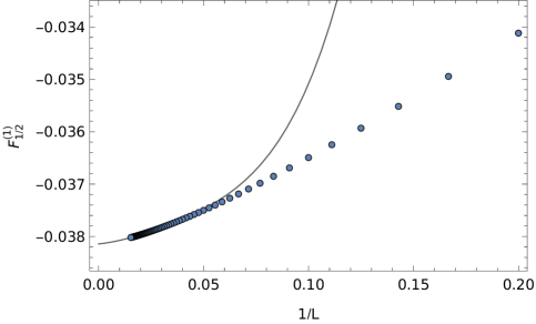
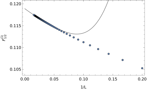
Figure 1: Anomalous dimension of the $q\!=\!1/2$ monopole $\Delta_{1/2}^{(1)}$ (4.24, 4.27) as a function of the relativistic cutoff $L$ (4.60) in (a) $\operatorname{QED_{3}}$ ; (b) $\operatorname{QED_{3}-GN}$. The points are obtained by numerically computing Eqs. (4.24, 4.27), and the solid line is a quartic fit in $1/L$ with the points $L\in[55,65]$.

IV.2.3 Anomalous dimensions for general $q$

For larger topological charge $q$, many results used from App. F are not easily generalized. In the previous section, the computations involved three different Jacobi polynomials that appear after taking the sum over an appropriate azimuthal quantum number. Here instead, the real-space kernels and the eigenkernels will be written explicitly as sums of monopole spherical harmonics, respectively with finite charge $q$ and vanishing charge. This follows the alternative and more algorithmic method presented in Ref. [61].

For the real-space kernels, the required formulation already appears as an intermediate step in App. D.2 when obtaining the Green’s function in Eq. (4.45). The Green’s function is a $2\times 2$ matrix acting on particle-hole space with components given by the product of two monopole harmonics (D.20-D.22). Consequently, the real-space kernels are formulated as products of four monopole harmonics. As for the eigenkernels appearing in $D_{\ell}^{q}(\omega)$, $H_{\ell}^{q,T}(\omega)$, they are already expressed as the product of two spherical harmonics (4.28, 4.29). Only the gauge-gauge kernels then need a reformulation. In this case, a different basis $U_{\ell,m}^{\mu}(\hat{n}),V_{\ell,m}^{\mu}(\hat{n}),W_{\ell,m}^{\mu}(\hat{n})$ for the vector spherical harmonics can be introduced. These are eigenfunctions with respective total spin $j=\ell-1,\ell$ and $\ell+1$ [16]. Most importantly, the components of these harmonics are simply given by spherical harmonics (see App. E.2). We discuss the relation with the previous basis shortly.

Before doing so, we note that, in this new formulation, the kernel coefficients are expressed as the integral of a product of four monopole harmonics and two spherical harmonics. To be more precise, half of these functions are conjugate harmonics, but they can all be expressed as harmonics with the following relation

$$Y_{q,\ell,m}^{*}(\hat{n})=\left(-1\right)^{q+m}Y_{-q,\ell,-m}(\hat{n}).$$ (4.63)

Just as we did in Sec. IV.2, the primed coordinates can be fixed as $\tau^{\prime}=0$ and $\hat{n}^{\prime}=\hat{z}$ without loss of generality. As a result, half of the six harmonics are eliminated

$$Y_{q,\ell,m}\left(\hat{z}\right) =\delta_{q,-m}\sqrt{\frac{2\ell+1}{4\pi}}.$$ (4.64)

This removes every sum on azimuthal quantum numbers, which greatly simplifies the computation. There remains an integral over three harmonics

$$\begin{split}\int d\hat{n}Y_{q,\ell,m}(\hat{n})Y_{q^{\prime},\ell^{\prime},m^{\prime}}(\hat{n})Y_{q^{\prime\prime},\ell^{\prime\prime},m^{\prime\prime}}(\hat{n})=\left(-1\right)^{\ell+\ell^{\prime}+\ell^{\prime\prime}}\\ \times\sqrt{\frac{\left(2\ell+1\right)\left(2\ell^{\prime}+1\right)\left(2\ell^{\prime\prime}+1\right)}{4\pi}}\begin{pmatrix}\ell&\ell^{\prime}&\ell^{\prime\prime}\\ q&q^{\prime}&q^{\prime\prime}\end{pmatrix}\begin{pmatrix}\ell&\ell^{\prime}&\ell^{\prime\prime}\\ m&m^{\prime}&m^{\prime\prime}\end{pmatrix}.\end{split}$$ (4.65)

The explicit expressions for the kernel coefficients involve the sum of many such integrals and are not reproduced here.

Returning to the change of basis, the $U,V,W$ vector spherical harmonics in the $j=\ell$ sector can be related to the harmonics previously introduced in Eqs. (4.14-4.16) by

$$\begin{pmatrix}U_{\ell+1,m}^{\mu}(\hat{n})\\ W_{\ell-1,m}^{\mu}(\hat{n})\\ V_{\ell,m}^{\mu}(\hat{n})\end{pmatrix} =\begin{pmatrix}-\sqrt{\frac{\ell+1}{2\ell+1}}&\sqrt{\frac{\ell}{2\ell+1}}&0\\ \sqrt{\frac{\ell}{2\ell+1}}&\sqrt{\frac{\ell+1}{2\ell+1}}&0\\ 0&0&i\end{pmatrix}\begin{pmatrix}\mathfrak{a}_{\ell m}^{T,\mu}(\hat{n})\\ \mathfrak{a}_{\ell m}^{E,\mu}(\hat{n})\\ \mathfrak{a}_{\ell m}^{B,\mu}(\hat{n})\end{pmatrix}$$

$$\equiv\mathcal{R}\begin{pmatrix}\mathfrak{a}_{\ell m}^{T,\mu}(\hat{n})\\ \mathfrak{a}_{\ell m}^{E,\mu}(\hat{n})\\ \mathfrak{a}_{\ell m}^{B,\mu}(\hat{n})\end{pmatrix}.$$ (4.66)

The Fourier coefficients can also be transformed in this basis:

$$\begin{split}\mathcal{R}\begin{pmatrix}K_{\ell}^{q,TT}(\omega)&K_{\ell}^{q,TE}(\omega)&0\\ K_{\ell}^{q,TE*}(\omega)&K_{\ell}^{q,EE}(\omega)&0\\ 0&0&K_{\ell}^{q,BB}(\omega)\end{pmatrix}\mathcal{R}^{-1}\\ =\begin{pmatrix}K_{\ell}^{q,UU}(\omega)&K_{\ell}^{q,UW}(\omega)&0\\ K_{\ell}^{q,UW*}(\omega)&K_{\ell}^{q,WW}(\omega)&0\\ 0&0&K_{\ell}^{q,VV}(\omega)\end{pmatrix}.\end{split}$$ (4.67)

The matrix of eigenkernels keeps the same structure thanks to the block-diagonal form of the transformation matrix $\mathcal{R}$. This is expected, as we could also argue that the kernels $K_{\ell}^{q,UV}(\omega)=K_{\ell}^{q,WV}(\omega)=0$ vanish because of $CT$ invariance, as we did for $K_{\ell}^{q,TB}(\omega)=K_{\ell}^{q,EB}(\omega)=0$. The relevant relations are then

$$K_{\ell}^{q,VV}(\omega) =K_{\ell}^{q,B}(\omega),$$ (4.68)

$$K_{\ell}^{q,UU}(\omega)+K_{\ell}^{q,WW}(\omega) =K_{\ell}^{q,E}(\omega).$$ (4.69)

The first relation is found by comparing the bottom-right components in Eq. (4.67) and using the definition of $K_{\ell}^{q,B}(\omega)$ (4.26), whereas the second relation is found by taking the trace of Eq. (4.67), using the first result in Eq. (4.68) and the definition of $K_{\ell}^{q,E}(\omega)$ (4.25). The kernels $K_{\ell}^{q,E}(\omega)$ and $K_{\ell}^{q,B}(\omega)$ can then be replaced in the scaling-dimension corrections (4.24-4.27) by their formulation in the new basis.

For general charge, the regularization of the kernels presented in Eqs. (4.58, 4.59) is still valid : Regulator terms $-1/\left(2\pi\right)$ and $-1/\left(4\pi\right)$ can be used respectively for the scalar-scalar and gauge-gauge kernels, while the scalar-gauge kernel does not require regularization. The contribution of the zero modes using this method is also very straightforward and algorithmic. However, there seems to be additional contributions coming from the combination of zero modes in both Green’s function, $\ell^{\prime}=\ell^{\prime\prime}=q$. As discussed previously, this contribution is proportional to a Dirac Delta function $\delta(\omega)$ instead of the energy prefactor in Eq. (4.47). This contribution vanishes once integrated over $\omega$ (see App. H). Numerical sums on $\ell^{\prime}$ are obtained up to $\ell_{c}^{\prime}=200+q$, and the remainder is computed analytically with an expansion up to $1/\ell^{\prime 18}$. In this case, the coefficients of the expansion also depend on the charge $q$ and are found by fixing $\ell$ and $q$ for a few values.

The anomalous dimension $\Delta_{q}^{(1)}$ for each charge are computed with a relativistic cutoff $L_{\max}=35+\lfloor q\rceil$, where $\lfloor q\rceil\equiv\text{Round}(q)$. Here, the convention is that half-integers are rounded to even numbers, e.g. $\lfloor 1/2\rceil=0$ and $\lfloor 3/2\rceil=2$. The value of $L_{\max}$ is modulated with the charge $q$ to ensure that a regime with a tail-like behaviour, as observed in Fig. 1, is attained for larger charges. For the three minimal charges, we used a larger relativistic cutoff: We use $L_{\max}=65$ for $q=1/2$ (as in the last section) and $L_{\max}=46,47$ for $q=1,3/2$. We found that the results are robust as $L_{\max}$ is increased and more precise (see App. I). The results for $L\in[L_{\max}-6,L_{\max}]$ are used to fit a quartic function in $1/L$ to extrapolate the anomalous dimensions $\Delta_{q}^{(1)}$ as $L\to\infty$. The fits obtained for $q=5/2$ monopoles in $\operatorname{QED_{3}}$ and $\operatorname{QED_{3}-GN}$ are shown in Fig. 2 and yield scaling-dimension corrections $\Delta_{5/2,\operatorname{QED_{3}}}^{(1)}=-1.0359$ and $\Delta_{5/2,\operatorname{QED_{3}-GN}}^{(1)}=0.6253$ as $L\to\infty$.

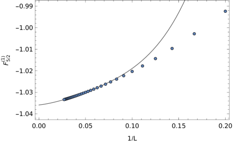
Figure 2: Anomalous dimension of the $q=5/2$ monopole $\Delta_{5/2}^{(1)}$ (4.24, 4.27) as a function of the relativistic cutoff $L$ (4.60) in (a) $\operatorname{QED_{3}}$ ; (b) $\operatorname{QED_{3}-GN}$. The points are obtained by numerically computing Eqs. (4.24, 4.27) and the solid line is a quartic fit in $1/L$ with the points $L\in[L_{\max}-6,L_{\max}]$, here $[31,37]$.

As before, the uncertainty in the scaling dimension is estimated by varying $L_{\max}$ and estimating the anomalous dimension as $L_{\max}\to\infty$. More details are shown in App. I . The resulting scaling dimensions up to $q=7/2$ obtained in this way are shown in Tab. 1. Comparing the $\operatorname{QED_{3}}$ monopoles’ anomalous dimensions with the results in Ref. [61], discrepancies of order $10^{-4}$ to $10^{-3}$ are again observed for higher charges.

Table 1: Leading-order and next-to-leading order in $1/N$ contributions to monopole scaling dimensions in $\operatorname{QED_{3}}$, $\operatorname{QED_{3}-GN}$, and $\operatorname{QED_{3}-Z_{2}GN}$ models. The latter model is discussed in Sec. VII. The leading-order result is the same in all models. The scaling dimension in a given model is $\Delta_{q}=2N\Delta_{q}^{(0)}+\Delta_{q}^{(1)}+O\left(N^{-1}\right)$.

$q$	$\Delta_{q}^{(0)}$	$\Delta_{q,\operatorname{QED_{3}}}^{(1)}$	$\Delta_{q,\operatorname{QED_{3}-GN}}^{(1)}$	$\Delta_{q,\operatorname{QED_{3}-Z_{2}GN}}^{(1)}$
$1/2$	$0.26510$	$-0.038138(5)$	$0.118911(7)$	$0.102846(9)$
$1$	$0.67315$	$-0.19340(3)$	$0.23561(4)$	$0.18663(4)$
$3/2$	$1.18643$	$-0.42109(4)$	$0.35808(6)$	$0.26528(7)$
$2$	$1.78690$	$-0.70482(9)$	$0.4879(2)$	$0.3426(2)$
$5/2$	$2.46345$	$-1.0358(2)$	$0.6254(2)$	$0.4202(3)$
$3$	$3.20837$	$-1.4082(2)$	$0.7705(3)$	$0.4989(3)$
$7/2$	$4.01591$	$-1.8181(2)$	$0.9229(3)$	$0.5789(4)$

The $q=1/2$ results obtained in Sec. IV.2.2 are successfully reproduced with the more general method. Monopole scaling dimensions up to $q=13$ are shown in App. J.

The next-to-leading order term in $1/N$ decreases the scaling dimension of monopoles in $\operatorname{QED_{3}}$ whereas it increases for $\operatorname{QED_{3}-GN}$. That is, quantum corrections help to stabilize the $\operatorname{QED_{3}-GN}$ model and destabilize $\operatorname{QED_{3}}$. To understand the difference between both cases, it is useful to write the scaling dimension as

$$\Delta_{q,\operatorname{QED_{3}-GN}}^{(1)} =\Delta_{q,\operatorname{QED_{3}}}^{(1)}+\Delta_{q,\operatorname{GN}}^{(1)}+\frac{1}{2}\int_{\omega}\sum_{\ell=1}^{\infty}\left(2\ell+1\right)$$

$$\quad{}\times\ln\left[1+\dfrac{\left(1+\frac{\omega^{2}}{\ell(\ell+1)}\right)\left|H_{\ell}^{q,T}(\omega)\right|{}^{2}}{D_{\ell}^{q}(\omega)K_{\ell}^{q,E}(\omega)}\right],$$ (4.70)

where $\Delta_{q,\operatorname{GN}}^{(1)}=\frac{1}{2}\int_{\omega}\sum_{\ell=0}^{\infty}\left(2\ell+1\right)\log\left[D_{\ell}^{q}(\omega)/D_{\ell}^{0}(\omega)\right]$ is the contribution in the $\operatorname{QED_{3}-GN}$ anomalous dimension (4.24) coming exclusively from the pseudo-scalar field. Computing $\Delta_{q,\operatorname{GN}}^{(1)}$ in the same way as we did for $\Delta_{q,\text{$\operatorname{QED_{3}-GN}$}}^{(1)}$ and $\Delta_{q,\operatorname{QED_{3}}}^{(1)}$, we found this contribution is positive $\Delta_{q,\operatorname{GN}}^{(1)}>0$ and more important than the contribution coming exclusively from gauge fields $\big{|}\Delta_{q,\operatorname{GN}}^{(1)}\big{|}>\big{|}\Delta_{q,\operatorname{QED_{3}}}^{(1)}\big{|}$. As for the remaining scalar-gauge contribution in the second line of Eq. (4.70), it is also positive. To see this, we must show that the second term in the logarithm is positive. The numerator is explicitly positive. As for the denominator, we note that $\Delta_{q,\operatorname{GN}}^{(1)}$ is real, meaning that $D_{\ell}^{q}(\omega)$ and the $D_{\ell}^{0}(\omega)$ must have the same sign. The latter $q=0$ kernel is positive, as seen from Eqs.(4.41, 4.44), meaning that $D_{\ell}^{q}(\omega)>0$. The same goes for $K_{\ell}^{q,E}(\omega)$, thus the denominator is positive $D_{\ell}^{q}(\omega)K_{\ell}^{q,E}(\omega)>0$. This does not come as a surprise as these kernels are diagonal entries in the Hessian matrix developed around a minimum saddle-point. The scalar-gauge kernel thus gives a positive contribution to the anomalous dimension in $\operatorname{QED_{3}-GN}$. It then must be that the $\operatorname{QED_{3}-GN}$ monopole anomalous dimension is positive, $\Delta_{q,\operatorname{QED_{3}-GN}}^{(1)}>0$, given what is known about each contribution on the RHS of Eq. (4.70). It would be desirable to understand heuristically why quantum fluctuations render monopoles less relevant at the QCP compared to deep in the Dirac spin liquid.

In the $\operatorname{CP}^{N-1}$ model, similar relations between the different contributions to the monopole anomalous dimension are found. A positive contribution coming only from the auxiliary boson was found numerically in Ref. [62]; the correction from the mixed scalar-gauge kernel can be deduced as positive [63; 64], and the total anomalous dimension of monopoles in $\operatorname{CP}^{N-1}$ numerically found in Ref. [64] is also positive.

IV.2.4 Convexity conjecture

It was recently conjectured that CFT operators charged under a global $\operatorname{U}(1)$ symmetry respect the following convexity relation

$$\Delta((n_{1}+n_{2})n_{0})\geq\Delta(n_{1}n_{0})+\Delta(n_{2}n_{0}),$$ (4.71)

for some positive integer $n_{0}$ of order 1 [65]. We test this conjecture using the monopole operators that are charged under U(1)_top. Here, $n_{0},n_{1},n_{2}$ are integers, where in our notation $\Delta(2q)\equiv\Delta_{q}$. Using the scaling dimensions we obtained in Tab. 5 and extrapolating to finite $N$, we find this relation is respected for the monopoles under consideration in $\operatorname{QED_{3}}$, $\operatorname{QED_{3}-GN}$ (and also for the case $\operatorname{QED_{3}-Z_{2}GN}$ presented later on) for any $2N\in\mathbb{Z}_{+}$ starting from $n_{0}=1$, i.e. the minimal possible value.

V Large-charge universality

In CFTs with a global U(1) symmetry, the related charge $q$ can be used as an expansion parameter by using effective-field-theory methods. It was shown that the lowest scaling dimension among charge-$q$ operators has the following expansion at $q\gg 1$ [54]:

$$\Delta_{q}=c_{3/2}q^{3/2}+c_{1/2}q^{1/2}+\gamma_{\operatorname{U}(1)}+\dots,$$ (5.1)

where the ellipsis denotes negative half-integer and integer powers of $q$ [66]. While $c_{3/2}$ and $c_{1/2}$ depend on the specific $\operatorname{QFT}$ considered, the $O\left(q^{0}\right)$ coefficient is universal (theory independent) [54; 67]:

$$\gamma_{\operatorname{U}(1)}=-0.0937\dots$$ (5.2)

This coefficient is obtained by computing the Casimir energy of the $\operatorname{U}(1)$ Goldstone mode. The Goldstone appears in the state-operator correspondence where the charged operator insertion is mapped to a state where the saddle-point configuration breaks the $\operatorname{U}(1)$ symmetry.

This analysis applies to monopole operators in theories with the global $\operatorname{U}_{\text{top}}(1)$ symmetry group. Given the universality of the coefficient $\gamma$, no term at $O\left(q^{0}\right)$ should be present at leading-order in the $1/N$ expansion, since the leading-order term is proportional to $N$ and thus non-universal. This was indeed observed in $\operatorname{QED_{3}}$, and $\operatorname{O}(2)$- and $\operatorname{O}(3)$-$\operatorname{QED_{3}-GN}$ models [31; 33] as well as in the $\operatorname{CP}^{N-1}$ model [63; 68]. Since $\operatorname{QED_{3}}$ and $\operatorname{QED_{3}-GN}$ monopoles have the same leading-order scaling dimensions, as discussed in Sec. III, this also applies to $\operatorname{QED_{3}-GN}$ monopoles.

Using the monopole anomalous dimensions $\Delta_{q}^{(1)}$, the $O\left(q^{0}\right)$ coefficient $\gamma$ can be computed. This was done for the $\operatorname{CP}^{N-1}$ model in Ref. [68], where $\Delta_{q}^{(1)}$ was obtained for a hundred charges $q=1/2,1,\dots,50$ and the expected expansion (5.1) is fitted numerically to extract $\gamma$. A similar computation is performed here for monopoles in the $\operatorname{QED_{3}-GN}$ and $\operatorname{QED_{3}}$ models. We fit all monopole anomalous dimensions in $\operatorname{QED_{3}-GN}$ and $\operatorname{QED_{3}}$ shown in Tab. 5 by using the fitting function in Eq. (5.1) with powers down to $q^{-1}$ [66]. The fits and the anomalous dimensions are shown in Fig. 3; note that the errors in the values of the anomalous dimension are smaller than the dots in the figure. Including more powers in the fitting function would yield significantly larger errors in the estimation of $\gamma$.

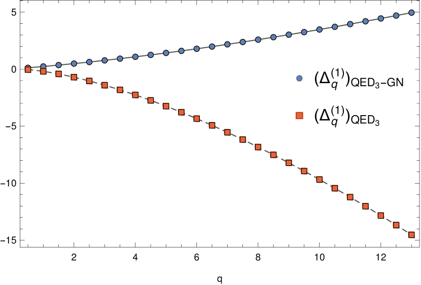
Figure 3: Anomalous dimensions of monopoles in $\operatorname{QED_{3}-GN}$ and $\operatorname{QED_{3}}$ fitted with the large-$q$ expansion (5.1). The points are the scaling dimension corrections obtained with a quartic fit in $1/L$. The solid and dashed lines are the fitting functions for $\operatorname{QED_{3}-GN}$ and $\operatorname{QED_{3}}$, respectively, with a minimal power of $q^{-1}$.

The value of $\gamma$ obtained for each theory is consistent with the expected universal value (5.2)

$$\gamma_{\operatorname{QED_{3}}} =1.02(4)\times\gamma_{\operatorname{U}(1)},$$ (5.3)

$$\gamma_{\operatorname{QED_{3}-GN}} =1.01(6)\times\gamma_{\operatorname{U}(1)}.$$ (5.4)

This is a nice consistency check of the anomalous scaling dimensions obtained in the last section.

The universal coefficient of the scaling dimension of $\operatorname{U}(1)$-charged operators in Eq. (5.1) can also be formulated with the following sum rule [54]

$$q^{2}\Delta_{q}-\left(\frac{q^{2}}{2}+\frac{q}{4}+\frac{3}{16}\right)\Delta_{q-1}-\left(\frac{q^{2}}{2}-\frac{q}{4}+\frac{3}{16}\right)\Delta_{q+1}$$

$$=-\frac{3}{8}\gamma_{\operatorname{U}(1)}+O\bigl{(}q^{-1/2}\bigr{)}=0.0351\dots$$ (5.5)

The RHS results from a cancellation of order $O\left(q^{3/2}\right)$ and $O\left(q^{1/2}\right)$ terms on the LHS. In comparison, the error on the LHS coming from the triplet $\Delta_{q-1},\Delta_{q},\Delta_{q+1}$ is comparatively large, even more so as the coefficients in front of the scaling dimensions, which are of order $q^{2}$, become larger with increasing $q$. The resulting errors are too important to obtain a reliable fit of the large-$q$ behaviour of this sum rule. Nevertheless, we did observe a good qualitative agreement for the scaling dimensions shown in Tab. 5.

VI CFT duality: $\operatorname{QED_{3}-GN}$ and $\operatorname{CP}^{1}$ models

Another interesting application of our results concerns the duality between the $\operatorname{QED_{3}-GN}$ model with $2N=2$ two-component Dirac fermion flavors and the $\operatorname{CP}^{N-1}$ model with $N=2$ complex boson flavors [53]. Crucially, the duality between these models implies an emergent $\operatorname{SO}(5)$ symmetry. The following $\operatorname{SO}(5)$ multiplet in the $\operatorname{QED_{3}-GN}|_{2N=2}$ model

$$\begin{split}\bigg{(}&\real(\psi_{1}^{\dagger}\widetilde{\mathcal{M}}_{1/2}^{f}),-\imaginary(\psi_{1}^{\dagger}\widetilde{\mathcal{M}}_{1/2}^{f}\bigr{)},\\ &\real(\psi_{2}^{\dagger}\widetilde{\mathcal{M}}_{1/2}^{f}),\imaginary(\psi_{2}^{\dagger}\widetilde{\mathcal{M}}_{1/2}^{f}),\phi\bigg{)},\end{split}$$ (6.1)

is dual to the following multiplet in the $\operatorname{CP}^{1}$ model

$$\left(2\real(\mathcal{M}_{1/2}^{b}),2\imaginary(\mathcal{M}_{1/2}^{b}),z^{\dagger}\sigma_{1}z,z^{\dagger}\sigma_{2}z,z^{\dagger}\sigma_{3}z\right).$$ (6.2)

Here $\widetilde{\mathcal{M}}_{1/2}^{f}$ are the $\operatorname{QED_{3}-GN}|_{2N=2}$ minimally charged monopoles which must be dressed with an additional zero mode $\psi_{1}^{\dagger}$ or $\psi_{2}^{\dagger}$ on top of a Dirac sea in order to be gauge invariant. These monopoles form an $\operatorname{SU}(2$) doublet $\mathcal{M}_{1/2}^{f}=\left(\mathcal{M}_{1/2,\uparrow}^{f},\mathcal{M}_{1/2,\downarrow}^{f}\right)^{\intercal}$. On the $\operatorname{CP}^{1}$ side, $z$ is an $\operatorname{SU}(2)$ doublet $z=\left(z_{1},z_{2}\right)^{\intercal}$ where each flavor is a complex boson and $\mathcal{M}_{1/2}^{b}$ is the minimally charged monopole. The $\operatorname{SO}(5)$ symmetry means that all scaling dimensions within a multiplet should be equal, while operators identified by the duality should also have the same scaling dimension. Putting this together, this means that all the operators above should have the same scaling dimension. A decent agreement was already observed in Ref. [31], but the scaling dimension of $\operatorname{QED_{3}-GN}$ monopoles were obtained only at leading-order in $1/N$, with $\Delta_{\mathcal{M}_{1/2}^{f}}=0.53$. Updating the comparison with the next-to-leading order correction, we find $\Delta_{\mathcal{M}_{1/2}^{f}}=0.65,$ which gives an even better agreement. For instance, the scaling dimension of the $q=1/2$ monopole on the $\operatorname{CP}^{1}$ side obtained at next-to-leading in $1/N$ is given by $\Delta_{\mathcal{M}_{1/2}^{b}}=0.63$ [63; 64]. In contrast, if we extrapolate the large-$N$ QED₃ result to $2N=2$, we obtain a scaling dimension of 0.49, which is further from the $\operatorname{CP}^{1}$ result, as expected since the two CFTs are not related by duality. The scaling dimensions of the other operators in the duality also show a good agreement coming from both analytical and numerical studies, as shown in Tab. 2.

Table 2: Operators in the $\operatorname{SO}(5)$ $\boldsymbol{5}$ multiplets (6.1, 6.2) and their scaling dimensions. “VBS” and “Néel” make reference to operators whose scaling dimensions are obtained numerically on lattices. The results for monopole operators are obtained by using the state-operator correspondence at next-to-leading order in $1/N$. The scaling dimension of the auxiliary boson $\phi$ in $\operatorname{QED_{3}-GN}$ was obtained at order $1/N$ using the mean of Padé and Padé-Borel $[0/1]$ resummations (non-resummed scaling dimension are unphysical). The scaling dimension of the fermionic monopole operator can also be resummed to $(0.59,0.68)$, but not in the bosonic case. The operator $z^{\dagger}\bm{\sigma}z$ designates any of the boson bilinears, i.e. flavor spin-1 in the bosonic side. It was obtained at order $1/N^{2}$ in Ref. [69] and using functional renormalization group in Ref. [70].

$\mathcal{O}$	$\Delta_{\mathcal{O}}$	Ref.
$\mathcal{M}_{1/2}^{f}$	$0.65$	This work
$\mathcal{M}_{1/2}^{b}$	$0.63$	[64]
$\phi$	$(0.59,0.64)$	[47]
$z^{\dagger}\bm{\sigma}z$	$0.64$	[69]
	$0.61$	[70]
VBS, Néel	$[0.60,0.68]$	[71; 72; 73; 74; 75]

In the same way, monopoles with the second smallest charge $q=1$ were argued to be part of the symmetric traceless $\boldsymbol{14}$ representation of $\operatorname{SO}(5)$ [44; 69]. The various relevant scaling dimensions obtained with analytical methods are also compared in Tab. 3. Again there is a very good agreement between the scaling dimension of monopole operators, with $\Delta_{\mathcal{M}_{1}^{f}}=1.58$ and $\Delta_{\mathcal{M}_{1}^{b}}=1.50$. The agreement is weaker with other operators, but by taking into account Padé and Padé-Borel resummations the duality prediction seems quite reasonable. The scaling dimension related to auxiliary bosons $\Delta_{\phi^{2}}$ and $\Delta_{\lambda}$ obtained using the large-$N$ have greater discrepancy with $\Delta\sim 1$, but these expansions are not very well controlled. However, the same can be said about the monopole operator on the bosonic side. Overall, the duality for the $\boldsymbol{14}$ representation of $\operatorname{SO}(5)$ is not as convincing as for the $\boldsymbol{5}$, but still reasonable for perturbative results. The scaling dimension of the Lagrange field obtained using the functional renormalization group also agrees reasonably well $\Delta_{\lambda}=1.21$ [70].

Table 3: Operators in the $\operatorname{SO}(5)$ symmetric traceless $\boldsymbol{14}$ multiplets and their scaling dimensions predicted to be equal according to the duality between $\operatorname{QED_{3}-GN}|_{2N=2}$ and $\operatorname{CP}^{1}$ models. The scaling dimensions presented are obtained analytically with the large-$N$ expansion. Padé and Padé-Borel $[0/1]$ resummations are shown in parenthesis (apart from Ref. [47], resummations are not obtained in the references cited). The symbol “$\times$” indicates unphysical results, i.e., negative scaling dimensions. The operator $\lambda$ is the Lagrange multiplier field on the $\operatorname{CP}^{1}$ side. Results for monopole operators are obtained using state-operator correspondence at order $N^{0},$ while other results were obtained at order $N^{-1}$. The resummed value for $\Delta_{\bar{\psi}\bm{\sigma}\psi}$ was obtained in Ref. [47] and is the same for $\Delta_{(z^{*}\bm{\sigma}z)(z^{*}\bm{\sigma}z)^{\intercal}}$ at this order.

$\mathcal{O}$	$\Delta_{\mathcal{O}}$	$(\Delta_{\mathcal{O}}^{\text{Pad\'{e}}},\Delta_{\mathcal{O}}^{\text{Pad\'{e}-Borel}})$	Ref.
$\mathcal{M}_{1}^{f}$	$1.58$	$(1.63,1.75)$	This work
$\mathcal{M}_{1}^{b}$	$1.50$	$(\times,0.24)$	[64]
$\bar{\psi}\bm{\sigma}\psi$	$1.19$	$(1.42,1.51)$	[47; 69]
$\left(z^{\dagger}\bm{\sigma}z\right)\left(z^{\dagger}\bm{\sigma}z\right)^{\intercal}$	$1.19$	$(1.42,1.51)$	[69]
$\phi^{2}$	$4.43$	$(\times,1.02)$	[47; 69]
$\lambda$	$\times$	$(0.90,1.11)$	[76; 77]

The situation becomes more puzzling when the critical exponents in Tab. 3 are compared to numerical lattice results. The apparent consistency observed in the analytical results (at least for operators that do not need resummation) does not hold for the numerical lattice results. Specifically, we compare the analytical results to the correlation length exponent $\nu$ obtained in many numerical studies of the $\operatorname{CP}^{1}$ model. This exponent is related to the Lagrange field scaling dimension as $\Delta_{\lambda}=3-1/\nu$. Its value has varied greatly among many numerical works. Earlier results indicate that $\Delta_{\mathcal{\lambda}}\in[1.34,1.67]$ [71; 72; 78; 79] which seems compatible with other scaling dimensions in Tab. 3. However, unusual scaling behaviour and the “drifting” of $\nu$ with increasing lattice size [75] motivated further studies, and lower scaling dimensions have been found. The wide range of values obtained are shown in Tab. 4. Notably, a scaling dimension going down to $\Delta_{\lambda}=0.80(1)$ by considering the presence of a second length scale [80].

The varying results among different lattice studies were also interpreted as a hint for a weakly first-order transition. This possibility has been discussed [69; 81] in a field theory context where the dual models $\operatorname{QED_{3}-GN}|_{2N=2}$ and $\operatorname{CP}^{N-1}|_{N=2}$ are possibly complex $\operatorname{CFT}$s emerging from the collision of fixed points as the number of matter flavors is lowered below a critical level. On the other hand, our analytical analysis shows there is still consistency among scaling dimensions on both sides of the duality. This may imply that the duality can still give valuable information, even if the CFT is non-unitary.

Table 4: Numerical determination of the correlation length exponent $\nu$ and the related scaling dimension $\Delta_{\lambda}=3-1/\nu$ in lattice studies describing the $\operatorname{CP}^{1}$ side.

$\nu$	$\Delta_{\mathcal{\lambda}}$	Ref.
$0.78(3)$	$1.72(5)$	[71]
$0.68(4)$	$1.52(9)$	[72]
$\biggl{\{}\!\!$ $0.67(1)$ $0.69(2)$ $\biggl{\{}\!\!$	$1.51(3)$ $1.55(5)$	[79]
$0.62(2)$	$1.39(5)$	[78]
$0.54(5)$	$1.13(17)$	[74]
$[0.51,0.69]$	$[1.04,1.55]$	[82]
$0.468(6)$	$0.87(3)$	[75]
$0.455(2)$	$0.80(1)$	[80]

A similar tension between the results from field theory and lattice models was observed in Ref. [83] where the $\operatorname{QED_{3}}|_{2N=2}$ model was studied using conformal bootstrap. The duality to the easy-plane $\operatorname{CP}^{1}$ model conjectured in Ref. [53] implies a self-duality and an emergent $\operatorname{O}(4)$ symmetry on both sides. While the conformal bootstrap study of $\operatorname{QED_{3}}|_{2N=2}$ is consistent with the self-duality and the emergent symmetry, it contradicts results from the lattice study of the easy-plane $\operatorname{CP}^{1}$ model [84].

An interesting approach to understand these discrepancies could be that of pseudo-criticality, that is a weakly first-order transition with a generically long correlation length. In Ref. [85], a Wess-Zumino-Witten model in $2+\epsilon$ dimensions, with target space $S^{3+\epsilon}$, with global symmetry $\operatorname{SO}(4+\epsilon)$ has been shown to exhibit this behaviour and consistent with numerical results in the literature. A crucial point was that the physical dimension $d=3$ is close to the critical dimension $d=2.77$ where fixed points collide. Pseudo-criticality was also found in a loop model describing the easy-plane Néel-VBS transition [86].

Higher charge

The duality can be tested further by comparing monopoles on both sides of the duality. First, the relation between minimally charged monopoles is further discussed. This relation is simpler to see with the appropriate sub-models. A duality between $\operatorname{QED_{3}}|_{2N=2}$ and easy-plane $\operatorname{CP}^{1}$ was formulated by including additional external gauge fields $B_{\mu},B_{\mu}^{\prime}$ and Chern-Simons terms [87; 53]

$$\left|D_{b+B}z_{1}\right|^{2}+\left|D_{b+B^{\prime}}z_{2}\right|^{2}-\left|z_{1}\right|^{4}-\left|z_{2}\right|^{4}$$

$$\quad{}-\frac{1}{2\pi}bd\left(B+B^{\prime}\right)-\frac{1}{2\pi}BdB^{\prime}-\frac{1}{2\pi}B^{\prime}dB$$ (6.3)

$$\Leftrightarrow\quad \overline{\psi}_{1}i\not{D}_{a-B}\psi_{1}+\overline{\psi}_{2}i\not{D}_{a+B}\psi_{2}+\frac{1}{2\pi}adB^{\prime}$$

$$\quad{}+\frac{1}{4\pi}\left(BdB-B^{\prime}dB^{\prime}\right),$$ (6.4)

where $b_{\mu}$ and $a_{\mu}$ are the dynamical gauge fields in bosonic and fermionic models, respectively. By inspecting the charges under the external gauge fields $\left(q_{B},q_{B^{\prime}}\right)$, we can identify the following bosonic operators

$$(2\mathcal{M}_{1/2}^{b},2z_{1}^{*}z_{2})\Leftrightarrow\left((\psi_{1}^{\dagger}\widetilde{\mathcal{M}}_{1/2}^{f})^{\dagger},\psi_{2}^{\dagger}\widetilde{\mathcal{M}}_{1/2}^{f}\right).$$ (6.5)

Here, the first and second component on both sides have charges $(1,1)$ and $(1,-1)$ under $B_{\mu}$ and $B^{\prime}_{\mu}$. While an $\operatorname{SU}(2)$ doublet structure is manifest in the RHS with the fermion zero modes, it is less clear in the LHS and may be seen as a non-trivial corollary of the duality. This may however be motivated by the self-duality in the easy-plane $\operatorname{CP}^{1}$ model. The VBS order in the original model $\mathcal{M}_{1/2}^{b}$ is mapped to the XY order in terms of the dual bosons $w_{1}^{*}w_{2}$. Conversely, monopoles in the dual side are mapped to $z_{1}^{*}z_{2}$ in the original model.

These relations between operators translate back to the $\operatorname{QED_{3}-GN}|_{2N=2}\Leftrightarrow\operatorname{CP}^{1}$ duality. In particular, it is useful to focus on the dual relation between the $\operatorname{CP}^{1}$ monopole $2\mathcal{M}_{1/2}^{f}$ and the corresponding dual monopole in $\operatorname{QED_{3}-GN}|_{2N=2}$, $\bigl{(}\psi_{1}^{\dagger}\widetilde{\mathcal{M}}_{1/2}^{f}\bigr{)}^{\dagger}$. For convenience, we define the following monopole operator $\mathcal{M}_{1/2}^{f}(x)\equiv 2\bigl{(}\psi_{1}^{\dagger}\widetilde{\mathcal{M}}_{1/2}^{f}\bigr{)}^{\dagger}$. Our starting point is then the conjectured dual relation between minimally charged monopoles in $\operatorname{QED_{3}-GN}|_{2N=2}$ $(\mathcal{M}_{1/2}^{f})$ and in $\operatorname{CP}^{1}$ $(\mathcal{M}_{1/2}^{b})$ models

$$\mathcal{M}_{1/2}^{f}(x)\Leftrightarrow\mathcal{M}_{1/2}^{b}(x).$$ (6.6)

Using this relation and the operator product expansion ($\operatorname{OPE}$)

$$\mathcal{O}_{1}(x)\mathcal{O}_{2}(y)=\sum_{n}c_{n}(x-y)\mathcal{O}_{n}(y),$$ (6.7)

the scaling dimensions of higher charge monopoles can also be compared. The $\operatorname{OPE}$ of two $q=1/2$ monopole operators yields the expansion over $q=1$ operators

$$\lim_{y\to x}\mathcal{M}_{1/2}(x)\mathcal{M}_{1/2}(y) =\lim_{y\to x}c(x-y)\mathcal{M}_{1}(x)+\cdots$$ (6.8)

where the ellipsis stands for other primary operators with larger scaling dimensions. By definition, $\mathcal{M}_{1}(x)$ has the smallest scaling dimension in the $q=1$ topological sector. We can then identify the scaling dimension of $q=1$ monopole operators on both sides of the duality $\Delta_{q=1}^{f}=\Delta_{q=1}^{b}.$ This is expected, as these monopoles are conjectured to be components dual $\operatorname{SO}(5)$ symmetric traceless $\boldsymbol{14}$ multiplet [44; 69]. Using the same logic for higher charge monopoles, we find more generally that

$$\Delta_{q}^{f}=\Delta_{q}^{b}.$$ (6.9)

Comparing our results for $\operatorname{QED_{3}-GN}|_{2N=2}$ monopoles in Tab. 1 to $\operatorname{CP}^{1}$ monopoles in Ref. [68], we obtain a good agreement for higher charges, as shown in Fig. 4. For larger charges, the relative difference tends to $10\%$. This is a great improvement compared to the results obtained with only the leading-order scaling dimensions: the behaviour is similar and the asymptotic relative difference for large $q$ is $76\%$ instead.

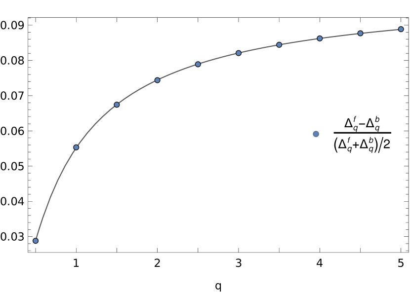
Figure 4: Relative difference between the scaling dimensions of monopoles in $\operatorname{QED_{3}-GN}|_{2N=2}$ and $\operatorname{CP}^{1}$ models as a function of the topological charge. The computation is done with next-to-leading-order results in both models. The solid line is a fit $f_{0}+f_{-1}q^{-1}+f_{-3/2}q^{-3/2}$, where the asymptote for large charge is approximately a $10\%$ relative difference. The powers used in the fitting function are deduced from Eq. (5.1).

VII Transition to $Z_{2}$ spin liquids

In this section, we consider quantum critical transitions to $Z_{2}$ spin liquids. The pairing of the spinons gaps out the gauge field through the Higgs mecanism. We begin with the most symmetric pairing interaction, and we then discuss the more general case where the pairing further breaks the flavor symmetry.

VII.1 Symmetric $Z_{2}$ spin liquid

The transition out of the U(1) DSL to a $Z_{2}$ spin liquid can also be studied with a gauged Gross-Neveu model [51; 30; 49; 50]. The Lagrangian describing this transition is written in euclidean flat spacetime as

$$\mathcal{L}_{\psi} =\sum_{i=1}^{2N}-\overline{\psi}_{i}(\not{\partial}-i\not{\mathcal{A}}_{q}-i\not{A})\psi_{i}$$

$$\quad+\sum_{i=1}^{2N}(\phi^{*}\psi_{i}^{T}i\gamma_{2}\psi_{i}+\text{h}.\text{c}.),$$ (7.1)

where $\phi$ is a complex scalar that decouples a quartic superconducting pairing term for the fermions. The interaction term included preserves Lorentz invariance. As $\phi$ describes Cooper pairs, it transforms as $\bar{\psi}_{i}i\gamma_{2}\bar{\psi}_{i}^{T}$ under U(1) gauge transformations. The Yukawa interaction term in the above equation is thus gauge invariant. In the $Z_{2}$ QSL, $\phi$ acquires an expectation value, which Higgses the gauge field, leading to a gapped $s$-wave superconducting state for the Dirac fermions.

We recall that the Dirac conjugate is defined by $\overline{\psi}_{i}=\psi_{i}^{\dagger}\gamma_{0}$ and $\mathcal{A}^{q}_{\mu}$ is the external gauge field that sources the flux of $4\pi q$. The gauge-covariant derivative for the external gauge field $\mathcal{A}_{\mu}^{q}$ on a curved spacetime is defined in Eq. (2.13). We now introduce the Nambu spinor defined as

$$\Upsilon_{i}=\left(\begin{array}[]{c}\psi_{i}\\ i\gamma_{2}\overline{\psi}_{i}^{T}\end{array}\right)=\left(\begin{array}[]{c}\psi_{i}\\ C\overline{\psi}_{i}^{T}\end{array}\right).$$ (7.2)

In addition, we define $\mathcal{C}=\text{diag}(C,C)$, where $C=i\gamma_{2}$. The $C$ operator obeys $C^{2}=-1$, $C^{T}=C^{-1}=-C$, and $C\gamma_{\mu}C=\gamma_{\mu}^{T}$. The transpose of the Nambu spinor is given by $\Upsilon_{i}^{T}=(\psi_{i}^{T},\overline{\psi}_{i}C^{T})=(\psi_{i}^{T},-\overline{\psi}_{i}C)$. Thus, the fermionic action can be expressed as

$$S_{\Upsilon}=\frac{1}{2}\int_{r,r^{\prime}}\Upsilon_{i}^{T}(r)\mathcal{C}\mathcal{G}^{-1}(r,r^{\prime})\Upsilon_{i}(r^{\prime}),$$ (7.3)

where the (inverse) Nambu Green’s function is

$$\mathcal{G}^{-1}(r,r^{\prime})=\begin{pmatrix}2\phi^{*}(r)&-\not{D}_{-(A+\mathcal{A}_{q})}\\ -\not{D}_{A+\mathcal{A}_{q}}&2\phi(r)\end{pmatrix}\delta(r-r^{\prime}).$$ (7.4)

As in Sec. IV, the fields $\phi$ and $A$ are expanded about their saddle-point values as $\phi=\left\langle\phi\right\rangle+\sigma/\sqrt{2N}$, $A=\left\langle A\right\rangle+a/\sqrt{2N}$, where the fluctuations are suppressed by $1/\sqrt{2N}$. At the QCP, the saddle-point values are $\left\langle\phi\right\rangle=\left\langle A\right\rangle=0$ [50]. Thus, in terms of the saddle-point and fluctuation fields, the inverse Green’s function is

$$\mathcal{G}^{-1}(r,r^{\prime}) =\mathcal{G}_{0}^{-1}(r,r^{\prime})+\frac{1}{\sqrt{2N}}X_{\sigma}(r)\delta(r-r^{\prime})$$

$$\quad+\frac{1}{\sqrt{2N}}X_{a}(r)\delta(r-r^{\prime}).$$ (7.5)

Here, $\mathcal{G}^{-1}_{0}$ is the bare inverse Green’s function, determined from the gauge covariant derivative term involving $\mathcal{A}^{q}_{\mu}$ in Eq. (7.4), and $X_{\sigma}$ and $X_{a}$ are given by

$$X_{\sigma}=2\begin{pmatrix}\sigma^{*}&0\\ 0&\sigma\end{pmatrix},\quad X_{a}=\begin{pmatrix}0&-\not{a}\\ \not{a}&0\end{pmatrix}.$$ (7.6)

Integrating out the fermions then gives the effective action as $\int\mathcal{D}\Upsilon\exp(-S_{\Upsilon})\equiv\exp(-S_{\operatorname{eff}}),$ where $S_{\operatorname{eff}}=-\frac{1}{2}(2N)\text{Tr}\log\mathcal{G}^{-1}$. We let Tr denote a “trace” over all relevant degrees of freedom, whereas tr denotes a trace over spinor components. To compute the effective action, we express the fermionic action as a quadratic form in the fluctuation fields and perform a Gaussian functional integral over $a$ and $\sigma$. The linear terms in $a$ and $\sigma$ vanish due to the saddle-point conditions for $A$ and $\phi$. Thus, to quadratic order, the effective action becomes

$$S_{\operatorname{eff}} =\left.S_{\operatorname{eff}}\right|_{\text{s.p.}}+\frac{1}{4}\text{Tr}\,\mathcal{G}_{0}X_{a}\mathcal{G}_{0}X_{a}+\frac{1}{4}\text{Tr}\,\mathcal{G}_{0}X_{a}\mathcal{G}_{0}X_{\sigma}$$

$$\quad+\frac{1}{4}\text{Tr}\,\mathcal{G}_{0}X_{\sigma}\mathcal{G}_{0}X_{a}+\frac{1}{4}\text{Tr}\,\mathcal{G}_{0}X_{\sigma}\mathcal{G}_{0}X_{\sigma}.$$ (7.7)

The fluctuations are $O(1/(2N))$, thus they cancel the prefactor $2N$. The second and third terms involve both the gauge field and the scalar field. By taking the trace over the Nambu matrix structure, these terms are found to vanish. Indeed, these terms must vanish from gauge invariance. Hence, only the gauge-gauge and scalar-scalar kernels contribute, which is in contrast to the QED₃-GN case where mixing between the two sectors exists. After performing the trace over the Nambu indices, the scalar-scalar kernel is

$$\frac{1}{4}\text{Tr}\,\mathcal{G}_{0}(r^{\prime},r)X_{\sigma}(r)\mathcal{G}_{0}(r,r^{\prime})X_{\sigma}(r^{\prime})$$

$$=\int_{r,r^{\prime}}\sigma^{*}(r)D(r,r^{\prime})\sigma(r^{\prime}),$$ (7.8)

where the scalar kernel is the same as in Eq. (4.9). Similarly, the gauge-gauge kernel is the same as in QED₃:

$$\frac{1}{4}\text{Tr}\,\mathcal{G}_{0}(r^{\prime},r)X_{a}(r)\mathcal{G}_{0}(r,r^{\prime})X_{a}(r^{\prime})$$

$$=\frac{1}{2}\int_{r,r^{\prime}}a_{\mu}(r)K_{\mu\nu}(r,r^{\prime})a_{\nu}(r^{\prime}),$$ (7.9)

where the gauge-gauge kernel is the same as in Eq. (4.10). Combining these two results we find that the fluctuation action (obtained after integrating out $\sigma$ and $a$) is just the sum of twice the pure $\operatorname{GN}$ and the $\operatorname{QED_{3}}$ results. The anomalous dimension for the minimal charge $q=1/2$ is thus deduced to be

$$\Delta_{\operatorname{QED_{3}-Z_{2}GN}}^{(1)}=\Delta_{\operatorname{QED_{3}}}^{(1)}+2\Delta_{\operatorname{GN}}^{(1)}=0.102846(9).$$ (7.10)

The value and the error are estimated in the same way as described in Sec. IV and App. I by finding an expression similar to Eq. (4.24) for the $\operatorname{QED_{3}-Z_{2}GN}$ case. The result is surprisingly close to the $\operatorname{QED_{3}-GN}$ case, although the quantum fluctuations possess a different structure at the two transitions. In Table 1, we give the answer for higher $q$. It can be seen that the values of the anomalous dimensions for $q>1/2$ for the CSL and $Z_{2}$ QSL are not as close as in the case of the minimal charge. By using anomalous dimensions up to $q=13$ shown in App. J, one can again confirm the value of the universal coefficient for CFTs with a $\operatorname{U}(1)$ global symmetry as described in Sec. V: In this case, we find $\gamma_{\operatorname{QED_{3}-Z_{2}GN}}=0.98(7)\times\gamma_{\operatorname{U}(1)}$.

VII.2 More general $Z_{2}$ spin liquids

Let us now consider a more general (superconducting) pairing interaction given by

$$\mathcal{L}_{\mathrm{int}}=\sum_{i=1}^{2N}\phi^{*}_{I}\psi^{T}_{i}CM^{I}_{ij}\psi_{j}+\mathrm{h.c.}.$$ (7.11)

Here, $C$ is the same as in the previous subsection – an antisymmetric and unitary matrix with indices denoting the Dirac indices of the spinor $\psi$. The additional term in the interaction $M^{I}$ represents a “flavor” matrix, which is symmetric and has indices in the valley and spin spaces. We shall consider some simple concrete examples of $M$ later in this section. The index $I$, which is implicitly summed over, corresponds to the number of charged scalar fields, i.e., the competing pairing channels. In the previous section $I=1$ and $M$ corresponds to the identity operator.

The analysis for this more general pairing interaction follows the same lines as before. The Nambu spinor is the same as in Eq. (7.16), however, the inverse Green’s function now becomes

$$\mathcal{G}^{-1}(r,r^{\prime})=\begin{pmatrix}2\phi_{I}^{*}(r)M^{I}&-\not{D}_{-(A+\mathcal{A}_{q})}\\ -\not{D}_{A+\mathcal{A}_{q}}&2\phi_{I}(r)M^{I}\end{pmatrix}\delta(r-r^{\prime}).$$ (7.12)

Here we suppose that $M$ is hermitian. The inverse Green’s function can be expanded again using the large-$N$ formalism, and the effective action can be similarly expressed as in Eq. (VII.1). The terms involving both the gauge field and the scalar field again vanish due to gauge invariance, and the gauge-gauge term is the same as in Eq. (VII.1). The scalar-scalar kernel is now

$$\frac{1}{4}\text{Tr}\mathcal{G}_{0}(r^{\prime},r)X_{\phi}(r)\mathcal{G}_{0}(r,r^{\prime})X_{\phi}(r^{\prime})$$

$$=-\sum_{I,J}\int_{r,r^{\prime}}\phi_{I}^{*}(r)D(r,r^{\prime})\phi_{I}(r^{\prime})\mathrm{tr}((M^{I})^{2})\delta_{IJ}.$$ (7.13)

where we have assumed that the different channels labelled by $I$ are orthogonal: $\mathrm{tr}(M^{I}M^{J})=0$ if $I\neq J$. Then, the anomalous dimension is

$$\Delta_{\operatorname{QED_{3}-Z_{2}GN}^{\prime}}^{(1)}=\Delta_{\operatorname{QED_{3}}}^{(1)}+2\Delta_{\operatorname{GN}}^{(1)}\frac{\sum_{I}\mathrm{tr}[(M^{I})^{2}]}{2N}.$$ (7.14)

In the previous section, $M^{I}$ was the identity operator and so $\mathrm{tr}[(M^{I})^{2}]=2N$, which leads to the previous result for the anomalous dimension in Eq. (7.10). As another example, consider the case where the pairing interaction is of the form $\phi_{x}\psi^{T}C\sigma_{x}\psi+\phi_{z}\psi^{T}C\sigma_{z}\psi$; note that we cannot use $\sigma_{y}$ since it is not symmetric. In this case $\sum_{I}\mathrm{tr}[(M^{I})^{2}]=4N$, and so the anomalous dimension of the second term in Eq. (7.14) is now four times the pure-GN result.

Note that the superconducting pairing generally reduces the flavor (spin/valley) global symmetry. Therefore, monopole operators with different flavor quantum numbers are expected to have different scaling dimensions, resulting in a hierarchy of monopoles [33]. As our present formalism selects only the monopole with the smallest scaling dimension, a constraint on the flavor quantum numbers would be needed to describe other monopoles. Moreover, since the pairing field cannot have an expectation value for gauge invariant monopoles, it is expected that next-to-leading corrections are necessary to observe this hierarchy. Generalizing Ref. [33] to quantify this effect would be an interesting avenue to explore.

To understand these more general $Z_{2}$ spin liquids, we analyze the pairing Hamiltonian in further detail. In particular, here we shall focus on the Bogoliubov-de Gennes (BdG) Hamiltonian for the mean-field description of Eq. (7.11). In the preceding section we formulated the theory in terms of a Euclidean Lagrangian description. Since the Hamiltonian $\mathcal{H}$ is the time-component of an energy momentum tensor, it is necessarily a non-Lorentz-invariant entity. Thus, here we shall use Minkowski spacetime to perform the analysis, which enables standard field theory methods to determine $\mathcal{H}$ from $\mathcal{L}$.

We define $\mathcal{H}=\pi\dot{\psi}-\mathcal{L}$, where $\pi$ is the canonical momentum conjugate to $\psi$. From Eqs. (VII.1) (without the gauge field) and (7.11), we construct the following Hamiltonian

$$\mathcal{H}=-\left(i\psi^{\dagger}_{i}\gamma^{0}\boldsymbol{\gamma}\cdot\boldsymbol{\nabla}\psi_{i}+\phi^{*}_{I}\psi^{T}_{i}CM^{I}_{ij}\psi_{j}+\mathrm{h.c.}\right).$$ (7.15)

Our choice of gamma matrices is given by $\gamma^{\mu}=\left(\tau_{z},i\tau_{x},i\tau_{y}\right)$; this definition is consistent with the Clifford algebra with a mostly minus metric. Here, $C=i\tau_{y}$. We define the Nambu spinor $\chi(k)$ by

$$\chi_{i}(k)=\left(\begin{array}[]{c}\psi_{i}(k)\\ C\psi^{*}_{i}(-k)\end{array}\right).$$ (7.16)

In terms of the Nambu spinor $\chi(k)$, the Hamiltonian has the following form in momentum space:

$$\mathcal{H}=\frac{1}{2}\int_{k}\chi_{i}^{\dagger}\left(k\right)\left(\begin{array}[]{cc}\delta_{ij}\gamma^{0}\bm{\gamma}\cdot\bm{k}&-2\phi_{ij}\\ -2\phi^{*}_{ij}&-\delta_{ij}\gamma^{0}\bm{\gamma}\cdot\bm{k}\end{array}\right)\chi_{j}\left(k\right),$$ (7.17)

where $\phi_{ij}^{*}=\phi_{I}^{*}M_{ij}^{I}$. In general, the Hamiltonian can be expressed as $\mathcal{H}=\frac{1}{2}\int_{k}\chi_{i}^{\dagger}\left(k\right)H(k)\chi_{j}\left(k\right)$, where $H(k)$ is the BdG matrix. In the simplest case we have $2N=2$, that is, there are 2 spin degrees of freedom, and the BdG Hamiltonian is $8\times 8$. In the previous section we considered the case where the pairing matrix is the identity, $M^{I}=\Delta\sigma_{0}$, where $\Delta$ is the finite value of the pairing term in the $Z_{2}$ spin liquid phase.

Here we contemplate some simple examples of pairing matrices, namely $M^{I}=\Delta\sigma_{x}$ or $M^{I}=\Delta\sigma_{z}$. For these classes of spin liquids, the BdG matrix is of the form

$$H(k) =\sigma_{0}\otimes\left(\begin{array}[]{cc}1&0\\ 0&-1\end{array}\right)\otimes\left(-\tau_{y}k_{x}+\tau_{x}k_{y}\right)$$ (7.20)

$$\quad+\sigma_{l}\otimes\left(\begin{array}[]{cc}0&-2\Delta\\ -2\Delta^{*}&0\end{array}\right)\otimes\tau_{0},$$ (7.23)

Here $\sigma_{l}=\sigma_{0},\sigma_{x},$ or $\sigma_{z}$. The various matrices appearing above correspond to the spin indices, Nambu indices, and finally the Dirac indices, respectively. For the simple case where $\sigma_{l}=\sigma_{0}$, the eigenvalues are given by $E(k)=\pm\sqrt{{\bf k}^{2}+4\left|\Delta\right|^{2}},$ with a fourfold degeneracy. These eigenvalues are exactly the same as in the Fu-Kane model at half filling [88]. Indeed, in the Fu-Kane model the Hamiltonian is a $4\times 4$ matrix with spin and Nambu indices. Here we have two copies of this model Hamiltonian for each species of spin. In the case where $\sigma_{l}=\sigma_{x}$ or $\sigma_{z}$, we also have the same dispersion. In general, this dispersion describes a gapped $\mathbb{Z}_{2}$ spin liquid. The QCP in the present model is generally thought to be well defined at modest values of $N$; we can incorporate $N$ copies of the valley degrees of freedom and obtain the same (copies) of the eigenvalues.

For the case where we have two competing channels, $M^{I}=\Delta_{x}\sigma_{x}+\Delta_{z}\sigma_{z}$, the dispersion is given by $E_{\pm,\pm}(k)=\pm\sqrt{{\bf k}^{2}+\left|2\Delta_{x}\right|^{2}+\left|2\Delta_{z}\right|^{2}\pm 4\left|\Delta_{x}\Delta_{z}^{*}-\Delta_{x}^{*}\Delta_{z}\right|}$, with twofold degeneracy. In the case where either $\Delta_{x}$ or $\Delta_{z}$ is equal to zero, we recover the previous result for the eigenvalues. Interestingly, for the specific case where $\left|\Delta_{x}\right|=\left|\Delta_{z}\right|$ and $\mathrm{arg}(\Delta_{x})-\mathrm{arg}(\Delta_{z})=\pm\pi/2$ (mod $\pi$), there are gapless Dirac cones, $\pm k$. For such pairings, we thus have a gapless $Z_{2}$ spin liquid with massless relativistic fermions, and a gapped $Z_{2}$ gauge field.

This last case can be reformulated as a pairing term given by $M^{I}=|\Delta|\vec{d}\cdot\sigma_{y}\vec{\sigma}$ with $\vec{d}=e^{i\varphi}(1,0,\pm i)$. This expression is similar to the time-reversal-breaking triplet state defined with $\vec{d}=(1,i,0)$, notably used to describe an $\text{La}\text{Ni}\text{C}_{2}$ compound [89], as well as a potential order parameter in twisted bilayer graphene [90]. This situation occurs when the general condensates $\Delta_{0},\Delta_{z}$ in $M^{I}=\Delta_{0}\sigma_{0}+\Delta_{z}\sigma_{z}$ are aligned in the complex plane, $\mathrm{arg}(\Delta_{0})-\mathrm{arg}(\Delta_{z})\in\{0,\pi\}$.

An important quantity for gapped systems is the Chern number [91], which corresponds to the flux of the Berry curvature in the Brillouin zone (BZ). In the presence of a gap the Chern number is an integer and describes a topological property of the system. Non-zero Chern number indicates broken time reversal symmetry, however, the converse is not always true. For a 2D system, it is defined by

$$C=\frac{1}{2\pi}\int d^{2}k\mathcal{B}(k).$$ (7.24)

Here, $\mathcal{B}$ is the Berry curvature defined by $\mathcal{B}(k)=i\left(\boldsymbol{\nabla}_{k}\times\boldsymbol{A}(k)\right)_{z}$, where $\boldsymbol{A}=\sum_{n}\langle u_{n}(k)|\boldsymbol{\nabla}_{k}u_{n}(k)\rangle$ with $u_{n}(k)$ a normalized eigenstate of the Hamiltonian, and the sum running over the occupied bands. Here we are considering a continuum theory where the bandstructure has a power-law dependence on momentum. In a lattice calculation, where the bandstructure is defined in the first BZ and involves trigonometric functions, the Chern number is well defined. To incorporate such physics, we extend the continuum model to a simple lattice dispersion where we replace $k_{x},k_{y}$ with $\sin(k_{x}),\sin(k_{y})$. This procedure does necessarily add additional Dirac points in the BZ. For the points in parameter space where there is a gap, we find that the Chern number is well defined and at all such points we obtain $C=0$. This is expected when the system has time-reversal symmetry, which happens when both condensates $\Delta_{x}$ and $\Delta_{z}$ are imaginary. Other points that break TRS are connected without gap closing and thus are also expected to have a vanishing Chern number.

VIII Other phase transitions

The $\operatorname{QED_{3}}\!\operatorname{-}\!{\operatorname{U}(N)\times\operatorname{U}(N)}\operatorname{GN}$, $\operatorname{QED_{3}}\!\operatorname{-}\!\text{chiral XY}\operatorname{GN}$, and $\operatorname{QED_{3}-cHGN}$ transitions are also described with $\operatorname{GN}$ models, where the fermionic quartic interaction is respectively decoupled with $N_{b}=1,2,3$ real auxiliary bosons

$$S^{c}=S^{\prime}=\int d^{3}x\left[-\overline{\Psi}\left(\not{D}_{A+\mathcal{A}^{q}}+\phi_{I}\mu_{I}\right)\Psi\right]+\dots,$$ (8.1)

where the sum over $1\leq I\leq N_{b}$ is implicit, and $\mu_{I}$ are Pauli matrices acting on a two-dimensional flavor subspace where

$$\phi_{I}\mu_{I}=\begin{cases}\phi_{z}\mu_{z}&\\ \phi_{x}\mu_{x}+\phi_{y}\mu_{y}\,.&\\ \vec{\phi}\cdot\vec{\mu}&\end{cases}$$ (8.2)

As mentioned previously, the $\operatorname{QED_{3}-cHGN}$ model describes the transition from a U(1) DSL to an AFM on the kagome lattice. In this case, the Pauli matrices $\vec{\mu}$ act on magnetic spin subspace. As for the chiral XY interaction, taking $\mu_{x},\mu_{y}$ to act on a valley subspace, this describes the transition to a VBS order parameter. These transitions were observed for Monte-Carlo simulations on a square lattice where by tuning gauge-field fluctuations, the $\operatorname{U}(1)$ DSL is driven to either an AFM or VBS order, depending on the number of fermion flavors [92; 93]. A theoretical study that elucidated the field theory for the transition to an AFM was performed in Ref. [94] (see also Refs. [28; 31] for earlier studies of this model), while the field theory for the transition to the VBS was outlined in Refs. [95; 96; 97]. In this work, we used the appellation $\operatorname{QED_{3}-GN}$ to designate the model with $\operatorname{U}(2N)$ symmetry, following the convention of Refs. [53; 47], notably. The Pauli matrix in this case acts on valley subspace. However, the label was also used in the literature to refer to the $\operatorname{U}(N)\times\operatorname{U}(N)$ symmetric model, see Ref. [45] for instance. Both variations of $\operatorname{QED_{3}}$ were considered in Refs. [48; 69].

As shown in Ref. [31], the auxiliary boson in these cases has a non-vanishing expectation value: $\left\langle\left|\phi\right|\right\rangle\neq 0$ in the monopole background on $S^{2}\times\mathbb{R}$. This is also true for other choices of Pauli matrices, not only the specific one prescribed before to describe specific universality classes. For instance, the $\vec{\mu}$ considered for the $\operatorname{QED_{3}-cHGN}$ universality class could also act on valley subspace, in which case the order parameter is odd under time reversal. There is still a non-vanishing expectation value of the auxiliary boson. Consequently, the Green’s function in Eq. (4.45) must be modified to include a non-zero mass for the fermions. Using the addition theorems for spinor monopole harmonics needed to compute the zero-mass Green’s function should be sufficient for this adaptation. Real-space kernels like in Eqs. (4.9-4.11) would also include Pauli matrices for traces on the magnetic spin subspace, with the number of kernels to compute increasing accordingly with the number of auxiliary bosons $N_{b}$.

IX Conclusion

We obtained the scaling dimension of monopole operators at the QCP between a $\operatorname{U}(1)$ DSL and two types of topological spin liquids, namely the CSL and a general class of $Z_{2}$ QSLs, at next-to-leading order in a $1/N$ expansion. The most relevant monopole operator in the CSL case has a minimal charge $q=1/2$ and a scaling dimension $\Delta_{1/2,\operatorname{QED_{3}-GN}}=2N\times 0.26510+0.118911(7)$, while the analog scaling dimension in the case of the simplest $Z_{2}$ QSL is $\Delta_{1/2,\operatorname{QED_{3}-Z_{2}GN}}=2N\times 0.26510+0.102846(9)$. For the other general $Z_{2}$ spin liquids, where the spin and valley flavour interaction was included, we obtained a general expression for the anomalous dimension. Since the spin/valley interaction reduces the size of the flavour group, an interesting question is what type of hierarchy the monopoles will have and how can one observe this in the monopole scaling dimensions. We also rederived the $\operatorname{QED_{3}}$ monopole scaling dimensions and found small discrepancies, e.g., the $q=1/2$ anomalous dimension is $-0.038138(5)$ instead of $-0.0383$ and so on for other charges up to $q=5/2$ [16; 61]. This will also lead to corrections to the anomalous dimensions of certain monopole operators in QCD₃ with non-abelian gauge groups, such as U$(N_{c})$, where the $\operatorname{QED_{3}}$ anomalous dimension makes its appearance [61].

With these anomalous dimensions, we obtained a fit in the topological charge $q$ and compared the $O(q^{0})$ coefficient with the universal value obtained in a large-charge expansion for operators charged under a global $\operatorname{U}(1)$ symmetry [54]. We obtain the expected value $\gamma=-0.0937$ in $\operatorname{QED_{3}}$, $\operatorname{QED_{3}-GN}$ and $\operatorname{QED_{3}-Z_{2}GN}$. We also revisited the conjectured duality between $\operatorname{QED_{3}-GN}|_{2N=2}$ and in $\operatorname{CP}^{1}$ models [53]. Notably, the $q=1/2$ monopole scaling dimensions in $\operatorname{QED_{3}-GN}|_{2N=2}$ agree very well with the scaling dimensions of other operators that are predicted to be equal under the duality. Specifically, the anomalous dimension obtained in this work greatly improves this agreement. We also argued that all monopoles with equal charges should have the same scaling dimensions in the $\operatorname{QED_{3}-GN}|_{2N=2}$ and $\operatorname{CP}^{1}$ models. Using next-to-leading order results for both models, we obtain an agreement that is better for a minimally charged monopole, with a relative difference of $3\%$. As the topological charge increases, this difference increases and eventually saturates at $10\%$ for $q\to\infty$.

It would be interesting to study monopole operators in the other gauged $\operatorname{GN}$ models that we briefly discussed, notably the model describing the transition to an AFM [31; 32; 33]. Another interesting aspect to consider that was not included in this work is the case of monopole operators in the pure-$\operatorname{GN}$ model. It is a straightforward adaptation to write out the monopole anomalous dimensions in this case and use the results of this work to obtain them. Although there is no $\operatorname{U}(1)_{\text{top}}$ due to the absence of a gauge field in this model, these objects still have useful applications. This notably motivated the study of monopoles in the bosonic $\operatorname{O}(N)$ model [98; 62]. A study of the $\operatorname{GN}$ global monopoles and some of their applications will appear in a forthcoming work.

Appendix A Large $N$ non-compact quantum phase transition

An auxiliary boson $\phi$ can be introduced to decouple the $\operatorname{GN}$ term in the action in Eq. (2.1) through a Hubbard-Stratonovich transformation

$$S=\int d^{3}x\left[-\overline{\Psi}\left(\not{\partial}-i\not{A}+\phi\right)\Psi+\frac{N}{h^{2}}\phi^{2}\right],$$ (A.1)

where the coupling constant $h^{2}$ was rescaled with $N$, the number of valley nodes. The fermion part of the action is now quadratic and can be integrated

$$S_{{\rm\text{eff}}}=N\left[-\ln\det\left(\not{\partial}-i\not{A}+\phi\right)+\int d^{3}x\frac{1}{h^{2}}\phi^{2}\right],$$ (A.2)

where the valley subspace has been traced out. The saddle-point equation for the gauge field is

$$0=\left.\frac{\delta S{}_{{\rm\text{eff}}}}{\delta A_{\mu}}\right|_{\left\langle\phi\right\rangle,\left\langle A_{\mu}\right\rangle} =iN\int\frac{d^{3}p}{\left(2\pi\right)^{3}}\text{tr}\left[\frac{\gamma^{\mu}}{-i\not{p}-i\left\langle\not{A}\right\rangle+\phi}\right]$$

$$=iN\int\frac{d^{3}p}{\left(2\pi\right)^{3}}\text{tr}\left(\frac{\gamma^{\mu}\gamma^{\nu}}{\left(p+\left\langle A\right\rangle\right)^{2}+\left\langle\phi\right\rangle^{2}}\right)\left\langle A_{\nu}\right\rangle$$

$$=2iN\int\frac{d^{3}p}{\left(2\pi\right)^{3}}\frac{\left\langle A^{\mu}\right\rangle}{\left(p+\left\langle A\right\rangle\right)^{2}+\left\langle\phi\right\rangle^{2}},$$ (A.3)

which is solved for a vanishing gauge field $\left\langle a_{\mu}\right\rangle=0$, as required by gauge invariance. Taking a homogeneous ansatz for the pseudo-scalar field, the remaining gap equation is given by

$$0=\left.\frac{\delta S{}_{{\rm\text{eff}}}}{\delta\phi}\right|_{\left\langle\phi\right\rangle,\left\langle A_{\mu}\right\rangle=0}=2N\left\langle\phi\right\rangle\left[\frac{1}{h^{2}}-\int\frac{d^{3}p}{\left(2\pi\right)^{3}}\frac{1}{p^{2}+\left\langle\phi\right\rangle^{2}}\right],$$ (A.4)

At the QCP, where $\left\langle\phi\right\rangle=0$, the critical coupling is defined through

$$\frac{1}{h_{c}^{2}}=\int\frac{d^{3}p}{\left(2\pi\right)^{3}}\frac{1}{p^{2}}=0,$$ (A.5)

where this result is obtained through zeta-regularization of the integral. In this scheme, only the determinant operator remains in the effective action (A.2), i.e., we obtain Eq. (2.4).

Appendix B Scalar-gauge kernel

We noted earlier that $M_{\ell}^{q}(\omega)$ is non-hermitian. Here we elaborate on this point in more detail. First, we note that $H_{\mu^{\prime}}^{q}(r,r^{\prime})$ is imaginary. Conjugating the expression in Eq. (4.11), we obtain

$$H_{\mu^{\prime}}^{q}\left(r,r^{\prime}\right) =i\text{tr}\left[G_{q}(r,r^{\prime})\gamma_{\mu^{\prime}}G_{q}^{\dagger}(r,r^{\prime})\right]$$ (B.1)

$$\left[H_{\mu^{\prime}}^{q}(r,r^{\prime})\right]^{*} =-i\text{tr}\left[G_{q}^{*}(r,r^{\prime})\gamma_{\mu^{\prime}}^{*}G_{q}^{\intercal}(r,r^{\prime})\right]=-i\text{tr}\left[G_{q}(r,r^{\prime})\gamma_{\mu^{\prime}}^{\dagger}G_{q}^{\dagger}(r,r^{\prime})\right]$$ (B.2)

where we used that the trace of a matrix is equal to the trace of the transposed matrix. Here, the gamma matrices are simply the Pauli matrices, thus $\gamma_{\mu^{\prime}}^{\dagger}=\gamma_{\mu^{\prime}}$. As a result, there is an extra sign in the conjugation of $H_{\mu^{\prime}}^{q}(r,r^{\prime})$:

$$\left[H_{\mu^{\prime}}^{q}(r,r^{\prime})\right]^{*}=-H_{\mu^{\prime}}^{q}(r,r^{\prime}).$$ (B.3)

Hence, the kernel is imaginary.

Next, we make relevant observation for the kernel Fourier coefficient. The decomposition of $H_{\tau^{\prime}}^{q}(r,r^{\prime})$, by definition (4.18, 4.19), is

$$H_{\tau^{\prime}}^{q}(r,r^{\prime})=\int_{\omega}\sum_{\ell}H_{\ell}^{q,T}(\omega)e^{-i\omega(\tau-\tau^{\prime})}P_{\ell}\left(\hat{n}\cdot\hat{n}^{\prime}\right),$$ (B.4)

where we used the addition theorem in Eq. (4.33). As for the other scalar-gauge kernel, $H_{\tau}^{q}\left(r^{\prime},r\right)$, it can be defined in the same way, but with a different coefficient, say $\widetilde{H}_{\ell}^{q,T}(\omega)$. This is then related to $H_{\ell}^{q,T}(\omega)$ by exchanging coordinates in the expression above

$$H_{\tau^{\prime}}^{q}(r,r^{\prime})=\int_{\omega}\sum_{\ell}H_{\ell}^{q,T}(\omega)e^{-i\omega(\tau-\tau^{\prime})}P_{\ell}\left(\hat{n}\cdot\hat{n}^{\prime}\right)=\int_{\omega}\sum_{\ell}H_{\ell}^{q,T}\left(-\omega\right)e^{-i\omega(\tau-\tau^{\prime})}P_{\ell}\left(\hat{n}\cdot\hat{n}^{\prime}\right).$$ (B.5)

Thus, $\widetilde{H}_{\ell}^{q,T}(\omega)=H_{\ell}^{q,T}\left(-\omega\right)$. Since $H_{\tau^{\prime}}^{q}(r,r^{\prime})$ is imaginary, we have that $H_{\ell}^{q,T}\left(-\omega\right)=-\left[H_{\ell}^{q,T}(\omega)\right]{}^{*}$, meaning that

$$\widetilde{H}_{\ell}^{q,T}(\omega)=-\left[H_{\ell}^{q,T}(\omega)\right]^{*}.$$ (B.6)

This explains the signs in the first column of Eq. (4.19)

Appendix C Gauge invariance

Using conservation of the $\operatorname{U}(1)$ current $\nabla_{\mu}J^{\mu}(r)=0$ in Eqs. (4.6, 4.7), one can show the gauge invariance of the kernels

$$\nabla^{\mu}K_{\mu\mu^{\prime}}(r,r^{\prime})=0,\quad\nabla^{\mu^{\prime}}K_{\mu\mu^{\prime}}(r,r^{\prime})=0,\quad\nabla^{\mu^{\prime}}H_{\mu^{\prime}}(r,r^{\prime})=0.$$ (C.1)

We re-express these conditions in the Fourier transformed space. To do so, we take the divergence of the various eigenvectors of the gauge field

$$\nabla^{\mu}e^{-i\omega\tau}\mathfrak{a}_{\mu,\ell m}^{T}(\hat{n}) =\nabla^{\mu}\left(\frac{1}{-i\omega}Y_{\ell m}(\hat{n})\nabla_{\mu}e^{-i\omega\tau}\right)=\frac{1}{-i\omega}Y_{\ell m}(\hat{n})\nabla^{\mu}\nabla_{\mu}e^{-i\omega t}=-i\omega e^{-i\omega\tau}Y_{\ell m}(\hat{n}),$$ (C.2)

$$\nabla^{\mu}e^{-i\omega\tau}\mathfrak{a}_{\mu,\ell m}^{E}(\hat{n}) =\nabla^{\mu}\left(\frac{e^{-i\omega\tau}}{\sqrt{\ell(\ell+1)}}\nabla_{\mu}Y_{\ell m}(\hat{n})\right)=\frac{e^{-i\omega\tau}}{\sqrt{\ell(\ell+1)}}\nabla^{\mu}\nabla_{\mu}Y_{\ell m}(\hat{n})=-\sqrt{\ell(\ell+1)}e^{-i\omega\tau}Y_{\ell m}(\hat{n}),$$ (C.3)

$$\nabla^{\mu}e^{-i\omega\tau}\mathfrak{a}_{\mu,\ell m}^{B}(\hat{n}) =\nabla_{\mu}\left(\frac{e^{-i\omega\tau}}{\sqrt{\ell(\ell+1)}}\frac{\epsilon^{0\mu\nu}}{\sqrt{g(r)}}\nabla_{\nu}Y_{\ell m}(\hat{n})\right)=0e^{-i\omega\tau}Y_{\ell m}(\hat{n}),$$ (C.4)

which implies the following relation

$$\nabla^{\mu}\begin{pmatrix}\mathfrak{a}_{\mu,\ell m}^{T}(\hat{n})&\mathfrak{a}_{\mu,\ell m}^{E}(\hat{n})&\mathfrak{a}_{\mu,\ell m}^{B}(\hat{n})\end{pmatrix}=\begin{pmatrix}-i\omega&-\sqrt{\ell(\ell+1)}&0\end{pmatrix}e^{-i\omega\tau}Y_{\ell m}(\hat{n}).$$ (C.5)

Taking the divergence of the kernels, we obtain

$$\nabla^{\mu}K_{\mu\mu^{\prime}}(r,r^{\prime}) =\int_{\omega}\sum_{\ell=0}^{\infty}\sum_{m=-\ell}^{\ell}e^{-i\omega(\tau-\tau^{\prime})}Y_{\ell m}(\hat{n})$$

$$\quad\times\begin{pmatrix}-i\omega&-\sqrt{\ell(\ell+1)}&0\end{pmatrix}\begin{pmatrix}K_{\ell}^{q,TT}(\omega)&K_{\ell}^{q,TE}(\omega)&K_{\ell}^{q,TB}(\omega)\\ K_{\ell}^{q,TE*}(\omega)&K_{\ell}^{q,EE}(\omega)&K_{\ell}^{q,EB}(\omega)\\ K_{\ell}^{q,TB*}(\omega)&K_{\ell}^{q,EB*}(\omega)&K_{\ell}^{q,BB}(\omega)\end{pmatrix}\begin{pmatrix}\mathfrak{a}_{\mu,\ell m}^{T\,\dagger}(\hat{n}^{\prime})\\ \mathfrak{a}_{\mu,\ell m}^{E\,\dagger}(\hat{n}^{\prime})\\ \mathfrak{a}_{\mu,\ell m}^{B\,\dagger}(\hat{n}^{\prime})\end{pmatrix},$$ (C.6)

$$\nabla^{\mu}H_{\mu}(r,r^{\prime}) =\int_{\omega}\sum_{\ell=0}^{\infty}\sum_{m=-\ell}^{\ell}e^{-i\omega(\tau-\tau^{\prime})}Y_{\ell m}(\hat{n})Y_{\ell m}^{*}(\hat{n}^{\prime})\begin{pmatrix}-i\omega&-\sqrt{\ell(\ell+1)}&0\end{pmatrix}\begin{pmatrix}-H_{\ell}^{q,T*}(\omega)\\ -H_{\ell}^{q,E*}(\omega)\\ -H_{\ell}^{q,T*}(\omega)\end{pmatrix},$$ (C.7)

where $\int_{\omega}\equiv\int d\omega/(2\pi)$. Requiring gauge invariance and setting these divergences to $0$, we obtain the following relations

$$-i\omega K_{\ell}^{q,TT}(\omega)-\sqrt{\ell(\ell+1)}K_{\ell}^{q,TE*}(\omega) =0,$$ (C.8)

$$-i\omega K_{\ell}^{q,TE}(\omega)-\sqrt{\ell(\ell+1)}K_{\ell}^{q,EE}(\omega) =0,$$ (C.9)

$$-i\omega K_{\ell}^{q,TB}(\omega)-\sqrt{\ell(\ell+1)}K_{\ell}^{q,EB}(\omega) =0,$$ (C.10)

$$i\omega H_{\ell}^{q,T*}(\omega)+\sqrt{\ell(\ell+1)}H_{\ell}^{q,E*}(\omega) =0.$$ (C.11)

Verifications

Let us check one important relation following from gauge invariance:

$$K_{\ell}^{q,EE}(\omega)=\frac{\omega^{2}}{\ell(\ell+1)}K_{\ell}^{q,TT}(\omega).$$ (C.12)

This is easily verified for $q=0$ where closed forms of the kernels are easily obtained as discussed in Sec. IV.2.1. This is a bit more involved when $q\neq 0$. We have expressions where the dependence on $\omega$ is easily isolated, taking the following form

$$K_{\ell}^{q,ZZ}(\omega)=\int dx\sum_{\ell^{\prime},\ell^{\prime\prime}}\frac{E_{q,\ell^{\prime}}+E_{q,\ell^{\prime\prime}}}{\omega^{2}+\left(E_{q,\ell^{\prime}}+E_{q,\ell^{\prime\prime}}\right)^{2}}\tilde{k}_{\ell,\ell^{\prime},\ell^{\prime\prime}}^{q,ZZ}(x),\quad Z\in\{T,E\}.$$ (C.13)

In the RHS of the gauge invariance condition in Eq. (C.12), we may reexpress the $\omega$-dependent function as

$$\frac{\omega^{2}}{\omega^{2}+\left(E_{q,\ell^{\prime}}+E_{q,\ell^{\prime\prime}}\right)^{2}}=1-\frac{\left(E_{q,\ell^{\prime}}+E_{q,\ell^{\prime\prime}}\right)^{2}}{\omega^{2}+\left(E_{q,\ell^{\prime}}+E_{q,\ell^{\prime\prime}}\right)^{2}}.$$ (C.14)

Upon integration over $\omega$, the first term is a simple divergence that can be regularized away. In the presence of test function $f(\omega)$, this contribution is $\int d\omega f(\omega)\times 1$ and it again vanishes provided the test function is convergent with no poles. The gauge-invariance condition in Eq. (C.12) can then be written by simply comparing the finite parts

$$\int dx\sum_{\ell^{\prime},\ell^{\prime\prime}}\frac{E_{q,\ell^{\prime}}+E_{q,\ell^{\prime\prime}}}{\omega^{2}+\left(E_{q,\ell^{\prime}}+E_{q,\ell^{\prime\prime}}\right)^{2}}\tilde{k}_{\ell,\ell^{\prime},\ell^{\prime\prime}}^{q,EE}(x)=\int dx\sum_{\ell^{\prime},\ell^{\prime\prime}}\left[-\frac{\left(E_{q,\ell^{\prime}}+E_{q,\ell^{\prime\prime}}\right)^{2}}{\ell(\ell+1)}\right]\times\frac{E_{q,\ell^{\prime}}+E_{q,\ell^{\prime\prime}}}{\omega^{2}+\left(E_{q,\ell^{\prime}}+E_{q,\ell^{\prime\prime}}\right)^{2}}\tilde{k}_{\ell,\ell^{\prime},\ell^{\prime\prime}}^{q,TT}(x).$$ (C.15)

This last relation following from gauge invariance was verified for $q=1/2$. Note that gauge invariance also implies that

$$k_{0,\ell^{\prime},\ell^{\prime\prime}}^{1/2,TT}(x)=0,$$ (C.16)

which is also verified by direct computation.

Appendix D Green’s function

D.1 Eigenvalues of determinant operator

In a general basis, the gauge covariant derivative acting on a spin-1/2 spinor on spacetime $\mathfrak{M}$ will take the form

$$\not{D}_{\mathcal{A}^{q}}=e_{b}^{\mu}\gamma^{b}\left[\partial_{\mu}-\Omega_{\mu}-i\mathcal{A}_{\mu}^{q}\right],$$ (D.1)

where $\Omega_{\mu}$ is the spin connection transporting the fermion fields on spacetime $\mathfrak{M}$. On a flat spacetime $\mathfrak{M}=\mathbb{R}^{3}$, there are also spin connections in spherical coordinates that can be eliminated with a unitary transformation [99]. In this case, the covariant derivate $\nabla_{\mu=r,\theta,\phi}$ can be traded for a normal derivative $\partial_{\mu=r,\theta,\phi}$

$$\not{D}_{\mathcal{A}^{q}}^{\mathbb{R}^{3}}=(e^{\mathcal{\mathbb{R}}^{3}})_{b}^{\mu}\gamma^{b}\left[\partial_{\mu}-i\mathcal{A}_{\mu}^{q}\right].$$ (D.2)

Proceeding with the Weyl transformation $\psi\to e^{-\tau}\psi$, $g_{\mu\nu}\to e^{-2\tau}$ discussed in Eq. (2.6), the Dirac operator on $S^{2}\times\mathcal{\mathbb{R}}$ is given by [15]

$$\not{D}_{\mathcal{A}^{q}}^{S^{2}\times\mathbb{R}}=\left(e^{S^{2}\times\mathcal{\mathbb{R}}}\right)_{b}^{\mu}\gamma^{b}\left[\partial_{\mu}-\frac{1}{R}\delta_{\mu}^{\tau}-i\mathcal{A}_{\mu}^{q}\right].$$ (D.3)

To diagonalize this operator, we introduce spinor monopole harmonics

$$S_{q,\ell^{\prime},m^{\prime}}^{\pm}=\begin{pmatrix}\pm\alpha_{\pm}Y_{q,\ell^{\prime},m^{\prime}}\\ \alpha_{\mp}Y_{q,\ell^{\prime},m^{\prime}+1}\end{pmatrix},\quad\alpha_{\pm}=\sqrt{\frac{\ell^{\prime}+1/2\pm\left(m^{\prime}+1/2\right)}{2\ell^{\prime}+1}}.$$ (D.4)

These spinors diagonalize the following generalized total spin and angular momentum operators $J_{q}^{2},J_{q}^{z},L_{q}^{2}$. In particular, the spinor monopole harmonics $S_{q,\ell,m}^{\pm}$ have a total spin $j=\ell\pm 1/2$. In the $j=\ell-1/2$ basis, the Dirac operator mixes the two types of spinors and simply becomes a matrix with c-number entries [15]:

$$\left[\begin{array}[]{l}i\not{D}_{\mathcal{A}^{q}}e^{-i\omega\tau}S_{q,\ell-1,m}^{+}\\ i\not{D}_{\mathcal{A}^{q}}e^{-i\omega\tau}S_{q,\ell,m}^{-}\end{array}\right]=\boldsymbol{N}_{q,\ell}\left(\omega+i\boldsymbol{M}_{q,\ell}\right)\left[\begin{array}[]{l}e^{-i\omega\tau}S_{q,\ell-1,m}^{+}\\ e^{-i\omega\tau}S_{q,\ell,m}^{-}\end{array}\right],$$ (D.5)

where

$$\boldsymbol{N}_{q,\ell}=-\frac{1}{\ell}\left(q\tau_{z}+E_{q;\ell}\tau_{x}\right),\quad\boldsymbol{M}_{q,\ell}=\frac{E_{q;\ell}}{\ell}\left(E_{q;\ell}\tau_{z}-q\tau_{x}\right),\quad E_{q;\ell}=\sqrt{\ell^{2}-q^{2}}.$$ (D.6)

Here, the $\tau_{i}$ are the Pauli matrices acting in the $j=\ell-1/2$ basis, i.e., they mix the components $S_{q,\ell-1,m}^{+}$ and $S_{q,\ell,m}^{-}$. For $\ell=q$ (we suppose a positive magnetic charge $q>0$), only $S_{q,q,m}^{-}$ exists and corresponds to a zero mode of the Dirac operator. By diagonalizing this matrix, we retrieve the eigenvalues used in Sec. III.

D.2 Green’s function

The Green’s function can be obtained with the spectral decomposition

$$G_{q}(r,r^{\prime})=-\sum_{\lambda}\frac{\psi_{\lambda}(r)\psi_{\lambda}^{\dagger}\left(r^{\prime}\right)}{E_{\lambda}},$$ (D.7)

where $\psi_{\lambda}(r)$ are eigenspinors of the Dirac operator $i\not{D}_{\mathcal{A}^{q}}\psi_{\lambda}=E_{\lambda}\psi_{\lambda}$ forming a complete basis $\sum_{\lambda}\psi_{\lambda}(r)\psi_{\lambda}^{\dagger}(r^{\prime})=\delta(r-r^{\prime}).$ With this formulation, the Green’s function respects its defining equation of motion (4.32). We can simply keep working in the spinor monopole harmonics basis instead of further diagonalizing. The spectral decomposition of the Green’s function in this basis is then

$$G_{q}(r,r^{\prime})=-\widetilde{\psi}_{\lambda}(r)\left(\widetilde{E}^{-1}\right)_{\lambda\lambda^{\prime}}\widetilde{\psi}_{\lambda^{\prime}}^{\dagger}\left(r^{\prime}\right).$$ (D.8)

The eigenvalue matrix is block diagonal, separating each $j=\ell-1/2$ sectors. To obtain a Green’s function which has two particle-hole indices but which is a scalar with respect to the $+/-$ structure described above, we take the left eigenspinor as a row vector in the $+/-$ space, $\left[e^{-i\omega\tau}S_{q,\ell-1,m}^{+}(\hat{n}),e^{-i\omega\tau}S_{q,\ell,m}^{-}(\hat{n})\right]$. The action of the Dirac operator on the left eigenspinor is then given by

$$\left[\begin{array}[]{l}i\not{D}_{\mathcal{A}^{q}}\bigl{(}e^{-i\omega\tau}S_{q,\ell-1,m}^{+}\bigr{)}\\ i\not{D}_{\mathcal{A}^{q}}\bigl{(}e^{-i\omega\tau}S_{q,\ell,m}^{-}\bigr{)}\end{array}\right]^{T} =\left(\boldsymbol{N}_{q,\ell}\left(\omega+i\boldsymbol{M}_{q,\ell}\right)\left[\begin{array}[]{l}e^{-i\omega\tau}S_{q,\ell-1,m}^{+}\\ e^{-i\omega\tau}S_{q,\ell,m}^{-}\end{array}\right]\right)^{T}$$ (D.13)

$$=\left[e^{-i\omega\tau}S_{q,\ell-1,m}^{+}\quad e^{-i\omega\tau}S_{q,\ell,m}^{-}\right]\left[\boldsymbol{N}_{q,\ell}\left(\omega-i\boldsymbol{M}_{q,\ell}\right)\right],$$ (D.14)

where we used that $\boldsymbol{N}_{q,\ell}^{T}=\boldsymbol{N}_{q,\ell},\,\boldsymbol{M}_{q,\ell}^{T}=\boldsymbol{M}_{q,\ell}$ and $\boldsymbol{M}_{q,\ell}\boldsymbol{N}_{q,\ell}=-\boldsymbol{N}_{q,\ell}\boldsymbol{M}_{q,\ell}$. We can read the eigenvalue matrix from this relation and write Green’s function

$$G_{q}(r,r^{\prime})= -\int\frac{d\omega}{2\pi}\sum_{\ell=q}^{\infty}\sum_{m=-\ell}^{\ell-1}\left[S_{q,\ell-1,m}^{+}(\hat{n})\quad S_{q,\ell,m}^{-}(\hat{n})\right]\times\frac{e^{-i\omega(\tau-\tau^{\prime})}}{\boldsymbol{N}_{q,\ell}\bigl{(}\omega-i\boldsymbol{M}_{q,\ell}\bigr{)}}\left[\begin{array}[]{c}\left(S_{q,\ell-1,m}^{+}(\hat{n}^{\prime})\right)^{\dagger}\\ \left(S_{q,\ell,m}^{-}(\hat{n}^{\prime})\right)^{\dagger}\end{array}\right].$$ (D.15)

We can note that $\boldsymbol{N}_{q,\ell}^{-1}=\boldsymbol{N}_{q,\ell}$ as this matrix squares to identity $\boldsymbol{N}_{q,\ell}^{2}=\ell^{-2}\left(q^{2}+E_{q;\ell}^{2}\right)\tau_{0}=\tau_{0}$. Also, by noting that $\left|\omega+i\mathbf{M}_{q,\ell}\right|^{2}=\left(\omega^{2}+E_{q;\ell}^{2}\right)\tau_{0}$, it follows that $\left(\omega-i\mathbf{M}_{q,\ell}\right)^{-1}=\left(\omega^{2}+E_{q;\ell}^{2}\right)^{-1}\left(\omega+i\mathbf{M}_{q,\ell}\right)$. Then, the inverse matrix in the spectral decomposition becomes

$$\left(\omega-i\mathbf{M}_{q,\ell}\right)^{-1}\boldsymbol{N}_{q,\ell}^{-1} = \frac{1}{\omega^{2}+E_{q;\ell}^{2}}\left(\omega+i\mathbf{M}_{q,\ell}\right)\mathbf{N}_{q,\ell}$$ (D.16)

$$= \frac{1}{\omega^{2}+E_{q;\ell}^{2}}\left(\omega\mathbf{N}_{q,\ell}+E_{q;\ell}\tau_{y}\right),$$ (D.17)

where we used that $\mathbf{M}_{q,\ell}\mathbf{N}_{q,\ell}=-iE_{q;\ell}\tau_{y}$. The spectral decomposition of the Green’s function then becomes

$$G_{q}(r,r^{\prime})=-\int_{-\infty}^{\infty}\frac{d\omega}{2\pi}\sum_{\ell=q}^{\infty}\sum_{m=-\ell}^{\ell-1}\left[S_{q,\ell-1,m}^{+}\quad S_{q,\ell,m}^{-}\right]\times\frac{e^{-i\omega(\tau-\tau^{\prime})}}{\omega^{2}+E_{q;\ell}^{2}}\left(\omega\mathbf{N}_{q,\ell}+E_{q;\ell}\tau_{y}\right)\left[\begin{array}[]{c}\left(S_{q,\ell-1,m}^{+}\right)^{\dagger}\\ \left(S_{q,\ell,m}^{-}\right)^{\dagger}\end{array}\right].$$ (D.18)

The contour integral on $\omega$ is obtained with the residue theorem

$$\int_{-\infty}^{\infty}\frac{d\omega}{2\pi}\frac{e^{-i\omega\left(\tau-\tau^{\prime}\right)}}{\omega^{2}+E_{q;\ell}^{2}}{\omega\brace 1} = -i\text{sgn}(\tau-\tau^{\prime})\frac{e^{-E_{q;\ell}\left|\tau-\tau^{\prime}\right|}}{-2iE_{q;\ell}\text{sgn}(\tau-\tau^{\prime})}{-iE_{q;\ell}\text{sgn}(\tau-\tau^{\prime})\brace 1}$$ (D.19)

$$= \frac{1}{2}e^{-E_{q;\ell}\left|\tau-\tau^{\prime}\right|}{-i\text{sgn}(\tau-\tau^{\prime})\brace E_{q;\ell}^{-1}}.$$

The spectral decomposition after the $\omega$ integration becomes

$$G_{q}(r,r^{\prime})=\frac{i}{2}\sum_{\ell=q}^{\infty}e^{-E_{q;\ell}\left|\tau-\tau^{\prime}\right|}\sum_{m=-\ell}^{\ell-1}\left[S_{q,\ell-1,m}^{+}\quad S_{q,\ell,m}^{-}\right]\left(\text{sgn}(\tau-\tau^{\prime})\mathbf{N}_{q,\ell}+\left(\begin{array}[]{cc}0&1\\ -1&0\end{array}\right)\right)\left[\begin{array}[]{c}\left(S_{q,\ell-1,m}^{+}\right)^{\dagger}\\ \left(S_{q,\ell,m}^{-}\right)^{\dagger}\end{array}\right].$$ (D.20)

By inserting Eq. (D.4), we obtain a $2\times 2$ matrix whose components are pairs of monopole harmonics

$$G_{q}(r,r^{\prime})=\left(2\times 2\text{ matrix}\right)_{\tau\tau^{\prime}}\propto\sum_{\ell^{\prime}=q}^{\infty}\sum_{m^{\prime}=-\ell^{\prime}+1}^{\ell^{\prime}}Y_{q,\ell^{\prime}+\delta\ell^{\prime},m^{\prime}+\delta m^{\prime}}(\hat{n})Y_{q,\ell^{\prime}+\widetilde{\delta}\ell^{\prime},m^{\prime}+\widetilde{\delta}m^{\prime}}^{*}(\hat{n}^{\prime}),$$ (D.21)

where

$$\begin{cases}\mathfrak{\delta\ell}^{\prime},\widetilde{\delta}\ell^{\prime}&\in\{-1,0\}\\ \delta m^{\prime},\widetilde{\delta}m^{\prime}&\in\{0,1\}\end{cases}.$$ (D.22)

This formulation is used in Sec. IV.2.3.

For the minimal charge case, the Green’s function can be further simplified by taking the sum on the azimutal quantum number [16], which yields Eq. (4.45) in the main text . The phase appearing in Eq. (4.45) is given by [16]

$$e^{-i\Theta} \cos\frac{\gamma}{2}=\cos\frac{\theta}{2}\cos\frac{\theta^{\prime}}{2}+\sin\frac{\theta}{2}\sin\frac{\theta^{\prime}}{2}e^{-i\left(\phi-\phi^{\prime}\right)}.$$ (D.23)

Appendix E Eigenkernels

E.1 First basis

We work in spherical normalized coordinates

$$[e_{\mu=x,y,z}^{a=\hat{\theta},\hat{\phi},\hat{\tau}}]=\begin{pmatrix}\cos\theta\cos\phi&-\sin\theta\sin\phi&\sin\theta\cos\phi\\ \cos\theta\sin\phi&\sin\theta\cos\phi&\sin\theta\sin\phi\\ -\sin\theta&0&\cos\theta\end{pmatrix}.$$ (E.1)

Using the definitions of the vector spherical harmonics (4.14), the eigenkernels in Eqs. (4.30, 4.31) can be written as

$$\sum_{m}\mathfrak{a}_{\ell m}^{a,E*}(\hat{n})\mathfrak{a}_{\ell m}^{a^{\prime},E}(\hat{n}^{\prime}) =\frac{1}{\ell(\ell+1)}\nabla_{a}\nabla_{a^{\prime}}\left(\sum_{m}Y_{\ell m}^{*}(\hat{n})Y_{\ell m}(\hat{n}^{\prime})\right),$$ (E.2)

$$\sum_{m}\mathfrak{a}_{\ell m}^{a,B*}(\hat{n})\mathfrak{a}_{\ell m}^{a^{\prime},B}(\hat{n}^{\prime}) =\frac{1}{\ell(\ell+1)}\frac{\epsilon^{ab}\epsilon^{a^{\prime}b^{\prime}}}{\sqrt{g(r)g\left(r^{\prime}\right)}}\nabla_{b}\nabla_{b^{\prime}}\left(\sum_{m}Y_{\ell m}^{*}(\hat{n})Y_{\ell m}(\hat{n}^{\prime})\right).$$ (E.3)

Using the addition formula in Eq. (4.33), we obtain the results in Ref. [63].

$$\sum_{m}\mathfrak{a}_{\ell m}^{a,E*}(\hat{n})\mathfrak{a}_{\ell m}^{a^{\prime},E}\left(\hat{z}\right)= \frac{2\ell+1}{4\pi}\frac{1}{\ell(\ell+1)}\begin{pmatrix}-\left(1-x^{2}\right)P_{\ell}^{\prime\prime}(x)+xP_{\ell}^{\prime}(x)&0\\ 0&P_{\ell}^{\prime}(x)\end{pmatrix}\begin{pmatrix}\cos\phi&\sin\phi\\ -\sin\phi&\cos\phi\end{pmatrix},$$ (E.4)

$$\sum_{m}\mathfrak{a}_{\ell m}^{a,B*}(\hat{n})\mathfrak{a}_{\ell m}^{a^{\prime},B}\left(\hat{z}\right)= \frac{2\ell+1}{4\pi}\frac{1}{\ell(\ell+1)}\begin{pmatrix}P_{\ell}^{\prime}(x)&0\\ 0&-\left(1-x^{2}\right)P_{\ell}^{\prime\prime}(x)+xP_{\ell}^{\prime}(x)\end{pmatrix}\begin{pmatrix}\cos\phi&\sin\phi\\ -\sin\phi&\cos\phi\end{pmatrix}.$$ (E.5)

This may be further simplified by using the differential equation for Legendre polynomials

$$P_{\ell}^{\prime\prime}(x)=\frac{1}{1-x^{2}}\left[2xP_{\ell}^{\prime}(x)-\ell(\ell+1)P_{\ell}(x)\right].$$ (E.6)

E.2 Second basis

By working in helical coordinates,

$$r^{a=+,z,-}=\frac{1}{\sqrt{2}}\left(-x+iy,\sqrt{2}z,x+iy\right),$$ (E.7)

the vector spherical harmonics $U_{\ell m}^{a}(\hat{n}),V_{\ell m}^{a}(\hat{n}),W_{\ell m}^{a}(\hat{n})$ introduced in Sec. IV.2.3 take the following form

$$U_{\ell m}^{a}(\hat{n}) =\begin{pmatrix}\sqrt{\frac{\left(\ell-m+1\right)\left(\ell-m+2\right)}{\left(2\ell+2\right)\left(2\ell+3\right)}}Y_{\ell+1,m-1}(\hat{n})\\ -\sqrt{\frac{\left(\ell-m+1\right)\left(\ell+m+1\right)}{(\ell+1)\left(2\ell+3\right)}}Y_{\ell+1,m}(\hat{n})\\ \sqrt{\frac{(\ell+m+1)(\ell+m+2)}{(2\ell+2)(2\ell+3)}}Y_{\ell+1,m+1}(\hat{n})\end{pmatrix},$$ (E.8)

$$V_{\ell m}^{a}(\hat{n}) =\begin{pmatrix}-\sqrt{\frac{\left(\ell-m+1\right)\left(\ell+m\right)}{2\ell(\ell+1)}}Y_{\ell,m-1}(\hat{n})\\ \frac{m}{\sqrt{\ell(\ell+1)}}Y_{\ell.m}(\hat{n})\\ \sqrt{\frac{\left(\ell-m\right)\left(\ell+m+1\right)}{2\ell(\ell+1)}}Y_{\ell,m+1}(\hat{n})\end{pmatrix},$$ (E.9)

$$W_{\ell m}^{a}(\hat{n}) =\begin{pmatrix}\sqrt{\frac{\left(\ell+m-1\right)\left(\ell+m\right)}{2\ell\left(2\ell-1\right)}}Y_{\ell-1,m-1}(\hat{n})\\ \sqrt{\frac{\left(\ell-m\right)\left(\ell+m\right)}{\ell\left(2\ell-1\right)}}Y_{\ell-1,m}(\hat{n})\\ \sqrt{\frac{\left(\ell-m-1\right)\left(\ell-m\right)}{2\ell\left(2\ell-1\right)}}Y_{\ell-1,m+1}(\hat{n})\end{pmatrix},$$ (E.10)

Using a transformation matrix

$$[e_{a=+,z,-}^{\mu=x,y,z}]=\begin{pmatrix}-1/\sqrt{2}&0&1/\sqrt{2}\\ -i/\sqrt{2}&0&-i/\sqrt{2}\\ 0&1&0\end{pmatrix},$$ (E.11)

these harmonics can be rotated to cartesian coordinates

$$e_{a}^{\mu}Z_{\ell,m}^{a}(\hat{n}),\quad Z=U,V,W,$$ (E.12)

which corresponds to the harmonics used in the main text.

E.3 Kernel coefficients for general $q$

As we turn to compute kernel coefficients,

$$\left[K_{\ell}^{q}(\omega)\right]_{XZ}=\frac{1}{2\ell+1}\sum_{m}\int d^{3}rd^{3}r^{\prime}\sqrt{g(r)}\sqrt{g\left(r^{\prime}\right)}X_{\ell,m}^{\mu*}(\hat{n})\mathcal{K}_{\mu\mu^{\prime}}^{q}(r,r^{\prime})Z_{\ell,m}^{\mu^{\prime}}(\hat{n}^{\prime})e^{i\omega\bigl{(}\tau-\tau^{\prime}\bigr{)}},$$ (E.13)

with $X,Z\in\{U,V,W\}$, the real-space kernels can also be worked out in cartesian coordinates

$$K_{\mu\mu^{\prime}}^{q}(r,r^{\prime})=\text{tr}\left[\gamma_{\mu}G_{q}(r,r^{\prime})\gamma_{\mu^{\prime}}G_{q}^{\dagger}(r,r^{\prime})\right],\quad\gamma_{\mu},\gamma_{\mu^{\prime}}=\left(\sigma_{x},\sigma_{y},\sigma_{z}\right).$$

In the limit $r^{\prime}\to 0$, where half of the harmonics can be eliminated (4.64), the various functions at play in our computation can be rewritten as (4.63)

$$G_{q}\left(r,0\right) =\left(2\times 2\text{ matrix}\right)_{\tau\tau^{\prime}}\propto\sum_{\ell^{\prime}}Y_{q,\ell^{\prime}+\delta\ell^{\prime},-q+\delta\mathfrak{m}^{\prime}}(\hat{n}),$$ (E.14)

$$K_{\mu\mu^{\prime}}^{q}\left(r,0\right) =\left(3\times 3\text{ matrix}\right)_{\mu\mu^{\prime}}\propto\sum_{\ell^{\prime},\ell^{\prime\prime}}Y_{q,\ell^{\prime}+\delta\ell^{\prime},-q+\delta\mathfrak{m}^{\prime}}(\hat{n})Y_{-q,\ell^{\prime\prime}+\delta\ell^{\prime\prime},q+\delta\mathfrak{m}^{\prime\prime}}(\hat{n}),$$ (E.15)

$$Z_{\ell,m}^{\mu*}(\hat{n})Z_{\ell,m}^{\mu^{\prime}}\left(\hat{z}\right) =\left(3\times 3\text{ matrix}\right)^{\mu\mu^{\prime}}\propto Y_{0,\ell+\delta\ell_{Z},\delta\mathfrak{m}}(\hat{n}),$$ (E.16)

where

$$\delta\ell^{\prime},\ell^{\prime\prime} \in\{-1,0\},$$ (E.17)

$$\delta\mathfrak{m}^{\prime},\delta\mathfrak{m}^{\prime\prime} \in\{-1,0,1\},$$ (E.18)

$$\delta\ell_{Z} =\{-1,0,1\},\;Z\in\{W,V,U\},$$ (E.19)

$$\delta\mathfrak{m} \in\{-2,-1,0,1,-2\},$$ (E.20)

As claimed in the main text, the kernel coefficients take the form

$$\int d^{3}r\sqrt{g(r)}K_{\mu\mu^{\prime}}^{q}\left(r,0\right)Z_{\ell,m}^{\mu*}(\hat{n})Z_{\ell,m}^{\mu^{\prime}}\left(\hat{z}\right)\sim\sum_{\ell^{\prime},\ell^{\prime\prime}}\int d\hat{n}Y_{q,\ell^{\prime}+\delta\ell^{\prime},-q+\delta\mathfrak{m}^{\prime}}(\hat{n})Y_{-q,\ell^{\prime\prime}+\delta\ell^{\prime\prime},q+\delta\mathfrak{m}^{\prime\prime}}(\hat{n})Y_{0,\ell+\delta\ell_{Z},\delta\mathfrak{m}}(\hat{n}).$$ (E.21)

Appendix F Results for the $q=1/2$ computations

We review specific results that concern the $q=1/2$ computation in Sec. IV.2.2. Using the differential equation defining a Legendre Polynomial

$$P_{\ell}^{\prime\prime}(x)-\frac{1}{1-x^{2}}\left[2xP_{\ell}^{\prime}(x)-\ell(\ell+1)P_{\ell}(x)\right]=0,$$ (F.1)

and the equivalent relation for $Q_{q,\ell}^{\prime\prime}(x)$ [16]

$$Q_{q,\ell}^{\prime\prime}(x)+\frac{1}{1+x}Q_{q,\ell}^{\prime}(x)+\frac{1}{1-x^{2}}\left[\ell^{2}-\frac{2q^{2}}{1+x}\right]Q_{q,\ell}(x)=0,$$ (F.2)

the integrals appearing in the $q=1/2$ computation in Sec. IV.2.2 can be reformulated in the form

$$\int dx\left[a_{\ell,\ell^{\prime},\ell^{\prime\prime}}(x)P_{\ell}(x)+b_{\ell,\ell^{\prime},\ell^{\prime\prime}}(x)P_{\ell}^{\prime}(x)\right]Q_{q,\ell^{\prime}}(x)Q_{q,\ell^{\prime\prime}}(x).$$ (F.3)

Specifically, for $q=1/2$, we obtain

$$\begin{array}[]{l}\mathcal{I}_{1}^{D}=J_{0}\left[\ell(\ell+1)-\ell^{\prime 2}-\ell^{\prime\prime 2}+\frac{1}{2}\right]-J_{1}-J_{2},\\ \mathcal{I}_{2}^{D}=-J_{0},\\ \mathcal{I}_{1}^{T}=-\left(J_{1}-J_{2}\right),\\ \mathcal{I}_{1}^{E}=\left(J_{1}-J_{2}\right)\left[\ell(\ell+1)-\ell^{\prime 2}-\ell^{\prime\prime 2}+\frac{1}{2}\right],\\ \mathcal{I}_{2}^{E}=-J_{1}-J_{2},\\ \mathcal{I}_{1}^{B}=\ell(\ell+1)\left[\ell(\ell+1)J_{0}-2J_{2}\right]-\left[J_{1}-J_{2}+\ell(\ell+1)J_{0}\right]\left[\ell^{\prime 2}+\ell^{\prime\prime 2}-\frac{1}{2}\right],\\ \mathcal{I}_{2}^{B}=J_{1}+J_{2}-\ell(\ell+1)J_{0},\end{array}$$ (F.4)

where

$$J_{0}\left(\ell,\ell^{\prime},\ell^{\prime\prime}\right) =\int_{-1}^{1}dx\frac{1}{1-x}P_{\ell}(x)Q_{1/2,\ell^{\prime}}(x)Q_{1/2,\ell^{\prime\prime}}(x),$$ (F.5)

$$J_{1}\left(\ell,\ell^{\prime},\ell^{\prime\prime}\right) =\int_{-1}^{1}dx\frac{1}{1-x}P{}_{\ell}^{\prime}(x)Q_{1/2,\ell^{\prime}}(x)Q_{1/2,\ell^{\prime\prime}}(x),$$

$$J_{2}\left(\ell,\ell^{\prime},\ell^{\prime\prime}\right) =\int_{-1}^{1}dx\frac{x}{1-x}P{}_{\ell}^{\prime}(x)Q_{1/2,\ell^{\prime}}(x)Q_{1/2,\ell^{\prime\prime}}(x).$$

The result for these integrals was obtained in [16]

$$J_{0}(\ell,\ell_{1}+1/2,\ell_{2}+1/2) =-\frac{\left(\ell_{1}+1/2\right)\left(\ell_{2}+1/2\right)\begin{pmatrix}\ell&\ell_{1}&\ell_{2}\\ 0&0&0\end{pmatrix}\begin{pmatrix}\ell+1&\ell_{1}&\ell_{2}\\ 0&1&-1\end{pmatrix}}{4\pi^{2}\sqrt{\ell_{1}(\ell_{1}+1)\ell_{2}(\ell_{2}+1)}},$$ (F.6)

$$J_{1}(\ell,\ell_{1}+1/2,\ell_{2}+1/2) =\frac{\sqrt{\ell(\ell+1)}\left(\ell_{1}+1/2\right)\left(\ell_{2}+1/2\right)\begin{pmatrix}\ell&\ell_{1}&\ell_{2}\\ 0&0&0\end{pmatrix}}{8\pi^{2}\sqrt{\ell_{1}(\ell_{1}+1)\ell_{2}(\ell_{2}+1)}}$$

$$\times\left[\sqrt{(\ell+2)(\ell+3)}\begin{pmatrix}\ell+1&\ell_{1}&\ell_{2}\\ -2&1&1\end{pmatrix}-\sqrt{\ell(\ell+1)}\begin{pmatrix}\ell+1&\ell_{1}&\ell_{2}\\ 0&1&-1\end{pmatrix}\right]$$ (F.7)

$$J_{2}(\ell,\ell_{1}+1/2,\ell_{2}+1/2) =\frac{\sqrt{\ell(\ell+1)}\left(\ell_{1}+1/2\right)\left(\ell_{2}+1/2\right)\begin{pmatrix}\ell&\ell_{1}&\ell_{2}\\ 0&0&0\end{pmatrix}}{8\pi^{2}\sqrt{\ell_{1}(\ell_{1}+1)\ell_{2}(\ell_{2}+1)}}$$

$$\times\left[\sqrt{(\ell-1)(\ell+2)}\begin{pmatrix}\ell+1&\ell_{1}&\ell_{2}\\ -2&1&1\end{pmatrix}-\sqrt{\ell(\ell+1)}\begin{pmatrix}\ell+1&\ell_{1}&\ell_{2}\\ 0&1&-1\end{pmatrix}\right]$$ (F.8)

where $\ell^{\prime}=\ell_{1}+1/2$ and $\ell^{\prime\prime}=\ell_{2}+1/2$.

Appendix G Remainder coefficients

When computing kernel coefficients in Secs. IV.2.2 and IV.2.3, we deal with regularized sums as

$$\sum_{\ell^{\prime}=q+1}^{\infty}\biggl{[}-\alpha^{Z}+\sum_{\ell^{\prime\prime}=q+1}^{\infty}k_{\ell,\ell^{\prime},\ell^{\prime\prime}}^{q,Z}(\omega)\biggr{]},$$ (G.1)

which is the general-$q$ version of the sum in Eq. (4.59). As in the main text, $Z\in\{D,T,E,B\}$. Setting a numerical cutoff $\ell^{\prime}_{c}=200+q$, the remainder of the sum is obtained analytically, as discussed in Sec.IV.2.2

$$\sum_{\ell^{\prime}=\ell_{c}^{\prime}+1}^{\infty}\biggl{[}-\alpha^{Z}+\sum_{\ell^{\prime\prime}=q+1}^{\infty}k_{\ell,\ell^{\prime},\ell^{\prime\prime}}^{q,Z}(\omega)\biggr{]} =\sum_{\ell^{\prime}=\ell_{c}^{\prime}+1}^{\infty}\biggl{[}\sum_{p=2}^{k}c_{\ell,p}^{q,Z}(\omega)\left(\ell^{\prime}\right)^{-p}\biggr{]}=\sum_{p=2}^{k}c_{\ell,p}^{q,Z}(\omega)\zeta\left(p,\ell_{c}^{\prime}+1\right).$$ (G.2)

In our computations, we obtained the remainders down to order $\left(\ell^{\prime}\right)^{-18}$. To obtain the coefficients, the expansion in $1/\ell^{\prime}$ must be carried out, which in turn requires fixing $\ell$ and $q$. The resulting expansion then yields the analytic dependence on $\omega$, while the dependence on $\ell$ and $q$ is found by fitting many coefficients with specific values of $\ell$ and $q$. The coefficients we find $c_{\ell,p}^{q,Z}(\omega)$ are polynomials of $\omega^{2}$, $\ell(\ell+1)\equiv\ell_{2}$, $q^{2}$ (the scalar-gauge kernel $Z=T$ has an extra factor of $q$)

$$D:\quad \frac{\zeta\left(2,\ell^{\prime}_{c}+1\right)}{16\pi}\left(\ell_{2}-4q^{2}+2\omega^{2}\right)+\frac{\zeta\left(4,\ell^{\prime}_{c}+1\right)}{256\pi}\left(7\ell_{2}^{2}+\ell_{2}\left(24q^{2}+8\omega^{2}-2\right)-8\left(-6q^{2}\omega^{2}+6q^{4}+\omega^{4}\right)\right)$$

$$\quad{}+\frac{\zeta\left(6,\ell^{\prime}_{c}+1\right)}{1024\pi}\biggl{(}13\ell_{2}^{3}+2\ell_{2}^{2}\left(35q^{2}-3\left(\omega^{2}+3\right)\right)+4\ell_{2}\left(5q^{2}\left(4\omega^{2}+3\right)+30q^{4}-9\omega^{4}-2\omega^{2}+1\right)$$

$$\quad{}+8\left(30q^{4}\omega^{2}-10q^{2}\omega^{4}-20q^{6}+\omega^{6}\right)\biggr{)}+\dots$$ (G.3)

$$T:\quad \frac{\zeta\left(4,\ell^{\prime}_{c}+1\right)}{16\pi}q\ell_{2}+\frac{\zeta\left(6,\ell^{\prime}_{c}+1\right)}{128\pi}q\ell_{2}\left(6\ell_{2}+20q^{2}-9\omega^{2}-8\right)+\dots$$ (G.4)

$$E:\quad \frac{\zeta\left(2,\ell^{\prime}_{c}+1\right)}{32\pi}\left(\ell_{2}-4q^{2}+2\omega^{2}\right)+\frac{\zeta\left(4,\ell^{\prime}_{c}+1\right)}{256\pi}\left(2\ell_{2}^{2}+\ell_{2}\left(12q^{2}+\omega^{2}-2\right)+8q^{2}\left(3\omega^{2}-4\right)-24q^{4}-2\omega^{2}\left(2\omega^{2}+3\right)\right)$$

$$\quad{}+\frac{\zeta\left(6,\ell^{\prime}_{c}+1\right)}{4096\pi}\biggl{(}11\ell_{2}^{3}+4\ell_{2}^{2}\left(20q^{2}-3\left(\omega^{2}+2\right)\right)+4\ell_{2}\left(2q^{2}\left(5\omega^{2}-78\right)+60q^{4}-8\omega^{4}-6\omega^{2}+3\right)$$

$$\quad{}-16\left(q^{4}\left(80-30\omega^{2}\right)+q^{2}\left(10\omega^{4}-21\omega^{2}-88\right)+20q^{6}-\omega^{2}\left(\omega^{4}+5\omega^{2}+5\right)\right)\biggr{)}+\dots$$ (G.5)

$$B:\quad \frac{\zeta\left(2,\ell^{\prime}_{c}+1\right)}{32\pi}\left(\ell_{2}-4q^{2}+2\omega^{2}\right)+\frac{\zeta\left(4,\ell^{\prime}_{c}+1\right)}{256\pi}\left(5\ell_{2}^{2}+\ell_{2}\left(12q^{2}+7\omega^{2}-4\right)+8q^{2}\left(3\omega^{2}-4\right)-24q^{4}-2\omega^{2}\left(2\omega^{2}+3\right)\right.$$

$$\quad{}+\frac{\zeta\left(6,\ell^{\prime}_{c}+1\right)}{4096\pi}\biggl{(}41\ell_{2}^{3}+4\ell_{2}^{2}\left(50q^{2}-3\left(\omega^{2}+8\right)\right)+4\ell_{2}\left(q^{2}\left(70\omega^{2}-208\right)+60q^{4}-28\omega^{4}-14\omega^{2}+17\right)$$

$$\quad{}-16\left(q^{4}\left(80-30\omega^{2}\right)+q^{2}\left(10\omega^{4}-21\omega^{2}-88\right)+20q^{6}-\omega^{2}\left(\omega^{4}+5\omega^{2}+5\right)\right)\biggr{)}+\dots$$ (G.6)

This dependence on $\omega^{2}$and $\ell(\ell+1)$ was also observed for global monopoles in the context of the $O(N)$ model [62]

Appendix H Only zero modes contribution in the kernels

The contribution of the zero modes in the Green’s function (D.20) is

$$G_{q;0}(r,r^{\prime}) =\frac{i}{2}\sum_{m=-q}^{q-1}\left[0\quad S_{q,q,m}^{-}\right]\left(\text{sgn}(\tau-\tau^{\prime})\begin{pmatrix}-1&0\\ 0&1\end{pmatrix}\right)\left[\begin{array}[]{c}0\\ \left(S_{q,q,m}^{-}\right)^{\dagger}\end{array}\right].$$ (H.3)

We focus on the contribution of this function to kernel coefficients. For instance, for the scalar-scalar kernel coefficient (4.28), we have

$$D_{\ell}^{q}(\omega) =\frac{4\pi}{2\ell+1}\int_{r}e^{i\omega\tau}\text{tr}\left[G_{q;0}(r,r^{\prime})G_{q;0}^{\dagger}(r,r^{\prime})\right]\sum_{m}Y_{\ell m}^{*}(\hat{n})Y_{\ell m}(\hat{n}^{\prime})+\dots$$ (H.4)

where the ellipses indicates terms including non-zero modes contributions that have already been incorporated in the main text computations. This “zero-zero mode contribution” has no fermion energy $\sqrt{\ell^{2}-q^{2}}\to 0$ and the Green’s function can be factorized as

$$G_{q;0}\left(r,0\right)=\text{sgn}\left(\tau\right)\tilde{G}_{q;0}\left(\hat{n},0\right).$$ (H.5)

The “zero-zero mode contribution ” to the kernel coefficient then simplifies to

$$\frac{4\pi}{2\ell+1}\times 2\pi\delta(\omega)\int d\hat{n}\text{tr}\left[\tilde{G}_{q;0}\left(\hat{n},0\right)\tilde{G}_{q;0}^{\dagger}\left(\hat{n},0\right)\right]\sum_{m}Y_{\ell m}^{*}(\hat{n})Y_{\ell m}(\hat{n}^{\prime}).$$ (H.6)

Let’s then write kernel as

$$D_{\ell}^{q}(\omega)=C_{\ell}^{q}\delta(\omega)+\text{regular terms}$$ (H.7)

Hence, looking only at the scalar-scalar kernel, the contribution around $\omega=0$ is

$$\frac{1}{2}\int_{-\epsilon}^{\epsilon}\frac{d\omega}{2\pi}\left(\sum_{\ell=0}^{\infty}(2\ell+1)\ln\left[D_{\ell}^{q}(\omega)\right]\right) =\frac{1}{2}\int_{-\epsilon}^{\epsilon}\frac{d\omega}{2\pi}\left(\sum_{\ell=0}^{\infty}(2\ell+1)\ln\left[C_{\ell}^{q}\delta(\omega)+\text{``reg.''}\right]\right)$$

$$=\frac{1}{2}\int_{-\epsilon}^{\epsilon}\frac{d\omega}{2\pi}\left(\sum_{\ell=0}^{\infty}(2\ell+1)\ln\left[1+\frac{C_{\ell}^{q}\delta(\omega)}{\text{``reg.''}}\right]\right)$$

$$=\frac{1}{2}\mathcal{J}\int_{-\epsilon}^{\epsilon}\frac{d\omega}{2\pi}\left(\sum_{\ell=0}^{\infty}(2\ell+1)\ln\left[1+\delta(\omega)\right]\right)$$ (H.8)

where we changed variable and $\mathcal{J}$ is the resulting Jacobian. We also used $\lim_{\epsilon\to 0}\int_{-\epsilon}^{\epsilon}\frac{d\omega}{2\pi}\ln\text{``reg.''}\to 0$. It turns out that the remaining term also vanishes

$$\int_{-\epsilon}^{\epsilon}\frac{d\omega}{2\pi}\ln\left[1+\delta(\omega)\right]=0,$$ (H.9)

as we show in what follows.

The logarithm in Eq. (H.9) can be rewritten as an integral

$$\int d\omega\ln\left[1+\delta(\omega)\right] =\int d\omega\int_{0}^{1}dt\frac{\delta(\omega)}{1+t\delta(\omega)}.$$ (H.10)

We then exchange the order of integration and obtain a vanishing integral

$$\begin{split}\int d\omega\ln\left[1+\delta(\omega)\right]=\int_{0}^{1}dt\int d\omega\left[\delta(\omega)\times\frac{1}{1+t\delta(\omega)}\right]&=\int_{0}^{1}dt\frac{1}{1+t\delta(0)}\\ &=\int_{0}^{1}dt\begin{cases}1&t=0\\ 0&t\neq 0\end{cases}=0.\end{split}$$ (H.11)

Generalization

The kernel coefficients, with the “zero-zero mode contribution” explicitly included, can be written as

$$D_{\ell}^{q}(\omega) =C_{D}\delta(\omega)+\text{reg}_{D},$$ (H.12)

$$H_{\ell}^{q,T}(\omega) =C_{HT}\delta(\omega)+\text{reg}_{FT},$$ (H.13)

$$K_{\ell}^{q,E}(\omega) =C_{KE}\delta(\omega)+\text{reg}_{KE},$$ (H.14)

$$K_{\ell}^{q,B}(\omega) =0+\text{reg}_{KB}.$$ (H.15)

In fact, it turns out that $C_{D}=-iC_{HT}=-C_{KE}$, but this is not necessary for the argument that follows. Again, let us consider the calculation of the scaling dimension in $\operatorname{QED_{3}-GN}$ near $\omega=0$. Once again, we can ignore the denominator:

$$\frac{1}{2}\int_{-\epsilon}^{\epsilon}\frac{d\omega}{2\pi}\left\{\left[\ln D_{0}^{q}(\omega)\right]+\sum_{\ell=1}^{\infty}\left(2\ell+1\right)\ln\left[K_{\ell}^{q,B}(\omega)\left(D_{\ell}^{q}(\omega)K_{\ell}^{q,E}(\omega)+\left(1+\frac{\omega^{2}}{\ell(\ell+1)}\right)\left|F_{\ell}^{q,T}(\omega)\right|{}^{2}\right)\right]\right\}.$$ (H.16)

The $K_{\ell}^{q,B}(\omega)$ is also regular and can be removed. Also, we already showed that $\int_{-\epsilon}^{\epsilon}\frac{d\omega}{2\pi}\ln D_{\ell}^{q}(\omega)=0$, we can use this to eliminate the $\ell=0$ contribution. We are left with

$$\frac{1}{2}\int_{-\epsilon}^{\epsilon}\frac{d\omega}{2\pi}\left(\sum_{\ell=1}^{\infty}(2\ell+1)\ln\left[D_{\ell}^{q}(\omega)K_{\ell}^{q,E}(\omega)+\left(1+\frac{\omega^{2}}{\ell(\ell+1)}\right)\left|F_{\ell}^{q,T}(\omega)\right|{}^{2}\right]\right).$$ (H.17)

Let us now consider the argument of the logarithm

$$D_{\ell}^{q}(\omega)K_{\ell}^{q,E}(\omega)+\left(1+\frac{\omega^{2}}{\ell(\ell+1)}\right)\left|F_{\ell}^{q,T}(\omega)\right|{}^{2} =\left[C_{D}\text{reg}_{KE}+C_{D}\text{reg}_{KE}+2\real\left(C_{FT}\text{reg}_{FT}^{*}\right)\right]\delta(\omega)$$

$$\quad+\left[C_{D}C_{KE}+|C_{FT}|^{2}\right]\delta(\omega)^{2}+\left[\text{reg}_{D}\text{reg}_{KE}+\left(1+\frac{\omega^{2}}{\ell(\ell+1)}\right)\left|\text{reg}_{FT}\right|^{2}\right]$$

$$\equiv a\delta(\omega)^{2}+b\delta(\omega)+c$$

$$=a\left[\delta(\omega)-f_{1}\right]\left[\delta(\omega)-f_{2}\right].$$ (H.18)

Then, the scaling dimension correction near $\omega=0$ can be written as

$$\frac{1}{2}\sum_{\ell=1}^{\infty}(2\ell+1)\int_{-\epsilon}^{\epsilon}\frac{d\omega}{2\pi}\left(\ln\left[\delta(\omega)-f_{1}\right]+\ln\left[\delta(\omega)-f_{2}\right]\right)=0+0.$$ (H.19)

Appendix I Fitting procedure for anomalous dimensions

The method used to determine the monopole anomalous dimensions and estimate the errors is described here for $\operatorname{QED_{3}}$ and $\operatorname{QED_{3}-GN}$ models. To estimate the error, we vary the maximal cutoff $L_{\max}$ (4.60) of the dataset used to extrapolate the anomalous dimension to $L\to\infty$.

1. Compute the anomalous dimension up to the cutoff $L_{\max}$ (for instance, this is $L_{\max}=65$ for $q=1/2$)

2. Extrapolate the behaviour as $L\to\infty$ with a fit $\sum_{i=0}^{k}c_{i;k;L_{\max}}L^{-i}$ with polynomial order $k=4$ (for $q=1/2$, we use $L\in[L_{\max}-10,L_{\max}]$).

3. Repeat step 2 with smaller values of $L_{\max}$, computing four more times the scaling dimension. For instance, with $q=1/2$, we repeat with $L_{\max}\in[61,65]$.

4. Extrapolate the behaviour as $L_{\max}\to\infty$ with a linear fit in $1/L_{\max}$, $\tilde{c}_{0}+\tilde{c}_{1}/L_{\max}$, using the five anomalous dimensions obtained. The fit and the anomalous dimensions are shown in Fig. 5 for the case $q=1/2$. Additional points down to $L_{\max}=45$ are also displayed in Fig. 5 to discuss the behaviour later on.

5. Compare the anomalous dimension obtained with the maximal value of $L_{\max}$, that we note in what follows as $L_{\max}^{*}$ (for $q=1/2$, $L_{\max}^{*}=65$) and the extrapolated value at $L_{\max}\to\infty$ and estimate the anomalous dimension as

   $$\Delta_{q}^{(1)}=\frac{1}{2}\left(\left.\Delta_{q}^{(1)}\right|_{L_{\max}=L_{\max}^{*}}+\left.\Delta_{q}^{(1)}\right|_{L_{\max}\to\infty}\right)\pm\frac{1}{2}\left(\left.\Delta_{q}^{(1)}\right|_{L_{\max}=L_{\max}^{*}}-\left.\Delta_{q}^{(1)}\right|_{L_{\max}\to\infty}\right).$$ (I.1)

   This result with the error bar is shown in Fig. 5 for the case $q=1/2$ and is given by:

   $$\Delta_{1/2,\operatorname{QED_{3}}}^{(1)}=-0.038138(5),\quad\Delta_{1/2,\operatorname{QED_{3}-GN}}^{(1)}=0.118911(7).$$ (I.2)

We emphasize that the data used for the extrapolation in step 4 was itself the result of the extrapolation in step 2 (and step 3). The extrapolated value at $L_{\max}\to\infty$ is therefore used as a guiding value. Had we taken a dataset with smaller values of $L_{\max}$, the fitted line would simply overshoot the one currently presented in Fig. 5. The anomalous dimension in Eq. I.1 would have more extreme values and thus a greater error.

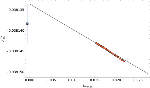
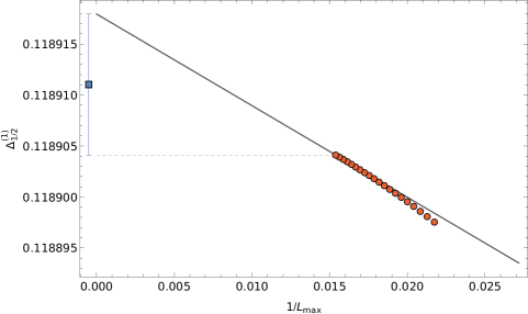
Figure 5: Fitting procedure of anomalous dimensions of the $q=1/2$ monopole $\Delta_{1/2}^{(1)}$ in (a) $\operatorname{QED_{3}}$ ; (b) $\operatorname{QED_{3}-GN}$. The points are obtained with fits $\sum_{i=0}^{k}c_{i;k;L_{\max}}L^{-i}$ with $L\in[L_{\max}-5,L_{\max}]$. The solid line is a linear fit in $1/L_{\max}$ with $L_{\max}\in$[61, 65]. The point with the error bar corresponds to the anomalous dimension computed with Eq.(I.1) and shown in Eq. (I.2)

To further characterize the effect that the size of $L_{\max}$ has on the anomalous dimensions, we also consider the cases $q=1,3/2$ and $q=25/2$ where we used a cutoff $L_{\max}=45+\lfloor q\rceil$. For those charges obtained with a larger cutoff, we can restrain our dataset and obtain the anomalous dimensions with $L_{\max}=35+\lfloor q\rceil$. The results with $L_{\max}=45+\lfloor q\rceil$ are slightly more precise and very similar to those with $L_{\max}=35+\lfloor q\rceil$. As shown in Fig. 6, the drift of the anomalous dimension as $L_{\max}$ is increased is very small relatively to the estimated errors, which indicates the stability of our method.

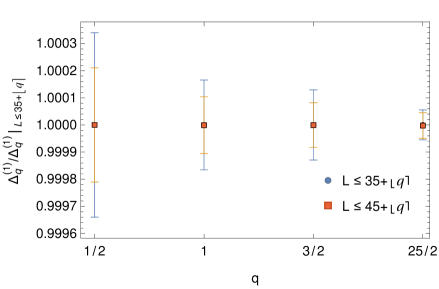
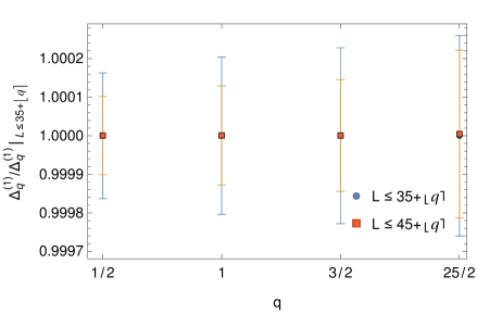
Figure 6: Normalized anomalous dimensions in (a) $\operatorname{QED_{3}}$ ; (b) $\operatorname{QED_{3}-GN}$. There are two sets of scaling dimensions obtained for $L_{\max}\in[31+\lfloor q\rceil,35+\lfloor q\rceil]$ ($L\leq 35+\lfloor q\rceil$) and $L_{\max}\in[41+\lfloor q\rceil,45+\lfloor q\rceil]$ ($L\leq 45+\lfloor q\rceil$). The anomalous dimensions are normalized as $\Delta_{q}^{(1)}/\Delta_{q}^{(1)}|_{L\leq 35+\lfloor q\rceil}$.

The same procedure was also used for different fitting functions $\sum_{i=0}^{k}c_{i;k;L_{\max}}L^{-i}$ with higher polynomial order $k=5,6$, as shown in Fig. 7. We find a similar behaviour and more precise results. However, these fits demand a larger dataset. For larger $q$ (and therefore larger maximal cutoff since the cutoff increases with $\lceil q\rceil$), a similar behaviour remains. However, the size of datasets needs to be increased. This was also observed for $q=1/2$ when comparing relativistic cutoffs $L_{\max}$ of different sizes. It may indicate that errors are overfitted for smaller datasets with higher-order fits, as the effect is less important for $k=4$. We used the quartic fit for all of the anomalous dimensions quoted in this work.

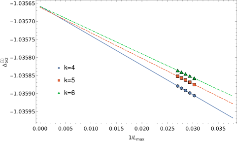
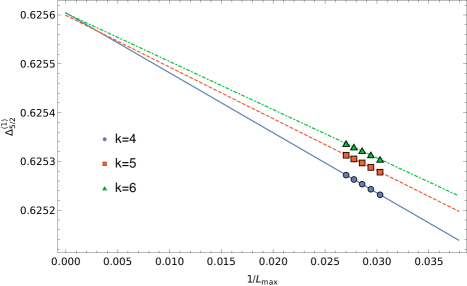
Figure 7: Fitting procedure for anomalous dimensions of the $q=5/2$ monopole $\Delta_{5/2}^{(1)}$ in (a) $\operatorname{QED_{3}}$ ; (b) $\operatorname{QED_{3}-GN}$. The points are obtained with fits $\sum_{i=0}^{k}c_{i;k;L_{\max}}L^{-i}$ with $L\in[L_{\max}-\delta_{k},L_{\max}]$ with $\delta_{k}=\{5,10,14\}$ for $k=\{4,5,6$}. Each set of five points is obtained by varying $L_{\max}\in$[33, 37]. Solid, dashed, and dot-dashed lines are linear fits in $1/L_{\max}$ of the $k=4,5,6$ results.

Appendix J Monopole scaling dimensions for $1/2\leq q\leq 13$

Table 5: Scaling dimension of monopole operators at leading-order and next-to-leading order in $1/N$ in $\operatorname{QED_{3}}$, $\operatorname{QED_{3}-GN}$ and $\operatorname{QED_{3}-Z_{2}GN}$ models. The leading-order result is the same in all models. The scaling dimension is $2N\Delta_{q}^{(0)}+\Delta_{q}^{(1)}$.

$q$	$\Delta_{q}^{(0)}$	$\Delta_{q,\operatorname{QED_{3}}}^{(1)}$	$\Delta_{q,\operatorname{QED_{3}-GN}}^{(1)}$	$\Delta_{q,\operatorname{QED_{3}-Z_{2}GN}}^{(1)}$
$1/2$	$0.26510$	$-0.038138(5)$	$0.118911(7)$	$0.102846(9)$
$1$	$0.67315$	$-0.19340(3)$	$0.23561(4)$	$0.18663(4)$
$3/2$	$1.18643$	$-0.42109(4)$	$0.35808(6)$	$0.26528(7)$
$2$	$1.78690$	$-0.70482(9)$	$0.4879(2)$	$0.3426(2)$
$5/2$	$2.46345$	$-1.0358(2)$	$0.6254(2)$	$0.4202(3)$
$3$	$3.20837$	$-1.4082(2)$	$0.7705(3)$	$0.4989(3)$
$7/2$	$4.01591$	$-1.8181(2)$	$0.9229(3)$	$0.5789(4)$
$4$	$4.88154$	$-2.2623(3)$	$1.0824(4)$	$0.6605(4)$
$9/2$	$5.80161$	$-2.7384(3)$	$1.2488(4)$	$0.7439(5)$
$5$	$6.77309$	$-3.2445(3)$	$1.4218(5)$	$0.8290(6)$
$11/2$	$7.79338$	$-3.7788(4)$	$1.6013(5)$	$0.9160(6)$
$6$	$8.86025$	$-4.3401(4)$	$1.7869(6)$	$1.0048(7)$
$13/2$	$9.97175$	$-4.9269(4)$	$1.9786(7)$	$1.0955(8)$

$q$ $\Delta_{q}^{(0)}$ $\Delta_{q,\operatorname{QED_{3}}}^{(1)}$ $\Delta_{q,\operatorname{QED_{3}-GN}}^{(1)}$ $\Delta_{q,\operatorname{QED_{3}-Z_{2}GN}}^{(1)}$ $7$ $11.12616$ $-5.5384(5)$ $2.1762(7)$ $1.1881(8)$ $15/2$ $12.32195$ $-6.1735(5)$ $2.3794(7)$ $1.2825(9)$ $8$ $13.55772$ $-6.8314(5)$ $2.5882(8)$ $1.3787(9)$ $17/2$ $14.83223$ $-7.5113(6)$ $2.8024(9)$ $1.477(1)$ $9$ $16.14432$ $-8.2125(6)$ $3.0219(9)$ $1.577(2)$ $19/2$ $17.49296$ $-8.9345(6)$ $3.2466(9)$ $1.678(2)$ $10$ $18.87719$ $-9.6766(7)$ $3.476(1)$ $1.781(2)$ $21/2$ $20.29609$ $-10.4383(7)$ $3.711(2)$ $1.886(2)$ $11$ $21.74886$ $-11.2191(7)$ $3.950(2)$ $1.993(2)$ $23/2$ $23.23472$ $-12.0186(7)$ $4.195(2)$ $2.102(2)$ $12$ $24.75294$ $-12.8363(8)$ $4.444(2)$ $2.212(2)$ $25/2$ $26.30286$ $-13.6719(8)$ $4.697(2)$ $2.323(2)$ $13$ $27.88383$ $-14.5249(8)$ $4.955(2)$ $2.437(2)$

References

- Polyakov [1975] A. M. Polyakov, Physics Letters B 59, 82 (1975), ISSN 0370-2693, URL http://www.sciencedirect.com/science/article/pii/0370269375901628.
- Polyakov [1977] A. M. Polyakov, Nuclear Physics B 120, 429 (1977), ISSN 0550-3213, URL http://www.sciencedirect.com/science/article/pii/0550321377900864.
- Hastings [2000] M. B. Hastings, Phys. Rev. B 63, 014413 (2000), URL https://link.aps.org/doi/10.1103/PhysRevB.63.014413.
- Ran et al. [2007] Y. Ran, M. Hermele, P. A. Lee, and X.-G. Wen, Phys. Rev. Lett. 98, 117205 (2007), URL https://link.aps.org/doi/10.1103/PhysRevLett.98.117205.
- Iqbal et al. [2011] Y. Iqbal, F. Becca, and D. Poilblanc, Phys. Rev. B 84, 020407 (2011), URL https://link.aps.org/doi/10.1103/PhysRevB.84.020407.
- Iqbal et al. [2013] Y. Iqbal, F. Becca, S. Sorella, and D. Poilblanc, Phys. Rev. B 87, 060405 (2013), URL https://link.aps.org/doi/10.1103/PhysRevB.87.060405.
- He et al. [2017] Y.-C. He, M. P. Zaletel, M. Oshikawa, and F. Pollmann, Phys. Rev. X 7, 031020 (2017), URL https://link.aps.org/doi/10.1103/PhysRevX.7.031020.
- Liao et al. [2017] H. J. Liao, Z. Y. Xie, J. Chen, Z. Y. Liu, H. D. Xie, R. Z. Huang, B. Normand, and T. Xiang, Phys. Rev. Lett. 118, 137202 (2017), URL https://link.aps.org/doi/10.1103/PhysRevLett.118.137202.
- Kaneko et al. [2014] R. Kaneko, S. Morita, and M. Imada, Journal of the Physical Society of Japan 83, 093707 (2014), eprint https://doi.org/10.7566/JPSJ.83.093707, URL https://doi.org/10.7566/JPSJ.83.093707.
- Iqbal et al. [2016] Y. Iqbal, W.-J. Hu, R. Thomale, D. Poilblanc, and F. Becca, Phys. Rev. B 93, 144411 (2016), URL https://link.aps.org/doi/10.1103/PhysRevB.93.144411.
- Hu et al. [2019] S. Hu, W. Zhu, S. Eggert, and Y.-C. He, Phys. Rev. Lett. 123, 207203 (2019), URL https://link.aps.org/doi/10.1103/PhysRevLett.123.207203.
- Corboz et al. [2012] P. Corboz, M. Lajkó, A. M. Läuchli, K. Penc, and F. Mila, Phys. Rev. X 2, 041013 (2012), URL https://link.aps.org/doi/10.1103/PhysRevX.2.041013.
- Calvera and Wang [2021] V. Calvera and C. Wang, Theory of dirac spin-orbital liquids: monopoles, anomalies, and applications to honeycomb models (2021), eprint 2103.13405.
- Calvera and Wang [2020] V. Calvera and C. Wang, Theory of dirac spin liquids on spin- triangular lattice: possible application to -crooh(d) (2020), eprint 2012.09809.
- Borokhov et al. [2002] V. Borokhov, A. Kapustin, and X. Wu, Journal of High Energy Physics 2002, 049 (2002), URL https://doi.org/10.1088/1126-6708/2002/11/049.
- Pufu [2014] S. S. Pufu, Phys. Rev. D 89, 065016 (2014), URL https://link.aps.org/doi/10.1103/PhysRevD.89.065016.
- Karthik and Narayanan [2019] N. Karthik and R. Narayanan, Phys. Rev. D 100, 054514 (2019), URL https://link.aps.org/doi/10.1103/PhysRevD.100.054514.
- Chester and Pufu [2016] S. M. Chester and S. S. Pufu, Journal of High Energy Physics 2016, 69 (2016), ISSN 1029-8479, URL https://doi.org/10.1007/JHEP08(2016)069.
- Chester et al. [2018] S. M. Chester, L. V. Iliesiu, M. Mezei, and S. S. Pufu, Journal of High Energy Physics 2018 (2018), ISSN 1029-8479, URL http://link.springer.com/10.1007/JHEP05(2018)157.
- Dey [2020] S. Dey, Phys. Rev. B 102, 235165 (2020), URL https://link.aps.org/doi/10.1103/PhysRevB.102.235165.
- Read and Sachdev [1989] N. Read and S. Sachdev, Phys. Rev. Lett. 62, 1694 (1989), URL https://link.aps.org/doi/10.1103/PhysRevLett.62.1694.
- Read and Sachdev [1990] N. Read and S. Sachdev, Phys. Rev. B 42, 4568 (1990), URL https://link.aps.org/doi/10.1103/PhysRevB.42.4568.
- Senthil et al. [2004] T. Senthil, L. Balents, S. Sachdev, A. Vishwanath, and M. P. A. Fisher, Phys. Rev. B 70, 144407 (2004), URL https://link.aps.org/doi/10.1103/PhysRevB.70.144407.
- Senthil et al. [2005] T. Senthil, L. Balents, S. Sachdev, A. Vishwanath, and M. P. A. Fisher, Journal of the Physical Society of Japan 74, 1 (2005), eprint https://doi.org/10.1143/JPSJS.74S.1, URL https://doi.org/10.1143/JPSJS.74S.1.
- Murthy and Sachdev [1990] G. Murthy and S. Sachdev, Nuclear Physics B 344, 557 (1990).
- Atiyah and Singer [1963] M. F. Atiyah and I. M. Singer, Bulletin of the American Mathematical Society 69, 422 (1963), URL https://doi.org/.
- Song et al. [2019] X.-Y. Song, C. Wang, A. Vishwanath, and Y.-C. He, Nature Communications 10, 4254 (2019), ISSN 2041-1723, URL https://doi.org/10.1038/s41467-019-11727-3.
- Ghaemi and Senthil [2006] P. Ghaemi and T. Senthil, Phys. Rev. B 73, 054415 (2006), URL https://link.aps.org/doi/10.1103/PhysRevB.73.054415.
- Hermele et al. [2008] M. Hermele, Y. Ran, P. A. Lee, and X.-G. Wen, Phys. Rev. B 77, 224413 (2008), URL https://link.aps.org/doi/10.1103/PhysRevB.77.224413.
- Lu et al. [2017] Y.-M. Lu, G. Y. Cho, and A. Vishwanath, Phys. Rev. B 96, 205150 (2017), URL https://link.aps.org/doi/10.1103/PhysRevB.96.205150.
- Dupuis et al. [2019] É. Dupuis, M. B. Paranjape, and W. Witczak-Krempa, Phys. Rev. B 100, 094443 (2019), URL https://link.aps.org/doi/10.1103/PhysRevB.100.094443.
- Dupuis et al. [2021] É. Dupuis, M. B. Paranjape, and W. Witczak-Krempa, in Quantum Theory and Symmetries, edited by M. B. Paranjape, R. MacKenzie, Z. Thomova, P. Winternitz, and W. Witczak-Krempa (Springer International Publishing, Cham, 2021), pp. 327–336, ISBN 978-3-030-55777-5.
- Dupuis and Witczak-Krempa [2021] É. Dupuis and W. Witczak-Krempa, Annals of Physics p. 168496 (2021), ISSN 0003-4916, URL https://www.sciencedirect.com/science/article/pii/S0003491621001020.
- Zou et al. [2021] L. Zou, Y.-C. He, and C. Wang, Stiefel liquids: possible non-lagrangian quantum criticality from intertwined orders (2021), eprint 2101.07805.
- He et al. [2015] Y.-C. He, Y. Fuji, and S. Bhattacharjee, Kagome spin liquid: a deconfined critical phase driven by gauge fluctuation (2015), eprint arXiv:1512.05381.
- Janssen and He [2017] L. Janssen and Y.-C. He, Phys. Rev. B 96, 205113 (2017), URL https://link.aps.org/doi/10.1103/PhysRevB.96.205113.
- He et al. [2014] Y.-C. He, D. N. Sheng, and Y. Chen, Phys. Rev. Lett. 112, 137202 (2014), URL https://link.aps.org/doi/10.1103/PhysRevLett.112.137202.
- Gong et al. [2014] S.-S. Gong, W. Zhu, and D. N. Sheng, Scientific Reports 4, 6317 (2014), ISSN 2045-2322, URL https://doi.org/10.1038/srep06317.
- He and Chen [2015] Y.-C. He and Y. Chen, Phys. Rev. Lett. 114, 037201 (2015), URL https://link.aps.org/doi/10.1103/PhysRevLett.114.037201.
- Zhu et al. [2015] W. Zhu, S. S. Gong, and D. N. Sheng, Phys. Rev. B 92, 014424 (2015), URL https://link.aps.org/doi/10.1103/PhysRevB.92.014424.
- Hu et al. [2016] W.-J. Hu, S.-S. Gong, and D. N. Sheng, Phys. Rev. B 94, 075131 (2016), URL https://link.aps.org/doi/10.1103/PhysRevB.94.075131.
- Gong et al. [2017] S.-S. Gong, W. Zhu, J.-X. Zhu, D. N. Sheng, and K. Yang, Phys. Rev. B 96, 075116 (2017), URL https://link.aps.org/doi/10.1103/PhysRevB.96.075116.
- Wietek and Läuchli [2017] A. Wietek and A. M. Läuchli, Phys. Rev. B 95, 035141 (2017), URL https://link.aps.org/doi/10.1103/PhysRevB.95.035141.
- Ihrig et al. [2018] B. Ihrig, L. Janssen, L. N. Mihaila, and M. M. Scherer, Phys. Rev. B 98, 115163 (2018), URL https://link.aps.org/doi/10.1103/PhysRevB.98.115163.
- Gracey [2018] J. A. Gracey, Phys. Rev. D 98, 085012 (2018), URL https://link.aps.org/doi/10.1103/PhysRevD.98.085012.
- Zerf et al. [2018] N. Zerf, P. Marquard, R. Boyack, and J. Maciejko, Phys. Rev. B 98, 165125 (2018), URL https://link.aps.org/doi/10.1103/PhysRevB.98.165125.
- Boyack et al. [2019] R. Boyack, A. Rayyan, and J. Maciejko, Phys. Rev. B 99, 195135 (2019), URL https://link.aps.org/doi/10.1103/PhysRevB.99.195135.
- Benvenuti and Khachatryan [2019a] S. Benvenuti and H. Khachatryan, Journal of High Energy Physics 2019, 214 (2019a), ISSN 1029-8479, URL https://doi.org/10.1007/JHEP05(2019)214.
- Zerf et al. [2016] N. Zerf, C.-H. Lin, and J. Maciejko, Phys. Rev. B 94, 205106 (2016), URL https://link.aps.org/doi/10.1103/PhysRevB.94.205106.
- Boyack et al. [2018] R. Boyack, C.-H. Lin, N. Zerf, A. Rayyan, and J. Maciejko, Phys. Rev. B 98, 035137 (2018), URL https://link.aps.org/doi/10.1103/PhysRevB.98.035137.
- Lu et al. [2011] Y.-M. Lu, Y. Ran, and P. A. Lee, Phys. Rev. B 83, 224413 (2011), URL https://link.aps.org/doi/10.1103/PhysRevB.83.224413.
- Roy et al. [2013] B. Roy, V. Juričić, and I. F. Herbut, Phys. Rev. B 87, 041401 (2013), URL https://link.aps.org/doi/10.1103/PhysRevB.87.041401.
- Wang et al. [2017] C. Wang, A. Nahum, M. A. Metlitski, C. Xu, and T. Senthil, Phys. Rev. X 7, 031051 (2017), URL https://link.aps.org/doi/10.1103/PhysRevX.7.031051.
- Hellerman et al. [2015] S. Hellerman, D. Orlando, S. Reffert, and M. Watanabe, Journal of High Energy Physics 2015, 1 (2015), ISSN 1029-8479, eprint arXiv:1505.01537, URL https://doi.org/10.1007/JHEP12(2015)071.
- Heras [2018] R. Heras, Contemporary Physics 59, 331 (2018), URL https://doi.org/10.1080/00107514.2018.1527974.
- Metlitski et al. [2008] M. A. Metlitski, M. Hermele, T. Senthil, and M. P. A. Fisher, Phys. Rev. B 78, 214418 (2008), URL https://link.aps.org/doi/10.1103/PhysRevB.78.214418.
- Rantner and Wen [2002] W. Rantner and X.-G. Wen, Phys. Rev. B 66, 144501 (2002), URL https://link.aps.org/doi/10.1103/PhysRevB.66.144501.
- Hermele et al. [2005] M. Hermele, T. Senthil, and M. P. A. Fisher, Phys. Rev. B 72, 104404 (2005), URL https://link.aps.org/doi/10.1103/PhysRevB.72.104404.
- Wu and Yang [1976] T. T. Wu and C. N. Yang, Nuclear Physics B 107, 365 (1976), ISSN 0550-3213, URL https://www.sciencedirect.com/science/article/pii/0550321376901437.
- Wu and Yang [1977] T. T. Wu and C. N. Yang, Phys. Rev. D 16, 1018 (1977), URL https://link.aps.org/doi/10.1103/PhysRevD.16.1018.
- Dyer et al. [2013] E. Dyer, M. Mezei, and S. S. Pufu, Monopole taxonomy in three-dimensional conformal field theories (2013), eprint arXiv:1309.1160.
- Pufu and Sachdev [2013] S. S. Pufu and S. Sachdev, Journal of High Energy Physics 2013 (2013), ISSN 1029-8479, URL http://link.springer.com/10.1007/JHEP09(2013)127.
- Dyer et al. [2015] E. Dyer, M. Mezei, S. S. Pufu, and S. Sachdev, Journal of High Energy Physics 2015 (2015), ISSN 1029-8479, URL http://link.springer.com/10.1007/JHEP06(2015)037.
- Dyer et al. [2016] E. Dyer, M. Mezei, S. S. Pufu, and S. Sachdev, Journal of High Energy Physics 2016, 111 (2016), ISSN 1029-8479, URL https://doi.org/10.1007/JHEP03(2016)111.
- Aharony and Palti [2021] O. Aharony and E. Palti, On convexity of charged operators in cfts and the weak gravity conjecture (2021), eprint 2108.04594.
- Cuomo [2021] G. Cuomo, Physics Letters B 812, 136014 (2021), ISSN 0370-2693, URL https://www.sciencedirect.com/science/article/pii/S0370269320308170.
- Monin [2016] A. Monin, Physical Review D 94 (2016), ISSN 2470-0029, URL http://dx.doi.org/10.1103/PhysRevD.94.085013.
- de la Fuente [2018] A. de la Fuente, Journal of High Energy Physics 2018, 41 (2018), ISSN 1029-8479, URL https://doi.org/10.1007/JHEP08(2018)041.
- Benvenuti and Khachatryan [2019b] S. Benvenuti and H. Khachatryan, Qed’s in dimensions: complex fixed points and dualities (2019b), eprint 1812.01544.
- Bartosch [2013] L. Bartosch, Phys. Rev. B 88, 195140 (2013), URL https://link.aps.org/doi/10.1103/PhysRevB.88.195140.
- Sandvik [2007] A. W. Sandvik, Phys. Rev. Lett. 98, 227202 (2007), URL https://link.aps.org/doi/10.1103/PhysRevLett.98.227202.
- Melko and Kaul [2008] R. G. Melko and R. K. Kaul, Phys. Rev. Lett. 100, 017203 (2008), URL https://link.aps.org/doi/10.1103/PhysRevLett.100.017203.
- Kaul and Sandvik [2012] R. K. Kaul and A. W. Sandvik, Phys. Rev. Lett. 108, 137201 (2012), URL https://link.aps.org/doi/10.1103/PhysRevLett.108.137201.
- Pujari et al. [2013] S. Pujari, K. Damle, and F. Alet, Phys. Rev. Lett. 111, 087203 (2013), URL https://link.aps.org/doi/10.1103/PhysRevLett.111.087203.
- Nahum et al. [2015] A. Nahum, J. T. Chalker, P. Serna, M. Ortuño, and A. M. Somoza, Phys. Rev. X 5, 041048 (2015), URL https://link.aps.org/doi/10.1103/PhysRevX.5.041048.
- Halperin et al. [1974] B. I. Halperin, T. C. Lubensky, and S.-k. Ma, Phys. Rev. Lett. 32, 292 (1974), URL https://link.aps.org/doi/10.1103/PhysRevLett.32.292.
- Kaul and Sachdev [2008] R. K. Kaul and S. Sachdev, Phys. Rev. B 77, 155105 (2008), URL https://link.aps.org/doi/10.1103/PhysRevB.77.155105.
- Jiang et al. [2008] F.-J. Jiang, M. Nyfeler, S. Chandrasekharan, and U.-J. Wiese, Journal of Statistical Mechanics: Theory and Experiment 2008, P02009 (2008), URL https://doi.org/10.1088/1742-5468/2008/02/p02009.
- Lou et al. [2009] J. Lou, A. W. Sandvik, and N. Kawashima, Phys. Rev. B 80, 180414 (2009), URL https://link.aps.org/doi/10.1103/PhysRevB.80.180414.
- Sandvik and Zhao [2020] A. W. Sandvik and B. Zhao, Chinese Physics Letters 37, 057502 (2020), URL https://doi.org/10.1088/0256-307x/37/5/057502.
- Ihrig et al. [2019] B. Ihrig, N. Zerf, P. Marquard, I. F. Herbut, and M. M. Scherer, Phys. Rev. B 100, 134507 (2019), URL https://link.aps.org/doi/10.1103/PhysRevB.100.134507.
- Pujari et al. [2015] S. Pujari, F. Alet, and K. Damle, Phys. Rev. B 91, 104411 (2015), URL https://link.aps.org/doi/10.1103/PhysRevB.91.104411.
- Li [2021] Z. Li, On conformality and self-duality of qed3 (2021), eprint 2107.09020.
- Qin et al. [2017] Y. Q. Qin, Y.-Y. He, Y.-Z. You, Z.-Y. Lu, A. Sen, A. W. Sandvik, C. Xu, and Z. Y. Meng, Phys. Rev. X 7, 031052 (2017), URL https://link.aps.org/doi/10.1103/PhysRevX.7.031052.
- Ma and Wang [2020] R. Ma and C. Wang, Phys. Rev. B 102, 020407 (2020), URL https://link.aps.org/doi/10.1103/PhysRevB.102.020407.
- Serna and Nahum [2019] P. Serna and A. Nahum, Phys. Rev. B 99, 195110 (2019), URL https://link.aps.org/doi/10.1103/PhysRevB.99.195110.
- Karch and Tong [2016] A. Karch and D. Tong, Phys. Rev. X 6, 031043 (2016), URL https://link.aps.org/doi/10.1103/PhysRevX.6.031043.
- Fu et al. [2007] L. Fu, C. L. Kane, and E. J. Mele, Physical review letters 98, 106803 (2007).
- Yanagisawa and Hase [2012] T. Yanagisawa and I. Hase, Journal of the Physical Society of Japan 81, SB039 (2012).
- Christos et al. [2020] M. Christos, S. Sachdev, and M. S. Scheurer, Proceedings of the National Academy of Sciences 117, 29543 (2020), eprint https://www.pnas.org/doi/pdf/10.1073/pnas.2014691117, URL https://www.pnas.org/doi/abs/10.1073/pnas.2014691117.
- Bernevig and Hughes [2013] B. Bernevig and T. Hughes, Topological Insulators and Topological Superconductors (Princeton University Press, 2013), ISBN 978-0-691-15175-5.
- Xu et al. [2019] X. Y. Xu, Y. Qi, L. Zhang, F. F. Assaad, C. Xu, and Z. Y. Meng, Phys. Rev. X 9, 021022 (2019), URL https://link.aps.org/doi/10.1103/PhysRevX.9.021022.
- Wang et al. [2019] W. Wang, D.-C. Lu, X. Y. Xu, Y.-Z. You, and Z. Y. Meng, Phys. Rev. B 100, 085123 (2019), URL https://link.aps.org/doi/10.1103/PhysRevB.100.085123.
- Zerf et al. [2019] N. Zerf, R. Boyack, P. Marquard, J. A. Gracey, and J. Maciejko, Phys. Rev. B 100, 235130 (2019), URL https://link.aps.org/doi/10.1103/PhysRevB.100.235130.
- Zerf et al. [2020] N. Zerf, R. Boyack, P. Marquard, J. A. Gracey, and J. Maciejko, Phys. Rev. D 101, 094505 (2020), URL https://link.aps.org/doi/10.1103/PhysRevD.101.094505.
- Janssen et al. [2020] L. Janssen, W. Wang, M. M. Scherer, Z. Y. Meng, and X. Y. Xu, Phys. Rev. B 101, 235118 (2020), URL https://link.aps.org/doi/10.1103/PhysRevB.101.235118.
- Boyack and Maciejko [2021] R. Boyack and J. Maciejko, in Quantum Theory and Symmetries. CRM Series in Mathematical Physics, edited by M. B. Paranjape, R. MacKenzie, Z. Thomova, P. Winternitz, and W. Witczak-Krempa (Springer International Publishing, Cham, 2021), pp. 337–345, ISBN 978-3-030-55777-5.
- Sachdev [2012] S. Sachdev, Phys. Rev. D 86, 126003 (2012), URL https://link.aps.org/doi/10.1103/PhysRevD.86.126003.
- Briggs et al. [2013] A. Briggs, H. E. Camblong, and C. R. Ordóñez, International Journal of Modern Physics A 28, 1350047 (2013), eprint https://doi.org/10.1142/S0217751X13500474, URL https://doi.org/10.1142/S0217751X13500474.