Local tropicalizations of splice type surface singularities
Abstract.
Splice type surface singularities were introduced by Neumann and Wahl as a generalization of the class of Pham-Brieskorn-Hamm complete intersections of dimension two. Their construction depends on a weighted tree called a splice diagram. In this paper, we study these singularities from the tropical viewpoint. We characterize their local tropicalizations as the cones over the appropriately embedded associated splice diagrams. As a corollary, we reprove some of Neumann and Wahl’s earlier results on these singularities by purely tropical methods, and show that splice type surface singularities are Newton non-degenerate complete intersections in the sense of Khovanskii. We also confirm that under suitable coprimality conditions on its weights, the diagram can be uniquely recovered from the local tropicalization.
As a corollary of the Newton non-degeneracy property, we obtain an alternative proof of a recent theorem of de Felipe, González Pérez and Mourtada, stating that embedded resolutions of any plane curve singularity can be achieved by a single toric morphism, after re-embedding the ambient smooth surface germ in a higher-dimensional smooth space. The paper ends with an appendix by Jonathan Wahl, providing a criterion of regularity of a sequence in a ring of convergent power series, given the regularity of an associated sequence of initial forms.
Key words and phrases:
Surface singularities, complete intersection singularities, tropical geometry, Newton non-degeneracy2020 Mathematics Subject Classification:
Primary: 14B05, 14T90, 32S05; Secondary: 14M25, 57M15(Published online in Mathematische Annalen on 19 December 2023. https://doi.org/10.1007/s00208-023-02755-y)
1. Introduction
Splice diagrams are finite trees with half-edges weighted by integers and with nodes (internal vertices) decorated by signs. If the half-edge weights around each node are pairwise coprime, we say that the splice diagram is coprime. This class of weighted trees was first introduced by Siebenmann [52] in 1980 to encode graph manifolds which are integral homology spheres. Coprime splice diagrams with only + node decorations and positive half-edge weights were used by Eisenbud and Neumann in [9] to study special kinds of links in integral homology spheres, in particular those corresponding to curves on normal surface singularities with integral homology sphere links. One of the main theorems of [9] states that such integral homology spheres are described by positively-weighted coprime splice diagrams satisfying the edge determinant condition, namely, that the product of the two weights associated to any fixed internal edge must be greater than the product of the weights of the neighboring half-edges.
Interesting isolated surface singularities arise from splice diagrams. For example, complete intersections of Pham-Brieskorn-Hamm hypersurface singularities are associated to star splice diagrams (i.e., those with a single node). As recognized by Hamm in [19, §5] and [20], in order to determine an isolated singularity in , all maximal minors of the coefficient matrix of each polynomial in the Brieskorn system must be non-zero. In turn, work of Neumann [35] shows that universal abelian covers of quasi-homogeneous complex normal surface singularities with rational homology sphere links are complete intersections of Pham-Brieskorn-Hamm hypersurface singularities.
In 2002, Neumann and Wahl [37] extended this family of complete intersections by defining splice type surface singularities associated to splice diagrams whose weights satisfy a special arithmetic property called the semigroup condition. These singularities are defined by explicit splice type systems of convergent power series near the origin, whose coefficients satisfy generalizations of Hamm’s maximal minors conditions. Splice type surface singularities and the related class of splice quotients (determined by diagrams subject to an additional congruence condition) have been further studied by both authors in [38, 39, 40], and by Lamberson, Némethi, Okuma and Pedersen in [27, 31, 32, 33, 42, 43, 44, 46, 47, 48]. For more details, we refer the reader to the surveys [36, 45, 58, 59].
The present paper uses tropical geometry techniques to study splice type systems with leaves associated to splice diagrams satisfying the edge determinant and semigroup conditions. Our first main result recovers and strengthens a central theorem from [38] (see Theorem 2.16). More precisely:
Theorem 1.1.
Splice type systems are Newton non-degenerate complete intersection systems of equations. The associated splice type singularities are isolated, irreducible and not contained in any coordinate subspace of the corresponding ambient space .
This statement plays a major role in the proof of the Neumann-Wahl Milnor fiber conjecture for splice type singularities with integral homology sphere links [39] obtained by the present authors. For an overview of this proof, we refer the reader to [6]. Motivated by Theorem 1.1, we formulate 7.16.
The notion of Newton non-degeneracy (in the sense of Kouchnirenko [25] and Khovanskii [22]) is clossely related to the notion of the initial form of a series relative to a weight vector, which lies at the core of tropical geometry (see Section 3, in particular 3.1). A regular sequence of convergent power series in defining a germ is a Newton non-degenerate complete intersection system if for each weight vector with positive entries, the associated initial forms determine hypersurfaces of the algebraic torus whose sum is a normal crossings divisor in the neighborhood of their intersection. This condition is automatically satisfied whenever the intersection is empty. Surprisingly, not many examples of Newton non-degenerate complete intersection systems are known in codimension two or higher. Theorem 1.1 contributes a large class of examples of such systems.
Newton non-degeneracy enables the resolution of the germ by a single toric morphism. Indeed, works of Varchenko [57] (for hypersurfaces) and Oka [41, Chapter III, Theorem (3.4)] (for complete intersections) show that such a morphism may be defined by a regular subdivision of the positive orthant refining the dual fan of the Newton polyhedron of each function . Furthermore, the complete dual fan is not needed to achieve a resolution. Indeed, [41, Theorem III.3.4] allows us to restrict to the subfan corresponding to the orbits intersecting the strict transform of the given germ.
The support of this subfan depends only on the ideal defining the germ but not on the particular generators . It is the finite part of the so-called local tropicalization of the embedding . This local version of the standard notion of tropicalization of a subvariety of an algebraic torus was first introduced by the last two authors in [49] as a tool to study arbitrary subgerms of or, more generally, arbitrary morphisms from analytic or formal germs to germs of toric varieties.
As was mentioned earlier, splice diagrams record topological information about the link of splice type singularities. Indeed, starting from a normal surface singularity with a rational homology sphere link, Neumann and Wahl [37] build a splice diagram which determines the dual tree of the minimal normal crossings resolution (up to a finite ambiguity) whenever this graph is not a star tree. This diagram is homeomorphic to the dual tree: it is obtained by disregarding all bivalent vertices of the dual tree. It satisfies the edge determinant condition, but not necessarily the semigroup or the congruence conditions. When has an integral homology sphere link, the ambiguity disappears and the dual tree is completely determined by the splice diagram.
Given a splice diagram with leaves, the construction of Neumann and Wahl associates a weight vector to each vertex of . These vectors induce a piecewise linear embedding of into the standard simplex in after appropriate normalization. Our second main result shows the close connection between , the local tropicalization of the associated splice type system in and its resolution diagrams:
Theorem 1.2.
Let be a splice diagram satisfying the semigroup condition and let be the germ defined by an associated splice type system. Then, the finite local tropicalization of is the cone over an embedding of in . Furthermore, in the coprime case, can be uniquely recovered from this fan.
Theorem 1.2 shows that the link at the origin of the local tropicalization of (obtained by intersecting the fan with the -dimensional sphere) is homeomorphic to the splice diagram . To the best of our knowledge, this is the first tropical interpretation of Siebenmann’s splice diagrams. In this spirit, we view Siebenmann’s paper [52] as a precursor to tropical geometry (for others, see [28, Chapter 1]).
Our method to characterize the local tropicalization is different from the general one discussed in Oka’s book [41] and described briefly above. Namely, we do not use the Newton polyhedra of the collection of series defining the germ. Instead, we use a “mine-sweeping” approach, using successive stellar subdivisions of the standard simplex in dictated by the splice diagram, in order to remove relatively open cones in the positive orthant avoiding the local tropicalization.
Once the local tropicalization is determined (via Theorem 1.2), a simple computation confirms the Newton non-degeneracy of the system. In turn, by analyzing the local tropicalizations of the intersections of the germ with the coordinate subspaces of , we conclude that is an isolated complete intersection surface singularity, thus completing the proof of Theorem 1.1.
As a consequence of Theorem 1.1, we provide an alternative proof of the main theorem of de Felipe, González Pérez and Mourtada [11], stating that any germ of a reduced plane curve may be resolved by one toric modification after re-embedding its ambient smooth germ of surface into a higher-dimensional germ (see 7.14). The first theorem of this kind was proved by Goldin and Teissier [17] for irreducible germs of plane curves.
Our paper is organized as follows. In Section 2, we review the definitions and main properties of splice diagrams, splice type systems and end-curves associated to rooted splice diagrams, following [38, 39]. Sections 3 and 4 include background material about local tropicalizations and Newton non-degeneracy. In Section 5 we show how to embed a given splice diagram with leaves into the standard -simplex in , and we highlight various convexity properties of this embedding. The proof of the first part of Theorem 1.2 is discussed in Section 6, while Theorem 1.1 is proven in Section 7. Section 8 characterizes local tropicalizations of splice type systems defined by a coprime splice diagram and shows how to recover the diagram from the tropical fan, thus yielding the second part of Theorem 1.2. Finally, Section 9 discusses the dependency of the construction of splice type systems on the choice of admissible monomials for arbitrary splice diagrams, in the spirit of [38, Section 10].
Appendix A, written by Jonathan Wahl, includes a proof of [38, Lemma 3.3] that was absent from the literature. This result confirms that given a finite sequence in and a fixed positive integer vector , the regularity of the sequence of initial forms ensures that the original sequence is regular, and furthermore, that the -initial ideal must be generated by the sequence of initial forms. This statement can be used to determine if a given lies in the local tropicalization of the germ defined by the vanishing of the input sequence (see 7.7), providing an alternative proof to part of Theorem 1.2.
2. Splice diagrams, splice type systems and end-curves from rooted splice diagrams
In this section, we recall the notions of splice diagram and splice type systems associated to them. The definitions follow closely the work of Neumann and Wahl [38, 39].
We start with some basic terminology and notations about trees:
Definition 2.1.
A tree is a finite connected graph with no cycles and at least one vertex. The star of a vertex of the tree is the set of edges adjacent to . The valency of is the cardinality of , which we denote by . A node of a tree is a vertex whose valency is greater than one, whereas a leaf is a one-valent vertex. We denote the set of nodes of by and its set of leaves by .
When the ambient tree is understood from context, we remove it from the notation and simply write .
Remark 2.2.
Endowing a tree with a metric allows us to consider geodesics on it and distances between vertices. Whenever these notions are invoked, it is understood that each edge of the tree has length one.
Definition 2.3.
Given a subset of vertices of the tree , we denote by or the subtree of spanned by these points. We call it the convex hull of the set inside . For example, .
Splice diagrams are special kinds of trees enriched with weights around all nodes, as we now describe:
Definition 2.4.
A splice diagram is a pair , where is a tree without valency-two vertices, with at least one node, and decorated with a weight function on the star of each node of , denoted by
We call the weight of at . If is any other vertex of such that lies in the unique geodesic of joining and , we write . We view this as the weight in the neighborhood of pointing towards . The total weight of a node of is the product .
Remark 2.5.
Let be a splice diagram. For simplicity, we remove the collection of weights from the notation and simply use to refer to the splice diagram. By a similar abuse of notation, we may view also as a splice diagram, whose weights around its unique node are inherited from . Splice diagrams with one node will be referred to as star splice diagrams, and the underlying graphs as star trees.
Definition 2.6.
Let and be two distinct vertices of the splice diagram . The linking number between and is the product of all the weights adjacent to, but not on, the geodesic joining and . Thus, . We set for each node of . The reduced linking number is defined via a similar product where we exclude the weights around and . In particular, for each node of .
Remark 2.7.
Given a node and a leaf of , it is immediate to check that .
Linking numbers satisfy the following useful identity, whose proof is immediate from 2.6 (see [13, Proposition 69]):
Lemma 2.8.
If are vertices of with , then .
In [34, Theorem 1], Neumann gave explicit descriptions of integral homology spheres associated to star splice diagrams as links of Pham-Brieskorn-Hamm surface singularities. The following definition was introduced by Neumann and Wahl in [39, Section 1] to characterize which integral homology spheres may be realized as links of normal surface singularities. Its origins can be traced back to [9, page 82].
Definition 2.9.
Let be a splice diagram. Given two adjacent nodes and of , the determinant of the edge is the difference between the product of the two decorations on and the product of the remaining decorations in the neighborhoods of and , that is,
| (2.1) |
The splice diagram satisfies the edge determinant condition if all edges have positive determinants.
The next result on integral homology sphere links is due to Eisenbud and Neumann (see [9, Theorem 9.4] for details and 8.1 for the meaning of the coprimality condition). It was strengthened by Pedersen in [47, Theorem 1] to address the case of rational homology sphere links:
Theorem 2.10.
The integral homology sphere links of normal surface singularities are precisely the oriented -manifolds associated to coprime splice diagrams which satisfy the edge determinant condition.
The construction of oriented -manifolds from splice diagrams is due to Siebenmann [52]. They are obtained from splicing Seifert-fibered oriented -manifolds associated to each node of along special fibers of their respective Seifert fibration corresponding to the edges of . For each , these special fibers are in bijection with the -many edges adjacent to . Each edge induces a splicing of both and along the oriented fibers corresponding to the edge. These fibers are knots in both Seifert-fibered manifolds and their linking number is precisely (see [9, Thm. 10.1]).
The following result shows that the edge determinant condition yields Cauchy-Schwarz’ type inequalities:
Lemma 2.11.
Assume that the splice diagram satisfies the edge determinant condition. Then,
| (2.2) |
Furthermore, equality holds if and only if .
Proof.
If satisfies the edge determinant condition, then the linking numbers verify the following inequality, which generalizes 2.8. This inequality is reminiscent of the ultrametric condition for dual graphs of arborescent singularities (see [16, Proposition 1.18]):
Proposition 2.12.
Assume that the splice diagram satisfies the edge determinant condition. Then, for all nodes and of , we have . Furthermore, equality holds if and only if .
Proof.
Consider the tree spanned by and and let be the unique node in the intersections of the three geodesics , and . We prove the inequality by a direct calculation. By 2.8 applied to the triples , and , we have:
These expressions combined with the inequality (2.2) applied to the pair yield:
Furthermore, 2.11 confirms that equality is attained if and only if , that is, if and only if lies in the geodesic . This concludes our proof. ∎
Before introducing splice type systems as defined by Neumann and Wahl in [38, 39], we set up notation arising from toric geometry. We write for the number of leaves of the splice diagram (where denotes the cardinality of a finite set) and let be the free abelian group generated by all leaves of . We denote by its dual lattice and write the associated pairing using dot product notation, i.e. whenever and . Fixing a basis for and its dual basis for identifies both lattices with . To each , we associated a variable . We view as the lattice of exponents of monomials in those variables and as the associated lattice of weight vectors.
In addition to defining weights for all leaves of , each node in has an associated weight vector:
| (2.3) |
As was mentioned in Section 1, star splice diagrams with a unique node produce Pham-Brieskorn-Hamm singularities using the monomials . Neumann and Wahl’s splice type systems [38, 39] generalize this construct to diagrams with more than one node. In addition to satisfying the edge determinant condition, must have an extra arithmetic property that allows to replace each monomial by a suitable monomial associated to the pair where is any node and is an edge adjacent to it (see (2.7)). This property, which ensures that all monomials associated to a vertex have the same -degree, will automatically hold for star splice diagrams.
Definition 2.13.
A splice diagram satisfies the semigroup condition if for each node and each edge , the total weight of belongs to the subsemigroup of generated by the set of linking numbers between and the leaves seen from in the direction of , that is, such that . Therefore, we may write:
| (2.4) |
where for all and is the set of leaves of with .
Assume that satisfies the semigroup condition and pick coefficients satisfying (2.4). Using these integers we define an exponent vector (i.e., an element of ) for each pair as above:
| (2.5) |
Following [39], we refer to it as an admissible exponent for . Note that the relation (2.4) is equivalent to:
| (2.6) |
Each admissible exponent defines an admissible monomial, which was denoted by in [39]:
| (2.7) |
Definition 2.14.
Let be a splice diagram which satisfies both the edge determinant and the semigroup conditions of Definitions 2.9 and 2.13. We fix an order for its set of leaves.
-
•
A strict splice type system associated to is a finite family of polynomials of the form:
(2.8) where are the admissible exponent vectors defined by (2.5) for each node and each edge . We also require the coefficients to satisfy the Hamm determinant conditions. Namely, for any node , if we fix an ordering of the edges in , then all the maximal minors of the matrix of coefficients must be non-zero.
-
•
A splice type system associated to is a finite family of power series of the form
(2.9) where the collection is a strict splice type system associated to and each is a convergent power series satisfying the following condition for each exponent in the support of :
(2.10) -
•
A splice type singularity associated to is the subgerm of defined by .
Remark 2.15.
The inequalities in (2.10) should be compared with the equality imposed in (2.6). As was shown by Neumann and Wahl in [38, Lemma 3.2], the right-most inequality in (2.10) follows from the left-most one and the edge determinant condition. We choose to include both inequalities in (2.10) for mere convenience since we will need both of them for several arguments in Section 6.
The issue of dependency of the set of germs defined by splice type systems on the choice of admissible monomials is a subtle one. We postpone this discussion to Section 9.
As was mentioned in Section 1, splice type singularities satisfy the following crucial property, proved by Neumann and Wahl in [38, Thm. 2.6]. An alternative proof of this statement, using local tropicalization, will be provided at the end of Section 7.
Theorem 2.16.
Splice type singularities are isolated complete intersection surface singularities.

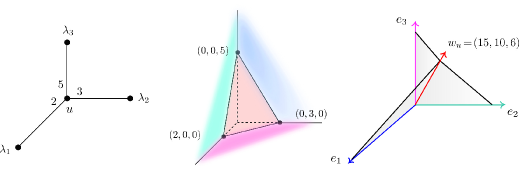
Example 2.16.
We let be the splice diagram to the left of Figure 1. Then, , and and so the edge determinant condition holds for .
The semigroup condition is also satisfied, since
Thus, we may take as exponents and or in . A possible strict splice type system for is:
| (2.11) |
An alternative system is obtained by replacing the admissible monomial with . The coefficients of the system were chosen to simplify the parameterization of the end-curve of the corresponding splice type surface singularity associated to the leaf (see Section 2 for details).
A central role in this paper will be played by tropicalizations and weighted initial forms of series and ideals of , which we discuss in Section 3. In 7.1, we determine the initial forms of the series of a splice type system with respect to each weight vector from (2.3). Its proof is a consequence of the next two lemmas:
Lemma 2.17.
Assume that is a splice diagram satisfying the edge determinant condition. Then, for any pair of adjacent nodes of we have:
Proof.
We write . The definition of linking numbers gives the following expressions for each :
The statement follows by substituting these expressions in the definition of from (2.3) and by using the edge determinant condition, i.e.,
| (2.12) |
Lemma 2.18.
Assume that satisfies the edge determinant and semigroup conditions. Then, the exponent vector from (2.5) satisfies for all nodes of and each edge . Furthermore, equality holds if and only if .
Proof.
If , then . If , we argue by induction on the distance between and in the tree . If , we let . Expression (2.12) yields
The second summand is always non-negative and it equals zero if and only if .
In Section 7, we will be interested in curves obtained from a given splice type system when we choose a leaf of the corresponding splice diagram to be its root. We orient the resulting rooted tree towards the root and remove one weight in the neighborhood of each node, namely the one pointing towards the root, as seen on the right of Figure 1. We write for the set of non-root leaves of and assume it is ordered. The following definition was introduced in [38, Section 3] by the name of splice diagram curves.
Definition 2.19.
Assume that the rooted splice diagram satisfies the semigroup condition and consider a fixed strict splice type system associated to the (unrooted) splice diagram . For each node of and each index , we let be the polynomial obtained from by removing the term corresponding to the unique edge adjacent to pointing towards . The subvariety of defined by the vanishing of is called the end-curve of relative to . We denote it by .
A planar embedding of determines an ordering of the edges adjacent to a fixed node that point away from (for example, by reading them from left to right). Once this order is fixed, by the Hamm determinant conditions, each group of equations becomes equivalent to a collection of -homogeneous binomial equations of the form
with all . The next statement summarizes the main properties of discussed in [38, Theorem 3.1]:
Theorem 2.20.
The subvariety is a reduced complete intersection curve, smooth away from the origin, and meets any coordinate subspace of only at the origin. It has many components, where . All of them are isomorphic to torus-translates of the monomial curve in with parameterization .
Example 2.20.
We fix the splice diagram from Section 2 and consider its rooted analog obtained by setting the first leaf as its root , as seen in the right of Figure 1. By construction, , , , , , , and . The equations defining this end-curve are obtained by removing the monomial indexed by the edge pointing towards in each equation from (2.11). Since , the curve is reduced and irreducible. It is defined as the solution set to
Linear combinations of the last two expressions yield the equivalent binomial system:
An explicit parameterization is given by .
The collection of polynomials defining the end-curve determines a map . Our next result, which we state for comparison’s sake with 7.12, discusses the restriction of this map to each coordinate hyperplane of :
Corollary 2.21.
For every , the restriction of to the hyperplane of defined by the equation is dominant.
Proof.
By Theorem 2.20, the fiber over the origin of the restricted map is finite. Upper semicontinuity of fiber dimensions implies that the generic fiber is also -dimensional. Since , the map must be dominant. ∎
3. Local tropicalization
In [49], the last two authors developed a theory of local tropicalizations of algebraic, analytic or formal germs endowed with maps to (not necessarily normal) toric varieties, adapting the original formulation of global tropicalization (see, e.g. [28]) to the local setting. In this section, we recall the basics on local tropicalizations that will be needed in Section 6. We focus our attention on germs defined by ideals of the ring of convergent power series near the origin, rather than of its completion . As 3.4 confirms, both local tropicalizations yield the same set.
The notion of local tropicalization of an embedded germ is rooted on the construction of initial ideals associated to non-negative weight vectors, which we now describe. Any weight vector induces a real-valued valuation on , known as the -weight, as follows. Given a monomial , we set . In turn, for each with we set
| (3.1) |
We define . The set is called the support of , and it is the basis of the construction of the Newton polyhedron and the Newton fan of (see 3.2).
Definition 3.1.
Given and , the -initial form is the sum of the terms in the series with minimal -weight . In turn, given an ideal of , the -initial ideal of in is generated by the -initial forms of all elements of . If , the -initial ideal of is the ideal of generated by the -initial forms of all elements of .
Example 3.1.
The initial forms of a series determine its Newton fan as follows:
Definition 3.2.
The Newton polyhedron of a non-zero element is the convex hull of the Minkowski sum of and the support of . Given a face of , we let be the closure of the set of weight vectors in supporting (that is, such that the convex hull of the support of is ). The set is the Newton fan of .
The map yields an inclusion-reversing bijection between the set of faces of and the Newton fan . Furthermore, every face of satisfies
| (3.2) |
Definition 3.3.
Let be a germ defined by an ideal of . The local tropicalization of or of the germ , is the set of all vectors such that the -initial ideal of is monomial-free. We denote it by or . In turn, the positive local tropicalization of or of the germ , is the intersection of the local tropicalization with the positive orthant . We denote it by or .
Even though 3.3 depends heavily on the fixed embedding , we omit it from the notation for the sake of simplicity. The next remarks clarify some differences between the present approach and that of [49], which defines local tropicalizations using local valuation spaces (see [49, Definitions 5.13 and 6.7]). A recent extension of this construction to toric prevarieties by means of Berkovich analytification can be found in [26].
Remark 3.4.
As shown in [49, Theorem 11.2] and [54, Corollary 4.3], local tropicalizations of ideals in either or admit several equivalent characterizations analogous to the Fundamental Theorem of Tropical Algebraic Geometry [28, Theorem 3.2.3]. One of them is as Euclidean closures in of images of local valuation spaces. By [49, Corollary 5.17], the canonical inclusion induces an isomorphism of local valuation spaces. This implies that extending an ideal in to the complete ring will yield the same local tropicalization. Therefore, we can define local tropicalizations for ideals of rather than of , in agreement with the setting of splice type systems.
As in the global case, local tropicalizations of hypersurface germs can be obtained from the corresponding Newton fans. Indeed, if the ideal is principal, generated by , and , then each initial ideal is also principal, with generator . Equality (3.2) then yields the following statement (see [49, Proposition 11.8]):
Proposition 3.5.
The set is the union of all cones of the Newton fan of dual to bounded edges of the Newton polyhedron of .
Example 3.5.
The surface singularity is the splice type surface singularity defined by the polynomial . Its associated splice diagram, Newton polyhedron and local tropicalization are depicted in Figure 2. Its local tropicalization is a 2-dimensional fan with four rays spanned by , , , and . Its three maximal cones are spanned by the pairs for . These three cones are dual to the three bounded edges of the Newton polyhedron.
By contrast, if has two or more generators, their -initial forms need not generate . However, for the purpose of characterizing , it is enough to have a tropical basis for in the sense of [49, Definition 10.1], i.e., a finite set of generators of which is a universal standard basis of in the sense of [49, Definition 9.8] and such that for any , the -initial ideal contains a monomial if and only if one of the initial forms is a scalar multiple of a monomial.
Remark 3.6.
Such tropical bases exist by [49, Theorem 10.3] and can be used to determine by intersecting the local tropicalizations of the corresponding hypersurface germs. Furthermore, their existence ensures that local tropicalizations are supports of rational fans in . Indeed, the corresponding fan is obtained by considering the common refinement of the intersection of the local tropicalization of each member of a tropical basis for combined with 3.5. Furthermore, under the hypothesis that no irreducible component of is included in a coordinate subspace of , such fans and their refinements are standard tropicalizing fans of in the sense of 3.14 below.
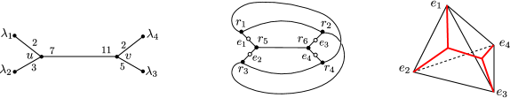
Example 3.6.
We consider the germ of splice type surface singularity from [39, Example 2], given by
| (3.3) |
associated to the splice diagram on the left of Figure 3. A computation with the package Tropical.m2 [1], available in Macaulay2 [18], determines the global tropicalization of the system (see [28, Definition 3.2.1]). It is a 2-dimensional fan in with -vector . Its six rays are generated by the primitive vectors
Notice that and . Its nine top-dimensional cones are encoded by the graph depicted at the center of the figure.
The local tropicalization of the germ defined by (3.3) is obtained by intersecting the global tropicalization with the positive orthant [49, Theorem 12.10]. We indicate the positions of the four canonical basis elements of with unfilled dots inside the edges of the central graph of Figure 3. As we will see in Theorem 6.2, the local tropicalization of this germ can be obtained as the cone over the red graph depicted in the standard tetrahedron seen in the right of the figure. Note that this graph is homeomorphic to the splice diagram. This fact is general, as confirmed by Theorem 5.11.
Remark 3.7.
Our choice of terminology for local tropicalizations differs slightly from [49], as we now explain. As was shown in [49, Section 6], the local tropicalizations of the intersection of a germ with each coordinate subspace of can be glued together to form an extended fan in called the local nonnegative tropicalization of in [49]. In the present paper, we refer to this structure as an extended tropicalization of the germ , in agreement with Kashiwara and Payne’s constructions for global tropicalizations (see [28, §6.2]). The finite part of this extended tropicalization (i.e., its intersection with ) is the local tropicalization from 3.3. A precise description of the boundary strata of the extended local tropicalization of splice type singularities is given in Subsection 6.2.
Remark 3.8.
The local tropicalization of a germ coincides with the local tropicalization of the associated reduced germ since the defining ideal of is the radical and -initial forms respect products. As a consequence, is monomial-free if and only if the same is true for . Alternatively, the same statement can be obtained from the definition of local tropicalization as the image of the local valuation space of and the fact that the embedding induces a homeomorphism of local valuation spaces (see [49, Lemma 5.18]).
Remark 3.9.
The local tropicalization of a reduced germ is equal to the union of the local tropicalizations of its irreducible components, and the same is true for their local positive tropicalizations. This is a direct consequence of the fact that the local valuation space of is the union of the local valuation spaces of its irreducible components (see [49, Lemma 5.18]).
The next result determines the local tropicalization of a germ from the positive one:
Proposition 3.10.
The local tropicalization is the closure of the positive local tropicalization inside the cone .
Proof.
By Remarks 3.8 and 3.9, it suffices to consider the case where is irreducible. In this situation, [49, Theorem 11.9] shows that the extended local tropicalization of is the closure of the extended positive local tropicalization in the extended non-negative orthant . Applying 3.11 below to the case when is the extended local tropicalization of , and is the extended local tropicalization of confirms the claim about the closure of in . ∎
The following lemma is a standard statement in general set topology, which may for instance be obtained as an immediate consequence of [30, Theorem 17.4]:
Lemma 3.11.
Let be a topological space and be an open subset. Then, for any subset of we have:
where is the closure of in and denotes the closure of in .
In what follows, we restrict our attention to subgerms of with no components included in coordinate subspaces. Their local tropicalizations verify the following key property (see [49, Proposition 9.21, Theorems 10.3 and 11.9]):
Proposition 3.12.
Let be a subgerm of with no irreducible components contained in coordinate subspaces of , and let be its defining ideal. Then, is the support of a rational polyhedral fan which satisfies the following conditions:
-
(1)
the dimension of all the maximal cones of agrees with the complex dimension of ;
-
(2)
the maximal cones of have non-empty intersections with ;
-
(3)
given any cone of , the -initial ideal of is independent of the choice of .
Proof.
By Remarks 3.8 and 3.9, we may restrict to the case when is reduced and irreducible. The existence of satisfying the first two conditions is a direct consequence of [49, Theorem 11.9], which ensures the analogous properties hold for the extended local tropicalization of . Note that is non-empty, since meets the dense torus of (see [49, Lemma 7.4]). Furthermore, the fan structure on induced from a tropical basis for discussed in 3.6 satisfies condition (3). In turn, any refinement will satisfy conditions (1) and (2) as well. ∎
Remark 3.13.
3.12 allows us to recover the complex dimension of an irreducible germ meeting the dense torus from its positive tropicalization (see, for instance, the proofs of Corollaries 6.20 and 6.21). Indeed, its dimension agrees with the dimension of any of the top-dimensional cones in any fixed fan satisfying conditions (1)–(3) in 3.12. If is not irreducible, a similar procedure determines the maximal dimension of a component of the germ meeting the dense torus.
Definition 3.14.
Let be a subgerm of with no irreducible component contained in a coordinate subspace of . Let be the ideal of defining . Any fan satisfying all three conditions in 3.12 is called a standard tropicalizing fan for or for . For every cone of meeting and any , we write for the associated initial ideal in the polynomial ring and for the associated subscheme of (see 3.1).
Remark 3.15.
When is a hypersurface germ defined by a series , the set of cones of codimension one of the Newton fan of dual to bounded edges of the Newton polyhedron of satisfies all three conditions listed in 3.12. Furthermore, it is the coarsest fan with these properties. However, for germs of higher codimension such canonical choice need not always exist. For an example in the global (i.e., polynomial) setting, we refer the reader to [28, Example 3.5.4].
The next proposition emphasizes the relevance of tropicalizing fans for producing birational models of irreducible germs with desirable geometric properties, in the spirit of Tevelev’s construction of tropical compactifications of subvarieties of tori [56].
Proposition 3.16.
Fix a rational polyhedral fan contained in and let be the associated toric morphism. Given an irreducible germ meeting the dense torus, let be the strict transform of under and write for the restriction of the map to . Then, the following properties hold:
-
(1)
The restriction is proper if and only if the support contains the local tropicalization .
-
(2)
Assume that is proper. Then, the strict transform intersects every orbit of along a non-empty pure-dimensional subvariety with if and only if .
Proof.
In what follows, we use standard terminology and notation from toric geometry, which can be found in Fulton’s book [12]. The proof of (2) is similar to the global analog [28, Proposition 6.4.7 (2)], so we leave it to the reader.
It remains to prove assertion (1). To this end, we consider a fan subdividing the non-negative cone and containing as a subfan. Such a fan exists by [10, Theorem 2.8 (III.2)].
We consider the toric varieties and associated to the fans and and the natural toric morphisms and . We let and be the strict transforms of under these two maps. The aforementioned varieties and maps fit naturally into the commutative diagram
where the central triangle involves toric morphisms and the horizontal arrows are embeddings. The vertical map on the right is the restriction of to . In what follows we view as an open subvariety of . Note that the toric birational morphism is proper by [12, Section 2.4], as the defining fans of its source and target have the same support, namely .
By construction, is proper if and only if is contained in . Thus, claim (1) will follow if we show that for every cone of we have the following equivalence:
| (3.4) |
where is the corresponding toric orbit.
It remains to prove (3.4). We start with the forward implication and fix . Then, there exists a holomorphic arc in parameterized as such that the limit as of its strict transform in equals , i.e.,
Such an arc can be built by choosing an irreducible subgerm of a curve of the germ , not contained in the toric boundary, then by projecting it to a subgerm of via and, finally, by choosing a normalization of , which we identify with .
We consider the weight vector in the dual lattice recording the orders of vanishing of the components of . We claim that belongs to , so , as desired. To prove this claim, notice that the arc of obtained by keeping the -initial terms of the components of has the same limit when as does. This fact can be checked by working in the affine toric variety associated to the cone . Properties of limits in toric varieties from [12, Section 2.3] ensure that is equivalent to the fact that the weight vector lies in . Therefore, we conclude that .
It remains to verify that . To do so, it suffices to notice that (since ) and that . The latter is a direct consequence of [54, Corollary 4.3 3’)] (see also Maurer’s paper [29] which includes a precursor of local tropicalization for germs of space curves).
Finally, to prove the reverse implication of (3.4), we assume that and let be a primitive lattice vector in . We consider a refinement of such that the ray . By construction, the orbit is mapped via the toric morphism to the orbit .
The intersection of with the orbit is determined by the -initial ideal of the ideal defining , viewed in the Laurent polynomial ring. Since this initial ideal is monomial free because , this intersection is non-empty. Since , the map ensures that as well. This concludes our proof. ∎
One well-known feature of global tropicalizations of equidimensional subvarieties of toric varieties is the so-called balancing condition [28, Section 3.3]. To this end, tropical varieties must be endowed with positive integer weights (called tropical multiplicities) along their top-dimensional cones. Such multiplicities may be also defined in the local situation. We restrict the exposition to equidimensional germs, since this is sufficient for the purposes of this paper.
Definition 3.17.
Let be an equidimensional germ meeting , defined by an ideal of and let be a standard tropicalizing fan for it. Given a top-dimensional cone of , we define the tropical multiplicity of at to be the number of irreducible components of , counted with multiplicity.
In order to state the balancing condition for local tropicalization, we first define the notion of a pure rational weighted balanced fan. Recall that a fan is pure if all its top-dimensional cells have the same dimension.
Definition 3.18.
Consider a pure rational polyhedral fan in relative to the lattice , with positive integer weights on its maximal cones. Fix a cone of of codimension one in , and let be the maximal cones of containing as a face. Denote by the corresponding weights. For each consider a vector generating the lattice
| (3.5) |
We say that is balanced at if . The fan is balanced if it is balanced at each of its codimension one cones.
Remark 3.19.
By construction, the lattice in (3.5) is free of rank one. It has one generator, up to sign. Even though there are many choices for , their projections onto give the same generator of the lattice.
Our last statement in this section confirms that the balancing condition holds for local tropicalizations of equidimensional germs in meeting the dense torus . Its validity follows from [49, Remark 11.3, Theorem 12.10]:
Theorem 3.20.
Let be an equidimensional germ meeting and let be any refinement of a standard tropicalizing fan for . Then, is a balanced fan when endowed with tropical multiplicities as in 3.17.
Remark 3.21.
Balancing for local tropicalizations of equidimensional germs of surfaces features in the proof of 6.26. This property will help us prove that the embedded splice diagrams in are included in the local tropicalizations of the corresponding splice type systems (see Subsection 6.3). Tropical multiplicities will be also used in Section 8 to recover the edge weights on any coprime splice diagram from the local tropicalization of any splice type surface singularity associated to it.
4. Newton non-degeneracy
In this section we discuss the notion of Newton non-degenerate complete intersection in the sense of Khovanskii [22], starting with the case of formal power series in , as introduced by Kouchnirenko in [24, Sect. 8] and [25, Def. 1.19]. Kouchnirenko’s definition was later extended by Steenbrink [53, Def. 5] to -algebras of formal power series with exponents on an arbitrary saturated sharp toric monoid . For precursors to this notion we refer the reader to Teissier’s work [55, Section 5].
Definition 4.1.
Given a series , we say that is Newton non-degenerate if for any positive weight vector , the subvariety of the dense torus defined by is smooth.
Example 4.1.
We consider the singularity from Section 3, defined by . Its local tropicalization is depicted in Figure 2. Since is a monomial whenever , the Newton non-degeneracy condition only needs to be checked for .
The calculations are simplified since is a subfan of the normal fan to the Newton polyhedron of . If , we have . In turn, weight vectors in the relative interiors of maximal cones of satisfy
All four initial forms describe surfaces that are smooth when restricted to the torus . Thus, is Newton non-degenerate.
The notion of Newton non-degeneracy extends naturally to finite sequences of functions. For our purposes, it suffices to restrict ourselves to regular sequences, i.e., collections in where
-
(1)
is not a zero divisor of , and
-
(2)
for each , the element is not a zero divisor in the quotient ring .
As is a regular local ring, the germs defined by regular sequences in are exactly formal complete intersections at the origin of .
Definition 4.2.
Fix a positive integer and a regular sequence in . Consider the germ defined by the ideal . The sequence is a Newton non-degenerate complete intersection system for if for any positive weight vector , the hypersurfaces of defined by each form a normal crossings divisor in a neighborhood of their intersection. Equivalently, the differentials of the initial forms must be linearly independent at each point of this intersection.
Remark 4.3.
Notice that 4.2 allows for the initial forms to be monomials. This would determine an empty intersection with the dense torus .
Our main result in this section is a useful tool for proving that a regular sequence in defines a Newton non-degenerate system. We make use of this statement in Theorem 7.3:
Proposition 4.4.
Let be a positive integer, be a sequence in and be a weight vector in . Assume that is a regular sequence in defining a subscheme of . If is a smooth point of , then the differentials at of the initial forms are linearly independent.
Proof.
Fix any point . Our regularity hypothesis implies that . Since is a smooth point of , by [7, Lemma 4.3.5] we know that is a regular local ring of dimension . Furthermore, this quantity equals the embedding dimension of the local ring .
In turn, the Jacobian criterion for smoothness (see, e.g., [7, Theorem 4.3.6]) enables us to compute the rank of the Jacobian matrix of the initial forms evaluated at , in terms of and this embedding dimension. More precisely, we have
This implies that the differentials of the initial forms are linearly independent at . ∎
Example 4.4.
We consider the splice type system from Section 3. As claimed by Theorem 1.1, the germ defined by it is Newton non-degenerate. By 4.3 we need only focus on weights . A direct computation using 2.18 shows that the initial forms of and are constant along the relative interiors of maximal cones of . We check that the Newton non-degeneracy condition is satisfied for in two of the five maximal cones. The remaining three cases are similar.
Pick . Then, and . Their differentials are and , so they are linearly independent everywhere in the torus . Similarly, if , we have and . Their differentials are and . They are also linearly independent everywhere in .
Remark 4.5.
4.2 modifies slightly Khovanskii’s original definition from [22, Rem. 4 of Sect. 2.4], by imposing the regularity of the sequence . The generalization to formal power series associated to an arbitrary sharp toric monoid is straightforward, and parallels that done by Steenbrink [53] for hypersurfaces. A slightly different notion of Newton non-degenerate ideals was introduced by Saia in [50] for ideals of finite codimension in . For a comparison with Khovanskii’s approach we refer the reader to Bivià-Ausina’s work [5, Lemma 6.8]. For a general perspective on Newton non-degenerate complete intersections, the reader can consult Oka’s book [41]. A definition of Newton non-degenerate algebraic subgerms of for not necessarily complete intersections was given by Aroca, Gómez-Morales and Shabbir [2]. The results of their paper (and the proofs involving Gröbner bases) can be extended to the analytic and formal contexts by working with standard bases, in the spirit of [49]. Recent work of Aroca, Gómez-Morales and Mourtada [3] generalize the constructions from [2] to subgerms of arbitrary normal affine toric varieties.
5. Embeddings and convexity properties of splice diagrams
In this section, we describe simplicial fans in the real weight space that arise from splice diagrams and appropriate subdiagrams. These constructions will play a central role in Section 6 when characterizing local tropicalizations of splice type surface singularities. Throughout this section we assume that the splice diagram satisfies the edge determinant condition of 2.9. The semigroup condition from 2.13 plays no role.
We let be the standard -simplex of the real weight space , with vertices . We start by defining a piecewise linear map from to :
| (5.1) |
Here, denotes the -norm in . In particular, for each node of . After identifying each edge of with the interval , the map on is defined by convex combinations of the assignment at its endpoints. The injectivity of will be discussed in Theorem 5.11.
The following combinatorial constructions, in particular Definitions 5.1, 5.3 and 5.4, play a prominent role in proving Theorem 6.2. Stars of vertices (see 2.1) and convex hulls of vertices (see 2.3) are central to many arguments below.
Definition 5.1.
A subtree of the splice diagram is star-full if for every node of . A node of is called an end-node if it is adjacent to exactly one other node of .
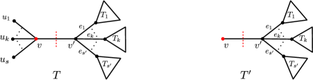
Every tree with two or more nodes contains at least two end-nodes. The following statement, illustrated in Figure 4, describes a method to produce new star-full subtrees from old ones by pruning from an end-node. Its proof is straightforward, so we omit it.
Lemma 5.2.
Let be a star-full subtree of with leaves . Fix an end-node of and assume that are the only leaves of adjacent to . Then, the convex hull is also star-full.
Definition 5.3.
A branch of a tree adjacent to a node is a connected component of
where denotes the interior of the edge .
For example, and the convex hull constructed inside the tree on the left of Figure 4 are the branches of adjacent to the node . Similarly, the branches of adjacent to are and .
Star-full subtrees of splice diagrams have a key convexity property rooted in barycentric calculus. This is the content of 5.10. The following definition plays a crucial role in its proof.
Definition 5.4.
Let be a node of and let be a set of leaves of . We define as the barycenter of the leaves in with weights determined by , that is:
| (5.2) |
In particular, for any leaf .
Remark 5.5.
Fix a node of with adjacent branches . Then, the set is linearly independent, and a direct computation gives
| (5.3) |
In particular, lies in the relative interior of the simplex , where denotes the affine convex hull inside .
Following the notation from 2.13, we write and for each pair of adjacent nodes of . Barycenters determined by splitting along the edge are closely related, as the following lemma shows:
Lemma 5.6.
Let be two adjacent nodes of , with associated sets of leaves and on each side of . Then:
-
(1)
and (which we denote by and , respectively).
-
(2)
The points and lie in the line segment .
-
(3)
, where is the order given by identifying the segment with .
Proof.
We start by showing (1). 2.6 induces the following identities:
| (5.4) |
Thus, and contribute proportional weights to and , respectively. This implies that the corresponding barycenters agree, proving (1).
Our next result shows that the image under of the vertices adjacent to a fixed node satisfy a convexity property analogous to that of 5.5:
Proposition 5.7.
Let be a node of , with adjacent vertices . Then:
-
(1)
is linearly independent;
-
(2)
.
Proof.
Both statements are clear if is only adjacent to leaves of (i.e., when is a star splice diagram), so we may assume is adjacent to some node of . Thus, up to relabeling if necessary, we suppose are leaves of and are nodes of (we set if is only adjacent to nodes).
For each , we let be the branch of adjacent to containing , and set . 5.6 (2) and the definition of barycenters ensures the existence of satisfying
| (5.6) |
with if and only if .
We start by proving (1). We fix a linear relation . Substituting (5.6) into this dependency relation yields
| (5.7) |
We claim that . Indeed, assuming this is not the case, we use (5.7) to write in terms of . Comparing this expression with (5.3) and using the linear independence of gives:
| (5.8) |
In particular, all are non-zero and have the same sign, namely the opposite sign to . Summing up the expressions (5.8) over all yields , which cannot happen due to the sign constraint on the ’s. From this it follows that .
Since , the linear independence of forces for all . Combining this with our assumption that for all , gives for all , thus confirms (1).
To finish, we discuss (2). We let be the coefficients used in (5.3) to write as a convex combination of . Substituting the value of each obtained from (5.6) in expression (5.3) yields:
| (5.9) |
The conditions for , and the definition of ensure that the right-hand side of (5.9) is a positive convex combination of , as we wanted to show. ∎
Each subtree of determines a polytope via the map :
| (5.10) |
For example, is the standard simplex . We view the next result as a key convexity property of star-full subtrees of splice diagrams.
Lemma 5.8.
Fix a star-full subtree of . For every node of , admits an expression of the form
| (5.11) |
In particular, .
Proof.
We let be the number of nodes of and proceed by induction on . The statement is vacuous for . If , then is a star tree and the result follows by 5.7 (2). For the inductive step, we let and suppose that the result holds for star-full subtrees with nodes.
We fix and we let be an end-node of . Following Figure 4, we let be the unique node of adjacent to and assume that are adjacent to . 5.7 (2) applied to gives
| (5.12) |
Using 5.2, we let be the star-full subtree of obtained by pruning from . By construction, has nodes and its leaves are . The inductive hypothesis yields the following expressions for and all other (potential) nodes of :
| (5.13) |
with and for all . Since , substituting the expression for obtained from (5.13) into (5.12) produces the desired positive convex combination for :
In turn, substituting this identity in both expressions from (5.13) gives the positive convex combination statement for all remaining nodes of . The inclusion follows by the convexity of . ∎
Corollary 5.9.
For each pair of star-full subtrees of with , we have .
Our next result is a generalization of 5.7 and it highlights a key combinatorial property shared by and all its star-full subtrees.
Proposition 5.10.
Let be a star-full subtree of . Then:
-
(1)
the weights are linearly independent;
-
(2)
is a simplex of dimension ;
-
(3)
for each node of we have .
Proof.
Item (2) is a direct consequence of (1). In turn, item (3) follows from (2) and 5.8. Thus, it remains to prove (1). We distinguish two cases, depending on the number of nodes of , denoted by .
Case 1: If , then is either a vertex, an edge of , or a star tree. If is a vertex of , then the claim holds because for any vertex of . If is a star tree, the statement agrees with 5.7 (1).
Next, assume is an edge of . We consider two scenarios. First, if joins a leaf and a node of , then the result follows immediately since and are linearly independent. On the contrary, assume joins two adjacent nodes of , say and . Pick two leaves of with and (i.e., is on the -side and is on the -side of , as seen from the edge ). 2.8 yields the following formula for the -minor of the matrix , involving the determinant of the edge , as defined in (2.1):
The last expression is positive by the edge determinant condition, so is linearly independent.
Case 2: If , we know that . We prove the result by reverse induction on . When , we have and there is nothing to prove since for all . For the inductive step, we take and label the leaves of by , . We assume that the linear independence holds for any star-full subtree with leaves. Without loss of generality we assume is a node of (one must exist since is star-full). Set .
Next, we define . By construction, is a star-full subtree of with leaves. Since is a node of , 5.8 applied to yields a positive convex combination:
| (5.14) |
To prove the linear independence for the points , we fix a potential dependency relation . Substituting (5.14) into it gives a linear dependency relation for the leaves of :
where are the leaves of adjacent to . The inductive hypothesis applied to and the positivity of each with forces for all . Thus, (1) holds. ∎
Next, we state the main result in this section, which is a natural consequence of 5.8:
Theorem 5.11.
The map from (5.1) is injective.
Proof.
We prove that the statement holds when restricted to any star-full subtree of . As in the proof of 5.8, we argue by induction on the number of nodes of . If , then is either a vertex or an edge . The statement in the first case is tautological. The result for the second one holds by construction because is linearly independent by 5.7 (1).
If , then is a star tree. Let be its unique node and be its leaves. Injectivity over is a direct consequence of the following identity:
which we prove by a direct computation. Indeed, pick with
| (5.15) |
By 5.7 (2), admits a unique expression:
Substituting this identity in (5.15) yields the following affine dependency relation for :
By 5.7 (1), we conclude that and for all . Since for all and , it follows that and . Therefore, expression (5.15) represents .
Finally, pick and assume the result holds for star-full subtrees with nodes. Let be a star-full subtree with nodes and pick an end-node of . As in Figure 4, write for the unique node of adjacent to it and for the leaves of adjacent to .
As in 5.2, let be the star-full subtree obtained by pruning from . Our inductive hypothesis ensures that is injective when restricted to . By the case we know that if . Thus, the injectivity of when restricted to will be proven if we show:
| (5.16) |
The identity follows from 5.10. Indeed, we write any on the left-hand side of (5.16) as
| (5.17) |
Recall that and by 5.9. Since as in 5.10 (3), substituting this expression into (5.17) and comparing it with the known expression for as an element of yields an affine dependency equation for . The positivity constraint on the coefficients used to write as an element of forces , and so (5.16) holds. ∎
6. Local tropicalization of splice type systems
Let be a splice diagram with leaves and let be a splice type system associated to it, as in 2.14. Fixing a total order on yields an embedding of the corresponding splice type singularity into . In this section we describe the local tropicalization of this embedded germ, following the characterization from 3.3. As a byproduct, we confirm the first half of Theorem 1.1, namely that is a complete intersection in with no irreducible components contained in any coordinate subspace.
The injectivity of the map from (5.1), discussed in Theorem 5.11, fixes a natural simplicial fan structure on the cone over in :
Definition 6.1.
Let be a splice diagram. Then, the set has a natural fan structure, with top-dimensional cones
We call it the splice fan of .
Here is the main result of this section:
Theorem 6.2.
The local tropicalization of is supported on the splice fan of .
We prove Theorem 6.2 by a double inclusion argument, first restricting our attention to the positive local tropicalization. In Subsection 6.1 we show that the positive local tropicalization of is contained in the support of the splice fan of . We prove this fact by working with simplices associated to star-full subtrees of , which were introduced in 5.1. For clarity of exposition, we break the arguments into a series of combinatorial lemmas and propositions. These results allow us to certify that the ideal generated by the -initial forms of all the series in always contains a monomial when lies in the complement of the splice fan of in .
In turn, showing that the support of the splice fan of lies in the Euclidean closure of the local tropicalization of involves the so-called balancing condition for pure-dimensional local tropicalizations. This is the subject of Subsection 6.3. An alternative proof will be given in Section 7 after proving the Newton non-degeneracy of the germ .
The fact that the positive local tropicalization of is pure-dimensional is verified in an indirect way. Our proof technique relies on the explicit computation of the boundary components of the extended tropicalization, which is done in Subsection 6.2. This establishes the first half of Theorem 1.1 discussed above (see 6.20). As a consequence, we confirm by 6.22 that the local tropicalization is the Euclidean closure of the positive one. This result together with the findings in Sections 6.1 and 6.3 complete the proof of Theorem 6.2.
Remark 6.3.
Throughout the next subsections, we adopt the following convenient notation for the admissible exponent vectors from (2.5). Given a node and a vertex of with , we define where is the unique edge adjacent to and lying in the geodesic . Similarly, given a star-full subtree of not containing , we write , where is any vertex of .
6.1. The positive local tropicalization is contained in the support of the splice fan.
In this subsection we show that the only points in contained in the positive local tropicalization are included in . We exploit the terminology and convexity results stated in Section 5.
Our first technical result will be used extensively throughout this section to determine . As the proof shows, the Hamm determinant conditions imposed on the system play a crucial role.
Lemma 6.4.
Fix a node of and let be three distinct edges of . Fix and suppose that the admissible exponent vectors from (2.5) satisfy:
| (6.1) |
Then, for some in the linear span of . If, in addition, satisfies
| (6.2) |
then for some series in the linear span of . In particular, .
Proof.
We let be the edges adjacent to and assume that , and . Using the Hamm determinant conditions, we build a basis for the linear span of where
From (6.1) we conclude that . Taking proves the first part of the statement.
For the second part, the technique yields a new basis for the linear span of with
where each is a linear combination of . Condition (6.2) then ensures that
Thus, the series satisfies the required properties. In particular, the ideal contains the monomial and so by definition. ∎
Next, we state the main theorem in this subsection, which yields one of the required inclusions in Theorem 6.2 when choosing . More precisely:
Theorem 6.5.
For every star-full subtree of , we have .
Proof.
Recall from (5.10) that is the convex hull of the set of leaves of , viewed in via the map . We proceed by induction on the number of nodes of , which we denote by . If , then is either a vertex or an edge of , and . For the inductive step, assume and pick a node of . Let be the branches of adjacent to , as in 5.3. We use the point to perform a stellar subdivision of , giving a decomposition , where
| (6.3) |
By 5.8, is a simplex of dimension . 6.7 below shows that lies in the boundary of . In turn, 6.10 below ensures that
where is the unique branch of adjacent to that contains the leaf , and denotes the convex hull in of . Combining this fact with the inductive hypothesis applied to all star-full subtrees of with gives
| (6.4) |
As a natural consequence of this result, we deduce one of the two inclusions required to confirm Theorem 6.2:
Corollary 6.6.
The positive local tropicalization of is contained in the support of the splice fan of .
In the remainder of this subsection, we discuss the two key propositions used in the proof of Theorem 6.5. We start by showing that the relative interior of any of the top-dimensional simplices from (6.3) obtained from the stellar subdivision of induced by a node of does not meet . 6.4 plays a central role. The task is purely combinatorial and the difficulty lies in how to select the triple of admissible exponent vectors required by the lemma. Throughout, we make use of branches of subtrees, which were introduced in 5.3.
Proposition 6.7.
Let be a star-full subtree of and . Consider the simplex defined by (6.3). Then, its relative interior is disjoint from .
Proof.
Let be the unique node of adjacent to , and denote by the branches of adjacent to . We assume that and fix any . Since is a simplex, we can write uniquely as
| (6.5) |
and for all .
In what follows we analyze the -initial forms of the series from for and use 6.4 to confirm that . To this end, we compare the -weights of and of the remaining monomials in , for each . We treat the monomials appearing in and separately.
6.8 discusses the monomials in and confirms that the required condition (6.2) of 6.4 holds for . In turn, 6.9 verifies that we can find two edges of adjacent to satisfying the inequalities (6.1) for . Therefore, 6.4 applied to the node confirms that is the -initial form of a series in the linear span of . Thus, as we wanted to show. ∎
In the next two lemmas we place ourselves in the setting of 6.7. In particular, we use the notations introduced in its proof.
Lemma 6.8.
Let be a weight vector satisfying condition (6.5). Then, for each and each monomial appearing in we have
| (6.6) |
Proof.
First, we compare the -weights of and all the monomials appearing in . We do so by looking at the weight contributed by each summand of in the decomposition (6.5). 2.18 and conditions (2.10) ensure that
| (6.7) |
In turn, to compare the -weights of the monomials and , we notice that the only summands of contributing a positive weight to are the ones coming from those that are nodes in . Again, 2.18 and the conditions on listed in (2.10) confirm that
Combining this inequality with the positivity of the coefficients yields the inequality
| (6.8) |
Furthermore, the leftmost inequality is strict if the set is non-empty.
Lemma 6.9.
Let be a weight vector verifying condition (6.5). Then, there exist two different edges adjacent to the node of satisfying
Proof.
We use the notation introduced in 6.3. It is enough to find two different branches and of adjacent to with , and verifying
| (6.9) |
Our choice will depend on the nature of . If we pick any pair of distinct indices . On the contrary, if we take to be the unique branch of adjacent to containing , and let be any other branch of adjacent to not containing with . After relabeling, we may assume that and .
In the remainder, we confirm that these two branches satisfy the inequalities in (6.9) by analyzing the contributions of each summand of in the decomposition (6.5) to the total weight of each of the three relevant monomials. We follow the same reasoning as in the proof of 6.8. 2.18 is again central to our computations.
We start with the contribution of . The lemma confirms that
| (6.10) |
To analyze the -weight of the three monomials, we recall from the proof of 6.8 that we need only consider the contributions of those vertices that are nodes of . Indeed, we have
| (6.11) |
This expression agrees with the value of when even if is the empty-set.
If , 2.18 confirms that
| (6.12) |
The inequality is strict even if the set is empty. Indeed, the fact that the tree is star-full ensures that when , any variable appearing in will be indexed by an element in . Therefore, the total -weight of is positive no matter the choice of admissible exponent .
Our next result is central to the inductive step in the proof of Theorem 6.5. As with the previous two lemmas, the proof is combinatorial and the difficulty lies in how to select the triple of admissible exponent vectors required by 6.4 in a way that is compatible with a given input proper face of .
Proposition 6.10.
Let be a star-full subtree of , and let be a node of . Denote by the branches of adjacent to . Let be a proper subset of which is not included in any , and set
| (6.13) |
Then, is a simplex of dimension and its relative interior is disjoint from .
Proof.
By 5.8, we have . In addition, 5.10 (2) and (3) imply that is a simplex of the expected dimension. It remains to show that . For each , we set
| (6.14) |
By definition, we have if . Moreover, each is a simplicial cone of dimension . Our assumptions on and a suitable relabeling of the branches (if necessary) ensure the existence of some with for all and for all .
We argue by contradiction and pick . Since is a simplex and belongs to its relative interior, we may write as
| (6.15) |
6.11 below implies that for all . Since , it follows that .
Next, we use 6.4 to confirm that is the -initial form of a series in the linear span of , which contradicts our assumption . We use the admissible exponents , and .
First, the star-full property of combined with the condition that for all ensures that
| (6.16) | ||||
These identities follow directly from 2.18. In turn, the same arguments employed in the proof of 6.9, together with the equalities and give
| (6.17) |
Expressions (6.16) and (6.17) combined yield and . Thus, the first condition required by 6.4 is satisfied.
To finish, we must compare the -weight of with that of any exponent in the support of a fixed series . For each we write with for all . Then, the defining properties (2.10) of and the reasoning followed in the proof of 6.8 imply that
| (6.18) |
Note that the right-most inequality for is strict whenever .
Lemma 6.11.
Proof.
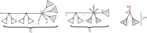
We argue by contradiction and assume , so in particular . We break the argument into four combinatorial claims, guided by Figure 5. The left-most picture informs the discussion for Claims 1 and 2. The central picture refers to 3, and the right-most picture illustrates 4. Throughout, we fix and write as in (6.15), where we write each as for each , with for all .
First, we pick furthest away from in the geodesic metric on (see 2.2). Let be the unique node of adjacent to . The condition ensures that . The maximality condition satisfied by restricts the nature of the node . More precisely:
Claim 1.
The node is an end-node of .
Proof.
We consider all branches of adjacent to and containing neither nor . Our goal is to show that for all . We argue by contradiction.
Assume that is such that . Then, by the maximality of the distance between and , we have . We consider the series of for , and the admissible exponent vectors at associated to , and . We claim that the weight satisfies the inequalities
| (6.19) |
for each in the support of some . This cannot happen by 6.4, since .
To prove the inequalities (6.19), we analyze the contributions of each summand of in the decomposition (6.15) to the total -weight of each admissible monomial, as we did in the proofs of Lemmas 6.8 and 6.9. Here, the node appearing in those lemmas is replaced by the node . As usual, 2.18 is central to our arguments. The contribution of each weight vector for to the total weight of comes from elements in .
We start by verifying the left-most inequality in (6.19). Since is a node of , 2.18 ensures that:
| (6.20) |
In turn, for each with , the weight satisfies
| (6.21) |
On the contrary, if , the condition ensures that . Indeed, separating the -weight of into the contributions of three groups of elements from we have
| (6.22) |
Notice that whenever and for .
Similarly, the -weight of can be determined by separating the elements of into two types:
| (6.23) |
Comparing expressions (6.22) and (6.23), the positivity of all the coefficients implies the inequality if the set is non-empty. In turn, if this last set is empty, the fact that is star-full ensures that all variables featuring in the admissible monomial are indexed by elements of . Therefore, the last summand in (6.22) is strictly positive. Thus, the comparison of the same two expressions gives in this situation as well.
By adding up the strict inequality and the equalities from (6.21) for each , we obtain:
Combining this inequality with the decomposition (6.15), the equality from (6.20) yields the left-most strict inequality in (6.19).
Next, we confirm the central inequality in (6.19). By (6.20) and the positivity of , it is enough to check that for all . Indeed, 2.18 yields:
| (6.24) |
since all coefficients are positive, for each and if .
To finish, we must certify the right-most inequality in (6.19). We use the same reasoning as in 6.8. The properties defining the series combined with the star-full condition of , the inclusion and the expressions (6.20), (6.21) and (6.23) imply that for each monomial appearing in a fixed we have the inequalities
The inequality then confirms the validity of the right-most inequality in (6.19).
Claim 2.
We have . In particular, none of the leaves of adjacent to can lie in .
Proof.
Since is an end-node by 1, any branch of emanating from and not containing is a singleton. The statement follows by the same line of reasoning as 1, working with the exponents , and , where is any of the remaining branches of adjacent to . Indeed, if , the inequalities in (6.19) will remain valid, and this will contradict .
As a consequence of 2 we conclude that is part of a branch of which avoids and has at least one node. Let be a maximal branch of with this property and furthest away from . We claim that . To prove this, we argue by contradicting the maximality of . We let be the node of adjacent to and be the node of adjacent to , as seen in the center of Figure 5. Note that since because is non-empty.
Next, we analyze the intersections between and the leaves of all relevant branches of adjacent to . We treat two cases, depending on the size of each such branch, starting with singleton branches:
Claim 3.
None of the leaves of adjacent to belongs to .
Proof.
Claim 4.
Given a non-singleton branch of adjacent to and with , we have .
Proof.
First, we show that . We argue by contradiction and consider the series of determined by the node . Replacing the roles of , and in (6.19) by , and , respectively, the same proof technique from 1 yields
for each in the support of any fixed . 6.4 then shows that , contradicting our original assumption on . From here it follows that .
Next, we pick some leaf . Following the reasoning of Claims 1 and 2, we build a maximal branch of not meeting . If this branch would be a maximal branch of avoiding and properly contained in . Furthermore, following the notation of the right-most picture in Figure 5, it would be contained in one of the branches for . As a result, the distance between and this branch would be strictly larger than , contradicting the maximality choice of . Thus, we conclude that , as we wanted to show.
6.2. Boundary components of the extended tropicalization
In this subsection, we characterize the boundary strata of the extended tropicalization of the germ defined by (see 3.7). These strata are determined by the positive local tropicalization of the intersection of with each coordinate subspace of . This will serve two purposes. First, it will show by combinatorial methods that is a two-dimensional complete intersection with no boundary components (that is, without irreducible components contained in some coordinate hyperplane). Second, it will help us prove the reverse inclusion to the one in Theorem 6.5. The latter is the subject of Subsection 6.3 (see Theorem 6.23).
We start by setting up notation. Throughout, we write and fix a positive-dimensional proper face of . Since by choosing the basis from Section 2, we define
| (6.26) |
We let be the dimension of and consider the natural projection of vector spaces
| (6.27) |
By abuse of notation, whenever , we identify with its image in under .
Definition 6.12.
Given a series , we let be the series obtained from by setting all with to be zero. We view as a series in the variables in . We call it the -truncation of .
Definition 6.13.
We let be the intersection of the germ defined by with the dense torus in the -dimensional coordinate subspace of associated to . This new germ is defined by the vanishing of the -truncations of all series in . The positive local tropicalization of with respect to is defined as the positive local tropicalization of in . Following [49, Section 12], we denote it by .
Our first result generalizes 6.4, when some, but not all, admissible monomials at a fixed node of have trivial -truncations. It will simplify the computation of for each proper face of .
Lemma 6.14.
Fix a positive-dimensional proper face of , a node of and some . Assume that some -truncated series in is not identically zero and that one of two conditions holds:
-
(1)
the system involves at most admissible monomials and there exists an edge adjacent to with satisfying for each in the support of some ; or
-
(2)
the system involves exactly monomials, and we have two distinct edges , of with such that and for each in the support of some .
Then, is the -initial form of a series in the linear span of and .
Proof.
Recall from (2.9) that for each node of and each . Our assumptions on and the weight vector ensure both that the -truncation of is non-zero and that the -initial form of agrees with that of .
The proof follows the same reasoning as that of 6.4, considering the truncations of a new basis obtained by suitable linear combinations of the original series and ordering the edges adjacent to in a convenient way. Writing each element in the new basis as in the spirit of (2.9), the Hamm determinant conditions on the original splice system allow us to choose a special form for the polynomials . Indeed, their coefficient matrix has the block form , where represents a column vector in . By construction, the new tails will satisfy conditions (1), respectively (2), if and only if the old tails did.
If condition (1) holds, we pick any two edges with and order the edges adjacent to so that , and . In this situation, the statement follows by our assumptions on the basis , combined with 2.18. Indeed, we have
Similarly, if condition (2) holds, we pick to be the unique edge with . Indeed, is the single monomial of the polynomials that drops when taking their -truncations. We set and fix and . As in the previous case, we have . ∎
Here is the main result of this section:
Theorem 6.15.
Let be a positive-dimensional proper face of with . Let be the unique node of adjacent to . Then:
-
(1)
If , then .
-
(2)
If , then .
Proof.
We fix . Since is included in , we can determine the positive tropicalization by its intersection with the standard simplex . We do this by following the proof strategy of Theorem 6.5. Since the vector lies in , we set
| (6.28) |
and perform a stellar subdivision of this standard simplex using .
If , 6.16 below ensures that every positive-dimensional simplex of the stellar subdivision that meets satisfies . The subdivision has only one zero-dimensional simplex, namely , so item (1) holds. In turn, when , the same proposition ensures the intersection is empty even if is a point. This forces , as stated in item (2). ∎
Our next result is an adaptation of 6.10, needed to rule out points of the extended tropicalization in a given simplex . It is central to proving Theorem 6.15.
Proposition 6.16.
Let , and be as in Theorem 6.15 and be as in (6.26). Fix a proper subset of . Let be as in (6.28) and set , where . If , then
| (6.29) |
Proof.
We follow the proof strategy of 6.10 for but now incorporating the set into the arguments. We let be the branches of adjacent to , with . Given , we set
| (6.30) |
If , we declare . Since , upon relabeling the branches if necessary, there exists a unique with for all , and for .
We argue by contradiction and pick . Since is a simplex and , we have
| (6.31) |
In particular, we know that if and only if .
6.17 below ensures that for all . Since , we conclude that:
| (6.32) |
In particular, we see that , so the -truncation of is non-zero.
By the Hamm conditions, the admissible monomial must feature in some . Therefore, the -truncated series are not all identically zero. In turn, since and , we conclude that its -truncation is zero. Thus, the system of -truncations involves at most admissible monomials.
The proposition follows from our next claim, which contradicts our assumption that .
Claim 1.
The monomial is the -initial form of a series in the linear span of .
The statement of this claim matches the conclusion of 6.14. Recall that our earlier discussion confirmed that the -truncations of are not all zero, and there are two options for the number of monomials featured in these -truncations. We prove the claim via a case-by-case analysis, each one matching one of the two possible scenarios portrayed in the lemma.
First, we assume that the system of -truncations involves exactly monomials. In particular, , so no variable appearing in can be indexed by an element of . Since , we conclude that and .
Next, we confirm that the hypotheses of 6.14 (2) hold for the weight vector and the edges and giving rise to the admissible exponents and , respectively. Notice that our earlier discussion ensures that these two vectors lie outside . To check the required inequalities between the -weights of these two admissible monomials and of any monomial in the support of some , we compare the contribution of each summand of featured in (6.31) to the total -weight of each monomial. This was the same method used in the proofs of Lemmas 6.8 and 6.9.
First, we focus on . 2.18 and the conditions (2.10) on imply that
| (6.33) |
In turn, our earlier discussion and the inequality seen in (6.32) imply the following relations among the -weights:
| (6.34) |
where is any monomial in the support of surviving the -truncation. Combining the positivity of with expressions (6.33) and (6.34) confirms the validity of the conditions required in 6.14 (2).
To finish proving the claim, we must analyze the case when the -truncated system has at most admissible monomials. In this case, we consider the edge and certify that the hypotheses imposed in 6.14 (1) hold. This is done by checking that the inequalities in (6.33) and (6.34) involving and remain valid in this new setting. ∎
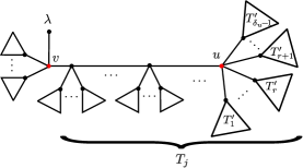
Our next result is analogous to 6.11. We prove it by using the same techniques.
Lemma 6.17.
Fix , and as in (6.30). If , then the set is either empty or it equals .
Proof.
We use the notation established in the proof of 6.16 and pick . We decompose as in (6.31). We argue by contradiction, assuming that .
First, note that we can find a branch of contained in with . For example, any leaf of not in will produce such a branch. Since is finite, we can choose the branch to be maximal with respect to the condition and furthest away from in the geodesic metric on . Let be the unique node of adjacent to . Since , we know that .
Assume that there are branches adjacent to with this maximality property, and denote them by as in Figure 6. We let be the remaining branches of adjacent to and not containing . The maximality of both and combined with the condition implies that and for each . Indeed, if the latter were not the case, we could find a branch of inside with the same properties as , but further away from .
The construction of ensures that . Therefore, the collection is not identically zero. Our original assumption that will be contradicted by the following assertion:
Claim 2.
The admissible monomial is the -initial form of a series in the linear span of .
We prove our claim by analyzing three cases (in decreasing order of difficulty), depending on whether the number of admissible monomials in the -truncation of the collection is exactly , at most , or exactly . The first case will make use of 6.4, whereas we will invoke 6.14 to establish the other two.
Case 1: We assume that the number of admissible monomials at remaining after -truncation is . By the Hamm conditions, this forces for each . After replacing each with its -truncation, we are in the setting of 6.4, where we view by adding zeros as complementary coordinates. In this situation, the condition and the defining properties of ensure that
| (6.35) |
for each appearing in . The aforementioned lemma then implies the validity of our claim.
To prove the inequalities in (6.35), we proceed by comparing the contributions of each summand of in the decomposition (6.31) to the weight of each monomial. 2.18 and (2.10) ensure that
| (6.36) |
In turn, for each with , the fact that contains no node of gives
| (6.37) |
Finally, since , and the admissible monomial has no variable indexed by an element in , we see that
| (6.38) |
Expressions (6.36), (6.37) and (6.38), combined with the positivity of confirm (6.35).
Case 2: Assume that the -truncated series involve at most admissible monomials. In this situation, the claim follows by 6.14 (1) since the inequalities involving and in (6.35) remain valid in this scenario.
Case 3: Suppose that the -truncations of the collection involve exactly admissible monomials. If so, up to relabeling of we may assume that exactly one of the admissible monomials with exponent or vanishes under -truncation. The inequalities in (6.35) involving , and the aforementioned surviving admissible exponent remain valid. Thus, the hypotheses required by 6.14 (2) hold, hence confirming the claim. ∎
Theorem 6.15 has the following two important consequences:
Corollary 6.18.
The intersection of the germ defined by the system with any coordinate subspace of of codimension at least two is just the origin.
Proof.
Assume the contrary and let be a coordinate subspace of of maximal codimension such that . Consider the face of associated to and let be the intersection of with the dense torus of . The maximality condition on implies that . Since by 3.12 (1), we conclude that .
Since the dimension of agrees with the codimension of in , our hypothesis implies that . Therefore, we have by Theorem 6.15 (2). This contradicts our earlier observation. ∎
Corollary 6.19.
The germ defined by the system intersects each coordinate hyperplane along a germ of a curve. All its irreducible components meet the dense torus of the corresponding hyperplane.
Proof.
We fix a coordinate hyperplane and let be the cone generated by in . Counting the number of equations defining in , we see that by Krull’s principal ideal theorem. By construction, . Since any face of properly containing satisfies by 6.18, it follows that no component of lies in the toric boundary of . Furthermore, 3.12 (1) implies that . Since Theorem 6.15 (1) ensures that , we conclude that . ∎
In turn, the last corollary has two consequences. First, it confirms that the germ defined by is a complete intersection, and second, it shows that equality must hold in Theorem 6.15 (1).
Corollary 6.20.
The germ defined by the system is a two-dimensional complete intersection. Each of its irreducible components meets the dense torus non-trivially in dimension two.
Note that this result allows a priori for the germ to have several irreducible components. We will see in 7.13 that is in fact irreducible.
Corollary 6.21.
Let be a leaf of and let be the unique node of adjacent to it. If , then .
Proof.
The result follows by combining Theorem 6.15 (1), 6.19, and the equality between the dimensions of and stated in 3.12 (1). ∎
Our last result in this subsection is a special case of 3.10. It will be used in the next subsection.
Corollary 6.22.
The local tropicalization of the germ defined by the splice type system is the Euclidean closure of in .
6.3. The support of the splice fan is contained in the local tropicalization.
In this subsection, we prove the remaining inclusion in Theorem 6.2. Our arguments are purely combinatorial, and rely on the balancing condition for pure-dimensional local tropicalizations (see Theorem 3.20 and 3.21). 6.20 confirms that such condition holds for the positive tropicalization of the germ defined by . Furthermore, the proofs in this section imply that no proper two-dimensional subset of is balanced.
We start by stating the main result in this section. Its proof will be broken into several lemmas and propositions for clarity of exposition.
Theorem 6.23.
For every splice diagram , we have in .
Proof.
By 6.24 below we know that is a 1-dimensional polyhedral complex and for some node of . We claim that, in fact, for each node .
We prove this claim by induction on the distance between and (recall that is connected). If there is nothing to show. For the inductive step, pick a node with and assume that the claim holds for each node of with . Let be the unique node of adjacent to . Then, by our inductive hypothesis. 6.26 below and 6.22 yield:
The desired inclusion follows by combining 6.26 with the identity
Our first lemma ensures that the image of some node of lies in the positive tropicalization of :
Lemma 6.24.
The intersection is a 1-dimensional polyhedral complex. Furthermore, there exists a node of with .
Proof.
Our next lemma is central to the proof of both Theorem 6.23 and 6.24. It describes the possible intersections between the local tropicalization of the ideal and the edges of embedded in via the map . The balancing condition for positive local tropicalizations plays a prominent role.
Lemma 6.25.
Let be two adjacent vertices of . If intersects non-trivially, then .
Proof.
It suffices to show that . We argue by contradiction and fix a point . Let be the affine map such that and . There exists a unique such that . Since is closed in , we can find a pair satisfying and such that the open segment avoids . Furthermore, we pick to be the maximal open interval in containing with this property. A contradiction will arise naturally if we prove that and .
By symmetry, it suffices to show that . We argue by contradiction, and assume , so by construction. The maximality of combined with 6.22 ensures that . Recall from 6.6 that . Since is an injection by Theorem 5.11, any neighborhood of in lies in the relative interior of the two-dimensional cone . In turn, since is two-dimensional, and avoids , it follows that is not balanced at when . Indeed, the balancing condition (see Theorem 3.20) at involves a single non-zero vector, namely, the image of in the lattice , and a non-zero scalar. Therefore, we must have . ∎
Our next result plays a prominent role in the induction arguments used to prove Theorem 6.23. Once again, as in the proof of 6.25, the balancing condition for local tropicalizations is crucial in our reasoning.
Proposition 6.26.
Let be a node of with . Then, .
Proof.
After refinement if necessary, we may assume that is a ray of . In order to exploit the balancing condition, we use analogous notation to that of 3.18, simplified slightly by the fact that is 2-dimensional.
Given a vertex of adjacent to , we consider the 1-dimensional saturated lattice
Fix a vector whose natural projection to generates this lattice. In particular, we can write uniquely as
| (6.39) |
for some and with .
We let be the vertices of adjacent to . The balancing condition for at combined with Theorem 6.5 ensures the existence of non-negative integers (i.e., the tropical multiplicities of 3.17) satisfying:
| (6.40) |
Moreover, by 3.17, intersects non-trivially in a neighborhood of if and only if .
Since is pure of dimension two and , we know that for some . We claim that, furthermore, all are positive integers. The inclusion follows by combining this statement with 6.25.
To prove our claim, we consider the following linear equation in that is equivalent to (6.40):
| (6.41) |
First, we argue that this system admits a unique solution for all . Uniqueness follows directly since for all and the set is linearly independent by 5.10 (1).
7. Splice type singularities are Newton non-degenerate
In this section we discuss the Newton non-degeneracy of splice type systems (see Theorem 7.3), following the original framework introduced by Khovanskii (see 4.2). This property only involves the initial forms of the generators of the system , as opposed to the initial ideals of the ideal generated by the elements of the system . In turn, Theorem A.1 ensures the -initial forms of generate the -initial ideal of , for each rational weight vector in the positive local tropicalization of , thus giving an alternative proof of Theorem 6.23. Furthermore, Newton non-degeneracy implies that condition (3) of 3.12 holds for every cell in , thus showing that the splice fan of is a standard tropicalizing fan for the germ defined by the system , in the sense of 3.14. This is the content of 7.10. In turn, 7.14 gives an alternative proof of a recent theorem of de Felipe, González Pérez and Mourtada [11], which resolves any germ of a reduced plane curve by one toric morphism after a reembedding in a higher dimensional complex affine space. The section concludes with an open question regarding embedding dimension of splice type surface singularities preserving the Newton non-degeneracy property (see 7.16).
Our first result is a direct consequence of 2.18 and (2.10). It allows us to determine the -initial form of each series in the system for each node of . This computation is central to all arguments in this section:
Proposition 7.1.
For each pair of nodes in , and each , we have:
where is the unique edge adjacent to with .
The second formula, for the case where , means that we remove from the term associated to the edge starting from in the direction of .
Remark 7.2.
Recall from 2.19 that rooted splice diagrams with leaves (including the root ) give rise to end-curves in . Consider a fixed strict splice type system associated to giving rise to this curve and let be the unique node of adjacent to . In view of 7.1, the curve is defined by the vanishing set of and the -initial forms of the polynomials in the system , viewed in .
Next, we set up notation that we will use throughout this section. For each weight vector we define:
| (7.1) |
and let be the subscheme of defined by .
Next, we state the main result of this section. The rest of the section is devoted to its proof.
Theorem 7.3.
The splice type system is a Newton non-degenerate complete intersection system.
Proof.
We certify the two conditions from 4.2 starting with the regularity of the sequence defined by . This property follows by 7.4 and Theorem A.1. Indeed, since the weight vector associated to any node of lies in , and is a complete intersection of dimension two with defining ideal by the lemma, we conclude that the generators of form a regular sequence in . In turn, the theorem confirms that the series form a regular sequence in .
Recall from 3.3 that is the empty-set whenever . Thus, it suffices to certify the linear independence condition of the differentials of when . In turn, by Theorem 6.2 it is enough to restrict our analysis to vectors .
Since the generators of form a regular sequence in by 7.7, 4.4 simplifies our task: we need only verify that is smooth for each such . We analyze three cases, depending on the nature of the unique cell of containing in its relative interior. Each case matches the settings of Lemmas 7.4, 7.5 and 7.6 below.
First, we pick a node of and consider the weight vector . By 7.4, the components of the scheme are Pham-Brieskorn-Hamm singularities, and they can only meet at coordinate subspaces of . Furthermore, the Hamm conditions ensure that these germs are smooth away from the origin. This fact confirms the smoothness of .
Next, we consider a weight vector , were is a leaf of and is a node of adjacent to . Then, by 7.5, is a cylinder over an end-curve associated to the rooted diagram . By Theorem 2.20, such curves are smooth away from the origin. This confirms that is smooth in this case as well.
Finally, we fix a weight vector where are adjacent nodes of . Then, 7.6 confirms that the scheme is the product of two end-curves and associated to two splice subdiagrams of rooted at and , respectively. More precisely, we have and in the notation of 2.13. By Theorem 2.20, these curves are smooth in the corresponding ambient tori, so is smooth. This concludes our proof. ∎
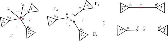
The next three lemmas characterize the ideal associated to points in the relative interior of each cell in the piecewise-linearly embedded tree .
Lemma 7.4.
Let be a node of and let . Let be the star of at , viewed as a splice diagram with inherited weights around . Then:
-
(1)
;
-
(2)
is a complete intersection of dimension two;
-
(3)
has no irreducible component contained in a coordinate hyperplane of , so is monomial-free;
-
(4)
all components of are obtained as images of torus-translated monomial maps and their preimages lie in Pham-Brieskorn-Hamm complete intersections in determined by ;
-
(5)
the intersection of any two distinct components of lies outside of .
Proof.
Item (1) follows from the identity for all and , seen in 7.1. To prove the remaining items, we let be the number of nodes of adjacent to and be the branches of adjacent to containing these nodes, as seen in Figure 7. Set and express as the sum of the following ideals:
Note that the generators of each with lie in . In particular, no variable with adjacent to appears in them. We call these leaves , with .
To simplify notation, we write . We start by characterizing the components of . Each ideal with defines an end-curve determined by the splice diagram rooted at , as seen in the center of Figure 7. In turn, Theorem 2.20 ensures that each of the (-many) components of admits a (torus-translated) monomial parameterization of the form
| (7.2) |
with for all . Thus, each component of can be parameterized using by combining these (torus-translated) monomial maps.
Substituting the expressions from (7.2) for the chosen component of each into the generators of shows that the closure of each component of can be parameterized using a component of a splice type singularity defined by the diagram . Note that the Hamm determinant conditions at arising from agree with those determined by the generators of up to multiplying the columns corresponding to the branches , by non-zero constants. Therefore, each component of is the image of a (torus-translated) monomial map from restricted to a Pham-Brieskorn-Hamm complete intersection defined by . In particular, no component of lies in a coordinate subspace of , so is monomial-free. This proves both (3) and (4).
Since is equidimensional of dimension two and it is defined by polynomial equations, it is a complete intersection. This proves (2). It remains to address (5) when is not irreducible.
To determine the intersection of two distinct components (say, and ) of we exploit the parameterization described earlier. Let be the collection of indices for which the projections of and to disagree. If , then the two components are parameterized using the same Pham-Brieskorn-Hamm system of equations associated to and the same (torus-translated) monomial map. This cannot happen since such germs are irreducible and .
Next, assume . In this setting, the projection of to for each lies in the intersection of two components of the end-curve , which can only be the origin of by Theorem 2.20. This means that lies in the coordinate subspace of defined by the vanishing of all with . This concludes our proof. ∎
Lemma 7.5.
Let be a node of adjacent to a leaf and pick . Then, is a cylinder over a monomial curve in with many components and is monomial-free.
Proof.
We prove that defines the cylinder over the end-curve associated to the rooted splice diagram . A simple inspection shows that for all nodes of and each , the initial form agrees with the corresponding polynomial defining (see 2.19). Indeed, if we write as
| (7.3) |
then the defining properties of ensure that for all . In turn, combining this fact with 2.18 and 7.1 yields
Furthermore, equality holds if and only if . Thus, is obtained from by dropping the admissible monomial at pointing towards . In particular, these initial forms do not involve .
The above discussion shows that defines . The general point of this curve lies in by Theorem 2.20, so is monomial-free. In turn, the same result confirms that defines a reduced complete intersection, smooth outside the origin, and with many irreducible components. Since is obtained from by base change to , and both ideals admit a common generating set, the result follows. ∎
Given two adjacent nodes and of , we let be the branch of adjacent to containing . Similarly, we let be the branch of adjacent to and containing . Our final lemma is analogous to 7.5:
Lemma 7.6.
Let and be two adjacent nodes of and pick . Then, is isomorphic to a product of two monomial curves in . Furthermore, the number of irreducible components of equals and is monomial-free.
Proof.
We write with and follow the same proof-strategy as in 7.5. By Theorem 5.11, we can find a unique with (see the rightmost picture in Figure 7).
The conditions on together with 7.1 guarantee that for each node in , . Furthermore, each form is obtained from by dropping the admissible monomial at pointing towards . This observation and the symmetry between and determine a partition of the generating set of , where each initial form for any node of (respectively, in ) only involves the leaves of (respectively, of ). Thus, each set determines an end-curve for the diagrams and , respectively, both rooted at .
By construction, defines the product of these two monomial curves. Since each of them is a complete intersection in their respective ambient spaces, the same is true for . The number of components is determined by Theorem 2.20. Since meets , we conclude that is monomial-free. ∎
The next result is a direct consequence of Theorem A.1 and the previous three lemmas. It gives an alternative proof of Theorem 6.23 since for any in , these lemmas confirm that is monomial-free.
Corollary 7.7.
For any strictly positive vector in the splice fan of , we have , where is the ideal generated by the splice type system .
Proof.
By construction, we have for each . In addition, Lemmas 7.4, 7.5 and 7.6 imply that the generators of form a regular sequence in the ring of convergent power series near the origin. Thus, Theorem A.1 implies that as ideals of for each . Finally, since these ideals are constant when we consider all rational points in the relative interior of any fixed edge of , 7.8 below confirms that the same must be true for all points in these open segments. ∎
Lemma 7.8.
Fix an edge of . If is constant for all , the same is true for all .
Proof.
We set , , and fix a weight vector . We wish to show that for all . We prove this equality by double-inclusion.
The inclusion is a direct consequence of the following claim:
Claim 3.
For each , we have .
Proof.
Throughout our reasoning, we need the following auxiliary fact. By [28, Lemma 2.4.6], given and in , there exists with
| (7.4) |
for all and for each . Restricting further the value of to require that whenever , extends the validity of (7.4) to convergent power series .
Since by construction, the initial form is a polynomial. Its Newton fan is rational and complete, and we get an induced rational fan (denoted by ) on the cone by common refinement. Thus, cannot be a ray of (the vector is not rational), so it lies in a 2-dimensional cone of . By construction, . Picking any , our earlier discussion ensures the existence of with
Since the set contains a point in , we conclude that .
For the reverse inclusion, we argue as follows. Direct calculations used in the proofs of Lemmas 7.5 and 7.6 confirm the identities
In turn, Theorem A.1 ensures that this collection generates . Thus, , as desired. ∎
Remark 7.9.
The geometric information collected in Lemmas 7.5 and 7.6 combined with 7.7 determines the tropical multiplicities of . Using 2.7 and 3.17, we have:
-
(1)
if for a node of , then has multiplicity
-
(2)
if for two adjacent nodes and of , then has multiplicity
This information completes the characterization of as a tropical object, i.e., as a weighted balanced polyhedral fan. We use this data in Section 8 when discussing how to recover from its splice fan.
Corollary 7.10.
The splice fan of is a standard tropicalizing fan for the germ defined by , in the sense of 3.14.
Next, we show how we can use their local tropicalizations to recover some known facts about splice type systems and their associated end-curves from [38, 39]. Our first statement discusses the intersections of the initial degenerations of the germ defined by will suitable codimension-2 coordinate subspaces of :
Lemma 7.11.
Let be a vector in which lies in the embedded splice diagram , and let and be two leaves of in different branches of adjacent to . Then, the system
| (7.5) |
has as its only solution.
Proof.
If is the (normalized) weight vector corresponding to a node of , this statement is proved as part of [38, Theorem 2.6], more precisely, on [38, page 710]. For any point in , the claim follows by similar arguments, but for the reader’s convenience, we give a complete proof that includes the node case. Our reasoning is guided by Figure 7, and it is based on the techniques discussed in the proofs of Lemmas 7.4, 7.5 and 7.6.
By Theorem 5.11, we can find a unique point in with . As in the figure, we write if is a node of . Otherwise, is in the relative interior of a unique edge , where is a node of but is allowed to be a leaf of . The proofs of the three aforementioned lemmas ensure that for all nodes in and . Thus, to prove the statement, we may assume that for all .
By abuse of notation, we think of the point as a node of (potentially, of valency two). We assume is adjacent to nodes and leaves of , with . We let be the branches of adjacent to . We assume contain nodes of , whereas the remaining branches are singletons. We view the single vertex of a singleton branch as a leaf of this branch.
Using , we build a collection of rooted splice diagrams rooted at . Each is obtained as the convex hull . In particular, if (as in the right of the figure), then is the number of nodes of among . We assume that whenever .
Throughout, we consider the ideals
| (7.6) |
The generators of are among the series of the system (7.5) per our assumption on the tails . Since is not a node of , 2.18 confirms that is generated by polynomials in . Viewed in this ring, the ideal defines an end-curve in associated to the rooted diagram (see 7.2).
Next, we consider a solution of the system (7.5). Our assertion that is the origin will follow by combining the next two claims:
Claim A 1.
Fix and assume that for some leaf of . Then, for all leaves of .
Proof.
If , then and the statement is tautological. On the contrary, if , then the projection of to lies in the end-curve . Since , Theorem 2.20 guarantees that the projection of is the origin of , as we wanted.
Claim B 1.
Assume that all coordinates of indexed by two different branches (say, and ) adjacent to vanish. Then, the same is true for each remaining branch.
Proof.
If , there is nothing to show. On the contrary, if , we consider the splice type polynomials for . By 7.1, for each .
Using the Hamm conditions, we may assume that each involves exactly three admissible monomials, two of which are and . The third one equals . Since the first two monomials vanish along by construction, we deduce that the same is true for the remaining monomial in . Thus, for each of the remaining branches adjacent to we have for some leaf in . Claim A ensures that the same is true for all leaves of . This concludes our proof.
To finish our proof, it is enough to notice that the hypothesis of Claim B holds by combining Claim A with the fact that the leaves and belong to distinct branches of adjacent to . ∎
Our second statement gives a stronger version of 2.21:
Corollary 7.12.
Assume that the conditions of 7.11 hold and consider the map obtained from the collection , ordered appropriately. Then, the restriction of this map to the codimension- subspace of is surjective.
Proof.
By 7.11, we see that the fiber of the restriction of to over the origin of is -dimensional. By upper semicontinuity of fiber dimensions, the generic fiber of is also -dimensional. Since , the map is dominant.
Since is defined by weighted homogeneous functions, it admits a projectivization as a map between weighted projective spaces. But a dominant projective map must be surjective. Thus, as an affine map, is surjective as well. ∎
Next, we recover Theorem 2.16 (originally due to Neumann and Wahl) by combining 6.18 with the following result:
Corollary 7.13.
The singularity defined by the splice type system is isolated. In particular, it is also irreducible.
Proof.
Let be the germ defined by . By 6.20, we know that is dense in . Since is a Newton non-degenerate complete intersection system by Theorem 7.3, we conclude that admits an embedded toric resolution (see, e.g., Khovanskii [23, Section 2.7] and Oka [41, Chapter III, Theorem (3.4)]). In particular, for a suitable subdivision of the splice fan of , the corresponding toric morphism induces an embedded resolution of the pair . But as we saw in Theorem 6.2, the local tropicalization of intersects the boundary of the non-negative orthant only along the canonical basis elements. It follows from this that the morphism is an isomorphism outside the origin, i.e., is a resolution of . We conclude that the singularity at the origin is isolated. As is moreover a complete intersection of dimension two by 6.20, it is automatically irreducible by Hartshorne’s connectedness theorem [21, Theorem 2.2] (see also [8, Theorem 18.12]), which states that a complete intersection singularity cannot be disconnected by removing a closed subgerm of codimension at least two. ∎
We end this section by showing how to use our results to get embedded resolutions of complex plane curve singularities by composing re-embeddings of into higher-dimensional smooth spaces with toric modifications of . The fact that such resolutions are possible was proven by Goldin and Teissier [17] in the irreducible case and recently by de Felipe, González Pérez and Mourtada [11, Theorem 2.27] in full generality.
Corollary 7.14.
Let be the germ of a reduced complex analytic plane curve. Then, the ambient germ can be holomorphically re-embedded into a suitable higher-dimensional germ in such a way that the induced germ can be resolved by a single toric modification of .
Proof.
This result is a consequence of Theorem 7.3, as we now explain. Indeed, consider a completion of the input germ in the sense of [15, Definition 1.4.15]. By construction, is also the germ of a reduced plane curve, it contains as a subgerm and it admits an embedded resolution (that is, a modification where is smooth and the total transform of on has normal crossings) such that the strict transform of intersects all the leaf components of the exceptional divisor. Here, leaf components correspond to leaves of the dual graph of the exceptional divisor.
Moreover, possibly after extra blowups at points, the modification can be chosen to ensure that each leaf component is intersected by exactly one irreducible component of the strict transform of . Since all the irreducible components of are principal divisors on , and has an integral homology sphere link, Neumann and Wahl’s end-curve theorem [39, Theorem 4.1 (3)] guarantees the existence of a holomorphic embedding such that is a splice type singularity. Furthermore, the irreducible components of are exactly the intersections of with the coordinate hyperplanes of .
Let be the splice diagram of the splice type singularity . Consider the splice fan of , in the sense of 6.1. By 7.10, is a standard tropicalizing fan of , in the sense of 3.14. Consider a regular subdivision of . It is also a standard tropicalizing fan of . Let be the toric variety defined by the fan and let be the birational toric morphism defined by the inclusion of the support of the fan in the non-negative orthant of the weight lattice of .
Consider the strict transform of by and denote by
the restriction of to . By construction, the support of equals the local tropicalization of in . Thus, 3.16 (1) implies that the bimeromorphic morphism is proper.
By Theorem 7.3, is defined by a Newton non-degenerate complete intersection system inside . Therefore, the scheme-theoretic intersections of with the orbits of the toric variety are either empty or smooth (see [28, Remark 6.4.18]). As a consequence, intersects transversally the toric boundary of (see [6, Proposition 3.9]). As is a regular fan, the toric variety is smooth. Therefore, is also smooth and the total transform of in is a normal crossings curve.
This fact and the properness of imply that is an embedded resolution of . As , the morphism is also an embedded resolution of . Therefore, is an embedded resolution of , as we wanted to show. ∎
Remark 7.15.
Results from [14, Section 5] allow to describe the splice diagram associated to a plane curve singularity in terms of the Newton-Puiseux series of its branches. Applying 7.10 to this splice diagram yields a concrete description of the local tropicalization of the embedding from the proof of 7.14 in terms of standard combinatorial invariants of the given plane curve singularity. This method is similar to the one used by de Felipe, González Pérez and Mourtada in [11, Section 3] to characterize such local tropicalizations.
The construction of splice type systems by Neumann and Wahl implies that the embedding dimension of a splice type singularity is bounded from above by the number of leaves of the associated splice diagram. If an edge ending in a leaf has weight one, then it can be removed by simple elimination to produce a germ in lower dimension. As the following example illustrates, this operation need not necessarily produce a splice type singularity.

Example 7.15.
Consider the splice diagram on the right of Figure 8 satisfying the edge determinant and semigroup conditions. We consider two strict splice type systems for :
| (7.7) |
Eliminating the variable from the left system yields a splice system associated to the splice diagram on the left of the figure, namely . On the other hand, elimination on the rightmost system in (7.7) produces a system of two equations in four unknowns that is not of splice type:
But even if no such terminal edge with weigh one exists, the embedding dimension of a splice type singularity can still be smaller than the number of leaves in the splice diagram. In particular, [39, Example 3] exhibits a hypersurface singularity in realizing a splice type surface singularity whose associate splice diagram has six leaves.
A simple calculation reveals that the standard local tropicalization of this hypersurface is the cone over a star-shaped tree with three leaves (corresponding to the standard coordinate basis vectors) and a single node . The -initial form of is non-reduced so the Newton non-degeneracy condition fails for this hypersurface presentation, despite the fact that the splice type system defining is a Newton non-degenerate complete intersection system by Theorem 7.3.
Motivated by this example, we define the Newton non-degenerate embedding dimension of an abstract germ as the smallest such that may be embedded in as a Newton non-degenerate subgerm. In this context, the following question arises naturally:
Question 7.16.
Fix a splice diagram with leaves satisfying the edge determinant and semigroup conditions. Assume that no edge of ending in a leaf has weight one. Let be a splice type singularity associated to . Is it true that ?
8. Recovering splice diagrams from splice fans
Throughout this section we assume that the splice type diagrams satisfy the edge determinant condition of 2.9 and the semigroup condition of 2.13. The construction of splice fans from splice diagrams introduced in 6.1 raises a natural question: how much data about can be recovered from its splice fan, decorated with the tropical multiplicities? The main result of this section answers this question under the following coprimality restrictions, which are central to [39]:
Definition 8.1.
We say that a splice diagram satisfying the edge determinant condition and the semigroup condition is coprime if the weights around each node of are pairwise coprime.
As mentioned in Theorem 2.10, if is coprime, then there exists a unique integral homology sphere 3-manifold associated to . However, there may be also non-integral rational homology sphere links with the same splice diagram, since only determines the topological types of their universal abelian covers (see [38, page 2]).
Our next result highlights the restrictions on the tropically weighted splice fan imposed by a coprime splice diagram. Its proof will be postponed until the end of this section. Precise formulas for the tropical multiplicities are given in 7.9.
Theorem 8.2.
Let be a coprime splice diagram. Then:
-
(1)
for each node of the vector is primitive;
-
(2)
all tropical multiplicities of equal one.
The following is the main result in this section. It ensures that coprime splice diagrams can be recovered from their tropically weighted splice fans:
Theorem 8.3.
Assume that all tropical multiplicities on the splice fan equal one. Then, there is a unique coprime splice diagram yielding the given weighted splice fan.
The rest of the section is devoted to the proof of these two results. A series of lemmas and propositions will simplify the exposition.
Remark 8.4.
Notice that the analog of Theorem 8.3 may fail if we drop the tropical multiplicity one restrictions. This can be seen by looking at the example in Figure 9. For each choice of edge weight or , the diagram satisfies the semigroup and edge determinant conditions. Furthermore, all tropical multiplicities on the 2-dimensional cones of the splice fan equal four. For each value of we can choose systems defining a germ in , whose local tropicalization is supported on the input splice fan.

Our first technical result will allow us to employ a pruning argument to prove Theorem 8.3. To this end, we use superscripts to indicate the underlying splice diagram considered for the computation of each linking number. The absence of a superscript refers to . The same notation will be used for weight vectors.
Proposition 8.5.
Let be an internal edge of a splice diagram . Let be the branch of adjacent to and containing . Consider with weights around its nodes inherited from . Then, the weighted tree also satisfies the semigroup and the edge determinant conditions.
Proof.
We only need to check that the semigroup conditions hold for . The linking numbers for involving a vertex of with and a leaf of can be obtained from those in via:
| (8.1) |
Since the semigroup condition at each holds for , expression (8.1) implies the same is true for . ∎
Assume that and are adjacent nodes of and let be the associated splice diagram introduced in 8.5. Up to relabeling, we write for some . Consider the following matrix with integer entries in block form obtained from (8.1):
| (8.2) |
A direct computation yields the following identity for the tree :
Lemma 8.6.
For each vertex of with we have .
Lemma 8.7.
Fix a coprime splice diagram . Let be two adjacent nodes of , and let be the diagram from 8.5. Then, we have
Proof.
The result follows by an easy induction on the number of nodes of . If has a single node, the identity holds by the coprimality of the weights around . For the inductive step, we assume that is adjacent to leaves and nodes other than , denoted by and , respectively. Then,
| (8.3) |
Proof of Theorem 8.2.
We prove the statement by induction on the number of nodes of , which we denote by . If , we let be the unique node of . Then, the coprimality condition
implies that is a primitive vector. Furthermore, the formula in 7.9 confirms that the tropical multiplicity associated to the edge equals one since
Next, assume and let be an end-node of . Let be the leaves adjacent to and let be the unique node of adjacent to . We let be the splice sub-diagram of obtained from and , as in 8.5. The coprimality condition for and our inductive hypothesis confirm that for each vertex of , is a primitive vector in , and all tropical multiplicities of are one.
Since the of all maximal minors of the matrix equals 1 by the coprimality condition around , it follows that maps primitive vectors in to primitive vectors in . This fact together with 8.6 ensures that the vector is primitive whenever is a node of . If we have
where is the set from 2.13. Since by 8.7, and , the pairwise coprimality of weights around ensures that is a primitive vector in .
To finish, we compute the tropical multiplicities. 7.9, 8.7 and the coprimality of weights around implies that the multiplicity corresponding to the edge of is one. Indeed, we have
If we pick an edge with we get multiplicity one by the inductive hypothesis applied to combined with (8.1) and the coprimality of the weights around . More precisely,
Finally, the cone associated to an edge between two adjacent nodes of will have tropical multiplicity one by 8.7 since . ∎
Proof of Theorem 8.3.
The combinatorial type of is completely determined by intersecting and the splice fan. In turn, Theorem 8.2 (1) allows us to characterize the vector as the primitive vector associated to the corresponding ray of the fan . All that remains is to determine the weights around each node of from this data. We do so by induction on the number of nodes of , which we denote by .
If , then the coprimality of the weights around the single node of determines each uniquely as follows. By construction, the entries of are coprime and we have
Next, assume and fix an end-node of . Let be the leaves of adjacent to , and be the unique node of adjacent to . Let be the tree obtained by pruning from , as in 8.5. The weights around can be recovered uniquely from the splice fan of . Indeed, write
| (8.5) |
Notice that the coprimality condition gives and . From this we recover all remaining weights at since for every .
Next, for each node of with , we use the full-rank matrix from (8.2) to recover uniquely from . Since is a prescribed canonical basis element of , the set of vectors allows us to determine the splice fan of . The inductive hypothesis then uniquely recovers the splice diagram , and hence has been fully determined. ∎
9. Intrinsic nature of splice type singularities
Theorem 6.2 shows that the local tropicalization of the germ defined by a given splice type system is independent of the choice of admissible monomials and higher order terms used to define it. In fact, Neumann and Wahl proved that the set of splice type singularities defined by splice type systems with fixed admissible monomials associated to a given splice diagram is independent of these choices, both in the coprime setting and in the general case under a suitable equivariant hypothesis on the series collecting the higher order terms of each series . In this section we give a variant of their proof in the coprime case and we show by an example that without the equivariance hypothesis, the result no longer holds.
Here is the precise statement for coprime diagrams, which can be deduced from the equivariant case [38, Theorem 10.1]. For completeness, we include a direct proof:
Theorem 9.1.
Let be a coprime splice diagram with leaves, and let
be a complete set of admissible monomials for . Let be the set of all splice type systems that can be constructed using the set . Then, the set of all germs defined by the vanishing of a system in is independent of .
Proof.
Let be a second complete set of admissible monomials. We proceed by induction on the size of the set . If , there is nothing to show. For the inductive step, it suffices to analyze the case when , i.e. when and differ by exactly one admissible monomial. Fix a pair for which the corresponding monomials in and differ, and let and be the associated admissible exponents. To prove the statement, we use the -filtration of ideals of the local ring , where
| (9.1) |
Let be a splice type system in . It determines a germ together with an embedding . We write for each node of and as in (2.8) and (2.9). The -filtration restricted to yields a filtration under the corresponding surjective map of local rings , i.e.,
| (9.2) |
By 9.2 below, there exist , and in the ideal of spanned by , satisfying the equality
| (9.3) |
Furthermore, up to moving to all higher-order contributions of terms in coming from each , we may assume that with for each . This can be achieved thanks to (2.6) and (2.10).
We prove the inclusion by constructing an explicit system in whose vanishing set equals . The reverse inclusion then follows by exploiting the symmetry between and . We consider the set with for each and , whereas for and we pick with
| (9.4) |
The scalar and the series are those from (9.3).
We claim that . Indeed, by construction, each series lies in , as required by (2.10) (see 2.15). In addition, the matrix of coefficients for the polynomials is obtained from the matrix after rescaling by the column labeled with . Thus, the Hamm determinant conditions of 2.14 are satisfied.
Combining (9.3) and (9.4) yields
We use the expression of given above to replace by a set generating the same ideal, i.e.,
| (9.5) |
Since both and determine complete intersection systems of equations by Theorem 2.16, the -matrix of scalars associated to the second set in (9.5) must be invertible. From here it follows that the vanishing sets of both collections and agree. Thus, the germ lies in , as we wanted to show. ∎
The following technical lemma gives a more precise version of the first half of the statement of [38, Theorem 10.1]. Its proof follows the same reasoning, so we omit it here:
Lemma 9.2.
Fix two collections of admissible monomials with . Assume , and let and . Then, there exists such that the restriction belongs to , where is the ideal from (9.2).
As we mentioned earlier, if is not coprime, analogous results to Theorem 9.1 and 9.2 can be proved under the condition that the higher order terms of each system (i.e., the terms in each ) satisfy an equivariant condition under the action of a suitable finite abelian group, namely, the discriminant group of a given plumbing graph with associated splice diagram . For a precise statement, we refer to [39, Theorem 10.1].
It is natural to ask whether this equivariant condition can be weakened. The next example shows that this is not the case.

Example 9.2.
Consider the (non-coprime) splice diagram from Figure 10 and pick two sets of admissible monomials for that differ only in the choice of exponent vectors for the pair :
We claim that , i.e., the elements of and determine different sets of subgerms of . More precisely, we show that the germ in defined by the system
| (9.6) |
in cannot be a member of . To do so, it suffices to show that no power series associated to the node of , that is, no power series of the form
with and satisfying (2.10) can be an element of the ideal of the power series ring .
We argue by contradiction and pick elements with
| (9.7) |
By construction, the -initial form on the left-hand side is and its -weight is 24. We claim that the -initial form on the right-hand side of (9.7) may be written as
for two -homogeneous polynomials .
We prove this claim by explicit computation, comparing the -weights of both summands and noticing that , . Three situations can occur. First, if , then the -initial form on the right-hand side of (9.7) comes from the first summand, i.e., and . Similarly, if , then the second summand determines the -initial form on the right-hand side of (9.7), so and . Finally, if , the condition that the total -weight of and agrees with the -weight of confirms that both terms contribute to the -initial form, with and .
Comparing the -initial forms on both sides of (9.7) yields an identity of -homogeneous polynomials:
Since the -weight on both sides equals , we conclude that must be a constant. Evaluating both sides at forces , so in particular . We conclude from this that
This identity implies that the function is constant on , which is false. This contradiction confirms that , as we wanted to show.
Acknowledgments
Maria Angelica Cueto was supported by an NSF postdoctoral fellowship DMS-1103857 and NSF Standard Grants DMS-1700194 and DMS-1954163 (USA). Patrick Popescu-Pampu was supported by French grants ANR-12-JS01-0002-01 SUSI, ANR-17-CE40-0023-02 LISA and Labex CEMPI (ANR-11-LABX-0007-01). Labex CEMPI also financed a one month research stay of the first author in Lille during Summer 2018.
Part of this project was carried out during two Research in triples programs, one at the Centre International de Rencontres Mathématiques (Marseille, France, Award number: 1173/2014) and one at the Center International Bernoulli (Lausanne, Switzerland). The authors would like to thank both institutes for their hospitality, and for providing excellent working conditions.
The authors are very grateful to Jonathan Wahl for contributing the proof presented in the appendix of this paper. Finally, we express our warm thanks to the referee for comments and suggestions that helped us improve the exposition.
Appendix A Initial ideals and local regular sequences
(by Jonathan Wahl)
In [38], the authors invoke a folklore lemma in commutative algebra in order to prove several of their main theorems. This result involves regular sequences in a polynomial ring and their initial forms with respect to integer weight vectors. As originally stated, [38, Lemma 3.3] is not quite-correct: the global setting must be replaced by a local one. This appendix provides a complete proof of this result in the local setting of convergent power series near the origin, a result we could not locate in the literature. This local version agrees with the general framework of [38]. Throughout, we let be a positive integer and let denote the local ring of convergent power series near the origin.
We start by stating our main result, namely, a reformulation of [38, Lemma 3.3] in the local setting. Its proof will be given at the end of this appendix, after discussing a series of preliminary technical results. Note that the same statement and proof will hold if denotes the localization of the polynomial ring at the maximal ideal of the origin of .
Theorem A.1.
Let be a finite sequence of elements in the maximal ideal of , and let be the ideal generated by them. Fix a positive weight vector . Assume that is a regular sequence in . Then:
-
(1)
the sequence is also regular, and
-
(2)
the -initial ideal is generated by .
Remark A.2.
As mentioned earlier, Theorem A.1 does not hold in the polynomial setting. For instance, is a regular sequence in the local ring but not in the polynomial ring . However, the sequence of initial forms with respect to any weight vector is regular in both rings.
Remark A.3.
The regularity of the sequence of -initial forms is needed in Theorem A.1. As an example, fix , , and consider the sequence with
By construction, is a regular sequence in defining an isolated complete intersection surface singularity. The sequence of initial forms is not regular, and the -initial ideal of is generated by , and .
Throughout, we fix and an arbitrary sequence of elements of the maximal ideal . We let be the ideal generated by the ’s. Consider the first few steps in the Koszul complex of -modules determined by it (see, e.g., [51, Sect. IV.A]):
| (A.1) |
The map sends to for each and the kernel of is the module of relations between the given generators of . The morphism sends to , and its image is the submodule of “trivial relations” between . By definition, the image of lies in , so we view also as as a map .
By a standard result in commutative algebra (see, e.g., [51, Prop.3, Chapter IV.A.2]) we have:
Proposition A.4.
The sequence of elements in is regular in if and only if the Koszul complex (A.1) is exact at .
Since the definition of does not depend on the order of the sequence , the following consequence arises naturally:
Corollary A.5.
If is a regular sequence in , any reordering of it is also a regular sequence.
The weight vector inducing the -weight valuation (3.1) on endows this ring with a weight filtration by ideals , where . Similarly, we can filter via the ideals . Both filtrations are cofinal since
| (A.2) |
where is the maximum among all coordinates of . It follows from this that the completions of with respect to both filtrations are canonically isomorphic. The completion induced by the -adic filtration is the ring of formal power series in variables.
In a similar fashion, we can filter the modules and appearing in (A.1) via and , respectively, by assigning the weights and to and , respectively. More precisely,
| (A.3) |
These choices ensure that the maps and from the Koszul complex (A.1) preserve the filtration. In addition, the module of relations is filtered as well, via
| (A.4) |
We use these filtrations to define the -initial forms on and . We state the definition for , since the one for is analogous. The definition for is given by restriction.
Definition A.6.
Given any with , we let be the unique integer such that . An element satisfies for all and equality must hold for some index . Let be the set of indices where equality is achieved. The -initial form of is . We set .
By A.4, the regularity of the sequence is equivalent to the surjectivity of the map induced by (A.1). We prove the latter in A.11, assuming the regularity of the sequence of -initial forms of all ’s.
Our first two lemmas use the regularity assumptions for the sequence of -initial forms to prove the surjectivity of by working with the filtrations of and described above.
Lemma A.7.
Assume that the sequence is regular in . Then, the morphism of -vector spaces induced by the morphism of -modules is surjective for all integers .
Proof.
We must show that modulo , every element of is the image of an element of under the map . If , there is nothing to show, so we assume . In particular, lifts to an element in , which we denote by as well. We write .
Assume that has many terms, with (see A.6). By A.5, we can reorder the original sequence while preserving its regularity, and write as
We claim that is congruent, modulo the image of , to an element of whose -initial form lies in the ideal generated by . The original statement will follow by induction on .
Since by definition of and for , we conclude that the expected -initial form of must vanish, i.e.,
Therefore, is zero modulo the ideal . Since the sequence is regular, we conclude that must lie in .
Taking the -weight value of and each into account we write as
where is either or a non-zero -weighted homogeneous polynomial with for all . It follows from this that the element
satisfies , so . Simple arithmetic manipulations give a new formula for , i.e,
| (A.5) |
By construction, it follows that . Furthermore, only involves terms in the first of the four summands on the right-hand side of (A.5) since the last two summands lie in . This establishes the claim. ∎
Lemma A.8.
Let be the ideal of generated by and assume that is a regular sequence in . If has -weight equal to , then admits an expression of the form , where for all . In particular, belongs to the ideal of generated by .
Proof.
Since , we may write as with for each . Consider
Assume that this weight is achieved at many terms, which we can fix to be upon reordering. If we have for all and equality must hold for some by definition of . From here it follows that , so , as we wanted to show.
On the contrary assume that . We claim that we can find an alternative expression where the corresponding minimum weight satisfies and the number of summands realizing is strictly smaller than . An easy induction combined with the fact that will then yield a new expression for with , as in our previous case.
It remains to prove the claim. Since , the terms in with -weight must cancel out, i.e., . As in the proof of A.7, the fact that is a regular sequence in ensures that
where is either zero or a -homogeneous polynomial with . It follows from here that the element has weight , so .
An arithmetic manipulation allows us to rewrite as follows:
| (A.6) |
By construction, the terms with minimum -weight only appear in the first of the three summands on the right-hand side of (A.6). Furthermore, the corresponding minimum weight satisfies since for all and for . This confirms the validity of our claim.∎
Lemma A.9.
Assume that the sequence is regular in . Then, the map of filtered modules induces a surjection between their completions relative to the filtrations and respectively. More precisely, .
We let and be the -adic completions of and respectively, which can be computed with standard methods. Indeed, by [4, Theorem 10.13], we have
| (A.7) |
The double inclusions in (A.2) allow us to compare the completions in A.9 induced by and , with and , respectively. More precisely,
Lemma A.10.
Assume that the sequence is regular in . Then, the completions appearing in A.9 agree with the -adic ones, i.e.
| (A.8) |
Proof.
We let . It suffices to prove the first isomorphism on each side of (A.8), since the remaining ones appear in (A.7). By (A.3), we have
It follows from here that and for each . Combining these inclusions with (A.2) yields:
| (A.9) |
The inclusions appearing on the right of (A.9) ensure that the filtrations and are cofinal in . Thus, they yield isomorphic completions. This proves the first isomorphism in (A.8).
Next, consider the filtration from (A.4). First, notice that by (A.9). To finish, we claim the existence of some for which for all . Indeed, by the Artin-Rees Lemma (see, e.g., [4, Theorem 10.10]), there exists an integer satisfying
Therefore, combining this fact with property (A.9) we obtained the desired inclusion:
We conclude that and are cofinal filtrations in , so they yield isomorphic completions. ∎
We let be the cokernel of the map given by (A.1), and we let be its -adic completion. A.10 yields the following result:
Lemma A.11.
Assume that the sequence is regular in . Then, and . In particular, the Koszul complex (A.1) is exact at .
Proof.
By standard commutative algebra (see, e.g.,[51, Corollaire 2, Chap. II.A.5]) we know that is a flat -module. Therefore, taking -adic completion is an exact functor. Since is surjective (by combining Lemmas A.9 and A.10) it follows that .
By [4, Theorem 10.17], the kernel of the canonical morphism is annihilated by an element of the form where . As is a local ring, the element must be a unit of , thus as claim. The exactness of the Koszul complex at follows immediately, as it is equivalent to the surjectivity of the morphism . ∎
We end this appendix by proving its main result:
Proof of Theorem A.1.
Since is regular in , A.11 ensures that the Koszul complex (A.1) is exact at . In turn, A.4 implies that is a regular sequence in . This proves item (1) of the statement.
To finish, we must show that the -initial forms generate the -initial ideal . By definition, the ideal generated by these forms is contained in . As is generated over by all elements with , the reverse inclusion will follow immediately if we show that . This identity is a direct consequence of A.8. Therefore, item (2) holds. This concludes our proof. ∎
References
- [1] C. Améndola, K. Kohn, S. Lamboglia, D. Maclagan, B. Smith, J. Sommars, P. Tripoli and M. Zajaczkowska, Tropical: A package for doing computations in tropical geometry. Version 0.1. Available at https://github.com/Macaulay2/M2/tree/master/M2/Macaulay2/packages.
- [2] F. Aroca, M. Gómez-Morales and K. Shabbir, Torical modification of Newton non-degenerate ideals. Rev. R. Acad. Cienc. Exactas Fís. Nat. Ser. A Math. RACSAM 107 (2013), no. 1, 221–239.
- [3] F. Aroca, M. Gómez-Morales and H. Mourtada, Groebner fan and embedded resolutions of ideals on toric varieties. Beitr. Algebra Geom (2023). https://doi.org/10.1007/s13366-023-00684-0.
- [4] M. Atiyah and I.G. Macdonald, Commutative algebra. Addison Wesley, 1969.
- [5] C. Bivià-Ausina, Mixed Newton numbers and isolated complete intersection singularities. Proc. Lond. Math. Soc. (3) 94 (2007), no. 3, 749–771.
- [6] M.A. Cueto, P. Popescu-Pampu and D. Stepanov, The Milnor fiber conjecture of Neumann and Wahl, and an overview of its proof. In Essays in Geometry, dedicated to Norbert A’Campo, EMS Publishing House, Berlin, 2023, 629–710.
- [7] T. de Jong and G. Pfister, Local analytic geometry. Basic theory and applications. Advanced Lectures in Mathematics. Friedr. Vieweg & Sohn, Braunschweig, 2000. xii+382 pp. ISBN: 3-528-03137-9.
- [8] D. Eisenbud, Commutative algebra. With a view toward algebraic geometry. Graduate Texts in Mathematics, 150. Springer-Verlag, New York, 1995. xvi+785 pp. ISBN: 0-387-94268-8.
- [9] D. Eisenbud and W. Neumann, Three-dimensional link theory and invariants of plane curve singularities. Princeton Univ. Press, 1985.
- [10] G. Ewald, Combinatorial convexity and algebraic geometry. Graduate Texts in Mathematics, 168. Springer-Verlag, New York, 1996. xiv+372 pp. ISBN: 0-387-94755-8.
- [11] A.B. de Felipe, P. González Pérez and H. Mourtada, Resolving singularities of curves with one toric morphism. Math. Ann. (2022). doi.org/10.1007/s00208-022-02504-7.
- [12] W. Fulton, Introduction to Toric Varieties. Annals of Mathematics Studies 131, Princeton University Press, 1993.
- [13] E. García Barroso, P. González Pérez and P. Popescu-Pampu, Ultrametric spaces of branches on arborescent singularities. In Singularities, algebraic geometry, commutative algebra, and related topics. Springer, 2018, 55–117.
- [14] E. García Barroso, P. González Pérez and P. Popescu-Pampu, The valuative tree is the projective limit of Eggers-Wall trees. RACSAM 113 (2019), 4051–4105.
- [15] E. García Barroso, P. González Pérez and P. Popescu-Pampu, The combinatorics of plane curve singularities. In Handbook of geometry and topology of singularities I, 1–150, Springer, Cham, 2020.
- [16] E. García Barroso, P. González Pérez, P. Popescu-Pampu and M. Ruggiero, Ultrametric properties for valuation spaces of normal surface singularities. Trans. of the Amer. Math. Soc. 372 No. 12 (2019), 8423–8475.
- [17] R. Goldin and B. Teissier, Resolving singularities of plane analytic branches with one toric morphism In Resolution of singularities (Obergurgl, 1997), 315–340, Progr. Math., 181, Birkhäuser, Basel, 2000.
- [18] D. Grayson and M.E. Stillman, Macaulay2, a software system for research in algebraic geometry. Available at http://www.math.uiuc.edu/Macaulay2/.
- [19] H. Hamm, Die Topologie isolierter Singularitäten von vollständigen Durchschnitten komplexer Hyperflächen. Dissertation Bonn 1969.
- [20] H. Hamm, Exotische Sphären als Umgebungsränder in speziellen komplexen Räumen. Math. Ann. 197 (1972), 44–56.
- [21] R. Hartshorne, Complete intersections and connectedness. Amer. J. Math. 84 (1962), 497–508.
- [22] A.G. Khovanskii, Newton polyhedra and toroidal varieties. Funktsional. Anal. i Prilozhen. 11 (1977), 56–64; English translation, Functional Anal. Appl. 11 (1977), 289–296.
- [23] A.G. Khovanskii, Newton polyhedra (resolution of singularities). Journal of Soviet Math., 27 (1984), 2811–2830.
- [24] A.G. Kouchnirenko, Newton polyhedron and Milnor numbers. Functional Anal. Appl. 9 (1975), no. 1, 71–72.
- [25] A.G. Kouchnirenko, Polyèdres de Newton et nombres de Milnor. Invent. Math. 32 (1976), 1–31.
- [26] A. Küronya, P. Souza and M. Ulirsch, Tropicalization of toric prevarieties. (2021), arXiv:2107.03139.
- [27] P.J. Lamberson, The Milnor fiber conjecture and iterated branched cyclic covers. Trans. Amer. Math. Soc. 361 (2009), 4653–4681.
- [28] D. Maclagan and B. Sturmfels, Introduction to tropical geometry. Graduate Studies in Mathematics, 161. American Mathematical Society, Providence, RI, 2015.
- [29] J. Maurer, Puiseux expansion for space curves. Manuscripta Math. 32 (1980), 91–100.
- [30] J.R. Munkres, Topology, a first course. Second edition, Prentice Hall Inc., Upper Saddle River, NJ, 2000. xvi+537 pp. ISBN: 0-13-181629-2
- [31] A. Némethi, The cohomology of line bundles of splice-quotient singularities. Adv. Math. 229 (2012), no. 4, 2503–2524.
- [32] A. Némethi and T. Okuma, The Seiberg-Witten invariant conjecture for splice-quotients. J. Lond. Math. Soc. (2) 78 (2008), no. 1, 143–154.
- [33] A. Némethi and T. Okuma, On the Casson invariant conjecture of Neumann-Wahl. J. Algebraic Geom. 18 (2009), no. 1, 135–149.
- [34] W. Neumann, Brieskorn complete intersections and automorphic forms. Invent. Math. 42 (1977), 285–293.
- [35] W. Neumann, Abelian covers of quasihomogeneous surface singularities. In Singularities, Part 2 (Arcata, Calif., 1981), 233–243, Proc. Sympos. Pure Math. 40, Amer. Math. Soc., Providence, RI, 1983.
- [36] W. Neumann, Graph 3-manifolds, splice diagrams, singularities. In Singularity theory, 787–817, World Sci. Publ., Hackensack, NJ, 2007.
- [37] W. Neumann and J. Wahl, Universal abelian covers of surface singularities. In Trends in Singularities, Birkhäuser, Basel (2002), 181–190.
- [38] W. Neumann and J. Wahl, Complete intersection singularities of splice type as universal abelian covers. Geom. Topol. 9 (2005), 699–755.
- [39] W. Neumann and J. Wahl, Complex surface singularities with integral homology sphere links. Geom. Topol. 9 (2005), 757–811.
- [40] W. Neumann and J. Wahl, The end curve theorem for normal complex surface singularities. J. Eur. Math. Soc. (JEMS) 12 (2010), no. 2, 471–503.
- [41] M. Oka, Non-degenerate complete intersection singularity. Actualités Mathématiques. [Current Mathematical Topics] Hermann, Paris, 1997.
- [42] T. Okuma, Universal abelian covers of certain surface singularities. Math. Ann. 334 (2006), no. 4, 753–773.
- [43] T. Okuma, The geometric genus of splice-quotient singularities. Trans. Amer. Math. Soc. 360 (2008), no. 12, 6643–6659.
- [44] T. Okuma, Another proof of the end curve theorem for normal surface singularities. J. Math. Soc. Japan 62 (2010), no. 1, 1–11.
- [45] T. Okuma, Invariants of splice quotient singularities. In Singularities in geometry and topology, 149–159, IRMA Lect. Math. Theor. Phys., 20, Eur. Math. Soc., Zürich, 2012.
- [46] T. Okuma, The multiplicity of abelian covers of splice quotient singularities. Math. Nachr. 288 (2015), no. 2-3, 343–352.
- [47] H. Pedersen, Splice diagram determining singularity links and universal abelian covers. Geom. Dedicata 150 (2011), 75–104.
- [48] H. Pedersen, Splice diagram singularities and the universal abelian cover of graph orbifolds. Geom. Dedicata 195 (2018), 283–305.
- [49] P. Popescu-Pampu and D. Stepanov, Local tropicalization. In Algebraic and combinatorial aspects of tropical geometry, 253–316, Contemp. Math. 589, Amer. Math. Soc., Providence, RI, 2013.
- [50] M.J. Saia, The integral closure of ideals and the Newton filtration. J. Alg. Geom. 5 (1996), 1–11.
- [51] J.-P. Serre, Algèbre locale. Multiplicités. Lecture Notes in Maths. 11, Springer, 1965.
- [52] L.C. Siebenmann, On vanishing of the Rohlin invariant and nonfinitely amphicheiral homology 3-spheres. Topology Symposium, Siegen 1979 (Proc. Sympos., Univ. Siegen, Siegen, 1979), pp. 172–222, Lecture Notes in Math. 788, Springer, Berlin, 1980.
- [53] J.H.M. Steenbrink, Motivic Milnor fibre for nondegenerate function germs on toric singularities. In Bridging algebra, geometry, and topology, 255–267, Springer Proc. Math. Stat., 96, Springer, Cham, 2014.
- [54] D. Stepanov, Universal valued fields and lifting points in local tropical varieties, Comm. in Algebra 45(2) (2017), 469–480.
- [55] B. Teissier, Monomial ideals, binomial ideals, polynomial ideals. In Trends in commutative algebra, 211–246, Math. Sci. Res. Inst. Publ., 51, Cambridge Univ. Press, Cambridge, 2004.
- [56] J. Tevelev, Compactifications of subvarities of tori. Amer. J. of Maths. 129 (2007), 1087–1104.
- [57] A.N. Varchenko, Zeta-function of monodromy and Newton’s diagram. Inventiones Math. 37 (1976), 253–262.
- [58] J. Wahl, Topology, geometry, and equations of normal surface singularities. In Singularities and computer algebra, 351–371, London Math. Soc. Lecture Note Ser. 324, Cambridge Univ. Press, Cambridge, 2006.
- [59] J. Wahl, Splice diagrams and splice quotient surface singularities. In Celebratio Mathematica, volume in honor of Walter D. Neumann, article 1030, 2022.
Authors’ addresses:
M.A. Cueto, Mathematics Department, The Ohio State University, 231 W 18th Ave, Columbus, OH 43210, USA.
Email address: cueto.5@osu.edu
P. Popescu-Pampu,
Univ. Lille, CNRS, UMR 8524 - Laboratoire Paul Painlevé, F-59000 Lille, France.
Email address: patrick.popescu-pampu@univ-lille.fr
D. Stepanov, Department of Higher Mathematics and Center of Fundamental Mathematics, Moscow Institute of Physics and Technology,
9 Institutskiy per., Dolgoprudny, Moscow, 141701, Russia.
Email address: stepanov.da@phystech.edu
J. Wahl, Department of Mathematics, The University of North Carolina at Chapel Hill, Chapel Hill, NC 27599, USA.
Email address: jmwahl@email.unc.edu