Bayesian quantum thermometry based on thermodynamic length

Abstract

In this work, we propose a theory of temperature estimation of quantum systems, which is applicable in the regime of non-negligible prior temperature uncertainty and limited measurement data. In this regime the problem of establishing a well-defined measure of estimation precision becomes non-trivial, and furthermore the construction of a suitable criterion for optimal measurement design must be re-examined to account for the prior uncertainty. We propose a fully Bayesian approach to temperature estimation based on the concept of thermodynamic length, which solves both these problems. As an illustration of this framework, we consider thermal spin-$1/2$ particles and investigate the fundamental difference between two cases; on the one hand, when the spins are probing the temperature of a heat reservoir and, on the other, when the spins themselves constitute the sample.

I Introduction

Measuring the temperature of a physical system is a fundamental task in science and technology. At the micro- and nanoscale in particular, highly precise temperature measurements are essential for a large number of current experiments. Examples include real-time monitoring of temperature profiles within living organisms e.g., utilizing colour centers in nanodiamonds Kucsko et al. (2013); Fujiwara et al. (2020); Moreva et al. (2020), the preparation of ultracold atoms in optical lattices, as well as mapping thermodynamic phase diagrams and exploring transport phenomena Carcy et al. (2021); McKay and DeMarco (2011); Mitchison et al. (2020); Mehboudi et al. (2019a); Hartke et al. (2020); Brantut et al. (2013); Bouton et al. (2020), and studies of quantum thermodynamic phenomena in microelectronic devices Gasparinetti et al. (2015); Mecklenburg et al. (2015); Halbertal et al. (2016); Giazotto et al. (2006); Karimi et al. (2020). Temperature is not a directly measurable property of a system, and in contrast to e.g. interferometry, phase estimation, or electromagnetic-field sensing Giovannetti et al. (2011, 2006), thermometry is further complicated by the fact that temperature is also not a Hamiltonian-encoded parameter. Rather, the temperature of a system is an entropic quantity which must be estimated indirectly from the statistical behaviour of a variable which can be observed directly. The purpose of the theory of quantum thermometry is both to guide the design of optimal measurement processes, i.e., building good thermometers in the quantum regime, and to optimally infer from the acquired measurement data the underlying temperature Mehboudi et al. (2019b); De Pasquale and Stace (2018).

The majority of previous works on quantum thermometric theory, with the notable exception of the recent studies Rubio et al. (2020); Alves and Landi (2021); Mok et al. (2020), have focused on local point estimation Lehmann and Casella (1998) – termed for short the local paradigm – in which measurements are designed to detect small variations around a known temperature value Mehboudi et al. (2019b); De Pasquale and Stace (2018). Within the local paradigm, the expected precision of a temperature estimate is typically quantified by the frequentist mean-square error, with the associated signal-to-noise ratio providing a meaningful notion of relative error Kay (1993). Given that certain conditions are satisfied, e.g., that the temperature estimate is unbiased, the frequentist mean-square error is lower bounded, and typically well approximated, by the so-called Cramér-Rao bound Paris (2009); Bacharach et al. (2019); Braunstein and Caves (1994). Furthermore, optimal measurements applicable in the asymptotic (large data-set) regime can be identified via the local optimization of the Cramér-Rao bound.

Motivation for constructing a theory applicable beyond the local paradigm is twofold: (i) it is typically an unjustified assumption that the temperature to be estimated is known with sufficient precision a priori to justify working within the local paradigm, and (ii) the optimal measurement protocol generally depends on the prior temperature information, and cannot be identified via an optimization of the “asymptotic” Cramér-Rao bound. Avoiding the restrictions of the local paradigm, i.e., providing a general approach to quantifying thermometric performance, and designing optimal measurements, under conditions of non-negligible prior uncertainty, requires a fully Bayesian framework von Toussaint (2011); Van Trees and Bell (2007).

In this work we develop a theory of Bayesian quantum thermometry, applicable for any amount of prior information, which is based on the concept of a thermodynamic length Weinhold (1975); Salamon and Berry (1983); Crooks (2007); Scandi and Perarnau-Llobet (2019). The basic idea is that a meaningful measure of thermometric precision should be based on the ability to distinguish states at different temperatures, i.e., colder from hotter, and should be independent of the particular parameterization of the states, e.g., temperature. This can be naturally achieved by introducing a distance function between the thermal states of the sample system considered. Such a distance is exactly the thermodynamic length between thermal states Weinhold (1975); Salamon and Berry (1983); Crooks (2007); Scandi and Perarnau-Llobet (2019), and we argue that this choice is singled out by the requirement that a well-defined distance should respect the invariance properties of the sample. An interesting implication of the proposed framework is that any meaningful definition of relative error, must be given with respect to the specific sample system considered. This feature is illustrated in Fig. 1. In particular, we find that the standard noise-to-signal ratio, defined in terms of the frequentist mean-square error, is only recovered as a meaningful relative error – within the local regime – when the considered sample system can be effectively modelled as an ideal heat bath.

For the sake of illustration, we consider a thermometry setting that involves non-interacting spin-$1/2$ particles, and compare the scenario in which the interest is in thermometry of the particles themselves, to the scenario in which the particles are employed as probes of an underlying heat reservoir. Specifically, we look at simulated outcomes of projective energy measurements of thermal spin-$1/2$ particles, and compare the computed temperature estimates and measures of precision in the two cases. The example illustrates that the rate of convergence to the local regime, and the suitability of various precision bounds, depends on the specific scenario considered.

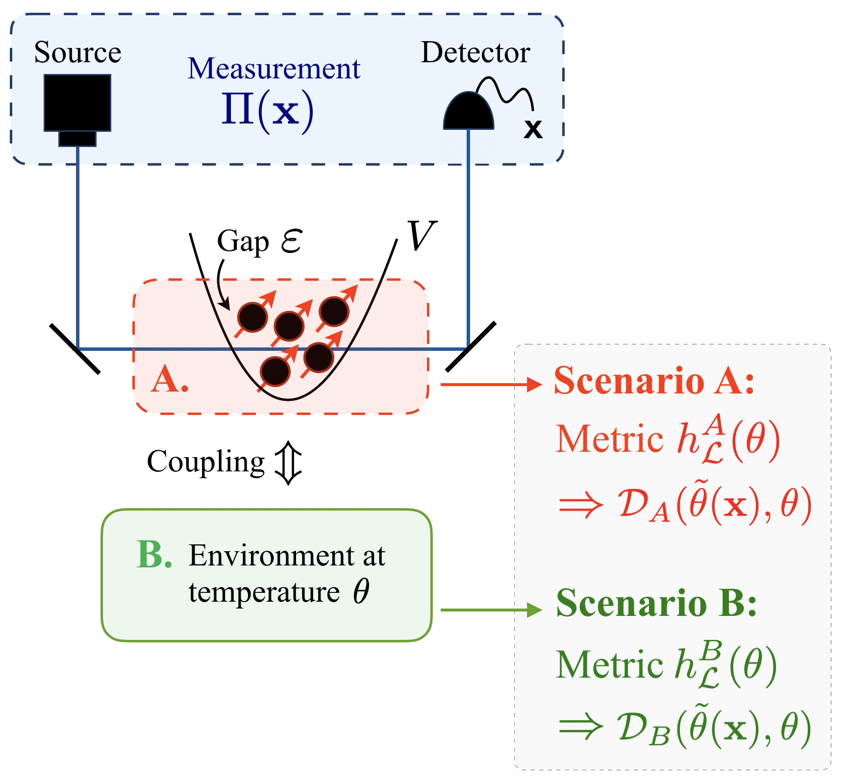
Figure 1: Illustration of a hypothetical experiment: A collection of spin impurities (A) interact with a thermal environment (B) at temperature $\theta$, the spin impurities are measured via an optical setup yielding measurement data x. An essential message of this paper is that the sample system defines the appropriate distance function, and that the distance is the basis of the estimation theory. To illustrate this point we consider two scenarios: (A) The spin impurities themselves constitute the sample-system of interest, e.g., we are interested in thermometry of the spin degrees of freedom themselves Hartke et al. (2020); Weld et al. (2009), in this case we obtain a metric $h_{\mathcal{L}}^{A}$ and a distance $\mathcal{D}_{A}$. (B) The spin impurities are employed as equilibrium thermometers of the thermal environment Bouton et al. (2020); Olf et al. (2015), in this case we obtain a different metric $h_{\mathcal{L}}^{B}$ and a different distance $\mathcal{D}_{B}$. As a consequence, the relevant figure of merit, and associated optimal protocol, will be different in each sensing process.

II Bayesian estimation theory

In this section we summarize the key concepts of Bayesian estimation theory Van Trees and Bell (2007); von Toussaint (2011). The aim of estimation theory, at least when considering point estimation Lehmann and Casella (1998), is to provide a prescription for singling out an estimate, serving as a best guess of an unknown quantity of interest, and for quantifying a measure of confidence in, or the precision of, the specified estimate. In this work, we specifically consider a smooth manifold of quantum states, e.g., thermal Gibbs states, of a sample—depicted schematically as $\mathcal{S}$ in Fig. 2. Our task is to estimate the true state of the sample, assuming that this belongs to the specified manifold.

Within the Bayesian theory, the manifold of states is equipped with a probability distribution, and this distribution is updated as measurement data is acquired. An estimate is computed, according to some prescription, based on the updated probability distribution. Providing a measure of confidence in an estimate, requires a notion of distance between states on the manifold. Here, we first argue for a metric structure on the manifold of states. A distance function can then be constructed as the geodesic length between states. As a result, the confidence in the computed estimate can then be unambiguously quantified via the mean-square distance over the updated probability distribution.

Having established the required notions of estimation theory, we provide a criterion for the optimal measurement design, and show how the local estimation theory can be recovered as the asymptotic limit of the Bayesian framework. Moreover, we outline a number of known results on Bayesian Cramér-Rao bounds that are particularly useful. Lastly, we discuss how to select an uninformative initial prior probability distribution.

II.1 Manifold of states and Bayesian updating

Physical systems are typically subject to a set of experimental conditions, e.g., some preparation procedure, which defines a smooth manifold of states Gallavotti (1999); Guarnieri et al. (2019); Brenes et al. (2020). To be specific we consider a quantum system, the sample, and assume that the true, but unknown, state of the sample $\rho_{\text{true}}$, belongs to a one-parameter family $\mathcal{S}_{\Theta}$ of quantum states in the manifold

$$\rho_{\text{true}}\in\mathcal{S}_{\Theta}\coloneqq\left\{\tau_{\Theta}(\theta)\ \ \text{for}\ \ \theta\in\Theta\right\},$$ (1)

where $\tau_{\Theta}(\theta)$ labels a parameterized quantum state, i.e., a linear operator on the sample Hilbert space, and $\Theta\subseteq\mathbb{R}$ denotes the parameter space, e.g., $\Theta$ could be the space of temperatures. Our task is to identify the true sample state, which, given that the state belongs to a one-parameter family, can be formulated as a parameter estimation problem. Throughout, we focus on a one-dimensional parameter space, and leave the generalization to the multi-dimensional case for future work.

Within Bayesian estimation theory we start from a prior probability density $p(\theta)$ on the parameter space $\Theta$, which is subsequently updated as the sample state is probed via measurements. Quantum mechanically, any measurement can be represented by a positive operator-valued measure (POVM). If we suppose that the sample is in the state $\tau_{\Theta}(\theta)$, then the likelihood $p(x\!\mid\!\theta)$ of observing a measurement outcome $x$ is given by Born’s rule

$$p(x\!\mid\!\theta)=\Tr\left[\Pi(x)\tau_{\Theta}(\theta)\right],$$ (2)

where $\Pi(x)$ is the POVM element associated with the outcome $x\in X$, and $X$ is the outcome space of the measurement performed. The POVM elements must be positive semi-definite, i.e. $\Pi(x)\geqslant 0$, and satisfy the normalization condition $\int_{X}dx\Pi(x)=\mathbb{I}$ with $\mathbb{I}$ being the identity operator Ballentine (2014). Conditioned on observing the specific outcome $x$, we can find the posterior probability distribution using Bayes’ rule:

$$p(\theta\!\mid\!x)=\frac{p(x\!\mid\!\theta)p(\theta)}{p(x)},$$ (3)

where $p(x):=\int_{\Theta}d\theta p(x\!\mid\!\theta)p(\theta)$ is the marginal probability density on the space of outcomes. For later use we also define the joint density $p(\theta,x)=p(x\!\mid\!\theta)p(\theta)$. The posterior density represents our degree of belief in different parameter values given the available measurement data. Note that here we formulate Bayes’ rule as a single-shot update. If we consider $\nu$ independent measurements giving outcomes $\textbf{x}=\left\{x_{1},...,x_{\nu}\right\}$, then it is equally valid to compute the posterior conditioned on the full set of observations.

II.2 Parameterization invariance

Having introduced the manifold of quantum states, and discussed probability densities on the parameter space, we must face the subtlety of parameterization invariance. In the above we work with a parameterization $\Theta$, however the manifold of quantum states itself is invariant with respect to the specific choice of parameterization. For example, the manifold of thermal Gibbs states is the same whether we parameterize it using the temperature or the inverse temperature. This fact is illustrated in Fig. 2. In general we can express this invariance as follows: if we consider a one-to-one mapping $\phi\!:\!\Theta\!\rightarrow\!\Phi$, where $\Phi\subseteq\mathbb{R}$ is the image of the map, then the function $\phi$ provides an equally valid parameterization of the manifold of states, i.e., $\mathcal{S}_{\Phi}\equiv\mathcal{S}_{\Theta}$ with

$$\mathcal{S}_{\Phi}=\left\{\tau_{\small{\Phi}}(\phi)\ \ \text{for}\ \ \phi\in\Phi\right\},$$ (4)

and we explicitly indicate that each state is now given with respect to the parameterization $\Phi$, while the invariance condition reads:

$$\forall\phi:\,\phi=\phi(\theta),\quad\tau_{\Theta}(\theta)=\tau_{\small{\Phi}}(\phi),$$ (5)

and expresses the parameterization invariance of every equivalent quantum state. Furthermore, the probability assigned to a given region of state space must be independent of the specific parameterization employed. Thus, to be consistent, the prior probability density must satisfy the invariance condition von Toussaint (2011); Jermyn (2005):

$$\forall\phi:\,\phi=\phi(\theta),\quad d\theta p_{\Theta}(\theta)=d\phi p_{\Phi}(\phi)$$ (6)

Since the likelihood function, $p(x|\theta)$, only depends on the state itself, it is inherently parameterization invariant. Hence, it thus follows that if the above invariance condition holds for the prior density it will also hold for the posterior density. To simplify our notation we will for the most part not indicate the parameterization explicitly in what follows. The choice of parameterization is implicitly indicated by the parameter value itself.

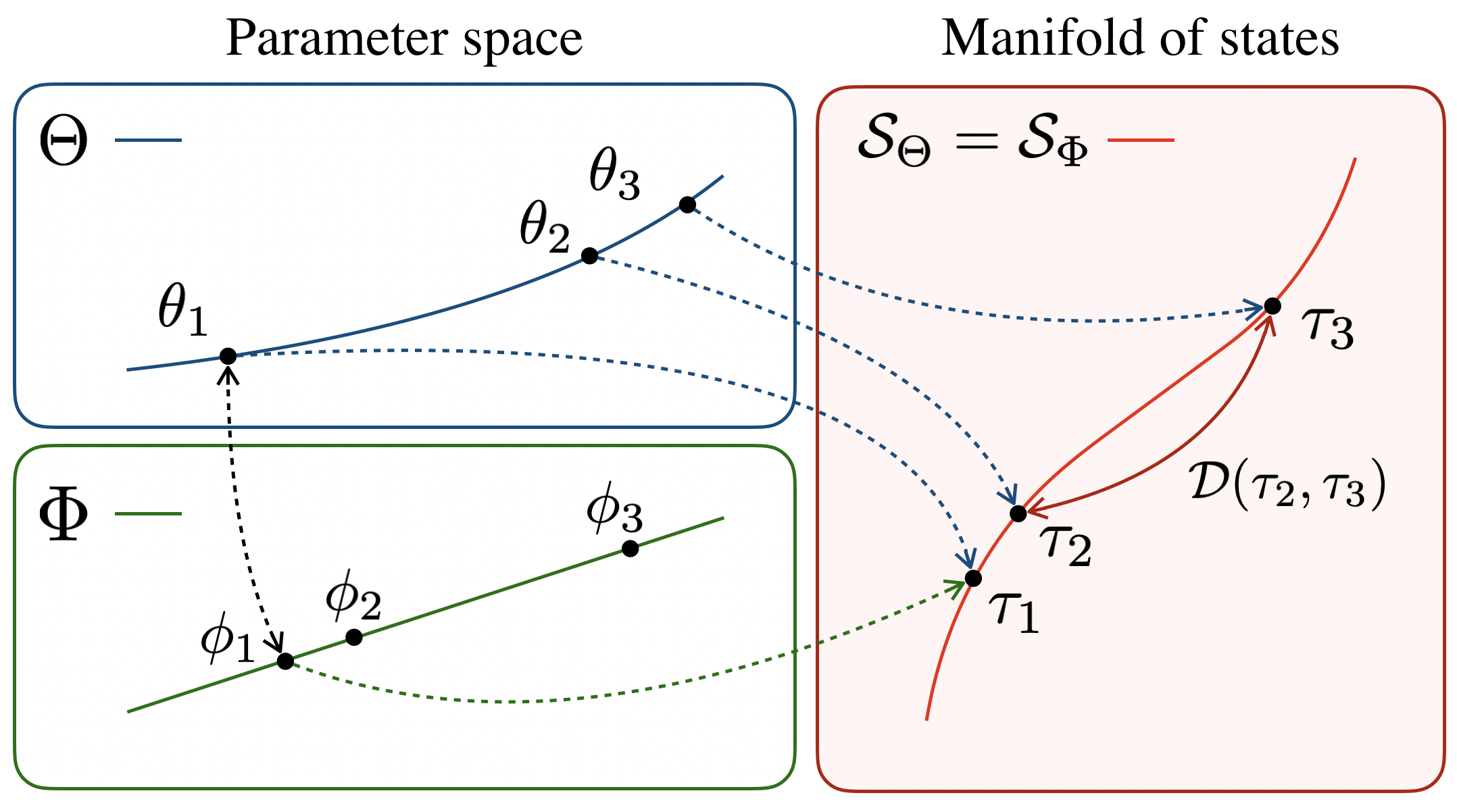
Figure 2: Illustration of a parameter space $\Theta$, or an alternative parameterization $\Phi$, mapped into a one-parameter curve of quantum states $\mathcal{S}_{\Theta}=\mathcal{S}_{\Phi}$. The distinguishability of parameter values is only meaningful, when expressed as a distance $\mathcal{D}$ between the corresponding quantum states, i.e., the state space induces a geometry on the parameter space. The induced geometry may be simpler for certain choices of parameterization. In particular, there may exist a Euclidean parameterization with a flat geometry. By considering the distance directly between quantum states, it follows that the distance is invariant with respect to the specific choice of parameterization of the states.

II.3 Metric structure and the geodesic length

The essential ingredient required for the development of a parameterization-invariant estimation theory on a Riemannian manifold is the metric structure, i.e., an infinitesimal notion of length, on the manifold of quantum states Jermyn (2005); Amari and Nagaoka (2007); Amari (1985). A metric makes it possible to define the distance between states on the manifold, and more fundamentally, the idea of defining a probability density on a continuous parameter space, is not well-defined in the absence of such a metric structure Jermyn (2005). Suppose for a moment that the manifold possesses a metric denoted by $g$. Then, it is always possible to construct a well-defined distance function, as the geodesic length – which we refer to as the metric-based distance – defined by Jermyn (2005); Amari (1985); Crooks (2007)

$$\mathcal{D}(\tau(\theta_{0}),\tau(\theta_{1}))\coloneqq\absolutevalue{\int_{\theta_{0}}^{\theta_{1}}d\theta\ g_{\Theta}(\theta)},$$ (7)

where the quantity $d\theta g_{\Theta}(\theta)$ provides a parameterization-invariant integration measure, i.e., $d\theta g_{\Theta}(\theta)=d\phi g_{\Phi}(\phi)$ for $\phi=\phi(\theta)$. The metric-based distance is a statistical distance between quantum states, and it is a parameterization-invariant quantity – this is depicted in Fig. 2. To simplify our notation, in what follows we will write the metric-based distance as $\mathcal{D}(\theta_{0},\theta_{1})$, referring only to the parameter values. However, it should be kept in mind that this is a distance between quantum states. The form of the geodesic length above is valid for one-parameter problems. More generally, defining the geodesic length involves a minimization over paths Jermyn (2005).

The above way of defining a distance function on the parameter space may still seem ambiguous unless a particular choice of metric can be justified. However, if we consider a reference measurement of the sample with POVM elements $\mathcal{M}(y)$ for $y\in Y$, then a key insight of Bayesian information geometry Snoussi (2007); Amari (1985); Jermyn (2005); Crooks (2007) is that the likelihood associated with this measurement, induces a metric of the form $g^{2}=h_{\mathcal{M}}$, where $h_{\mathcal{M}}$ is the Fisher information (FI) associated with the $\mathcal{M}$ measurement Jermyn (2005); Amari (1985); Paris (2009)

$$h_{\mathcal{M}}(\theta)=\int_{Y}dy\ p(y\!\mid\!\theta)\left(\partial_{\theta}\log p(y\!\mid\!\theta)\right)^{2}.$$ (8)

From the point of view of Bayesian probability theory, the Fisher information metric with respect to the reference measurement, is the unique Riemannian metric which satisfies both parameterization-invariance and any other invariance property of the likelihood function Jermyn (2005); Jarzyna and Kołodyński (2020). Moreover, according to Chentsov’s theorem, any other (monotonic) metric on the parameter space corresponds to the Fisher information metric, with respect to some reference measurement, up to a multiplicative constant Jarzyna and Kołodyński (2020); Chentsov (1978).

II.3.1 Quantum Fisher information metric

The choice of reference measurement represents a degree of freedom, i.e., we can define the metric-based distance, and the estimation theory itself, relative to an arbitrary reference measurement of the sample. A natural choice would be to maximize the distance $\mathcal{D}(\theta_{0},\theta_{1})$ over all possible measurements, however this procedure does not generally yield a unique reference measurement. To see this, we consider the problem of maximizing the metric at a specific parameter value. This local maximization problem can be solved analytically, and yields a metric defined relative to a projective measurement of the symmetric logarithmic derivative $\mathcal{L}(\theta)$ associated with the manifold of states Braunstein and Caves (1994). The symmetric logarithmic derivative (SLD) is defined implicitly by the relation Braunstein and Caves (1994):

$$\mathcal{L}(\theta)\tau(\theta)+\tau(\theta)\mathcal{L}(\theta)=2\partial_{\theta}\tau(\theta),$$ (9)

and is in general a function of the parameter value. The problem alluded to above is then that the SLD defines a natural reference measurement only if the eigenbasis of the SLD is parameter independent, i.e., the projectors must be parameter independent. Notice that this need not be the case for the SLD eigenvalues.

If we adopt the SLD reference measurement, then with this choice of reference we obtain the quantum Fisher information (QFI) metric, which gives the maximal likelihood-induced metric-based distance between sample states. The QFI metric is given by Braunstein and Caves (1994):

$$\sqrt{h_{\mathcal{L}}(\theta)}=\Tr[\mathcal{L}(\theta)^{2}\tau(\theta)]^{1/2}.$$ (10)

The resulting metric is equal to four times the Bures metric Paris (2009), and is thus directly related to the so-called fidelity between infinitesimally separated states in the manifold. If the family of states considered is a thermal state ensemble, then the metric-based distance is also called the thermodynamic length Weinhold (1975); Salamon and Berry (1983); Crooks (2007); Scandi and Perarnau-Llobet (2019). In the remainder of this paper we will always consider the SLD reference measurement, written $\mathcal{L}$, and the QFI metric following from that choice.

II.4 Choosing the correct Bayesian error

Having equipped the manifold with a metric structure, and outlined how to construct a metric-based distance function, we can develop a parameterization-invariant estimation theory by considering the mean-square distance as a suitable Bayesian error-function Jermyn (2005). Before proceeding with this development, we want to stress the basic logic of the approach. For a specific thermal sample system, the QFI metric associated with the SLD reference measurement specifies the thermodynamic geometry, i.e. it specifies how to measure the distance between thermal sample states. Only once the states are defined whose temperature should be distinguished (the manifold of states), is it possible to define the correct corresponding Bayesian error function.

II.4.1 Mean-square distance within the $\lambda_{\mathcal{L}}$ parameterization

In this section we consider an implemented measurement $\Pi$ giving measurement data $x$, and the SLD reference measurement $\mathcal{L}$ defining the thermodynamic length. Suppose we denote the estimator of the true parameter value constructed using the measurement data $x$ as $\tilde{\theta}(x)$. Then, we may define the mean-square distance based on Eq. (7) as

$$\text{\footnotesize{MSD}}(\tilde{\theta};x)\;\coloneqq\int_{\Theta}d\theta\ p(\theta\!\mid\!x)\ \mathcal{D}(\tilde{\theta}(x),\theta)^{2},$$ (11)

which provides a parameterization-invariant measure of the confidence assigned to the adopted parameter estimate. The mean-square distance is defined with respect to the likelihood function $p(x|\theta)$ associated with the implemented measurement $\Pi$, and it is defined with respect to the distance function associated with the SLD reference measurement $\mathcal{L}$. Furthermore, note that the mean-square distance is conditional on the measurement data, i.e., it is a stochastic quantity.

For convenience we define, implicitly, the function $\lambda_{\mathcal{L}}(\theta)$ as the inverse derivative of the QFI metric associated with the measurement $\mathcal{L}$ as Jermyn (2005)

$$\partial_{\theta}\lambda_{\mathcal{L}}(\theta)\coloneqq h^{1/2}_{\mathcal{L}}(\theta).$$ (12)

Since the QFI is non-negative it follows that the function $\lambda_{\mathcal{L}}$ is monotonically increasing. Furthermore, if we consider a change of parameterization $\theta\rightarrow\phi$, and note that under such a transformation the QFI transforms as $h_{\mathcal{L}}(\theta)=[\partial_{\theta}\phi]^{2}h_{\mathcal{L}}(\phi)$, then we see that it follows directly from the definition of $\lambda_{\mathcal{L}}$ that it is a parameterization-invariant quantity, i.e., $\lambda_{\mathcal{L},\Theta}(\theta)=\lambda_{\mathcal{L},\Phi}(\phi)$ for $\phi=\phi(\theta)$. Using the $\lambda_{\mathcal{L}}$ function it is always possible to express the distance (7) defined based on the QFI metric in the Euclidean form, i.e.:

$$\mathcal{D}(\tilde{\theta},\theta)=\absolutevalue{\lambda_{\mathcal{L}}(\tilde{\theta})-\lambda_{\mathcal{L}}(\theta)}.$$ (13)

This follows directly from an application of the fundamental theorem of calculus for $g_{\Theta}(\theta)=\sqrt{h_{\mathcal{L}}(\theta)}$.

If we constrain ourselves to reference measurements for which the QFI is non-vanishing (except perhaps at isolated points, e.g., the boundaries of the parameter domain), then $\lambda_{\mathcal{L}}$ itself constitutes a valid parameterization of the one-parameter family within the manifold. Referring to the associated parameter space as $\Lambda_{\mathcal{L}}$, it follows that when working in this parameterization the MSD takes the simple form:

$$\text{\footnotesize{MSD}}(\tilde{\lambda};x)\;=\int_{\Lambda_{\mathcal{L}}}d\lambda\ p(\lambda\!\mid\!x)\ (\tilde{\lambda}(x)-\lambda)^{2},$$ (14)

where $\tilde{\lambda}(x)=\lambda(\tilde{\theta}(x))$, and we have made use of Eq. (6), i.e., the invariance property of the posterior probability density function. In the above we dropped the subscript $\mathcal{L}$ when referring to the $\lambda$ parameter itself. Furthermore, from here on we will not explicitly indicate the space which is integrated over, i.e. $\Lambda_{\mathcal{L}}$. Note that the $\Lambda_{\mathcal{L}}$-parameterization is special in that it is associated with a QFI equal to unity, i.e., a flat metric. The form of the MSD is then simply the standard Euclidean distance with respect to the parameterization $\Lambda_{\mathcal{L}}$.

The remaining open question is how to choose a suitable estimation function. A natural choice, and the one primarily adopted here, is the mean of $\lambda$ over the posterior probability distribution

$$\bar{\lambda}(x)\;\ \coloneqq\int d\lambda\ p(\lambda\!\mid\!x)\ \lambda.$$ (15)

It can be shown that this choice of estimation function is classically optimal, in the sense that it minimizes the mean-square distance (Eq. (14)) Van Trees and Bell (2007); Jermyn (2005); Kay (1993). For this reason the posterior mean of $\lambda$ is called the minimal mean-square distance (MMSD) estimator Jermyn (2005). Notice that since the MSD is a parameterization-invariant quantity, we can then directly obtain the corresponding MMSD estimate of $\theta$ as $\bar{\theta}(x)=\lambda^{-1}\bar{\lambda}(x)$, where $\lambda^{-1}$ denotes the inverse of the function $\lambda$.

II.4.2 The expected mean-square distance

Having introduced the mean-square distance as a measure of confidence, the next problem is to identify a suitable criterion for optimal measurement design. We immediately face the difficulty that the mean-square distance is a stochastic quantity, i.e., in identifying the optimal measurement one must consider the full ensemble

$$\Xi\equiv\left\{\text{\footnotesize{MSD}}(\bar{\lambda};x)\ \ \text{for}\ \ x\in X\right\}.$$ (16)

In an actual experiment we sample this ensemble according to the likelihood $p(x\!\mid\!\theta_{\text{true}})$ with respect to the true quantum state of the sample. Since the true state is unknown a priori, we cannot gauge the expected confidence in an estimate resulting from a measurement based on the true likelihood. Instead we must assume that the ensemble $\Xi$ is sampled according to the marginal density $p(x)$, giving the likelihood averaged over the prior density.

In the simplest case we suppose that the ensemble $\Xi$ is well captured by its average behaviour, which constitutes a deterministic quantity, typically referred to as the Bayesian mean-squared error Kay (1993); Van Trees and Bell (2007). As in our work we interpret it as the average evaluated over the marginal density of the MSD (14), we refer to it as the expected mean-square distance (EMSD), i.e.:

$$\text{\footnotesize{EMSD}}[\bar{\lambda}] \coloneqq\int\!dx\;p(x)\;\text{\footnotesize{MSD}}(\tilde{\lambda};x)$$ (17)

$$=\int\!d\lambda\,dx\ p(\lambda,x)\ \left(\bar{\lambda}(x)-\lambda\right)^{2},$$ (18)

where we use square brackets to denote the choice of estimator. Hence, a natural criterion for determining the optimal measurement design is to minimise the EMSD. Note that the optimal measurement will generally be a functional of the prior probability distribution, or in other words the optimal choice of measurement depends on the prior knowledge.

II.5 Connection to the local paradigm

We now consider the local limit of a narrow posterior distribution. In this limit the EMSD is lower bounded, and typically well approximated, by the expected Cramér-Rao bound (ECRB) Bacharach et al. (2019); Braunstein and Caves (1994). To derive this bound, we first rewrite the EMSD as

$$\text{\footnotesize{EMSD}}[\tilde{\lambda}]=\int d\lambda p(\lambda)\Delta^{2}\tilde{\lambda},$$ (19)

where we have decomposed the joint probability and defined the “frequentist” mean-square error (MSE) Kay (1993)

$$\Delta^{2}\tilde{\lambda}\coloneqq\int dx\ p(x|\lambda)[\tilde{\lambda}(x)-\lambda]^{2}.$$ (20)

Adopting an asymptotically unbiased estimator, implies that the MSE satisfies the Cramér-Rao bound Kay (1993), and upon substitution we obtain the ECRB:

$$\text{\footnotesize{EMSD}}[\tilde{\lambda}_{\text{ub}}]\geqslant\footnotesize{\text{ECRB}} \coloneqq\int d\lambda\frac{p(\lambda)}{h_{\Pi}(\lambda)}$$ (21)

$$\ =\int d\theta\ p(\theta)\frac{h_{\mathcal{L}}(\theta)}{h_{\Pi}(\theta)},$$

where $\tilde{\lambda}_{\text{ub}}$ denotes any unbiased estimator, and we recall that $h_{\Pi}$ is the Fisher information associated with the implemented measurement. The final equality follows from a change of parameterization, and an application of Eq. (12). The ECRB is typically tight in the asymptotic limit, i.e., the limit of a large number of measurement repetitions Bacharach et al. (2019).

The expression for the ECRB given here offers a generalization of the results reported in Mok et al. (2020); Rubio et al. (2020) — these corresponds to $h_{\mathcal{L}}(\theta)\propto 1$ and $h_{\mathcal{L}}(\theta)\propto\theta^{-2}$ respectively. The ECRB shows that the EMSD converges to a generalized version of the relative error averaged over the prior probability, i.e., relative to the metric structure of the manifold. Note that the ECRB shows that the noise-to-signal ratio is only meaningful if the geometry of the problem is scale invariant, i.e. $h_{\mathcal{L}}(\theta)\propto\theta^{-2}$. For general geometries a physically meaningful notion of relative error is given by the mean-square distance. This insight alters the data analysis even in the asymptotic limit.

II.6 Bayesian Cramér-Rao bounds

As noted above, the expected thermometric performance is naturally quantified via the EMSD, and the optimal measurement strategy is the one for which the EMSD is minimal. As an alternative to directly considering the EMSD, we can assess the expected performance by studying bounds on the attainable precision. In many cases this is computationally advantageous. The cost of considering lower bounds is that we do not know in general if the EMSD saturates them.

An advantage of working in the $\Lambda_{\mathcal{M}}$-parameterization is that the EMSD takes the form, as mentioned, of the BMSE. The EMSD can then be directly lower bounded by means of the so-called Van-Trees inequalities Van Trees and Bell (2007), which are valid when $p(\lambda)$ and $\lambda p(\lambda)$ vanish at the boundaries of $\Lambda_{\mathcal{M}}$. We first consider the tightened Bayesian Cramér-Rao bound (TBCRB) Bacharach et al. (2019); Li et al. (2018)

$$\text{\footnotesize{EMSD}}[\bar{\lambda}]\geqslant\text{\footnotesize{TBCRB}}\coloneqq\int dx\ p(x)\mathcal{Q}(x)^{-1},$$ (22)

given in terms of the Bayesian information

$$\mathcal{Q}(x)=\int d\lambda\ p(\lambda\!\mid\!x)\left[\partial_{\lambda}\log p(\lambda\!\mid\!x)\right]^{2}.$$ (23)

The EMSD saturates the TBCRB, i.e., the bound is tight, when the posterior probability density takes the form of a Gaussian distribution in the $\Lambda_{\mathcal{M}}$-parameterization with inverse variance $\mathcal{Q}(x)$ Bacharach et al. (2019). According to the Laplace-Bernstein-von Mises theorem, this condition is satisfied in the asymptotic limit Li et al. (2018).

Evaluating the TBCRB is in general no less demanding than computing the EMSD, and our reason for starting with the TBCRB is that it comes with a condition for when it is tight. Often it is more convenient to consider the Bayesian Cramér-Rao bound (BCRB), which is obtained via an application of Jensen’s inequality Bacharach et al. (2019, 2019)

$$\text{\footnotesize{TBCRB}}^{-1} \leqslant\text{\footnotesize{BCRB}}^{-1}$$ (24)

$$\coloneqq Q_{\text{prior}}+\int d\theta\ p(\theta)\frac{h_{\Pi}(\theta)}{h_{\mathcal{M}}(\theta)},$$

where the prior information content is quantified by

$$Q_{\text{prior}}=\int d\lambda\ p(\lambda)\ \left[\partial_{\lambda}\log p(\lambda)\right]^{2},$$ (25)

which is simply the Bayesian information evaluated for the initial prior. The TBCRB saturates the BCRB if the Bayesian information function is a constant independent of the measurement data. The advantage of working in the $\Lambda_{\mathcal{M}}$-parameterization is that the derived bound is automatically parameterization invariant.

Both the TBCRB and the BCRB are applicable at the single-shot level of the measurement protocol. In many cases the TBCRB is as difficult to compute as the EMSD, this leaves BCRB-optimization as a viable choice of optimization strategy.

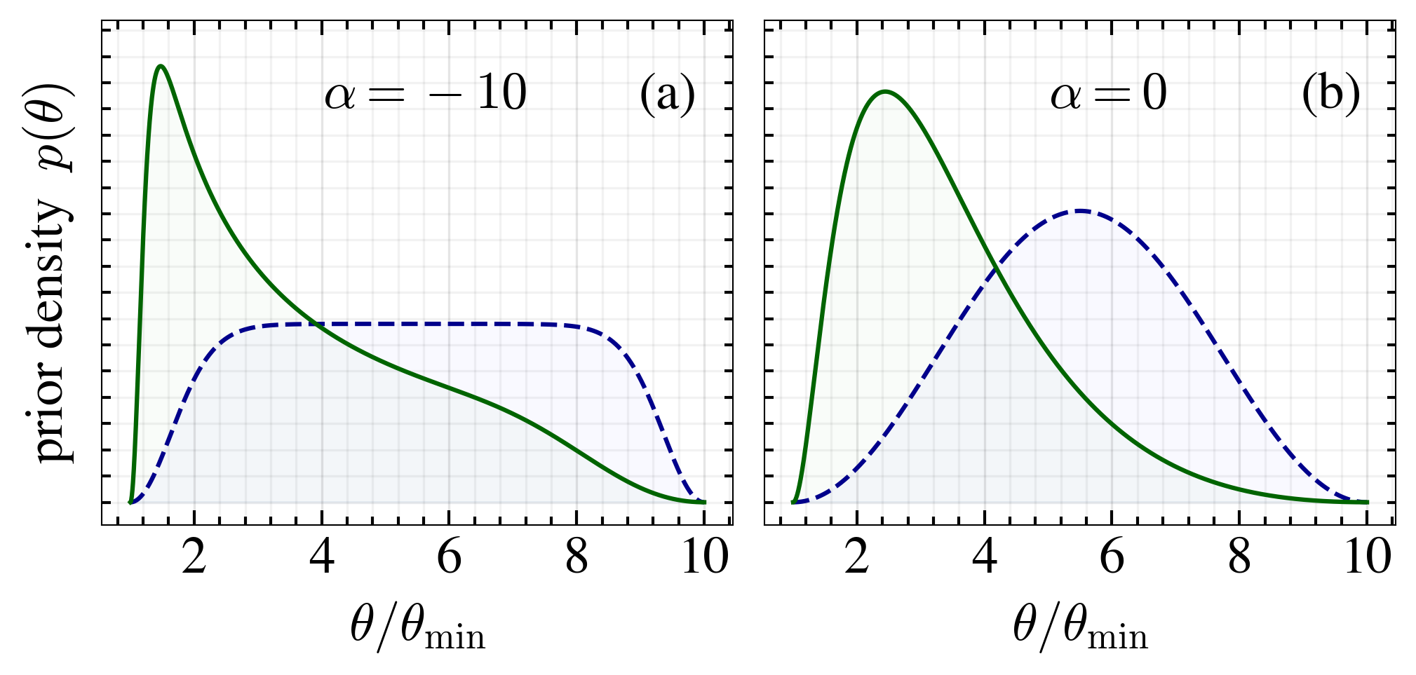
Figure 3: Illustration of the smoothed Jeffrey’s prior (Eqs. (26) and (27)) for a flat reference $h_{\mathcal{L}}(\theta)\propto 1$ (dashed blue lines) and a curved metric $h_{\mathcal{L}}(\theta)\propto 1/\theta^{2}$ (solid green lines) (a) Plot for $\alpha=-10$, in this limit we approach an equal a priori probability postulate on the bounded interval $\theta\in[\theta_{\min},\theta_{\max}]$. For a flat metric this gives a constant prior density with smoothed boundaries. For the curved metric the prior density is concentrated at small parameter values as the metric assigns the majority of metric length to this regime. (b) Plot for $\alpha=0$. In this regime, the prior resembles a Gaussian distribution on a bounded interval.

II.7 Specifying the initial prior

Within the Bayesian approach, prior densities are updated to posterior densities as measurement data is acquired. Applying the Bayesian framework requires specifying an initial prior, and it is crucial to choose a prior which correctly represents ones prior knowledge, or does not strongly effect the inference process. If we recall that the QFI metric encodes the thermodynamic geometry of the sample space, then it is convenient to express a general prior as a product

$$p(\theta)=h_{\mathcal{L}}^{1/2}(\theta)f(\theta),$$ (26)

where $f(\theta)$ is a parameterization-invariant density. If we are interested in applying an equal a priori probability postulate on a specific domain of parameter space, i.e., we want an uninformative prior over the specified domain, then this corresponds to having a constant, $f(\theta)=\text{cons.}$, prior density on this domain. For a constant density the prior is proportional to the QFI metric, or in other words, the probability assigned to an infinitesimal parameter interval is proportional to the length of the interval. In this case we recover the so-called Jeffrey’s prior, which is the prior expressing complete ignorance given the metric structure of the parameter space Caticha (2008). For all simulations performed in the next section we adopt a smoothed density

$$f(\theta)=\frac{1}{\mathcal{N}}\left(\exp\left[\alpha\sin^{2}\left(\pi\frac{\lambda(\theta)-\lambda_{\min}}{\lambda_{\max}-\lambda_{\min}}\right)\right]-1\right)$$ (27)

with a normalization factor given by

$$\mathcal{N}\equiv(\lambda_{\max}-\lambda_{\min})\left[\exp(\alpha/2)I_{0}(\alpha/2)-1\right]$$ (28)

where $\theta\in[\theta_{\min},\theta_{\max}]$, $\lambda_{\text{min,max}}=\lambda(\theta_{\text{min,max}})$ respectively and $I_{0}$ is the modified Bessel function of the first kind. The resulting prior is essentially the one studied by Yan et al. Li et al. (2018), however we specify the density with respect to the Euclidean parameterization. In the limit of large negative $\alpha$, the density goes to a constant on the parameter domain, and we thus recover Jeffrey’s prior. The prior is illustrated in figure 3 for a flat reference metric $h_{\mathcal{L}}(\theta)\propto 1$ and a curved reference metric given by $h_{\mathcal{L}}(\theta)\propto\theta^{-2}$.

III Applications

In this section, we consider some applications of the above estimation theory to the problem of thermometry. First, we argue for a suitable form of the reference metric when the sample system can be represented as a thermalizing channel, and show that in this case the relative error is given by the standard noise-to-signal ratio. Second, we consider the case of thermal spin-$1/2$ particles, and illustrate the difference between a thermometric scenario in which the spin-$1/2$ particles are considered as a thermometer for an underlying heat reservoir, and a scenario in which the spin-$1/2$ particles themselves constitute the sample-system of interest. These two scenarios correspond to scenario B and scenario A illustrated in Fig. 1.

III.1 Preliminaries

We consider the case where the one-parameter family of sample-system states is the thermal Gibbs states with respect to a Hamiltonian operator $H$, and take $\theta$ to denote the temperature. Recall that the Gibbs state takes the form Mehboudi et al. (2019b); De Pasquale and Stace (2018)

$$\rho(\theta)=\frac{\exp\left(-H/k_{B}\theta\right)}{\Tr\left[\exp\left(-H/k_{B}\theta\right)\right]}.$$ (29)

As our reference measurement we take a projective measurement of the SLD operator, which for Gibbs states takes the form Mehboudi et al. (2019b); De Pasquale and Stace (2018); Correa et al. (2015)

$$\mathcal{L}(\theta)=\frac{H-\Tr[\tau(\theta)H]}{2k_{B}\theta^{2}},$$ (30)

where $k_{B}$ is the Boltzmann constant. Measuring the SLD thus corresponds to a projective measurement of the sample-system energy. Noting that the Hamiltonian operator is temperature independent, and that this feature carries over to the eigenbasis of the SLD, it follows that a projective measurement of the SLD operator provides a valid reference measurement. For a projective energy measurement the associated FI, or equivalently the QFI, is then directly related to the sample-system heat capacity Mehboudi et al. (2019b); De Pasquale and Stace (2018); Correa et al. (2015), i.e.:

$$h_{\mathcal{L}}(\theta)=\frac{\partial_{\theta}\Tr[\tau(\theta)H]}{k_{B}\theta^{2}}\eqqcolon\frac{C(\theta;H)}{k_{B}\theta^{2}}.$$ (31)

The square-root of the QFI then provides a metric on the manifold of thermal Gibbs states. Recall that the associated metric-based distance is called the thermodynamic length Weinhold (1975); Salamon and Berry (1983); Crooks (2007); Scandi and Perarnau-Llobet (2019). Below we evaluate the thermodynamic length in the case of a bosonic mode and a spin-$1/2$ particle. First, however, we discuss how to represent a thermalizing channel.

III.2 The thermalizing channel

A common scenario in quantum thermometry, is that of a quantum probe subject to a thermalizing channel. A thermalizing channel can in general be modelled as induced by a sample-system which is effectively an infinitely large heat reservoir. Here we model such an ideal heat reservoir by a heat capacity which, either approximately or by definition, equals a constant value $k_{B}\mathcal{V}$ across the range of relevant temperatures, i.e., the sample energy is a linear function of the temperature. Note that a constant heat capacity corresponds to the QFI metric $h_{\mathcal{L}}(\theta)=k_{B}\mathcal{V}/\theta^{2}$. In this case we can evaluate the thermodynamic length analytically and find

$$\mathcal{D}(\theta_{0},\theta_{1})=\ \absolutevalue{\log(\theta_{1}/\theta_{0})},$$ (32)

where for convenience we set $\mathcal{V}=1$. The form of the MSD resulting from this distance function is called the mean-square logarithmic error $(\text{\small{MSLE}})$. The MSLE can be adopted whenever it can be assumed that the manifold of thermal states is generated via a weak coupling to an infinite heat reservoir. In practice this assumption might break down at low temperatures, and more fundamentally there are cases where thermal behaviour cannot be linked to an infinite heat reservoir, e.g., the case of subsystem thermalization described by the eigenstate thermalization hypothesis Brenes et al. (2020); Ashida et al. (2018).

The MSLE was recently proposed by Rubio et al. Rubio et al. (2020) as a suitable measure of confidence, in the special case of a reference measurement for which the associated likelihood function satisfies the scale-invariance property

$$p(x\!\mid\!\theta)=\frac{g(x/\theta)}{\int dx\ g(x/\theta)},$$ (33)

where $x$ denotes the outcome from a projective measurement of the sample energy and $g(x/\theta)$ is a function only of the dimensionless ratio $x/\theta$. This scale-invariance property of the likelihood function is satisfied for sample-systems with a constant density of states, or equivalently, a constant heat capacity.

When considering the MSLE, it follows that the reference QFI takes the form $h_{\mathcal{L}}(\theta)=\theta^{-2}$, and we then find that the associated ECRB for an unbiased estimator is given by

$$\text{\footnotesize{ECRB}}=\int d\theta\ \frac{p(\theta)}{\theta^{2}h_{\Pi}(\theta)}.$$ (34)

The quantity $\theta^{2}h_{\Pi}(\theta)$ provides an upper bound on the signal-to-noise ratio within the frequentist estimation paradigm Potts et al. (2019); Jørgensen et al. (2020). This shows that when the sample can be modelled as an ideal heat reservoir, the standard notion of relative error is recovered in the local limit where $p(\theta)$ is sharply peaked. However, our analysis also points out that the standard relative error is not suitable unless the sample-system has an approximately constant heat capacity across the range of relevant temperature. This condition typically breaks down at sufficiently low temperatures.

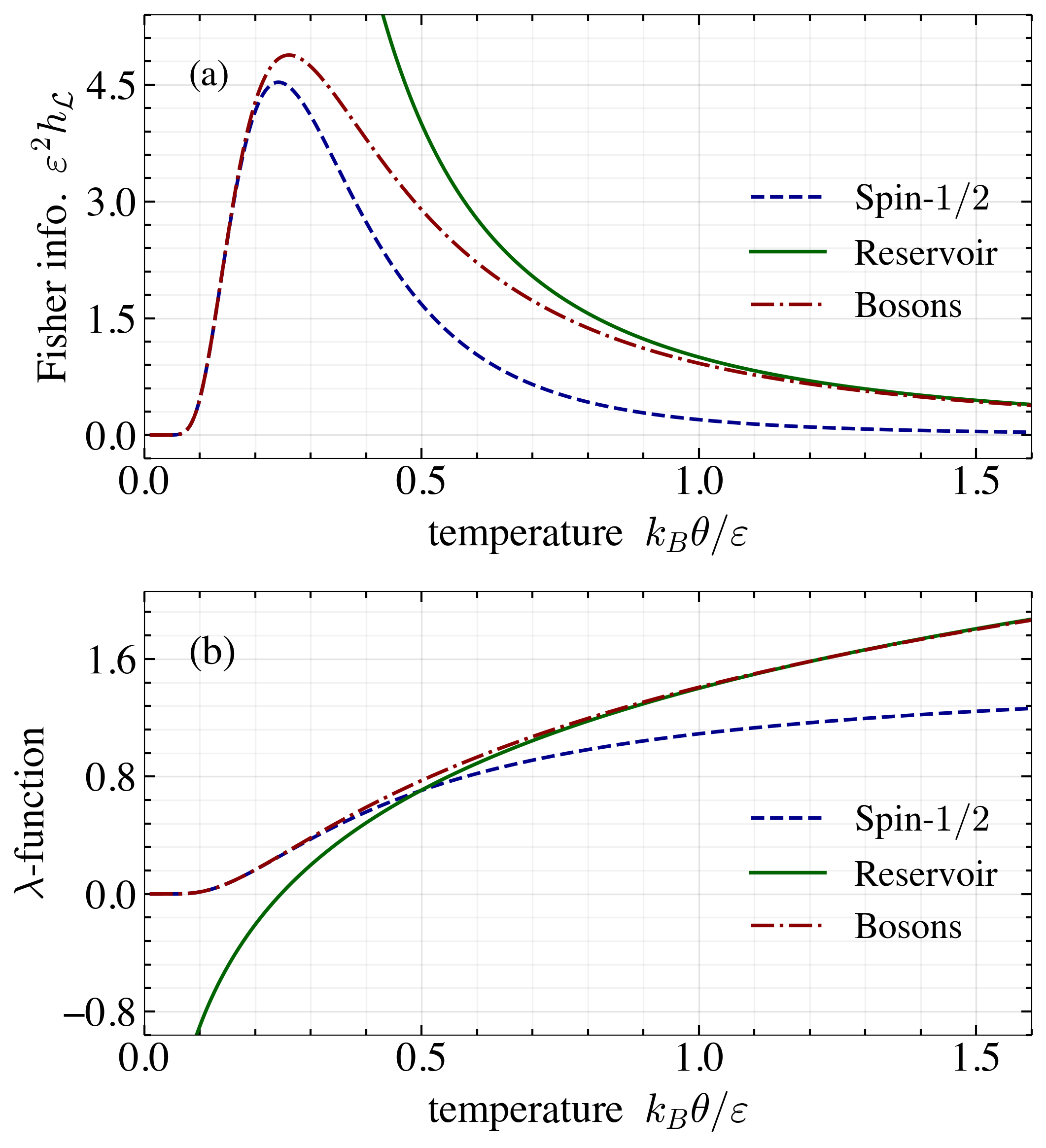
Figure 4: (a) Plot of the QFI for a spin-$1/2$ particle (dashed blue line), the QFI for a bosonic mode (dashed-dotted red line), and the QFI for the ideal heat reservoir (solid green line). (b) Plot of the $\lambda$-functions associated with the various QFIs.

III.2.1 Thermodynamic length for a Bosonic mode

A specific system approximately realizing the above assumptions on an ideal heat reservoir is a Bose gas at a fixed density well above the critical temperature Potts et al. (2019). As an illustration we consider a gas of bosonic modes with energy gap $\varepsilon$. In this case the QFI per mode is given by Mehboudi et al. (2019b)

$$h_{\mathcal{L},\text{boson}}(\theta)=\frac{\varepsilon^{2}/k_{B}^{2}\theta^{4}}{4\sinh^{2}(\varepsilon/2k_{B}\theta)}.$$ (35)

For this QFI the associated $\lambda$-function (see Eq. (12)) can be given an analytic expression

$$\lambda_{\text{boson}}(\theta)=-\log\left[\tanh\left(\varepsilon/4k_{B}\theta\right)\right],$$ (36)

which implies that $\Lambda_{\mathcal{L},\text{boson}}=[0,+\infty)$. The bosonic QFI and the associated $\lambda$-function are shown in figure 4(a) and figure 4(b), together with the corresponding quantities for an ideal heat reservoir. We observe that in the limit where the temperature is large compared to the boson energy gap, the bosonic modes approximate the ideal heat reservoir, i.e. $h_{\mathcal{L},\text{boson}}(\theta)\rightarrow 1/\theta^{2}$. This suggests that we can generically represent an ideal thermalizing channel physically by a collection of low-frequency bosonic modes.

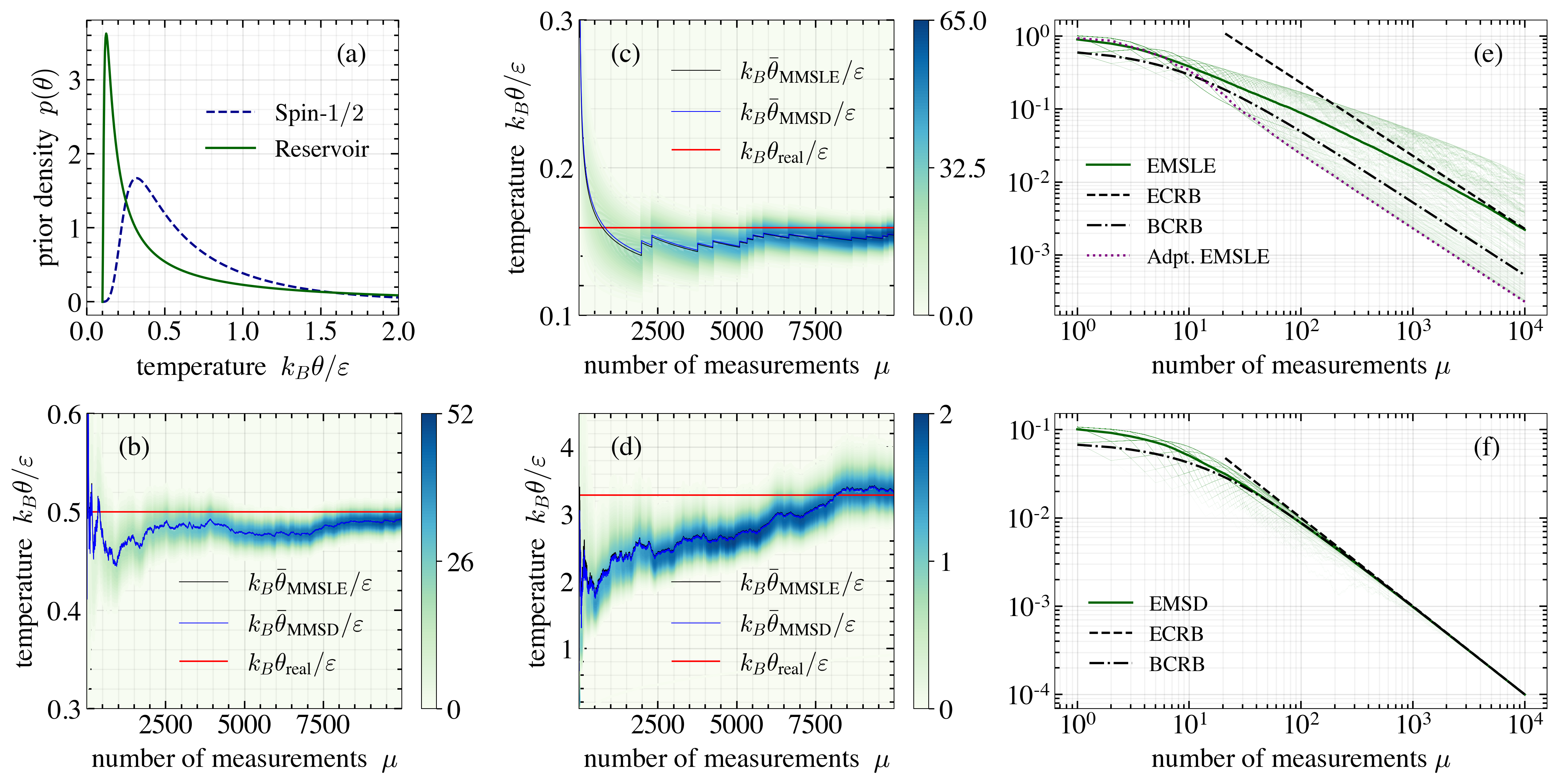
Figure 5: (a) The smoothed Jeffrey’s prior (Eqs. (26) and (27)) for $\alpha=-4.5$ and $k_{B}\theta\in[\varepsilon/10,10\varepsilon]$, corresponding to the spin-$1/2$ particle and the reservoir reference metric. (b,c,d) Simulated stochastic measurement trajectories sampled according to a specific true temperature (red horizontal line), the posterior probability density function is shown as a colour map. Both the MMSLE and the MMSD estimators are shown. (e) Simulation of the EMSLE (Scennario B) for thermometry employing free spin-$1/2$ particles. The simulation is performed by averaging over $250$ stochastic trajectories where the measurement data is generated with respect to a true temperature sampled according to the prior density. The EMSLE is compared with the ECRB, convergence is observed for $\mu\gtrsim 10^{3}$, and we note that the generated trajectories do not converge to the mean asymptotically. Furthermore, we plot the BCRB and observe that this is not a tight bound. Lastly, we plot the adaptive EMSLE. This is obtained by adapting the energy gap $\varepsilon$ in each repetition of the measurement. Here, we employ a BCRB optimization strategy which is described in more detail in the main text. (f) Simulation of the EMSD (Scenario A) for thermometry of free spin-$1/2$ particles. The simulation is performed by averaging over $250$ stochastic trajectories where the measurement data is generated with respect to a true temperature sampled according to the prior density. The EMSD is compared with the BCRB and convergence is observed for $\mu\gtrsim 10^{2}$, furthermore we observe that the generated trajectories converge to the average.

III.3 Non-interacting spin-$1/2$ particles

We now consider $N$ non-interacting spin-$1/2$ particles, or qubits, with identical energy gaps $\varepsilon$. The spin-$1/2$ particles are in a thermal Gibbs state, and as above we take the $\theta$ parameterization to be the temperature. We are going to compare and contrast two scenarios: (A) the spin-$1/2$ particles themselves constitute the sample-system of interest, e.g., we are interested in thermometry of the spin degrees of freedom of the ultracold atoms themselves Hartke et al. (2020); Weld et al. (2009), and (B) the spin-$1/2$ particles are employed as equilibrium thermometers of an underlying heat reservoir, e.g., the particles could model impurities within an ultracold gas, mapping motional information of gas atoms onto the quantum-spin state Bouton et al. (2020); Olf et al. (2015).

In case (B), as argued above, the MSLE is the suitable measure of confidence, and the QFI metric takes the form $h_{\mathcal{L},\text{res.}}(\theta)=\theta^{-2}$. In case (A) we take the MSD resulting from adopting the QFI metric of a thermal spin-$1/2$ particle as our reference, i.e., Potts et al. (2019)

$$h_{\mathcal{L},\text{spin}}(\theta)=\frac{\varepsilon^{2}/k_{B}^{2}\theta^{4}}{4\cosh^{2}(\varepsilon/2k_{B}\theta)},$$ (37)

which, we recall, corresponds to a projective energy measurement of a single spin-$1/2$ particle. When referring to the MSD below, we refer to the spin-$1/2$ particle QFI metric. For the spin-$1/2$ reference, the inverse derivative function $\lambda(\theta)$ can be obtained analytically, it takes the form

$$\lambda_{\text{spin}}(\theta)=\pi-2\arctan\left(e^{\varepsilon/2k_{B}\theta}\right),$$ (38)

and thus $\Lambda_{\mathcal{L},\text{spin}}=[0,\pi/2]$. In figure 4(a) we plot the spin-$1/2$ QFI and compare it with the heat reservoir reference, and in figure 4(b) we plot the associated $\lambda$-functions. We observe that for temperature around $k_{B}\theta/\varepsilon\approx 0.3$ the two $\lambda$-functions exhibit a similar gradient, however away from this temperature regime the specific thermometric scenario considered plays a role.

The estimation strategy employed consists of projectively measuring the energy of a subset of $\mu$ particles – this is written as number of measurements in Fig. 5. For thermalized spin-$1/2$ particles, projective energy measurements maximize the associated FI for all temperatures Paris (2015), and it follows that the FI associated with this measurement can be expressed as

$$h_{\Pi}(\theta)=\mu h_{\mathcal{L},\text{spin}}(\theta).$$ (39)

In figure 5(a), figure 5(b) and figure 5(c) we show stochastic simulations of measurement trajectories sampled according to three different true temperatures. In all cases we plot the MMSLE estimator and the MMSD estimator, and note that only negligible differences exist between these, despite different priors being used. This feature is to be expected as the respective $\lambda$-functions rapidly become approximately constant across the posterior, when this is the case the estimator is simply the maximum-a-posterior temperature, i.e., the temperature at which the posterior takes its maximum value, independently of the specific $\lambda$-function.

Although the various temperature estimates are only negligibly different, the confidence assigned to the estimates depend on the thermometric scenario. In figure 5(e) and 5(f) we show the EMSLE and the EMSD respectively as a function of the subset size $\mu$, or equivalently the number of independent measurements, and compare these with the associated BCRB and the associated ECRB. The EMSLE and the EMSD are evaluated using the corresponding smoothed Jeffrey’s priors shown in figure 5(d). In the case of the EMSLE we do not observe convergence to the BCRB. This is to be expected since $h_{\mathcal{L},\text{res.}}/h_{\Pi}$ is generally not constant across the domain of the employed prior. This feature also means that we do not observe a convergence to be ECRB at the trajectory level, i.e., we observe fluctuations around the average. For the EMSD we observe rapid convergence to the BCRB, and trajectory level convergence to the ECRB. This is due to the fact that $h_{\mathcal{L},\text{spin}}/h_{\Pi}=1/\mu$ is a constant independent of the temperature.

When considering the spin-$1/2$ particles as thermometers of a underlying heat reservoir, it is sensible to consider adaptation of the energy gap $\varepsilon$ to optimize the thermometric performance. That is we consider a protocol consisting of thermalizing a spin-$1/2$ particle and projectively measuring the energy. Based on the observed outcome, the energy gap of the particle employed in the following measurement is adapted. In figure 5(e) we also show the adaptive EMSLE, which is obtained via a BCRB optimization strategy of the spin-$1/2$ energy gap $\varepsilon$ in each iteration of the protocol. By a BCRB optimization strategy we refer to a minimization of the BCRB with respect to the energy gap $\varepsilon$ in each iteration. In this case we observe a rapid convergence to the optimized local result, i.e., the adaptive $\text{\footnotesize{EMSLE}}\sim\max_{\theta}[h_{\mathcal{L},\text{res.}}/h_{\Pi}]$. Furthermore, the adaptive EMSLE converges to a lower bound on the set of MSLE trajectories. This is to be expected as the energy gap can be tuned to the optimal ratio of the energy gap to the temperature sampled from the prior.

IV Conclusion

In this paper, we have developed a general Bayesian approach to quantum thermometry based on the concept of thermodynamic length. The basic idea is that a meaningful measure of the precision of a temperature estimate should be based on the ability to distinguish states at different temperatures, i.e., colder from hotter, and should be independent of the particular parameterization of the states, e.g., temperature. The theory allows us to meaningfully quantify the thermometric performance of a given measurement strategy, and to design optimal measurements under conditions of prior temperature uncertainty. Furthermore, the framework is applicable at the single-shot level, which allows us to consider adaptive measurement schemes. Insisting on a framework which satisfies both parameterization invariance and any other symmetry of the sample system considered leads us to gauge the thermometric performance using a distance function defined relative to the quantum Fisher information metric on the manifold of thermal states of the sample, i.e., the thermodynamic length. Formulating the problem in terms of the thermodynamic length, then leads to the realization that any meaningful notion of relative error must be given with respect to the specific sample system considered. Furthermore, we demonstrate that the suitability of both Bayesian and local Cramér-Rao bounds is contingent on the specific sample-system which is measured.

The generalization of the notion of relative error is particularly important in the low-temperature regime, where it shows that the standard signal-to-noise ratio is not a good indicator of estimation precision, and provides an alternative point of view on the problems of low-temperature quantum thermometry Jørgensen et al. (2020); Potts et al. (2019). In addition the generalization is important at the microscale, where we are often not interested in thermometry of ideal heat baths, but rather in characterizing the thermodynamics of operating quantum devices such as quantum simulators.

References

- Kucsko et al. (2013) G. Kucsko, P. C. Maurer, N. Y. Yao, M. Kubo, H. J. Noh, P. K. Lo, H. Park, and M. D. Lukin, “Nanometre-scale thermometry in a living cell,” Nature 500, 54–58 (2013).
- Fujiwara et al. (2020) Masazumi Fujiwara, Simo Sun, Alexander Dohms, Yushi Nishimura, Ken Suto, Yuka Takezawa, Keisuke Oshimi, Li Zhao, Nikola Sadzak, Yumi Umehara, Yoshio Teki, Naoki Komatsu, Oliver Benson, Yutaka Shikano, and Eriko Kage-Nakadai, “Real-time nanodiamond thermometry probing in vivo thermogenic responses,” Science Advances 6 (2020), 10.1126/sciadv.aba9636.
- Moreva et al. (2020) E. Moreva, E. Bernardi, P. Traina, A. Sosso, S. Ditalia Tchernij, J. Forneris, F. Picollo, G. Brida, Ž. Pastuović, I. P. Degiovanni, P. Olivero, and M. Genovese, “Practical applications of quantum sensing: A simple method to enhance the sensitivity of nitrogen-vacancy-based temperature sensors,” Phys. Rev. Applied 13, 054057 (2020).
- Carcy et al. (2021) Cécile Carcy, Gaétan Hercé, Antoine Tenart, Tommaso Roscilde, and David Clément, “Certifying the adiabatic preparation of ultracold lattice bosons in the vicinity of the mott transition,” Phys. Rev. Lett. 126, 045301 (2021).
- McKay and DeMarco (2011) D C McKay and B DeMarco, “Cooling in strongly correlated optical lattices: prospects and challenges,” Reports on Progress in Physics 74, 054401 (2011).
- Mitchison et al. (2020) Mark T. Mitchison, Thomás Fogarty, Giacomo Guarnieri, Steve Campbell, Thomas Busch, and John Goold, “In situ thermometry of a cold fermi gas via dephasing impurities,” Phys. Rev. Lett. 125, 080402 (2020).
- Mehboudi et al. (2019a) Mohammad Mehboudi, Aniello Lampo, Christos Charalambous, Luis A. Correa, Miguel Ángel García-March, and Maciej Lewenstein, “Using polarons for sub-nk quantum nondemolition thermometry in a bose-einstein condensate,” Phys. Rev. Lett. 122, 030403 (2019a).
- Hartke et al. (2020) Thomas Hartke, Botond Oreg, Ningyuan Jia, and Martin Zwierlein, “Doublon-hole correlations and fluctuation thermometry in a fermi-hubbard gas,” Phys. Rev. Lett. 125, 113601 (2020).
- Brantut et al. (2013) Jean-Philippe Brantut, Charles Grenier, Jakob Meineke, David Stadler, Sebastian Krinner, Corinna Kollath, Tilman Esslinger, and Antoine Georges, “A thermoelectric heat engine with ultracold atoms,” Science 342, 713–715 (2013).
- Bouton et al. (2020) Quentin Bouton, Jens Nettersheim, Daniel Adam, Felix Schmidt, Daniel Mayer, Tobias Lausch, Eberhard Tiemann, and Artur Widera, “Single-atom quantum probes for ultracold gases boosted by nonequilibrium spin dynamics,” Phys. Rev. X 10, 011018 (2020).
- Gasparinetti et al. (2015) S. Gasparinetti, K. L. Viisanen, O.-P. Saira, T. Faivre, M. Arzeo, M. Meschke, and J. P. Pekola, “Fast electron thermometry for ultrasensitive calorimetric detection,” Phys. Rev. Applied 3, 014007 (2015).
- Mecklenburg et al. (2015) Matthew Mecklenburg, William A. Hubbard, E. R. White, Rohan Dhall, Stephen B. Cronin, Shaul Aloni, and B. C. Regan, “Nanoscale temperature mapping in operating microelectronic devices,” Science 347, 629–632 (2015).
- Halbertal et al. (2016) D. Halbertal, J. Cuppens, M. Ben Shalom, L. Embon, N. Shadmi, Y. Anahory, H. R. Naren, J. Sarkar, A. Uri, Y. Ronen, Y. Myasoedov, L. S. Levitov, E. Joselevich, A. K. Geim, and E. Zeldov, “Nanoscale thermal imaging of dissipation in quantum systems,” Nature 539, 407–410 (2016).
- Giazotto et al. (2006) Francesco Giazotto, Tero T. Heikkilä, Arttu Luukanen, Alexander M. Savin, and Jukka P. Pekola, “Opportunities for mesoscopics in thermometry and refrigeration: Physics and applications,” Rev. Mod. Phys. 78, 217–274 (2006).
- Karimi et al. (2020) Bayan Karimi, Fredrik Brange, Peter Samuelsson, and Jukka P. Pekola, “Reaching the ultimate energy resolution of a quantum detector,” Nature Communications 11, 367 (2020).
- Giovannetti et al. (2011) Vittorio Giovannetti, Seth Lloyd, and Lorenzo Maccone, “Advances in quantum metrology,” Nature Photonics 5, 222–229 (2011).
- Giovannetti et al. (2006) Vittorio Giovannetti, Seth Lloyd, and Lorenzo Maccone, “Quantum metrology,” Phys. Rev. Lett. 96, 010401 (2006).
- Mehboudi et al. (2019b) Mohammad Mehboudi, Anna Sanpera, and Luis A Correa, “Thermometry in the quantum regime: recent theoretical progress,” Journal of Physics A: Mathematical and Theoretical 52, 303001 (2019b).
- De Pasquale and Stace (2018) Antonella De Pasquale and Thomas M. Stace, “Quantum Thermometry,” in Thermodynamics in the Quantum Regime: Fundamental Aspects and New Directions, Vol. 195, edited by Felix Binder, Luis A. Correa, Christian Gogolin, Janet Anders, and Gerardo Adesso (2018) p. 503.
- Rubio et al. (2020) Jesús Rubio, Janet Anders, and Luis A. Correa, “Global Quantum Thermometry,” arXiv e-prints , arXiv:2011.13018 (2020), arXiv:2011.13018 [quant-ph] .
- Alves and Landi (2021) Gabriel O. Alves and Gabriel T. Landi, “Bayesian estimation for collisional thermometry,” arXiv e-prints , arXiv:2106.12072 (2021), arXiv:2106.12072 [quant-ph] .
- Mok et al. (2020) Wai-Keong Mok, Kishor Bharti, Leong-Chuan Kwek, and Abolfazl Bayat, “Optimal Probes for Global Quantum Thermometry,” arXiv e-prints , arXiv:2010.14200 (2020), arXiv:2010.14200 [quant-ph] .
- Lehmann and Casella (1998) Erich Leo Lehmann and George Casella, Theory of Point Estimation, Vol. 31 (Springer, 1998).
- Kay (1993) Steven M. Kay, Fundamentals of Statistical Signal Processing: Estimation Theory (Prentice Hall, 1993).
- Paris (2009) Matteo G. A. Paris, “Quantum estimation for quantum technology,” International Journal of Quantum Information 07, 125–137 (2009), https://doi.org/10.1142/S0219749909004839 .
- Bacharach et al. (2019) Lucien Bacharach, Carsten Fritsche, Umut Orguner, and Eric Chaumette, “Some Results on Tighter Bayesian Lower Bounds on the Mean-Square Error,” arXiv e-prints , arXiv:1907.09509 (2019), arXiv:1907.09509 [cs.IT] .
- Braunstein and Caves (1994) Samuel L. Braunstein and Carlton M. Caves, “Statistical distance and the geometry of quantum states,” Phys. Rev. Lett. 72, 3439–3443 (1994).
- von Toussaint (2011) Udo von Toussaint, “Bayesian inference in physics,” Rev. Mod. Phys. 83, 943–999 (2011).
- Van Trees and Bell (2007) H. L. Van Trees and K. L. Bell, Bayesian Bounds for Parameter Estimation and Nonlinear Filtering/Tracking (Wiley, 2007).
- Weinhold (1975) F. Weinhold, “Metric geometry of equilibrium thermodynamics,” The Journal of Chemical Physics 63, 2479–2483 (1975).
- Salamon and Berry (1983) Peter Salamon and R. Stephen Berry, “Thermodynamic length and dissipated availability,” Physical Review Letters 51, 1127–1130 (1983).
- Crooks (2007) Gavin E. Crooks, “Measuring thermodynamic length,” Phys. Rev. Lett. 99, 100602 (2007).
- Scandi and Perarnau-Llobet (2019) Matteo Scandi and Martí Perarnau-Llobet, “Thermodynamic length in open quantum systems,” Quantum 3, 197 (2019).
- Weld et al. (2009) David M. Weld, Patrick Medley, Hirokazu Miyake, David Hucul, David E. Pritchard, and Wolfgang Ketterle, “Spin gradient thermometry for ultracold atoms in optical lattices,” Phys. Rev. Lett. 103, 245301 (2009).
- Olf et al. (2015) Ryan Olf, Fang Fang, G. Edward Marti, Andrew MacRae, and Dan M. Stamper-Kurn, “Thermometry and cooling of a bose gas to 0.02 times the condensation temperature,” Nature Physics 11, 720–723 (2015).
- Gallavotti (1999) Giovanni Gallavotti, Statistical Mechanics : A Short Treatise (Springer Berlin Heidelberg, 1999).
- Guarnieri et al. (2019) Giacomo Guarnieri, Gabriel T. Landi, Stephen R. Clark, and John Goold, “Thermodynamics of precision in quantum nonequilibrium steady states,” Phys. Rev. Research 1, 033021 (2019).
- Brenes et al. (2020) Marlon Brenes, Silvia Pappalardi, John Goold, and Alessandro Silva, “Multipartite entanglement structure in the eigenstate thermalization hypothesis,” Phys. Rev. Lett. 124, 040605 (2020).
- Ballentine (2014) L Ballentine, Quantum Mechanics: A Modern Development (World scientific, 2014).
- Jermyn (2005) Ian Jermyn, “Invariant bayesian estimation on manifolds,” Ann. Statist. 33, 583–605 (2005).
- Amari and Nagaoka (2007) Shun-Ichi Amari and Hiroshi Nagaoka, Methods of Information Geometry, Vol. 191 (American Mathematical Society, 2007).
- Amari (1985) S. Amari, Differential-Geometrical Methods in Statistics (Springer-Verlag, 1985).
- Snoussi (2007) Hichem Snoussi, “Bayesian information geometry: Application to prior selection on statistical manifolds,” (Elsevier, 2007) pp. 163–207.
- Jarzyna and Kołodyński (2020) Marcin Jarzyna and Jan Kołodyński, “Geometric approach to quantum statistical inference,” IEEE Journal on Selected Areas in Information Theory 1, 367–386 (2020).
- Chentsov (1978) N. N. Chentsov, “Algebraic foundation of mathematical statistics,” Math. Operationsforsch. statist. 9, 267–276 (1978).
- Li et al. (2018) Yan Li, Luca Pezzè, Manuel Gessner, Zhihong Ren, Weidong Li, and Augusto Smerzi, “Frequentist and bayesian quantum phase estimation,” Entropy 20 (2018), 10.3390/e20090628.
- Bacharach et al. (2019) Lucien Bacharach, Carsten Fritsche, Umut Orguner, and Eric Chaumette, “A tighter bayesian cramÉr-rao bound,” in ICASSP 2019 - 2019 IEEE International Conference on Acoustics, Speech and Signal Processing (ICASSP) (2019) pp. 5277–5281.
- Caticha (2008) Ariel Caticha, “Lectures on Probability, Entropy, and Statistical Physics,” arXiv e-prints , arXiv:0808.0012 (2008), arXiv:0808.0012 [physics.data-an] .
- Correa et al. (2015) Luis A. Correa, Mohammad Mehboudi, Gerardo Adesso, and Anna Sanpera, “Individual quantum probes for optimal thermometry,” Phys. Rev. Lett. 114, 220405 (2015).
- Ashida et al. (2018) Yuto Ashida, Keiji Saito, and Masahito Ueda, “Thermalization and heating dynamics in open generic many-body systems,” Phys. Rev. Lett. 121, 170402 (2018).
- Potts et al. (2019) Patrick P. Potts, Jonatan Bohr Brask, and Nicolas Brunner, “Fundamental limits on low-temperature quantum thermometry with finite resolution,” Quantum 3, 161 (2019).
- Jørgensen et al. (2020) Mathias R. Jørgensen, Patrick P. Potts, Matteo G. A. Paris, and Jonatan B. Brask, “Tight bound on finite-resolution quantum thermometry at low temperatures,” Phys. Rev. Research 2, 033394 (2020).
- Paris (2015) Matteo G A Paris, “Achieving the landau bound to precision of quantum thermometry in systems with vanishing gap,” Journal of Physics A: Mathematical and Theoretical 49, 03LT02 (2015).
- Mehboudi et al. (2022) Mohammad Mehboudi, Mathias R. Jørgensen, Stella Seah, Jonatan B. Brask, Jan Kołodyński, and Martí Perarnau-Llobet, “Fundamental limits in bayesian thermometry and attainability via adaptive strategies,” Phys. Rev. Lett. 128, 130502 (2022).