Quantized Nonlinear Conductance in Ballistic Metals

Abstract

We introduce a non-linear frequency dependent $D+1$ terminal conductance that characterizes a $D$ dimensional Fermi gas, generalizing the Landauer conductance in $D=1$. For a 2D ballistic conductor we show that this conductance is quantized and probes the Euler characteristic of the Fermi sea. We critically address the roles of electrical contacts and of Fermi liquid interactions, and we propose experiments on 2D Dirac materials such as graphene using a triple point contact geometry.

A dramatic consequence of the role of topology in the structure of quantum matter is the existence of topological invariants that are reflected in quantized response functions. The hallmark of this is the integer quantized Hall effect (IQHE)Klitzing et al. (1980), which probes the Chern number characterizing the topology of a gapped 2 dimensional (2D) electronic phaseThouless et al. (1982). Quantum topology also plays a role in the electrical response of metals. For example, the Berry phase associated with the Fermi surface of a 2D metal contributes to an intrinsic non-quantized part of the anomalous Hall conductivityHaldane (2004). In 3D, the Chern number associated with the Fermi surface in a Weyl semimetal leads to a quantized circular photogalvanic effectde Juan et al. (2017) in the absence of disorder and interactionsAvdoshkin et al. (2020). In addition to the quantum topology associated with the twisting of the quantum states on the Fermi surface, metals also exhibit a simpler geometric topology associated with the Fermi surface. It is well known that noble metals, like copper, have a Fermi surface with a non-trivial genusAshcroft and Mermin (1976). While Fermi surfaces have been mapped in detail, and Lifshitz transitionsLifshitz (1960) where their topology changes have been characterizedVolovik (2017, 2018), Fermi surface topology has not been measured directly. Here we pose the question of whether the topology of the Fermi surface is associated with a quantized response.

An indication that the answer is affirmative is provided by the 1D case. The Landauer conductance of a ballistic 1D conductor is $e^{2}/h$ times the number of occupied bandsLandauer (1957); Fisher and Lee (1981). While this quantization is related to the IQHE, there are important differences. First it is less robust, since it relies on reflectionless contacts and the absence of scattering. Nonetheless, conductance quantization has been observed in quantum point contactsvan Wees et al. (1988), 1D semiconductor wiresHonda et al. (1995); van Weperen et al. (2013) and carbon nanotubesFrank et al. (1998), albeit with less precision than the IQHE. A second difference is that unlike the IQHE, the quantized value does not reflect the topology of a 2D gapped state, but rather the topology of the 1D filled Fermi sea.

In this paper, we seek to generalize this to higher dimensions. For a $D$ dimensional ballistic conductor with suitably defined ideal leads, we introduce a $D+1$ terminal frequency dependent nonlinear conductance,

$$I_{D+1}(\omega_{\Sigma})=G(\{\omega_{p}\})\prod_{p=1}^{D}V_{p}(\omega_{p}),$$ (1)

where $I_{p}(\omega_{p})$ ($V_{p}(\omega_{p})$) are the current (voltage) in lead $p$ at frequency $\omega_{p}$ and $\omega_{\Sigma}=\sum_{p}\omega_{p}$. We will show that for $D=1$ and $2$, $G(\{\omega_{p}\})$ has a universal term of the form,

$$G(\{\omega_{p}\})=\frac{i\omega_{\Sigma}}{\prod_{p}(i\omega_{p})}\frac{e^{D+1}}{h^{D}}\chi_{F},$$ (2)

where $\chi_{F}$ is the Euler characteristic of the $D$-dimensional Fermi sea. We will focus on $D=2$, leaving the generalization to $D>2$ to future work. This result will be established for non-interacting electrons by first presenting a simple thought experiment, which is formalized by a semi-classical Boltzmann transport theory. This will be followed by a more general quantum non-linear response theory, which reproduces the Boltzmann theory. We will then critically assess the prospects for experimentally measuring $\chi_{F}$ in a 2D conductor using a triple point contact. Crucial issues to be addressed include the role of electrical contacts and electron-electron interactions, which place bounds on the applicability of (2).

The Euler characteristic is defined asNakahara (1990)

$$\chi_{F}=\sum_{l=0}^{D}(-1)^{l}b_{l},$$ (3)

where $b_{l}$ is the $l$’th Betti number, given by the rank of the $l$’th homology group, which counts the topologically distinct $l$-cycles. In 1D, $\chi_{F}$ is the number of disconnected components of the Fermi sea. In general, $\chi_{F}$ can be expressed as a sum over the disconnected components of the Fermi surface. In 2D, electron-like, hole-like and open Fermi surfaces contribute $+1$, $-1$ and $0$, respectively. In 3D, each Fermi surface with genus $g_{k}$ contributes $1-g_{k}$. Note that completely empty bands and completely filled bands both have $\chi_{F}=0$, and electron-like and hole-like Fermi surfaces have opposite sign for even $D$.

Morse theoryMilnor (1969); Nash and Sen (1988) provides a representation of $\chi_{F}$ in terms of the critical points of the electronic dispersion $E({\bf k})$, where ${\bf v}_{\bf k}=\nabla_{\bf k}E({\bf k})/\hbar=0$ for $E({\bf k})<E_{F}$:

$$\chi_{F}=\sum_{m}\eta_{m}.$$ (4)

$m$ labels the critical points (assumed non-degenerate) with signature $\eta_{m}={\rm sgn}({\rm det}[\partial^{2}E({\bf k}_{m})/\partial k_{i}\partial k_{j}])$. This shows that $\chi_{F}$ changes at a Lifshitz transitionLifshitz (1960), when a minimum, maximum or saddle point passes through $E_{F}$, signaling a change in Fermi surface topology.

To motivate our result, we review and then generalize a thought experimentLaughlin (1981) that explains the quantization of the 1D Landauer conductance. Consider an infinitely long 1D electron gas (1DEG), with electronic states $E(k)=\hbar^{2}k^{2}/2m$ filled to $E_{F}$. Apply a $h/e$ voltage pulse $V(t)$ by introducing a slowly varying electric field $E(x,t)$ that is nonzero near $x=0$ and $t=0$, such that $\int dxdtE(x,t)=h/e$. This will lead to a charge $Q=Gh/e$ transferred into the right lead, where $G$ is the conductance. The charge $Q=e$ can be deduced from the fact that the impulse $V(t)$ transfers precisely one electron between the left- and right-moving Fermi points, reflecting the chiral anomaly associated with 1D chiral fermions. The chiral anomaly is a consequence of the fact that the right and left movers are connected at the critical point $k=0$. Due to the impulse one electron crosses $k=0$ and changes direction. This argument can be generalized to a more complicated dispersion $E(k)$. An electron will change direction at every critical point inside the Fermi sea, leading to a net transferred charge $Q=e\chi_{F}$, with $\chi_{F}$ given in (4). It follows that $G=\chi_{F}e^{2}/h$.

We now seek a version of this argument for $D=2$. Consider a 2DEG with dispersion $E({\bf k})$ defined on an infinite plane that is divided into 3 regions that meet at a point. Apply a $h/e$ pulse $V_{1}(t)$ to region $1$, followed by a $h/e$ pulse $V_{2}(t)$ to region $2$ by introducing electric fields near their boundaries. Each pulse will lead to a charge transferred to lead 3 that scales with the length of the contact. However, we will argue that the excess charge $Q_{3}$, defined as the charge transferred due to the two pulses with the charge transferred for independent pulses subtracted off, will be universal and given by $Q_{3}=e\chi_{F}$, where $\chi_{F}$ is the Euler characteristic of the 2D Fermi sea. This excess charge defines a second order non-linear response that can be isolated in the frequency domain.

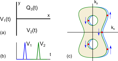
Figure 1: (a,b) A thought experiment in which $h/e$ voltage pulses are applied to regions 1 and 2 in (a). (c) shows a hypothetical 2D Fermi sea with $\chi_{F}=-1$. After pulse $V_{1}(t)$ for $x>0$ there are extra electrons (shown in blue) propagating to the right. Pulse $V_{2}(t)$ accelerates those electrons, and $v_{y}$ changes sign at the points indicated by the red dots in a direction indicated by the arrows. The net excess charge in region 3 is determined by the difference between the number of concave and convex critical points on the Fermi surface with ${\bf v}_{\bf k}\propto+\hat{x}$, which measures $\chi_{F}$.

It is simplest to consider the geometry in Fig. 1a, where region 1 is the half-plane $x<0$, and regions 2 (3) are the quadrants $x>0$, $y<0$($y>0$). In that case, the $V_{1}(t)$ pulse accelerates electrons in the $x$ direction, so that for every value of $k_{y}$ on the Fermi surface there is one extra electron propagating to the right ($v_{x}>0$) for $x>0$, and one extra hole propagating to the left ($v_{x}<0$) for $x<0$. $Q_{3}$ will be determined by the effect of the $V_{2}(t)$ pulse on those extra electrons with $x>0$, which are accelerated in the $y$ direction. As in the 1D example discussed above, the transferred charge can be determined by counting those electrons that change directions at the critical points on the Fermi surface where $v_{x}>0$ and $v_{y}=0$. Referring to the hypothetical Fermi surface in Fig. 1c, these arise at the points indicated by the dots, which come in two varieties distinguished by whether the Fermi surface is concave (convex) with $\partial^{2}E/\partial k_{y}^{2}>0$($<0$). $Q_{3}$ is then $e$ times the sum over those critical points with signs ${\rm sgn}[\partial^{2}E/\partial k_{y}^{2}]$. By inspecting Fig. 1c, it is clear that this is $\chi_{F}$. This will be proven below. We conclude that $Q_{3}=e\chi_{F}$.

The above argument can be sharpened by developing a semi-classical Boltzmann transport theory. In the absence of scattering the electron distribution function $f({\bf k},{\bf r},t)$ satisfies the collisionless Boltzmann equation,

$$(\partial/\partial t+{\bf v}_{\bf k}\cdot\nabla_{\bf r}+e{\bf E}\cdot\nabla_{\bf k}/\hbar)f=0.$$ (5)

Consider two weak pulses, ${\bf E}_{1}(x_{1},y_{1},t)=\xi_{1}\delta(t-t_{1})\delta(x_{1})\hat{x}$ and ${\bf E}_{2}(x_{2},y_{2},t)=\xi_{2}\delta(t-t_{2})[\delta(y_{2})\theta(x_{2})\hat{y}-\delta(x_{2})\theta(-y_{2})\hat{x}]$. We compute the charge

$$Q_{3}(t_{3})=e\int\frac{d^{2}k}{(2\pi)^{2}}\int_{0}^{\infty}dx_{3}dy_{3}\delta f({\bf k},x_{3},y_{3},t_{3})$$ (6)

perturbatively at order $\xi_{1}\xi_{2}$ for $t_{1}<t_{2}<t_{3}$. Integrating (5) to this order gives $\delta f=e^{2}\xi_{1}\xi_{2}\delta\tilde{f}/\hbar^{2}$ with

$$\delta\tilde{f}=\int dy_{1}dx_{2}\delta({\bf r}_{32}-{\bf v}_{\bf k}t_{32})\frac{\partial}{\partial{k_{y}}}[\delta({\bf r}_{21}-{\bf v}_{{\bf k}}t_{21})\frac{\partial f_{0}}{\partial{k_{x}}}],$$ (7)

where $f_{0}({\bf k})=\theta(E_{F}-E({\bf k}))$, $t_{ij}=t_{i}-t_{j}$, ${\bf r}_{32}=(x_{3}-x_{2},y_{3})$, ${\bf r}_{21}=(x_{2},-y_{1})$, and $x_{2}$ ($y_{1}$) are integrated from $0$ ($-\infty$) to $\infty$. The second term in ${\bf E}_{2}$, with $x_{2}=0$, is absent because the $\delta$ functions can not be satisfied. After plugging (7) into (6), the four spatial integrals cancel the $\delta$ functions, but since $x_{2}>0$ ($y_{3}>0$), we require $v_{x}>0$ ($v_{y}>0$) inside (outside) $\partial/\partial k_{y}$. After integrating by parts on $k_{y}$ and replacing $\xi_{1,2}\rightarrow h/e$ we obtain

$$Q_{3}=-e\int d^{2}k\frac{\partial f_{0}({\bf k})}{\partial k_{x}}\theta(v_{x}({\bf k}))\frac{\partial\theta(v_{y}({\bf k}))}{\partial k_{y}}.$$ (8)

This captures the result of the heuristic argument above: $-\partial f_{0}/\partial k_{x}$ isolates the Fermi surface, while $\theta(v_{x})\partial(\theta(v_{y}))/\partial k_{y}$ isolates the critical points on the Fermi surface identified in Fig. 1c. To make contact with Eq. 4, it is convenient to add zero to the integrand in the form $-(\partial f_{0}/\partial k_{y})\theta(v_{x})\partial\theta(v_{y})/\partial k_{x}$. This is clearly zero, since $\partial f_{0}/\partial k_{y}=v_{y}\partial f_{0}/\partial E$, and $\partial\theta(v_{y})/\partial k_{x}$ fixes $v_{y}=0$. This allows us to integrate by parts to obtain,

$$Q_{3}=e\int d^{2}kf_{0}({\bf k})[\frac{\partial\theta(v_{x})}{\partial k_{x}}\frac{\partial\theta(v_{y})}{\partial k_{y}}-\frac{\partial\theta(v_{x})}{\partial k_{y}}\frac{\partial\theta(v_{y})}{\partial k_{x}}]$$ (9)

The integrand is only non-zero near critical points where $v_{x}=v_{y}=0$. The integral evaluates the signature of each critical point, leading to

$$Q_{3}=e\sum_{m}\eta_{m}=e\chi_{F}.$$ (10)

We next consider the frequency domain response. This can be computed using the Boltzmann theory, however, we will first formulate a more general quantum non-linear response theory, and show the Boltzmann theory follows, provided the applied fields vary slowly in space and time. To this end, we introduce the Hamiltonian

$${\cal H}={\cal H}_{0}+(V_{1}\hat{Q}_{1}e^{(\eta-i\omega_{1})t}+V_{2}\hat{Q}_{2}e^{(\eta-i\omega_{2})t}+{\rm h.c.})$$ (11)

with ${\cal H}_{0}=\sum_{\bf k}E({\bf k})c_{\bf k}^{\dagger}c_{\bf k}$ and $\hat{Q}_{p}=\int d{\bf r}Q_{p}({\bf r})\rho({\bf r})$ is defined in terms of the density operator $\rho({\bf r})$ for each of the three regions in Fig. 1a. $Q_{p}({\bf r})$ is $1$ ($0$) inside (outside) region $p$ and is assumed to transition smoothly between $1$ and $0$ in a width $b$ near the boundary, with $k_{F}b\gg 1$.

Figure 2: Feynman diagrams for the conductance. (a,b) describe the 2D non-linear conductance and (c) describes the 1D linear conductance in the absence of interactions and give the quantized conductance determined by $\chi_{F}$. (d) and (e) show corrections to (a,b) and (c) that describe screening due to electron interactions and modify the quantized result.

We compute the charge $Q_{3}(t)$ at frequency $\omega_{1}+\omega_{2}$ to order $V_{1}V_{2}$. We adopt a scalar potential formulation, which avoids the diamagnetic term. The response has structure similar to second order nonlinear optical responseKraut and von Baltz (1979); von Baltz and Kraut (1981); Zhang et al. (2018), and is determined by evaluating the Feynman diagrams in Fig. 2a,b.

$$Q_{3}(\omega_{1}+\omega_{2})=\alpha(\omega_{1},\omega_{2})V_{1}V_{2}$$ (12)

with

$$\alpha(\omega_{1},\omega_{2})= \frac{e^{3}}{\hbar^{2}}\sum_{l,m,n}\frac{f_{l}-f_{m}}{\omega_{1}-\omega_{lm}+i\eta}[\frac{Q_{1}^{lm}Q_{2}^{mn}Q_{3}^{nl}}{\omega_{1}+\omega_{2}-\omega_{ln}+i\eta}$$

$$-\frac{Q_{1}^{lm}Q_{3}^{mn}Q_{2}^{nl}}{\omega_{1}+\omega_{2}-\omega_{nm}+i\eta}]+(1\leftrightarrow 2).$$ (13)

Here $l,m,n$ label momenta, $\omega_{lm}=(E({\bf k}_{l})-E({\bf k}_{m}))/\hbar$, $f_{l}=f_{0}({\bf k}_{l})$ is a Fermi function, and

$$Q_{p}^{lm}=\langle{\bf k}_{l}|\hat{Q}_{p}|{\bf k}_{m}\rangle=\int d{\bf r}_{p}Q_{p}({\bf r}_{p})e^{i{\bf q}_{lm}\cdot{\bf r}_{p}}$$ (14)

with ${\bf q}_{lm}={\bf k}_{l}-{\bf k}_{m}$. Since $Q_{p}({\bf r})$ varies on the scale of $b$, an expansion in ${\bf q}_{lm}$ and ${\bf q}_{nm}$ is justified. As shown in supplemental section A, the ${\bf q}_{lm}$ and ${\bf q}_{nm}$ integrals can be performed to obtain,

$$\alpha= \int\frac{d^{2}{\bf k}d^{6}{\bf r}_{1,2,3}}{(2\pi)^{2}}\nabla^{a}_{\bf r}Q_{1}({\bf r}_{1})\nabla^{b}_{\bf r}Q_{2}({\bf r}_{2})Q_{3}({\bf r}_{3})[\nabla_{\bf k}^{a}f_{0}({\bf k})$$

$$D({\bf r}_{21},{\bf k},\omega_{1})\nabla_{\bf k}^{b}D({\bf r}_{32},{\bf k},\omega_{1}+\omega_{2})]+(1\leftrightarrow 2)$$ (15)

with $D({\bf r},{\bf k},\omega)=e^{-(\eta-i\omega)|{\bf r}|/|{\bf v}_{\bf k}|}\delta({\bf r}\times{\bf v}_{\bf k})\theta({\bf r}\cdot{\bf v}_{\bf k})$. This form of the response also follows from solving (5) in the frequency domain with ${\bf E}_{p}({\bf r},t)=-\nabla Q_{p}({\bf r})V_{p}e^{(\eta-i\omega_{p})t}$.

In supplemental section B, we evaluate (15) for the infinite plane in which three rays separate regions that subtend angles $\varphi_{p}$ (see Fig. 3). We show that there is an intrinsic term $\alpha_{i}(\omega_{1},\omega_{2})=\chi_{F}(e^{3}/h^{2})/(\eta-i\omega_{1})(\eta-i\omega_{2})$ that is independent $\varphi_{p}$ (provided all $\varphi_{p}<\pi$) as well as the detailed spatial profile of the fields. In addition, there is an extrinsic term with a distinct frequency dependence, $\alpha_{e}(\omega_{1},\omega_{2})=k(e^{3}/h^{2})/(\eta-i(\omega_{1}+\omega_{2}))^{2}$ with a coefficient $k$ that depends on $\varphi_{p}$ as well as the details of the Fermi surface. The extrinsic term was not picked up by the pulse argument (where we assumed $t_{2}>t_{1}$), since it arises when ${\bf E}_{1}$ and ${\bf E}_{2}$ coincide in time. The intrinsic term dominates when $\omega_{1}+\omega_{2}\gg\omega_{1}$ or $\omega_{2}$. The intrinsic term, which is exact for the infinite plane and non-interacting electrons is the central result of this paper. To address experimental feasibility we must consider the role of contacts as well as electron-electron interactions. These both introduce complications into the analysis.

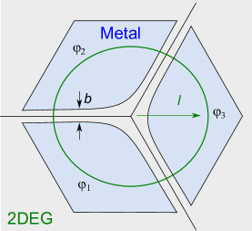
Figure 3: A triple point contact as a model experimental geometry. A 2D electron gas is connected to three metallic leads of size larger than the tunneling mean free path $\ell$. The leads are separated by $b$ and subtend angles $\varphi_{1,2,3}$.

As a model for electrical contacts, consider Fig. 3, which depicts a 2D electron gas (2DEG) of size $L$ with large area tunnel contacts to ideal metallic leads separated by a distance $b$. Provided the capacitance between the contacts and the 2DEG is sufficiently large, the voltages in the leads will establish a potential profile in the 2DEG as in Eq. 11. We assume the tunnel barrier is in a regime in which the mean free path $\ell$ for tunneling from the 2DEG to the leads satisfies $k_{F}^{-1}\ll\ell\ll L$. This defines a dwell time $\tau=\ell/v_{F}$ for electrons in the 2DEG. In the pulse construction, we clearly require $t_{21}<\tau$, since for $t_{21}>\tau$ the first pulse has disappeared before the second arrives. In the frequency domain calculation, tunneling to the leads introduces an exponential decay $e^{-|{\bf r}|/\ell}$ into $D({\bf r},{\bf k},\omega)$, which cuts off the small $\omega_{1}$ divergence in $\alpha$, effectively replacing $\omega_{1}\rightarrow\omega_{1}+i/\tau$. The coupling to the leads therefore places a lower bound $\omega_{1},\omega_{2}\gg\omega_{c}$ for the applicability of (2) with $\omega_{c}\sim\tau^{-1}$. The intrinsic behavior is thus recovered when $\omega_{c}\ll\omega_{1(2)}\ll\omega_{2(1)}$.

A second complication involves the role of electron-electron interactions. In 1D, the analog of our calculation is the Kubo formula conductance $G_{\rm Kubo}$, which is given by $G_{\rm Kubo}=Ke^{2}/h$, where $K<1$ is the Luttinger parameter characterizing repulsive electron interactionsApel and Rice (1982); Kane and Fisher (1992). However, $G_{\rm Kubo}$ does not correctly account for the electrical contacts, and it was argued that for Fermi liquid leads on a 1DEG of length $L$, $G(\omega)=e^{2}/h$ for $\omega\ll v_{F}/L$Maslov and Stone (1995); Ponomarenko (1995); Safi and Schulz (1995); Safi (1997, 1999); Thomale and Seidel (2011). An appealing interpretation of this was explained by KawabataKawabata (1996), who argued that $G_{\rm Kubo}$ computed in an infinite system is renormalized because it describes the response to the applied voltage, while the quantized conductance, which reflects the chiral anomaly, is the response to the self-consistent potential, which includes screening due to interactions. Moreover, for the DC conductance it is the self-consistent potential that determines the measured electrochemical potential difference. ShimizuShimizu (1996) emphasized the similarity of this description to Fermi liquid theoryPines and Nozieres (1966). In terms of Feynman diagrams, for the response to the applied field, the Kubo formula bubble diagram (Fig. 2(c)) is dressed by convolving with RPA-like polarization bubbles (Fig. 2(d)), $\Pi(x,\omega)$, represented here in real space. For a 1DEG in which leads are modeled by setting the interactions to zero for $|x|>L$, it can be checked that since $\Pi(x,\omega)\sim(\omega/v_{F})e^{i\omega x/v_{F}}$, and $|x|<L$ the interaction corrections vanish for $\omega\ll v_{F}/L$.

To incorporate electron interactions into the calculation of the 2D non-linear response we adopt a renormalized Fermi liquid descriptionShankar (1994) in which quasiparticles near $E_{F}$ interact with an energy $f_{{\bf k}{\bf k}^{\prime}}n_{\bf k}n_{{\bf k}^{\prime}}$, where $n_{\bf k}=c_{\bf k}^{\dagger}c_{\bf k}$. At low energy, the important interaction corrections involve RPA bubblesRostami et al. (2017), and summing the diagrams like 2(e) is equivalent to incorporating the Fermi liquid interactions $f_{{\bf k}{\bf k}^{\prime}}$ into the Boltzmann equationPines and Nozieres (1966); Shankar (1994). This is difficult to solve in general, but by evaluating the simplest diagram at first order in $f_{{\bf k}{\bf k^{\prime}}}$ it can be checked that the response to the applied field is modified: $\chi_{F}\rightarrow\chi_{F}+O(N(E_{F})f)$, where $f$ is an average of $f_{{\bf k}{\bf k}^{\prime}}$ over the Fermi surface. Thus, the non-linear response in 2D is modified by the Fermi liquid parameters just as the linear response in 1D is modified by the Luttinger parameter. The bubble $\Pi(\omega,{\bf r})\propto(\omega/v_{F})e^{i\omega|{\bf r}|/v_{F}}$ vanishes for $\omega\ll\omega_{c}$ as for $D=1$. However, since we must consider $\omega_{1},\omega_{2}\gg\omega_{c}$, the interaction corrections remain. The origin of the correction is the same as in $D=1$: due to interactions, the potential is screened, as is accounted for by the RPA bubbles.

At finite frequency, more detailed modeling is required to determine the relation between the self-consistent potential and the measured voltage. In the absence of that, it will be fruitful to consider weakly interacting systems. Consider a 2D Dirac material, such as graphene, with density of states $N(E)\sim|E|/v_{F}^{2}$. For a short ranged interaction (screened by the leads) $N(E_{F})f\ll 1$ for sufficiently small $E_{F}$. Interestingly, the Fermi surface is electron-like (hole-like) for $E_{F}>0$($E_{F}<0$), so the response characterized by $\chi_{F}=4{\rm sgn}E_{F}$ (including spin and valley) changes sign at charge neutrality.

Our analysis opens several avenues for further inquiry. On the practical side, it will be interesting to search for other measurable quantities that probe $\chi_{F}$. Promising candidates include low frequency current noise as well as thermal conductance. It will also be interesting to generalize our theory to $D>2$ and to explore ways in which $\chi_{F}$ provides a fundamental characterization of a degenerate Fermi gas. Our analysis suggests that $\chi_{F}$ defines a kind of “higher order” anomaly. In 1D, the chiral anomaly characterizes the connection between left and right moving electrons, which leads to a lack of conservation of the right movers. For $D>1$, $\chi_{F}$ characterizes a more general violation of conservation due to the fact that electrons propagating in different directions are connected at critical points ${\bf k}_{m}$. This is related to the Fermi surface anomaly discussed in Ref. Else et al., 2021, which characterizes a particular point on the Fermi surface. However, unlike that description, $\chi_{F}$ provides a global characterization of the Fermi surface. For $D=1$ the bipartite entanglement entropy has a universal term $S=(c/3){\rm log}L$Holzhey et al. (1994); Calabrese and Cardy (2004) with $c=\chi_{F}$. This has been generalized to higher $D$, where $S$ describes a logarithmic area law entanglement that involves the projected area of the Fermi surfaceGioev and Klich (2006); Swingle (2010), which is non-zero even for a system of decoupled 1D wiresDing et al. (2012), with $\chi_{F}=0$. We speculate that for $D>1$, $\chi_{F}$ shows up in an intrinsically $D$ dimensional entanglement measure.

We thank Patrick Lee and Pok Man Tam for helpful suggestions. This work was supported by a Simons Investigator Grant from the Simons Foundation.

Supplemental Material

Appendix A Non-linear response for slowly varying fields

In this section we evaluate the quantum non-linear response formula, Eq. 13 for potentials that vary slowly in space and time, and show that the result agrees with the perturbative solution of the Boltzmann equation, Eq. 5. In the slowly varying limit, all of the transitions in (13) will be intra-band, so a single band theory, characterized by dispersion $E({\bf k})$ will suffice.

Our starting point is to write Eq. 13 in real space.

$$\alpha(\omega_{1},\omega_{2})=\frac{e^{3}}{\hbar^{2}}\int d^{6}{\bf r}_{1,2,3}Q_{1}({\bf r}_{1})Q_{2}({\bf r}_{2})Q_{3}({\bf r}_{3})\chi(\left\{\omega_{p},{\bf r}_{p}\right\})$$ (16)

with

$$\chi(\left\{{\bf r}_{p},\omega_{p}\right\})=\sum_{{\bf k}_{l,m,n}}\frac{f_{l}-f_{m}}{\omega_{1}-\omega_{lm}+i\eta}[\frac{\rho_{lm}({\bf r}_{1})\rho_{mn}({\bf r}_{2})\rho_{nl}({\bf r}_{3})}{\omega_{1}+\omega_{2}-\omega_{ln}+2i\eta}-\frac{\rho_{lm}({\bf r}_{1})\rho_{mn}({\bf r}_{3})\rho_{nl}({\bf r}_{2})}{\omega_{1}+\omega_{2}-\omega_{nm}+2i\eta}]+(1\leftrightarrow 2).$$ (17)

When $Q_{p}({\bf r}_{p})$ is slowly varying, the matrix elements of the density operator will be dominated by intraband terms with small momenta, ${\bf q}_{lm}={\bf k}_{l}-{\bf k}_{m}\sim 1/b$,

$$\rho_{lm}({\bf r})=\langle{\bf k}_{l}|\rho({\bf r})|{\bf k}_{m}\rangle=e^{-i{\bf q}_{lm}\cdot{\bf r}}(1+O({\bf q}_{lm})).$$ (18)

Expanding to leading order in ${\bf q}_{lm}$ then gives

$$\chi(\left\{{\bf r}_{p},\omega_{p}\right\})=\sum_{{\bf k}_{l,n,m}}\frac{f_{l}-f_{m}}{\omega_{1}-{\bf q}_{lm}\cdot{\bf v}_{lm}+i\eta}[\frac{e^{i({\bf q}_{lm}\cdot{\bf r}_{31}+{\bf q}_{nm}\cdot{\bf r}_{32})}}{\omega_{1}+\omega_{2}-{\bf q}_{ln}\cdot{\bf v}_{ln}+2i\eta}-\frac{e^{i({\bf q}_{lm}\cdot{\bf r}_{31}+{\bf q}_{ln}\cdot{\bf r}_{32})}}{\omega_{1}+\omega_{2}-{\bf q}_{nm}\cdot{\bf v}_{nm}+2i\eta}]+(1\leftrightarrow 2)$$ (19)

where since it is necessary to keep order $q^{2}$ terms in the denominator we write $\omega_{lm}={\bf q}_{lm}\cdot{\bf v}_{lm}+O(q^{3})$, with ${\bf v}_{lm}={\bf v}_{({\bf k}_{l}+{\bf k}_{m})/2}$. If we define ${\bf k}=({\bf k}_{l}+{\bf k}_{m})/2$, then ${\bf v}_{lm}={\bf v}_{\bf k}$, ${\bf v}_{ln}={\bf v}_{{\bf k}+{\bf q}_{nm}/2}$ and ${\bf v}_{nm}={\bf v}_{{\bf k}-{\bf q}_{ln}/2}$. We next define ${\bf q}_{1}={\bf q}_{lm}$ and ${\bf q}_{2}={\bf q}_{mn}$ (${\bf q}_{ln}$) in the first (second) term. It follows that

$$\chi(\left\{{\bf r}_{p},\omega_{p}\right\})= \sum_{{\bf k},{\bf q}_{1},{\bf q}_{2}}e^{i({\bf q}_{1}\cdot{\bf r}_{31}+{\bf q}_{2}\cdot{\bf r}_{32})}\frac{f({\bf k}+{\bf q}_{1}/2)-f({\bf k}-{\bf q}_{1}/2)}{\omega_{1}-{\bf q}_{1}\cdot{\bf v}_{\bf k}+i\eta}$$

$$[\frac{1}{\omega_{1}+\omega_{2}-({\bf q}_{1}+{\bf q}_{2})\cdot{\bf v}_{{\bf k}-{\bf q}_{2}/2}+2i\eta}-\frac{1}{\omega_{1}+\omega_{2}-({\bf q}_{1}+{\bf q}_{2})\cdot{\bf v}_{{\bf k}+{\bf q}_{2}/2}+2i\eta}]+(1\leftrightarrow 2)$$ (20)

$$= -\sum_{{\bf k},{\bf q}_{1},{\bf q}_{2}}e^{i({\bf q}_{1}\cdot{\bf r}_{31}+{\bf q}_{2}\cdot{\bf r}_{32})}\frac{{\bf q}_{1}\cdot\nabla_{\bf k}f({\bf k})}{\omega_{1}-{\bf q}_{1}\cdot{\bf v}_{\bf k}+i\eta}{\bf q}_{2}\cdot\nabla_{\bf k}\frac{1}{\omega_{1}+\omega_{2}-({\bf q}_{1}+{\bf q}_{2})\cdot{\bf v}_{{\bf k}}+2i\eta}+(1\leftrightarrow 2)$$ (21)

$$= \nabla^{a}_{{\bf r}_{1}}\nabla^{b}_{{\bf r}_{2}}\sum_{{\bf k},{\bf q}_{1},{\bf q}_{2}}e^{i({\bf q}_{1}\cdot{\bf r}_{31}+{\bf q}_{2}\cdot{\bf r}_{32})}\frac{\nabla_{\bf k}^{a}f({\bf k})}{\omega_{1}-{\bf q}_{1}\cdot{\bf v}_{\bf k}+i\eta}\nabla_{\bf k}^{b}\frac{1}{\omega_{1}+\omega_{2}-({\bf q}_{1}+{\bf q}_{2})\cdot{\bf v}_{{\bf k}}+2i\eta}+(1\leftrightarrow 2)$$ (22)

Now we can do the sums over ${\bf q}_{1}$ and ${\bf q}_{2}$ using independent variables ${\bf q}_{1}$ and ${\bf q}_{3}=-{\bf q}_{1}-{\bf q}_{2}$. Let us define

$$D({\bf r},\omega,{\bf v})=i\sum_{\bf q}\frac{e^{i{\bf q}\cdot{\bf r}}}{\omega-{\bf q}\cdot{\bf v}+i\eta}=\frac{e^{(i\omega-\eta)|{\bf r}|/|{\bf v}|}}{|{\bf v}|}\delta(\hat{\bf v}\times{\bf r})\theta(\hat{\bf v}\cdot{\bf r})$$ (23)

Then

$$\chi(\left\{{\bf r}_{p},\omega_{p}\right\})=-\nabla^{a}_{{\bf r}_{1}}\nabla^{b}_{{\bf r}_{2}}\sum_{{\bf k}}(\nabla^{a}_{\bf k}f({\bf k}))D({\bf r}_{21},\omega_{1},{\bf v}_{\bf k})\nabla^{b}_{\bf k}D({\bf r}_{32},\omega_{1}+\omega_{2},{\bf v}_{\bf k})+(1\leftrightarrow 2)$$ (24)

Plugging (24) into (16) reproduces Eq. 15 in the main text. Note, that the same result would follow by integrating the Boltzmann equation (Eq. 5) to order $V_{1}V_{2}$, with ${\bf E}_{p=1,2}({\bf r},t)=-\nabla Q_{p}({\bf r})V_{p}e^{(\eta-i\omega_{p})t}$.

Appendix B Non-linear response for a triple point contact

In this appendix we evaluate the non-linear response in the frequency domain described by Eq. 15 for a triple point contact, depicted in Fig. B1 in which the three contact regions meet at a point and subtend arbitrary angles $\varphi_{p=1,2,3}$. We will show that the non-linear response function consists of two terms with distinct frequency dependences. There is an intrinsic term of the form,

$$\alpha_{i}(\omega_{1},\omega_{2})=\chi_{F}\frac{e^{3}}{h^{2}}\frac{1}{(\eta-i\omega_{1})(\eta-i\omega_{2})}$$ (25)

which depends only on the Euler characteristic of the Fermi sea and is insensitive to $\varphi_{p}$, provided all three angles satisfy $\varphi_{p}<\pi$. This generalizes the analysis of Eqs. 5-10 to the frequency domain and to a more general geometry. At the end we will show how this result is modified when one of the contact angles is greater than $\pi$. In addition, there is an extrinsic term,

$$\alpha_{e}(\omega_{1},\omega_{2})=k\frac{e^{3}}{h^{2}}\frac{1}{(\eta-i(\omega_{1}+\omega_{2}))^{2}}$$ (26)

where $k$ is a dimensionless constant that depends on the details of the Fermi surface, as well as the angles $\varphi_{p}$. An explicit formula for $k$ will be given below.

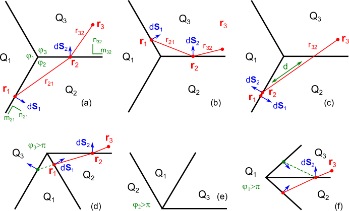
Figure B1: A triple point contact with three contact regions that meet at a point and subtend arbitrary angles $\varphi_{1,2,3}$. (a,b,c) show three contributions to $\alpha_{1}(\omega_{1},\omega_{2})$ for the case all angles $\varphi_{p}<\pi$. (a) and (b) contribute to the intrinsic term, while (c) contributes to the extrinsic term. (d,e,f) show contributions to the intrinsic term in the cases where one of the angles is greater than $\pi$. For (d) and (e) the contribution is zero, while for (f) it is the same as (a) and (b).

We assume the region boundaries, where $\nabla Q_{p}({\bf r})$ is non-zero, are confined a region of width $b$ about the straight rays shown in Fig. B1. The slowly varying condition is satisfied provided $k_{F}b\gg 1$. Provided $\omega b\ll 1$, the result will be independent of $b$. Due to the gradients on $Q_{p}({\bf r}_{p})$ for $p=1,2$ in Eq. 15, ${\bf r}_{p=1,2}$ are confined to the boundary of region $p$. We thus evaluate

$$\alpha(\omega_{1},\omega_{2})=\alpha_{1}(\omega_{1},\omega_{2})+\alpha_{2}(\omega_{1},\omega_{2})$$ (27)

with

$$\alpha_{1}(\omega_{1},\omega_{2})=\frac{e^{3}}{\hbar^{2}}\sum_{\bf k}\int d{\bf S}^{a}_{1}d{\bf S}^{b}_{2}d^{2}{\bf r}_{3}(\nabla_{\bf k}^{a}f({\bf k}))D({\bf r}_{21},{\bf k},\omega_{1})\nabla_{\bf k}^{b}D({\bf r}_{32},{\bf k},\omega_{1}+\omega_{2})$$ (28)

where ${\bf r}_{p=1,2}$ are integrated along the boundary of region $p$, with the perpendicular length element $d{\bf S}_{p}$ pointing away from region $p$. $\alpha_{2}$ is obtained by interchanging $1\leftrightarrow 2$. It is convenient to write 23 as

$$D({\bf r},{\bf k},\omega)=\int_{0}^{\infty}dte^{i\omega t}\delta^{2}({\bf r}-{\bf v}_{\bf k}t).$$ (29)

We then obtain

$$\alpha_{1}(\omega_{1},\omega_{2})=\frac{e^{3}}{\hbar^{2}}\int_{0}^{\infty}dt_{21}dt_{32}e^{i\omega_{1}t_{21}+i(\omega_{1}+\omega_{2})t_{32}}\int d{\bf S}^{a}_{1}d{\bf S}^{b}_{2}d^{2}{\bf r}_{3}\sum_{\bf k}(\nabla_{\bf k}^{a}f({\bf k}))\delta^{2}({\bf r}_{21}-{\bf v}_{\bf k}t_{21})\nabla_{\bf k}^{b}\delta^{2}({\bf r}_{32}-{\bf v}_{\bf k}t_{32}).$$ (30)

This shows that the integrals are dominated by straight lines parallel to ${\bf v}_{\bf k}$ that begin on ${\bf r}_{1(2)}$ on the boundary of region 1(2) and end on ${\bf r}_{3}$ in the interior of region 3, while visiting ${\bf r}_{2(1)}$ on the boundary of region 2(1) along the way. Due to the derivative $\nabla_{\bf k}^{b}$ in (30) the two segments of the line should be considered to have slightly different slopes. This is important when ${\bf v}_{\bf k}$ is parallel to one of the boundaries.

There are three contributions to $\alpha_{1}$: $\alpha_{1A,1B,1C}$, shown in panels (a,b,c) of Fig. B1, that depend on which segments of the boundaries ${\bf r}_{1}$ and ${\bf r}_{2}$ are on. (A fourth combination is not present because a straight line ${\bf r}_{1}\rightarrow{\bf r}_{2}\rightarrow{\bf r}_{3}$ can not be formed.) We will see that the intrinsic term is $\alpha_{i}=\alpha_{1A}+\alpha_{1B}+\alpha_{2A}+\alpha_{2B}$ and the extrinsic term is $\alpha_{e}=\alpha_{1C}+\alpha_{2C}$.

We parameterize the boundary ray separating region $p$ and region $q$ by writing ${\bf r}_{p}=z_{p}\hat{m}_{qp}$, where $0<z_{p}<\infty$ and $\hat{m}_{pq}\equiv\hat{m}_{qp}$ is a unit vector pointing along the ray. The perpendicular length element is given by $d{\bf S}_{p}=dz_{p}\hat{n}_{pq}$, where $\hat{n}_{qp}\equiv-\hat{n}_{pq}$ is a unit vector perpendicular to $\hat{m}_{pq}$ pointing away from region $p$.

B.1 Intrinsic Terms

For $\alpha_{1A}(\omega_{1},\omega_{2})$ (Fig. B1a), the integral over ${\bf r}_{3}$ can be evaluated using

$$\int d^{2}{\bf r}_{3}\delta^{2}({\bf r}_{3}-z_{32}\hat{m}_{32}-{\bf v}_{\bf k}t_{32})=\theta({\bf v}_{\bf k}\cdot\hat{n}_{32}),$$ (31)

where we note that $t_{32}>0$. The integral over ${\bf r}_{1,2}$ follows from

$$\int_{0}^{\infty}dz_{1}dz_{2}\delta^{2}(z_{2}\hat{m}_{32}-z_{1}\hat{m}_{21}-{\bf v}_{\bf k}t_{21})=\frac{\theta({\bf v}_{\bf k}\cdot\hat{n}_{21})\theta({\bf v}_{\bf k}\cdot\hat{n}_{32})}{|\hat{m}_{32}\times\hat{m}_{21}|}.$$ (32)

We then find

$$\alpha_{1A}(\omega_{1},\omega_{2})=\frac{e^{3}}{\hbar^{2}}\int_{0}^{\infty}dt_{21}dt_{32}e^{i\omega_{1}t_{21}+i(\omega_{1}+\omega_{2})t_{32}}\sum_{\bf k}(\hat{n}_{21}\cdot\nabla_{\bf k}f({\bf k}))\frac{\theta({\bf v}_{\bf k}\cdot\hat{n}_{21})\theta({\bf v}_{\bf k}\cdot\hat{n}_{32})}{|\hat{m}_{32}\times\hat{m}_{21}|}\hat{n}_{32}\cdot\nabla_{\bf k}\theta({\bf v}_{\bf k}\cdot\hat{n}_{32})$$ (33)

Since $\nabla_{\bf k}\theta({\bf v}_{\bf k}\cdot\hat{n}_{32})$ fixes ${\bf v}_{\bf k}\parallel\hat{m}_{32}$, and $\nabla_{\bf k}f({\bf k})\parallel{\bf v}_{\bf k}$ we can write $\hat{n}_{21}\cdot\nabla_{\bf k}f({\bf k})=(\hat{n}_{21}\cdot\hat{m}_{32})\hat{m}_{32}\cdot\nabla_{\bf k}f({\bf k})$, along with $\theta({\bf v}_{\bf k}\cdot\hat{n}_{21})=\theta({\bf v}_{\bf k}\cdot m_{32})$. Since $\hat{n}_{21}=\hat{z}\times\hat{m}_{21}$, $\hat{n}_{21}\cdot\hat{m}_{32}/|\hat{m}_{32}\times\hat{m}_{21}|=1$, and we obtain,

$$\alpha_{1A}(\omega_{1},\omega_{2})=\frac{e^{3}/\hbar^{2}}{(\eta-i(\omega_{1}+\omega_{2}))(\eta-i\omega_{1})}\sum_{\bf k}(\hat{m}_{32}\cdot\nabla_{\bf k}f({\bf k}))\theta(\hat{m}_{32}\cdot{\bf v}_{\bf k})\theta(\hat{n}_{32}\cdot{\bf v}_{\bf k})\hat{n}_{32}\cdot\nabla_{\bf k}\theta({\bf v}_{\bf k}\cdot\hat{n}_{32})$$ (34)

The analysis of $\alpha_{1B}(\omega_{1},\omega_{2})$ is almost the same. The only difference is that in (32) $\theta({\bf v}_{\bf k}\cdot\hat{n}_{32})$ is replaced by $\theta(-{\bf v}_{\bf k}\cdot\hat{n}_{32})$. For $\alpha_{1A}+\alpha_{1B}$ we can use $\theta(x)+\theta(-x)=1$. After adding a similar contributions to $\alpha_{2A}+\alpha_{2B}$ we obtain the intrinsic term in the non-linear response

$$\alpha_{i}(\omega_{1},\omega_{2})=\frac{e^{3}/\hbar^{2}}{(\eta-i(\omega_{1}+\omega_{2}))(\eta-i\omega_{1})}\sum_{\bf k}(\hat{m}_{32}\cdot\nabla_{\bf k}f({\bf k}))\theta(\hat{m}_{32}\cdot{\bf v}_{\bf k})\hat{n}_{32}\cdot\nabla_{\bf k}\theta({\bf v}_{\bf k}\cdot\hat{n}_{32})+(1\leftrightarrow 2)$$ (35)

Following the analysis of Eq. 8, the sum on ${\bf k}$ gives $\chi_{F}/(2\pi)^{2}$, and combining the two frequency dependent terms leads to (25)

We next consider the contributions to $\alpha_{i}$ in the case where one of the angles $\varphi_{p}$ is greater than $\pi$. The case $\alpha_{3}>\pi$ is shown in Fig B1a. In that case the contributions due to the two boundaries of region 1 (indicated by the red and green dots) have opposite sign due to the opposite projections of $d{\bf S}_{1}$ onto ${\bf v}_{\bf k}$, and in fact, they exactly cancel: $\alpha_{1A}+\alpha_{1B}=0$. In the case $\alpha_{2}>\pi$, shown in Fig. B1b, there are no contributions, since there are straight lines visiting regions $1\rightarrow 2\rightarrow 3$, so again, $\alpha_{1A}+\alpha_{1B}=0$. On the other hand, when $\varphi_{1}>\pi$, shown in Fig. B1c, the contributions from the two boundaries of region 1 have the same sign, and the analysis is identical to the analysis when $\varphi_{1}<\pi$.

Combining these results, along with corresponding results for $\alpha_{2A}+\alpha_{2B}$, the general formula for the intrinsic term is,

$$\alpha_{i}(\omega_{1},\omega_{2})=\frac{\chi_{F}e^{3}/h^{2}}{2\eta-i(\omega_{1}+\omega_{2})}\left[\frac{\xi_{2}\xi_{3}}{\eta-i\omega_{1}}+\frac{\xi_{1}\xi_{3}}{\eta-i\omega_{2}}\right]$$ (36)

where

$$\xi_{p}=\left\{\begin{array}[]{ll}1&\varphi_{p}<\pi\\ 0&\varphi_{p}>\pi\end{array}\right.$$ (37)

For the case where all angles are less than $\pi$ we recover Eq. 1. Note that for the special case treated in Eq. 6-10, with $\varphi_{1}=\pi$, when the $V_{2}$ pulse follows the $V_{1}$ pulse, the excess charge $Q_{3}$ depends only on the first term in the brackets of (36), and is insensitive to $\varphi_{1}=\pi$.

B.2 Extrinsic Terms

We now consider the contribution $\alpha_{1C}$ from Fig. B1c. This term did not show up in the time-domain pulse argument presented in the main text because there we assumed that $t_{2}>t_{1}$, so the ${\bf E}_{1}$ and ${\bf E}_{2}$ pulses were separated in time. The frequency domain response, however, also includes a contribution from $t_{1}\sim t_{2}$. For the $\alpha_{1C}$ term, ${\bf r}_{1}\sim{\bf r}_{2}$, so $t_{1}\sim t_{2}$. This leads to an extrinsic contribution that depends on the angles $\varphi_{p}$ as well as the shape of the Fermi surface, but has a distinct frequency dependence from the intrinsic term.

The integral over ${\bf r}_{3}$ gives,

$$\int d^{2}{\bf r}_{3}\delta^{2}({\bf r}_{3}-z_{2}\hat{m}_{21}-{\bf v}_{\bf k}t_{32})=\theta({\bf v}_{\bf k}\cdot\hat{n}_{32})\theta(t_{32}-t_{0}(z_{2}))$$ (38)

where the lower bound on $t_{32}$ is determined by the length $d$ of the segment in region 2,

$$t_{0}(z_{2})=\frac{d}{|{\bf v}_{\bf k}|}=z_{2}\frac{|\hat{m}_{21}\times\hat{m}_{32}|}{{\bf v}_{\bf k}\cdot\hat{n}_{32}}$$ (39)

It is then useful to integrate the other $\delta$ function over $z_{1}$ and $t_{21}$:

$$\int dz_{1}dt_{21}\delta^{2}((z_{2}-z_{1})\hat{m}_{21}-{\bf v}_{\bf k}t_{21})=\frac{\theta({\bf v}_{\bf k}\cdot\hat{n}_{21})}{|\hat{m}_{21}\times{\bf v}_{\bf k}|}.$$ (40)

This fixes $t_{21}=0$. Expressing the remaining integral over $z_{2}$ as an integral over $t_{0}=z_{2}|\hat{m}_{21}\times\hat{m}_{32}|/{\bf v}_{\bf k}\cdot\hat{n}_{32}$ we find

$$\alpha_{1C}(\omega_{1},\omega_{2})=\frac{e^{3}}{\hbar^{2}}\int_{0}^{\infty}dt_{0}\int_{t_{0}}^{\infty}dt_{32}e^{i(\omega_{1}+\omega_{2})t_{32}}\sum_{\bf k}(\hat{n}_{21}\cdot\nabla_{\bf k}f({\bf k}))\frac{\theta({\bf v}_{\bf k}\cdot\hat{n}_{21})}{|\hat{m}_{21}\times{\bf v}_{\bf k}|}\hat{n}_{12}\cdot\nabla_{\bf k}\frac{{\bf v}_{\bf k}\cdot\hat{n}_{32}\theta({\bf v}_{\bf k}\cdot\hat{n}_{32})}{|\hat{m}_{21}\times\hat{m}_{32}|}.$$ (41)

Noting that $\nabla_{\bf k}f({\bf k})=-{\bf v}_{\bf k}\delta(E_{\bf k})$, $\hat{n}_{12}=-\hat{n}_{21}$ and $\hat{n}_{21}\cdot{\bf v}_{\bf k}/||\hat{m}_{21}\times{\bf v}_{\bf k}|=1$ this becomes

$$\alpha_{1C}(\omega_{1},\omega_{2})=\frac{e^{3}}{\hbar^{2}}\frac{1}{(\eta-i(\omega_{1}+\omega_{2}))^{2}}\sum_{\bf k}\delta(E_{\bf k})\theta({\bf v}_{\bf k}\cdot\hat{n}_{21})\theta({\bf v}_{\bf k}\cdot\hat{n}_{32})\frac{(\hat{n}_{21}\cdot\nabla_{\bf k})(\hat{n}_{32}\cdot\nabla_{\bf k})E_{\bf k}}{|\hat{n}_{21}\times\hat{n}_{32}|}.$$ (42)

Combining this with the corresponding term for $\alpha_{2C}$ leads to Eq. 26, with the dimensionless constant $k$ given by

$$k=\int d^{2}{\bf k}\delta(E_{\bf k})\left[\theta({\bf v}_{\bf k}\cdot\hat{n}_{21})\theta({\bf v}_{\bf k}\cdot\hat{n}_{32})\frac{(\hat{n}_{21}\cdot\nabla_{\bf k})(\hat{n}_{32}\cdot\nabla_{\bf k})E_{\bf k}}{|\hat{n}_{21}\times\hat{n}_{32}|}+\theta({\bf v}_{\bf k}\cdot\hat{n}_{12})\theta({\bf v}_{\bf k}\cdot\hat{n}_{31})\frac{(\hat{n}_{12}\cdot\nabla_{\bf k})(\hat{n}_{31}\cdot\nabla_{\bf k})E_{\bf k}}{|\hat{n}_{12}\times\hat{n}_{31}|}\right]$$ (43)

$k$ involves an integral over the segment of the Fermi surface that has a velocity that points into region 3, and depends on the specific shape of the Fermi surface.

References

Klitzing et al. (1980)K. v. Klitzing, G. Dorda, and M. Pepper, “New method for high-accuracy
determination of the fine-structure constant based on quantized hall
resistance,” Phys. Rev. Lett. 45, 494–497 (1980).
Thouless et al. (1982)D. J. Thouless, M. Kohmoto,
M. P. Nightingale, and M. den Nijs, “Quantized hall conductance in a
two-dimensional periodic potential,” Phys.
Rev. Lett. 49, 405–408
(1982).
Haldane (2004)F. D. M. Haldane, “Berry curvature on the fermi surface: Anomalous hall effect as a topological
fermi-liquid property,” Phys. Rev. Lett. 93, 206602 (2004).
de Juan et al. (2017)F. de Juan, A.G. Grushin,
T. Morimoto, and J. E. Moore, “Quantized circular photogalvanic effect
in weyl semimetals,” Nature Communications 8, 15995 (2017).
Avdoshkin et al. (2020)Alexander Avdoshkin, Vladyslav Kozii, and Joel E. Moore, “Interactions remove the quantization of the chiral photocurrent at weyl
points,” Phys. Rev. Lett. 124, 196603 (2020).
Ashcroft and Mermin (1976)N. W. Ashcroft and N. D. Mermin, Solid State
Physics (Holt-Saunders, 1976).
Lifshitz (1960)I. M. Lifshitz, “Anomalies of
electron characteristics of a metal in the high pressure region,” Soviet Physics
JETP 11, 1130–1135
(1960).
Fisher and Lee (1981)Daniel S. Fisher and Patrick A. Lee, “Relation between conductivity and transmission matrix,” Phys.
Rev. B 23, 6851–6854
(1981).
van Wees et al. (1988)B. J. van Wees, H. van
Houten, C. W. J. Beenakker, J. G. Williamson, L. P. Kouwenhoven, D. van der
Marel, and C. T. Foxon, “Quantized
conductance of point contacts in a two-dimensional electron gas,” Phys. Rev. Lett. 60, 848–850 (1988).
van Weperen et al. (2013)Ilse van Weperen, Sébastien R. Plissard, Erik P. A. M. Bakkers, Sergey M. Frolov, and Leo P. Kouwenhoven, “Quantized conductance in an insb nanowire,” Nano Letters 13, 387–391 (2013).
Frank et al. (1998)Stefan Frank, Philippe Poncharal, Z. L. Wang,
and Walt A. de Heer, “Carbon nanotube quantum
resistors,” Science 280, 1744–1746 (1998).
Nakahara (1990)Mikio Nakahara, Geometry, topology and physics, Graduate student series in
physics (Hilger, Bristol, 1990).
Kraut and von
Baltz (1979)Wolfgang Kraut and Ralph von Baltz, “Anomalous bulk photovoltaic effect in ferroelectrics: A quadratic response
theory,” Phys. Rev. B 19, 1548–1554 (1979).
von Baltz and Kraut (1981)Ralph von Baltz and Wolfgang Kraut, “Theory of the
bulk photovoltaic effect in pure crystals,” Phys.
Rev. B 23, 5590–5596
(1981).
Zhang et al. (2018)Yang Zhang, Hiroaki Ishizuka, Jeroen van den
Brink, Claudia Felser,
Binghai Yan, and Naoto Nagaosa, “Photogalvanic effect in weyl
semimetals from first principles,” Phys.
Rev. B 97, 241118
(2018).
Note (1)If one of the angles is greater than ,
is still quantized, but its value is modified. See supplemental
section B, where it is also established that for Fig. 1a the
pulse argument analysis remains valid.
Apel and Rice (1982)W. Apel and T. M. Rice, “Combined effect of
disorder and interaction on the conductance of a one-dimensional fermion
system,” Phys. Rev. B 26, 7063–7065 (1982).
Maslov and Stone (1995)Dmitrii L. Maslov and Michael Stone, “Landauer conductance of luttinger liquids with leads,” Phys.
Rev. B 52, R5539–R5542
(1995).
Ponomarenko (1995)V. V. Ponomarenko, “Renormalization of the one-dimensional conductance in the luttinger-liquid
model,” Phys. Rev. B 52, R8666–R8667 (1995).
Safi and Schulz (1995)I. Safi and H. J. Schulz, “Transport in an
inhomogeneous interacting one-dimensional system,” Phys.
Rev. B 52, R17040–R17043 (1995).
Thomale and Seidel (2011)Ronny Thomale and Alexander Seidel, “Minimal model of
quantized conductance in interacting ballistic quantum wires,” Phys. Rev. B 83, 115330 (2011).
Rostami et al. (2017)Habib Rostami, Mikhail I. Katsnelson, and Marco Polini, “Theory of
plasmonic effects in nonlinear optics: The case of graphene,” Phys. Rev. B 95, 035416 (2017).
Else et al. (2021)Dominic V. Else, Ryan Thorngren, and T. Senthil, “Non-fermi
liquids as ersatz fermi liquids: General constraints on compressible
metals,” Phys. Rev. X 11, 021005 (2021).
Holzhey et al. (1994)Christoph Holzhey, Finn Larsen, and Frank Wilczek, “Geometric and renormalized entropy in conformal field theory,” Nuclear Physics B 424, 443–467 (1994).
Gioev and Klich (2006)Dimitri Gioev and Israel Klich, “Entanglement
entropy of fermions in any dimension and the widom conjecture,” Phys. Rev. Lett. 96, 100503 (2006).
Ding et al. (2012)Wenxin Ding, Alexander Seidel, and Kun Yang, “Entanglement
entropy of fermi liquids via multidimensional bosonization,” Phys. Rev. X 2, 011012 (2012).