An Optimal Transport Approach to Causal Inference

Abstract

We propose a method based on optimal transport theory for causal inference in classical treatment and control study designs. Our approach sheds a new light on existing approaches and generalizes them to settings with high-dimensional data. The implementation of our method leverages recent advances in computational optimal transport to produce an estimate of high-dimensional counterfactual outcomes. The benefits of this extension are demonstrated both on synthetic and real data that are beyond the reach of existing methods. In particular, we revisit the classical Card & Krueger dataset on the effect of a minimum wage increase on employment in fast food restaurants and obtain new insights about the impact of raising the minimum wage on employment of full- and part-time workers in the fast food industry.

1 Introduction

Causal inference is a central question behind data-driven decision making across a wide variety of domains such as health care, economics, marketing, education, law (Angrist and Pischke, 2008; Ho and Rubin, 2011; Imbens and Rubin, 2015; Rothman and Greenland, 2005), and, more recently, the life sciences (Bates et al., 2020; Belyaeva et al., 2021; Meinshausen et al., 2016; Squires et al., 2020).

One of the main promises of causal inference is to be able to answer the question “what if?”: What if a patient had received a different treatment? What if a stimulus check was for a different amount? What if this gene was knocked down? What if this photo was taken at night? These questions pertain to a hypothetical reality called a counterfactual. This powerful concept is behind most of the methods based on the theory of potential outcomes (Neyman, 1923; Rubin, 1974, 1978) currently employed across social and biomedical sciences (Rothman and Greenland, 2005; Morgan and Winship, 2014; Imbens and Rubin, 2015). If counterfactuals could be observed, the causal inference question would be trivial: the causal effect would simply be the difference between an observation and its counterfactual. In practice, however, counterfactuals cannot be observed; this limitation has been dubbed the “fundamental problem of causal inference” (Holland, 1986; Imbens and Rubin, 2015). In this context, the power of a causal inference method hinges on adequate modeling and estimation of counterfactuals. The goal of this paper is to propose a new modeling paradigm for counterfactuals that is based on optimal transport. As a byproduct, we leverage recent progress in the theory of statistical optimal transport to develop an estimation strategy for these counterfacturals and hence, causal effects.

We focus on the simpler case of two possible realities: with and without intervention. Consider a framework with four groups, that may not contain the same individuals: a treatment group pre-intervention, a treatment group post-intervention, a control group pre-intervention, and a control group post-intervention. The purpose of the control group is to quantify the natural drift, i.e., the time trends between the pre and post-intervention periods and that are not related to the intervention under study. In turn, the causal effect of an intervention, a.k.a treatment effect, is given by the change observed in the treatment group between the two periods, net of the natural drift.

Prior work. The two main existing methods for estimating causal effects in the above setting are the classical method of Difference-in-Differences (DiD) (Lechner, 2011; Wing et al., 2018) and its generalization beyond average and aggregate effects, the Changes-in-Changes (CiC) estimator (Athey and Imbens, 2006).

DiD is a linear approach designed to estimate average (or aggregate) causal effects (Abadie, 2005; Heckman, 1990) over all units. This method can be proved to correctly identify counterfactuals under the “parallel trends” assumption (Abadie, 2005; Ryan et al., 2019) under which the average natural shift is assumed to be the same across both the control and treatment group. This idea has been used in many areas of science where capturing the average treatment effect is sufficient to formulate informative causal conclusions. Impactful applications include quantifying the effect of public health measures in response to COVID-19 (Goodman-Bacon and Marcus, 2020) and estimating how irrigation farmers adapt to water quotas (Drysdale and Hendricks, 2018).

The fact that the linear DiD estimator only provides estimates of average and aggregate treatment is a severe limitation in many settings where treatment heterogeneity is important, i.e., where different units can react differently to the same intervention. The CiC estimator (Athey and Imbens, 2006) addresses this issue for univariate outcomes. It generalizes the DiD estimator by not just focusing on averages but the whole probability distribution of the respective units. This development permits the estimation of the entire counterfactual law of the fraction of treated units had they not received the treatment, hence allowing for a general form of heterogeneity in their response to treatment.

In its current form the CiC estimator is only applicable in settings with univariate outcomes, as it relies heavily on the definition of quantile functions. This makes it rather restrictive for modern applications where the outcomes of interest are often high-dimensional. This includes, for example A/B testing in digital marketing campaigns where outcomes are a combination of features such as click-through rate, time-per-page, etc., as well as measuring intervention effects such as gene knock down on a population of cells measured in high-dimensional gene space. In principle, the CiC estimator may be tensorized by estimating treatment effects independently for each coordinate but this solution fails to capture correlations that are often important in causal discovery.

Our contributions. We recast the CiC estimator using tools from the theory of optimal transport. This perspective allows us to extend this methodology to handle multivariate observables. Our approach relies on a natural extension of the causal model proposed in Athey and Imbens (2006) which guarantees that both populations, treatment and control, evolve between pre- and post-treatment periods via optimal transport maps (Theorem 3). In turn, these optimal transport maps can be estimated consistently from data using recent results from statistical optimal transport and implemented efficiently using recent advances in computational optimal transport (Peyré and Cuturi, 2019). This also allows us to introduce a natural and interpretable generalization of the “parallel trends” assumption via co-monotonicity. In Section 4, we demonstrate the benefits of this extension by comparing it to tensorized CiC both on artificial and real data. Artificial data is designed to demonstrate that tensorized CiC can be grossly inconsistent and in the real data example, we revisit the classical dataset of Card and Krueger (1994) that has sparked an intense debate about the effects of raising the minimum wage on employment. Crucially, our ability to handle the workload of part-time and full-time workers as a bivariate outcome reveals an interesting effect from the perspective of labor economics that had escaped the numerous prior studies of this data.

2 The basic causal model behind changes-in-changes

To better understand our new model, we recall in this section the causal model on which the classical difference-in-differences and changes-in-changes estimators are built; see Figure 1.

In this model, the quantity of interest, or outcome, is modeled as a stochastic process denoted by $\{Y_{t},t=0,1\}$ with two time periods: pre-intervention ($t=0$) and post-intervention ($t=1$). Denote by $\mu_{t}$ the distribution of $Y_{t}$. In this expository section, and following prior work, $Y_{t}$ is assumed be a scalar. Note that the main goal of this paper is to extend this question to the multidimensional case but we postpone this extension to Section 3.1. Without loss of generality, we assume that $Y_{t}$ is generated from a latent variable $U_{t}\in\mathbb{R}$, that may change over time but whose distribution $\nu$ is time-invariant: $U_{t}\sim\nu,t=0,1$. We can think of $U_{t}$ as capturing all of the unobserved and intrinsic characteristics of a unit—e.g., a patient—involved in the study at time $t$. For example $U_{t}$ may capture genetic or education background.

Figure 1: Illustration of various maps in the space of measures. An arrow indicates a pushforward map; for example $\mu_{1}=\mathsf{d}_{\#}\mu_{0}$. A dashed arrow indicates a measure-preserving pushforward map and hence maps a measure to itself. ${\color[rgb]{1,.5,0}\mathsf{d}}$ is the natural drift map and ${\color[rgb]{0,0,1}\mathsf{T}}$ is map from an observed outcome to its counterfactual. The data is observed from the four measures colored in magenta.

The stochastic process $(Y_{t})$ evolves differently depending on whether it describes a unit in the control or in the treatment group. In the former case, it is subject solely to a natural drift meant to model time variations that occur independent of the intervention. In the latter case, the process is subject to both the natural drift and the treatment effect. Causal inference aims at deconvolving these two effects. In the rest of this section we describe a model for each of these processes separately.

2.1 Modeling the natural drift

To model the natural drift (without treatment) of the stochastic process $\{Y_{t}\}_{t}$, between the pre-intervention period ($t=0$) and post-intervention period ($t=1$), we postulate the existence of two production functions $h_{t},t\in\{0,1\}$ such that $Y_{t}=h_{t}(U_{t})$, $t\in\{0,1\}$. In other words, the distribution $\mu_{t}$ of $Y_{t}$ is the pushforward of $\nu$ by $h_{t}$; we write $\mu_{t}=(h_{t})_{\#}\nu$. In particular, assuming that $h_{0}$ is invertible, we also have $\nu=(h_{0}^{-1})_{\#}\mu_{0}$ so that

$$\mu_{1}=(h_{1}\circ h_{0}^{-1})_{\#}\mu_{0}=:\mathsf{d}_{\#}\mu_{0}.$$

There are many maps $T$ such that $\mu_{1}=T_{\#}\mu_{0}$ so the natural drift map $\mathsf{d}=h_{1}\circ h_{0}^{-1}$ need not be identifiable without further assumptions.

On the one hand, we assume that not only the distribution of $U_{t}$ is time-invariant but that also $U_{t}$ is itself constant over time ($U_{0}=U_{1}$), then we have $Y_{1}=\mathsf{d}(Y_{0})$ so this map can be estimated via multivariate regression from independent copies of the pair $(Y_{0},Y_{1})$. While observation setups where the pair $(Y_{0},Y_{1})$ is observed arise classically in many practical applications where we observe a unit in the control group pre- and post-intervention, the assumption that $U_{0}=U_{1}$ is more tenuous. Moreover, this setup leaves out an important class of problems where the units in the control group can differ between $t=0$ and $t=1$. A canonical example arises in the context of genomics and more specifically of single-cell RNA-Seq data where each unit corresponds to a cell. Measuring the gene expression levels of a cell is a destructive process and, as a result, a given cell may be only measured once so that coupled observations of the form $(Y_{0},Y_{1})$ are not available. Instead, we observe independent copies of $Y_{0}$ as well as independent copies of $Y_{1}$. While difficult, this problem can be solved at the cost of additional assumptions of the function $\mathsf{d}$. This problem is sometimes referred to as uncoupled regression and it arises in various applications, far beyond the genomics example described above (see, e.g., Rigollet and Weed, 2019).

It can be shown that the natural drift $\mathsf{d}$ is identifiable from uncoupled data if it is monotone with known monotonicity (either increasing or decreasing). This follows for example from assuming that both $h_{0}$ and $h_{1}$ are monotone increasing, which are the main assumptions employed in the study of the CiC estimator. In fact, in the one-dimension case, the unique monotone increasing function $\mathsf{d}$ such that $\mu_{1}=\mathsf{d}_{\#}\mu_{0}$ is given by $F_{1}^{-1}\circ F_{0}$ where $F_{t}$ denotes the cumulative distribution function (CDF) of $Y_{t}$ for $t=0,1$. This follows from Brenier’s theorem presented in Section 3.1. In turn, a consistent estimator $\hat{\mathsf{d}}$ of $\mathsf{d}$ may be obtained by plugging-in empirical CDFs.

Recently, other approaches for modeling the natural drift, i.e. generalizing the “parallel trends” assumption to allow for general heterogeneity in the univariate setting, have been proposed. These methods in general make stronger or less interpretable assumptions on the natural drift than element-wise monotonicity in Athey and Imbens (2006). Callaway and Li (2019) directly assume that the copulas between $\mu_{0}$ and $\mu_{1}$ as well as $\mu_{0}^{\star}$ and $\mu_{1}^{\dagger}$ are the same; Roth and Sant’Anna (2020) assume that the pointwise differences between the corresponding cumulative distribution functions are equal, i.e. that $F_{1}(x)-F_{0}(x)=F_{1}^{\dagger}(x)-F_{0}^{\star}(x)$ for all $x\in\mathbb{R}$; Bonhomme and Sauder (2011) restrict the heterogeneity of the model to be additively separable and assume that the pointwise differences between the corresponding logarithms of the characteristic functions are equal. As we show below (equation (2)) our optimal transport approach provides the most natural generalization of the parallel trends requirement to multivariate settings in the sense that it requires only $h_{0}$ and $h_{1}$ to be co-monotone. Intuitively, this means that $h_{0}$ and $h_{1}$ have to move “roughly in the same direction”, an arguably more natural and interpretable requirement for a parallel trend.

2.2 Modeling the treatment effect

The treatment effect is only observable in the treatment group which may contain units with a distribution that differs from that of the control group. As a result, we assume a new set of latent variables $U^{\star}_{0}$ and $U^{\star}_{1}$ that share a time-invariant distribution $\nu^{\star}$ which may differ from $\nu$. Given an unknown production function $h_{1}^{\star}$, let $Y^{\star}_{1}=h^{\star}_{1}(U_{1}^{\star})$ denote the outcome of a unit after treatment.

If for the same unit one could also observe its outcome without treatment $Y_{1}^{\dagger}=h_{1}(U_{1}^{\star})$, or counterfactual, the treatment effect would simply be given by $Y^{\star}_{1}-Y^{\dagger}_{1}$. Unfortunately, the pair $(Y^{\star}_{1},Y_{1}^{\dagger})$ is not jointly observed; this issue is often dubbed the “fundamental problem of causal inference” (Holland, 1986). The potential outcomes paradigm prompts us to estimate the counterfactual $Y_{1}^{\dagger}$. In other words, we aim to estimate the effect of only the natural drift $\mathsf{d}$ on a given unit from the treatment group. In light of the previous subsection, a consistent estimator $\hat{\mathsf{d}}$ of the natural drift map may be obtained using data from the control group. Unfortunately, this does not lead to an estimator of the counterfactual. Indeed, in the setup of Athey and Imbens (2006) described above, we only have that $\mu_{1}=\mathsf{d}_{\#}\mu_{0}$ but not necessarily that $Y_{1}=\mathsf{d}(Y_{0})$ because we do not assume that $U_{1}=U_{0}$.

Despite this hurdle we can still, somewhat surprisingly, estimate the counterfactual distribution, that is the distribution $\mu_{1}^{\dagger}$ of $Y_{1}^{\dagger}$. Indeed, let $Y_{0}^{\star}=h_{0}(U_{0}^{\star})$ be a random outcome in the treatment group pre-intervention and denote its distribution by $\mu_{0}^{\star}$. Then assuming that the production functions $h_{0}$ and $h_{1}$ are the same across both control and treatment groups, we get that $\mu_{1}^{\dagger}=\mathsf{d}_{\#}\mu_{0}^{\star}$, where we recall that $\mathsf{d}=h_{1}\circ h_{0}^{-1}$ can be estimated consistently using empirical CDFs.

In turn, the knowledge of this distribution $\mu_{1}^{\dagger}$ allows us to estimate linear treatment effects of the form $\int\varphi\mathrm{d}\mu_{1}^{\star}-\int\varphi\mathrm{d}\mu_{1}^{\dagger}\,.$ For example the popular average treatment effect on the treated (ATT) is of this form and corresponds to choosing $\varphi$ to be the identity map. Note that estimating nonlinear treatment effects, such as the variance of the treatment effect, or more generally, the distribution of treatment effects requires additional assumptions to select a coupling between $\mu_{1}^{\star}$ and $\mu_{1}^{\dagger}$.

Nonlinear effects can be recovered by assuming that the production function $h_{1}^{\star}$ is also increasing. In that case, for each $Y_{1}^{\star}$, we can obtain its counterfactual as $Y_{1}^{\dagger}=\mathsf{T}(Y_{1}^{\star})$, where $\mathsf{T}$ is the increasing function defined by $\mathsf{T}:=h_{1}\circ h_{1}^{\star-1}$. By virtue of Brenier’s theorem optimal transport—see Theorem 1—the map $\mathsf{T}$ is, in fact the unique monotone map such that $\mu_{1}^{\dagger}=\mathsf{T}_{\#}\mu_{1}^{\star}$ and it is given by $\mathsf{T}=F_{\dagger}^{-1}\circ F_{\star}$, where $F_{\dagger}$ is the CDF of $\mu_{1}^{\dagger}$ and $F_{\star}$ is the CDF of $\mu_{1}^{\star}$. In particular it can be estimated from data using an empirical CDF for $F_{\star}$ and any estimator of the CDF of the counterfactual distribution $F_{\dagger}$.

A nonlinear effects of notable interest is the quantile of order $q\in(0,1)$ of the distribution of the treatment effect $Y_{1}^{\star}-Y_{1}^{\dagger}$. Under the above assumption that $h_{1}^{\star}$ is increasing, it coincides with a popular linear treatment effect, the so-called quantile treatment effect (QTE) defined by $F_{\star}^{-1}(q)-F_{\dagger}^{-1}(q)$. The QTE is the difference between the observed quantile of the distribution of the treatment group post intervention net of its counterfactual quantile (Lehmann, 1974; Doksum, 1974; Firpo, 2007). However, if $h_{1}^{\star}$ is not monotone increasing, as noted by Chernozhukov and Hansen (2005), the two notions do not coincide. Unfortunately, in practice the treatment may have drastic effects that shuffles the population under study. In particular, it implies the production function $h_{1}^{*}$ is often not monotonically increasing. This is the case for example, if the treatment has a much stronger effect on relatively low pre-intervention outcomes than in does on high ones. In this paper, we present results both with and without this assumption on $h_{1}^{\star}$ for completeness but emphasize the fact that this is often too stringent an assumption.

At this point, it is quite apparent that classical causal model described above relies heavily on monotonicity of the production functions to be identifiable. As a result, an extension of this model largely hinges on identifying a condition with equal power in high dimension. In the next section, we argue that the theory of optimal transport provides a natural framework for such an extension.

3 The estimator

In this section we look at the CiC estimator through the lens of optimal transport theory. This provides the means to generalize its underlying idea to the multivariate setting.

3.1 An optimal transport interpretation of the changes-in-changes estimator

Recall that identifiability of the causal model presented in the previous section hinges on the uniqueness of the increasing map $\mathsf{d}$ such that $\mu_{1}=\mathsf{d}_{\#}\mu_{0}$—and possibly also of the map $\mathsf{T}$ such that $\mu_{1}^{\dagger}=\mathsf{T}_{\#}\mu_{1}^{\star}$— when estimating nonlinear treatment effects. This uniqueness follows from a fundamental result of optimal transport known as Brenier’s theorem.

Theorem 1 (Brenier (1991))

Let $P$ and $Q$ be two probability measures defined over $\mathbb{R}^{d}$ such that $P$ is absolutely continuous with respect to the Lebesgue measure. Then, among all maps $T:\mathbb{R}^{d}\to\mathbb{R}^{d}$ such that $Q=T_{\#}P$, there is a unique one, called the Brenier map denoted $\bar{T}$, which is the gradient of a convex function. Furthermore $\bar{T}$ is an optimal transport map in the following sense.

Let $\Gamma$ denote the set of joint probability distributions of $(X,Y)\in\mathbb{R}^{d}\times\mathbb{R}^{d}$ such that $X\sim P$ and $Y\sim Q$, then the optimal transport problem,

$$\inf_{\gamma\in\Gamma}\int\|x-y\|^{2}\mathrm{d}\gamma(x,y)\,$$ (1)

admits a unique solution $\bar{\gamma}$ such that $(X,Y)\sim\bar{\gamma}$ if and only if $X\sim P$ and $Y=\bar{T}(X)$, $P$-a.s.

It is not hard to check that for $d=1$, a map $T$ is the gradient of a convex function if and only if it is non-decreasing. As a result, $\mathsf{d}$ is identifiable as soon as it is increasing which is ensured by the assumption that the production functions $h_{0}$ and $h_{1}$ are monotone. In fact, it follows from a slightly weaker condition, namely the co-monotonicity of theses two maps in the sense that

$$\langle h_{0}(x)-h_{0}(y),h_{1}(x)-h_{1}(y)\rangle\geq 0\qquad\forall\,x,y\,.$$ (2)

Here we intently use a notation that extends to higher dimension to facilitate our discussion in the next subsection.

3.2 Challenges in higher dimensions

With the analysis from the previous section, the generalization of the DiD idea, and in particular the CiC estimator, to higher-dimensional settings should in principle be straightforward. We simply generalize the assumption that the production functions $h_{0},h_{1}$, and possibly $h_{1}^{\star}$, are monotone in a multivariate sense and then find a corresponding estimator based on optimal transport theory that is coherent with the model.

To that end, recall that in higher dimensions, gradients of convex functions are cyclically monotone (Rockafellar, 1997, Theorem 24.8). A map $T:\mathbb{R}^{d}\to\mathbb{R}^{d}$ is cyclically monotone if for any positive integer $m$ and any cycle $u_{1},\ldots,u_{m},u_{m+1}=u_{1}$ in its domain, it holds

$$\sum_{i=1}^{m}\|u_{i}-T(u_{i+1})\|^{2}\leq\sum_{i=1}^{m}\|u_{i}-T(u_{i})\|^{2}.$$ (3)

It is not hard to check that when $m=2$, Equation (3) reduces to the classical multivariate notion of monotonicity

$$\langle u_{1}-u_{2},T(u_{1})-T(u_{2})\rangle\geq 0\,.$$ (4)

This notion leads to a natural extension of the co-monotone assumption (2) which drives identifiability in the one-dimensional case. Two production functions $h_{0}$ and $h_{1}$ are said to be cyclically co-monotone if for any positive integer $m$ and any cycle $u_{1},\ldots,u_{m},u_{m+1}=u_{1}$ in their common domain, it holds

$$\sum_{i=1}^{m}\langle h_{0}(u_{i}),h_{1}(u_{i+1})-h_{1}(u_{i})\rangle\geq 0.$$ (5)

For $m=2$, this condition reduces to (2). Moreover, Condition (5) readily implies that the map $\mathsf{d}=h_{1}\circ h_{0}^{-1}$ is cyclically monotone and hence, by Theorem 1, is the unique Brenier map such that $\mu_{1}=\mathsf{d}_{\#}\mu_{0}$.

Unfortunately, this solution to our technical problem comes at the cost of interpretability. Indeed, while the co-monotonicity condition (2) simply means that the two production functions $h_{0}$ and $h_{1}$ do not evolve in opposite directions, the cyclical co-comonotonicity condition (5) remains obscure despite attempts a finding justification for cyclical monotonicity in some applications (Chernozhukov et al., 2021; Shi et al., 2018).

The challenge therefore is to find assumptions on the problem that ensure identifiability based on the simple co-monotonicity condition (2) only.

3.3 A multivariate CiC estimator

In order to produce a model for which the natural generalization of the CiC estimator via optimal transport remains identifiable, we rely on results from the literature on truthfulness in mechanism design, in particular on the following theorem.

Theorem 2 (Saks and Yu (2005))

Let $K$ and $F$ be a convex and a finite subset of $\mathbb{R}^{d}$ respectively. Then a function $T:K\to F$ is cyclically monotone if and only if it is monotone.

This result is quite remarkable and deserves some comments. Indeed while cyclical monotonicity is a much more stringent condition than monotonicity in general, the two conditions collapse into one when the map takes only a finite set of values. This prompts the question of whether this collapse occurs in more general setting. Unfortunately, to date, all extensions of this result are rather artificial and appear to capture essentially the same conceptual idea (see, e.g. Kushnir and Lokutsievskiy, 2021). In our context, this assumption restricts the scope of the model to situations where the post-intervention distribution $\mu_{1}$ has finite support. Since the size of this support may be arbitrarily large, this assumption is essentially vacuous and can be accounted for simply by numerical precision. In fact, in the case of small support size, it can benefit the estimation process by acting as a statistical regularizer. Indeed it has been observed that semi-discrete optimal transport between a continuous and a discrete observation escapes the curse of dimensionality that plagues statistical optimal transport between continuous measures (see Forrow et al., 2019; Gunsilius, 2021; Hütter and Rigollet, 2021).

We are now in a position to define a new causal model for which the counterfactual distribution is identifiable. We refer to Section 2 and Figure 1 for details about the rationale behind this model.

We observe data from each of the four distributions $\mu_{0},\mu_{1},\mu_{0}^{\star}$, and $\mu_{1}^{\star}$, all defined on $\mathbb{R}^{d}$. Furthermore, we assume that there exists production functions $h_{0},h_{1},h_{1}^{\star}:\mathbb{R}^{d}\to\mathbb{R}^{d}$ and latent distributions $\nu,\nu^{\star}$ on $\mathbb{R}^{d}$ such that $\mu_{0}=(h_{0})_{\#}\nu$, $\mu_{1}=(h_{1})_{\#}\nu$, $\mu_{0}^{\star}=(h_{0})_{\#}\nu^{\star}$, and $\mu_{1}^{\star}=(h_{1}^{\star})_{\#}\nu^{\star}$.

Recall that our goal is to estimate the counterfactual distribution $\mu_{1}^{\dagger}=(h_{1})_{\#}\nu^{\star}$.

We gather here our main assumptions.

• The measures $\mu_{0}$ and $\mu_{0}^{\star}$ are supported on convex sets $K_{0}$ and $K_{0}^{\star}$ respectively and absolutely continuous with respect to the Lebesgue measure.

• The measures $\mu_{1}$ and $\mu_{1}^{\dagger}$ are supported on finite sets $F_{1}$ and $F_{1}^{\dagger}$ respectively.

• The production functions $h_{0}$ and $h_{1}$ are co-monotone in the sense of (2) and $h_{1}\circ h_{0}^{-1}$ is a well-defined function.

• The production functions $h_{0}$ are $h_{1}^{\star}$ are co-monotone and $h_{1}^{\star}\circ h_{0}^{-1}$ is a well-defined function.

• The measure $\mu_{1}^{\star}$ is supported on a convex set $K_{1}^{\star}$.

We now provide some brief justifications for these assumptions. Assumptions (A.1) and (A.5) are purely technical assumptions on the regularity of the problem that often arise in classical results of optimal transport theory (see, e.g., Caffarelli, 2000). Assumption (A.3) is the natural generalization of the co-monotonicity assumption from the changes-in-changes estimator. Such a relationship is often reasonable, particularly when the unobservables are interpreted as characteristics of individuals such as health or ability (Athey and Imbens, 2006). As discussed in Section 2, assumption (A.4) is often not realistic but necessary to obtain a map that matches each outcome $Y_{1}^{\star}$ from the treatment group to its counterfactual and, ultimately, compute nonlinear treatment effects. We include it for completeness to obtain a side result of independent interest. The assumptions on $h_{1}\circ h_{0}^{-1}$ and $h_{1}^{\star}\circ h_{0}^{-1}$ that appear in assumptions (A.3) and (A.4) ensures that if two latent variables yield the same outcome in the pre-intervention period, then they also lead to the same outcome in the post-intervention period thus eliminating potential redundancy in the definition of the latent space.

The main non-standard assumption, (A.2) is the most fundamental in generalizing the difference-in-differences idea to multivariate settings. It is also technical in nature and allows us to obtain a unique counterfactual distribution via Theorem 2. Since the finite set may have arbitrarily large cardinally, it is inconsequential from a practical standpoint.

Under these assumptions, we get the following theorem, which is our main result. We postpone its proof to the appendix.

Theorem 3

Under assumptions (A.1–A.3) there exists a unique map $\mathsf{d}:K_{0}^{\star}\to F_{1}^{\dagger}$ such that $\mu_{1}^{\dagger}=\mathsf{d}_{\#}\mu_{0}^{\star}$. It is the Brenier map from $\mu_{0}$ to $\mu_{1}$. Moreover, if assumptions (A.4–A.5) also hold, there exists a unique map $\mathsf{T}:K_{1}^{\star}\to F_{1}^{\dagger}$ such that $\mu_{1}^{\dagger}=\mathsf{T}_{\#}\mu_{1}^{\star}$. It is the Brenier map from $\mu_{1}^{\star}$ to $\mu_{1}^{\dagger}=\mathsf{d}_{\#}\mu_{0}^{\star}$.

In practice the distributions are unknown and we observe independent observations from each of the four distributions $\mu_{0},\mu_{1},\mu_{0}^{\star}$, and $\mu_{1}^{\star}$. Estimating Brenier maps from data is a subject of intense activity both from the theoretical and practical angles (see Gunsilius, 2021; Hütter and Rigollet, 2021; de Lara et al., 2021, and references therein) often resulting in significant gaps between the two. Since this is a subject of independent interest, we do not dwell in this question and simply mention that simple consistent estimators can be constructed (see Panaretos and Zemel, 2020) and rates of convergence may also obtained under appropriate assumptions such as smoothness (Gunsilius, 2021; Hütter and Rigollet, 2021; Vacher et al., 2021).

4 Numerical experiments

In this section, we demonstrate the performance of the new estimator on both synthetic and real data.

4.1 Synthetic data

We present a synthetic data experiment which demonstrates that our proposed method manages to estimate joint counterfactual distributions, while naive tensorization of the CiC estimator fails to capture the dependence structure. In particular, the CiC estimator does not recover the true counterfactual marginals of simple linear production functions in $\mathbb{R}^{2}$ while our optimal transport based method can.

We consider $n=3000$ units in $\mathbb{R}^{2}$ for each treatment arm. Samples of latent variables are drawn from the distribution $\nu$ at $t=0$ and $t=1$, mirroring the setup discussed in Section 2.1. Draws from $\nu^{\star}$ are fixed across time for counterfactual validation purposes. For controls, $\nu$’s first coordinate is distributed according to ${\sf Beta}(3,2)$ and second to ${\sf Beta}(2,3)$; for treatments, $\nu^{\star}$’s first coordinate is distributed according to ${\sf Beta}(2,3)$ and second to ${\sf Beta}(3,2)$.

We consider the following set of production functions:

$$h_{0}(u)=\begin{bmatrix}1&\alpha\\ \alpha&1\end{bmatrix}u\qquad\text{and}\qquad h_{1}(u)=\begin{bmatrix}1&-\alpha\\ -\alpha&1\end{bmatrix}u.$$

In the appendix we show that these linear production functions are co-monotone, but not element-wise monotone as required by the CiC estimator. Using these production functions, we generate $n$ independent samples from each of the distributions $\mu_{0},\mu_{1}$ and $\mu_{0}^{\star}$, as well as samples from the true counterfactual distribution $\mu_{1}^{\dagger}$ for validation purposes.

To estimate the transport map $\mathsf{d}$, we first compute an optimal plan using observed data and round it to an optimal transport map. This map is only defined on the data from $\mu_{0}$. To predict counterfactuals treatment on data from $\mu_{0}^{\star}$, we employ nearest neighbor interpolation. Since the Beta distribution is supported on $[0,1]$ for all parameter choices, $\mu_{0}$ and $\mu_{0}^{\star}$ have identical support in this example and this naive extrapolation technique performs sufficiently well. In particular, it shows that the OT based estimator remains close to the true counterfactual distribution while naive tensorization of CiC may depart significantly.

	MAD OT	MAD CiC
Mean	$.008$	$.089$
st. dev.	$.002$	$.003$

Table 1: Recovery of eCDF by method over 20 runs.

The kernel density estimator (KDE) of the counterfactual joint distribution in Figure 5 and the recovered marginals in Figure 6 demonstrate these claims. Notably, CiC recovers a joint distribution with the appropriate shape but orientated in the wrong direction in $\mathbb{R}^{2}$. We also compute the empirical CDF for our $3000$ true counterfactual observations and the counterfactuals generated by the two methods over a uniform mesh of $10,000$ points. Figure 7 visually demonstrates that OT almost perfectly recovers the eCDF, and Table 1 quantifies this result. The mean absolute difference over each mesh point is an order of magnitude smaller for OT and has a smaller standard deviation.

Figure 2: True CF

Figure 3: OT Estimate

Figure 4: CiC Estimate

Figure 5: KDE plots of the distribution of counterfactual outcomes for the treated. The first covariate increases along the horizontal axis and the second along the vertical. KDE bandwidth = 0.5.

(a) First Marginal

(b) Second Marginal

Figure 6: Recovery of counterfactual marginals by OT and CiC.

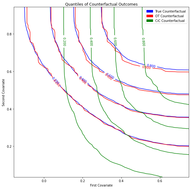
Figure 7: Quantiles of the empirical CDF over a uniform mesh with $10,000$ points.

4.2 Revisiting the Card & Krueger dataset

On April 1, 1992, New Jersey raised its minimum wage from the Federal level of $\$4.25$ per hour to $\$5.05$ per hour. Card and Krueger (1994) (CK henceforth) investigated the effect this increase had on employment in fast food restaurants with a case-control experimental design, taking the bordering region of eastern Pennsylvania, where the minimum wage remained at $\$4.25$, as a control group. The original study employs the standard DiD estimator to conclude that the higher minimum wage led to increased employment in New Jersey restaurants. This result spawned much debate within the economics community about the effect of minimum wage policies on employment (e.g. Neumark and Wascher 2000, Dube et al. 2010, Meer and West 2016, Neumark et al. 2014 and references therein). We obtained a copy of the full dataset from David Card’s public website.

The treatment effect of interest in CK and many subsequent reevaluations is the change in full-time equivalent employees (FTE), which is defined via ${\text{FTE}=\text{FT}+.5\text{PT}}$, where FT (PT) is the number of full-time (part-time) employees (Neumark and Wascher, 2000; Lu and Rosenbaum, 2004). We use the proposed multivariate extension of the changes-in-changes estimator to estimate a bivariate treatment effect in terms of full- and part-time employees, hence fully dissecting the causal effect of raising the minimum wage on these subgroups.

The original CK study finds a positive average treatment effect of $2.76$ FTE jobs added in the treatment group compared to the control group, a result reproduced by Neumark and Wascher (2000) using different methodology. Neumark and Wascher (2000) also compute an average treatment effect in full- and part-time jobs with separate regressions and find treatment effects of $3.16$ gained full-time jobs and $0.60$ lost part-time jobs. These classical contributions only focus on aggregate outcomes over all restaurants, irrespective of the size of the respective restaurant. An exception is Ropponen (2011) who reanalyzes the data with the CiC estimator, taking into account the heterogeneity in the size of the fast-food restaurants. He finds the average treatment effect bounded in $[0.90,1.70]$. Ropponen also notes in New Jersey that large restaurants pre-intervention (measured in FTE employees) have a negative treatment effect while small restaurants pre-intervention have a positive treatment effect. Our analysis recovers this trend for both FT and PT employees in New Jersey. As we also generate counterfactual controls, we find an opposite trend for Pennsylvania restaurants. This opposite trend is intriguing and worth exploring further as it does not seem to be explained by substitution effects of employees moving across the state line to find jobs.

	OT	CiC	DiD
ATE FT	$3.07$	$2.61$	$3.45$
ATE PT	$-1.79$	$-1.52$	$-1.00$

Table 2: Estimated average treatment effect on full- and part-time employment by method.

The proposed multivariate extension of the changes-in-changes estimator allows us to jointly estimate the effects on full- and part-time employment while accounting for the heterogeneity in restaurant size. For the results in this section, restaurants are represented in $\mathbb{R}^{2}$ by our outcomes of interest, the number of full- and part-time employees. In the appendix we provide an additional experiment with restaurants represented in higher dimension including additional measurements about wages, prices, and operations. We discard $19$ units with missing outcomes, leaving $76$ control and $315$ treatment restaurants. The transport plans for both groups are solved with a linear program, and we applly nearest neighbor matching between treatment and control pre-intervention samples to calculate counterfactual outcomes.

Our optimal transport analysis suggests that fast food restaurants responded to an increased minimum wage by substituting full-time employees for part-time ones with a net gain of full-time equivalent employees. Our results seem to indicate that the negative effect on part-time employees is more pronounced than previously estimated. The quantile plot in Figure 8 suggests this effect applies throughout the distribution of restaurants, not just the mean: fixing the number of full-time employees, counterfactual quantiles tend to have more part-time employees than treated quantiles at the same level; likewise fixing the number of part-time employees, treated quantiles tend to have more full-time employees. In their original paper CK suggest that restaurants may respond to higher labor costs with more full-time employees because they tend to be older, more skilled, and more productive, thus a better investment of capital. Furthermore, the univariate methods may underestimate the number of part-time employees lost, a conclusion supported by the higher dimensional analysis in Table 5 from the appendix.

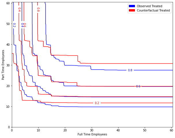
Figure 8: Post-intervention quantile curves for observed treated units and their counterfactuals.

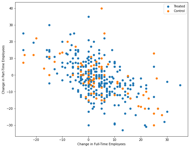
Figure 9: Distribution of unit-level treatment effect estimates, demonstrating a negative correlation between change in full-time and part-time employeest.

5 Discussion

We have introduced a general method based on optimal transport theory for causal inference in classical treatment and control study designs. It combines two desirable properties: it is designed for high dimensional settings while at the same time capturing the heterogeneity in treatment response of individuals. In particular, it generalizes both the classical difference-in-differences estimator, which is applicable in high dimension but only captures average effects, and the changes-in-changes estimator (Athey and Imbens, 2006), which allows for general treatment heterogeneity but is only applicable in univariate settings. It also implies a natural and interpretable generalization of the standard “parallel trends” assumption of difference-in-difference estimators (Abadie, 2005) in terms of co-monotonicity of the causal production functions.

Showcasing the utility of the proposed method, we revisit the classical Card & Krueger dataset by decomposing the treatment effects for full-and part-time employees. We find that fast-food restaurants responded to an increased minimum wage by substituting full-time employees for part-time employees, even when accounting for restaurant size. This provides a novel insight by dissecting the relationship between full- and part-time employees while accounting for the heterogeneity in restaurant size. More generally, since our proposed method is able to consider multivariate outcomes, it can help uncover interesting causal effects and nonlinear relations in a wide array of applications.

Appendix A Omitted proofs and experiment details

A.1 Omitted proofs from the main text

Proof of Theorem 3

Proof A.1.

Recall first that the co-monotonicity assumption (A.3) reads as

$$\langle h_{0}(x)-h_{0}(y),h_{1}(x)-h_{1}(y)\rangle\geq 0\qquad\forall\,x,y\in\mathbb{R}^{d}\,.$$

Define $x_{0}=h_{0}(x),y_{0}=h_{0}(y)$ so that

$$\langle x_{0}-y_{0},h_{1}\circ h_{0}^{-1}(x_{0})-h_{1}\circ h_{0}^{-1}(y_{0})\rangle\geq 0$$

for all $x_{0},y_{0}$ in the image of $h_{0}$. In particular, this implies that the function $\mathsf{d}=h_{1}\circ h_{0}^{-1}$ is monotone in the sense of (4). Since the function maps a convex set $K_{0}$ to a finite set $F_{1}$, it follows from Theorem 2 that $\mathsf{d}$ is, in fact, cyclically monotone. By Rockafellar (1997, Theorem 24.8), this is equivalent to $\mathsf{d}$ being the gradient of a convex function and, hence the unique Brenier map from $\mu_{0}$ to $\mu_{1}$. This completes the first part of the theorem.

The second part of the theorem follows exactly the same arguments with $h_{1}^{\star}$ replacing $h_{1}$.

Proof of Co-monotone Production Functions in 4.1

Proof A.2.

Recall we defined the following production functions in our synthetic data experiment:

$$h_{0}(u)=\begin{bmatrix}1&\alpha\\ \alpha&1\end{bmatrix}u\qquad\text{and}\qquad h_{1}(u)=\begin{bmatrix}1&-\alpha\\ -\alpha&1\end{bmatrix}u.$$

In our simulations, the $\alpha$ parameter of the production functions is fixed at $0.5$. This choice makes $h_{0}$ and $h_{1}$ co-monotone, because for $\alpha<1$

$$\begin{bmatrix}1&\alpha\\ \alpha&1\end{bmatrix}\cdot\begin{bmatrix}1&-\alpha\\ -\alpha&1\end{bmatrix}=\begin{bmatrix}1-\alpha^{2}&0\\ 0&1-\alpha^{2}\end{bmatrix}\geq 0.$$

Note, however, that $h_{0}$ and $h_{1}$ are not element-wise monotone as required by the CiC estimator. In fact, the first marginal function $h_{0}^{(1)}$ and $h_{1}^{(1)}$satisfy

$$\langle h_{0}^{(1)}(u)-h_{0}^{(1)}(v),h_{1}^{(1)}(u)-h_{1}^{(1)}(v)\rangle=\begin{bmatrix}1&\alpha\end{bmatrix}(u-v)\cdot\begin{bmatrix}1&-\alpha\end{bmatrix}(u-v).$$

Hence by setting $(u-v)\equiv\begin{bmatrix}0&z\end{bmatrix}^{\top}$ for some $z\neq 0$ it holds that

$$\langle h_{0}^{(1)}(u)-h_{0}^{(1)}(v),h_{1}^{(1)}(u)-h_{1}^{(1)}(v)\rangle=(\alpha z)\cdot(-\alpha z)=-\alpha^{2}z^{2}<0.$$

A.2 Implementation Details

In this section we provide details about the implementation of our numerical experiments from Section 4. In our experiments, we obtain finite draws from the continuous distributions $\nu$ and $\nu^{\star}$ to apply production functions and generate $\mu_{0}$ and $\mu_{0}^{\star}$ and post-intervention outcomes $\mu_{1}$ and $\mu^{\dagger}_{1}$.

Recent results prove consistency (Panaretos and Zemel 2020, de Lara et al. 2021) and rates of convergence under smoothness assumptions (Hütter and Rigollet 2021, Gunsilius 2021, Vacher et al. 2021) of optimal transport maps computed from empirical sample data. Because of these advances, we claim the transport maps calculated on large, but finite, simulation datasets estimate the true infinite-population maps well.

To compute optimal transport maps, we use a linear programming method ot.lp.emd from the Python package Python Optimal Transport (Flamary et al., 2021). These maps are then extrapolated into optimal transport plans with Euclidean nearest neighbor matching. In our simulations the control and treatment groups pre-intervention have almost complete overlap of sampled support, justifying this technique. To be concrete, counterfactual treatment outcomes are generated by matching each treatment unit pre-intervention to the nearest control and pushing forward along the transport map between observed control distributions.

All numerical experiments are written and run in Python 3.

A.3 Additional Card & Krueger Experiment

For our reanalysis of the Card & Krueger data on the minimum wage and fast food employment, we use the original dataset provided by David Card on his website. It contains survey information, collected via telephone, for $410$ fast food restaurants across $4$ fast-food chains. Of these, $79$ are in the control region of northeastern Pennsylvania and $331$ are in New Jersey. In addition to the two employment outcomes of interest, a number of other observations about a restaurant’s wages, prices, and operations were collected. Our optimal transport methodology allows us to estimate treatment effects with restaurants more richly represented as vectors in $\mathbb{R}^{10}$. We present this experiment for illustrative purposes.

Covariate Name	Description
EMPFT	Number of full-time employees
EMPPT	Number of part-time employees
PCTAFF	Percent of employees affected by new minimum wage
NMGRS	Number of managers
INCTIME	Months until usual first raise
PENTREE	Price of an entrée with tax
PSODA	Price of a soda with tax
NREGS	Number of cash registers in the restaurant
OPEN	Hour of opening
HRSOPEN	Number of hours open per day

Table 3: Outcomes and covariates included in our analysis.

We select a representative subset of $10$ numerical covariates, listed in Table 3, and remove any restaurant with a missing entry for any of these covariates. This leaves a final sample of $52$ controls and $200$ treated. The full dataset has $15$ numerical covariates but including all $15$ leads to a small sample size due to missing data. The covariates we do not include add little additional information, such as the price of fries (we include the price of entrées and sodas), have high rates of missingness, or have a different distribution in the subsample with complete data than the entire survey population. Unlike the outcome-only analysis presented in Section 4.2, the included covariates have different scales. Thus, we standardize each to zero mean and unit standard deviation. The dataset also includes categorical data such as the fast-food chain, which we do not include because the distance between restaurants would depend on how these are encoded.

We observed moderate sensitivity of estimate magnitude when perturbing the covariate set, although the sign of our estimators did not change. Therefore, we present aggregate results over subsets of covariates and units in this experiment. We believe the difficulty of estimating a $10$ dimensional object with only $250$ observations leads to this sensitivity and use more robust experiment design to smooth out the randomness. Table 4 shows that including additional covariates does not change the sign of our estimated treatment effects and estimates both full-time and part-time employment changes with smaller magnitude than bivariate optimal transport. Like the results in Section 4.2, this analysis suggests the minimum wage increase led the average fast food restaurant to hire more FTE employees and that univariate methods may underestimate the part-time treatment effect.

	Mean OT w/ Covariates	OT	CiC	DiD
ATE FT	$1.54$	$3.12$	$3.08$	$4.03$
ATE PT	$-1.66$	$-2.12$	$-0.84$	$-0.97$

Table 4: Estimated treatment effects with and without covariates by method in the covariate-complete subpopulation.

To temper sensitivity to certain covariates, we calculate the treatment effects for all subsets of covariates in $\mathbb{R}^{8}$, $\mathbb{R}^{9}$, or $\mathbb{R}^{10}$. The positive results of this experiment are included in Table 5. The sign of our two estimates never change in this experiment. To show our results are not biased by any particular units, we rerun our experiment $10000$ times with $20\%$ of our treatment and control units randomly dropped but all covariates included. Further reinforcing the estimates’ consistency in sign, the effect for part-time workers becomes positive above the $96^{\text{th}}$ quantile and the effect for full-time workers becomes negative below the $1^{\text{st}}$ quantile. Both checks suggest the full-time treatment effect given by optimal transport with covariates is smaller than univariate estimates, while classical methods may underestimate the decrease in part-time workers. In future work with more tests for covariate selection and further sensitivity analysis, we hope stronger claims about the estimates’ magnitude can be made.

	TE FT	TE PT
Mean	$1.54$	$-1.66$
st. dev.	$0.84$	$0.99$
Min	$0.34$	$-3.14$
Max	$2.46$	$-0.62$

(a) Removed covariates

	TE FT	TE PT
Mean	$1.66$	$-1.70$
st. dev.	$0.84$	$0.99$
Min	-$1.30$	$-5.24$
Max	$4.60$	$1.70$

(b) Removed units

Table 5: Summary statistics of our robustness checks for the Card & Krueger ATE.

References

- Abadie (2005) Alberto Abadie. Semiparametric difference-in-differences estimators. Review of Economic Studies, 72(1):1–19, 2005.
- Angrist and Pischke (2008) Joshua D Angrist and Jörn-Steffen Pischke. Mostly harmless econometrics: An empiricist’s companion. Princeton university press, 2008.
- Athey and Imbens (2006) Susan Athey and Guido W Imbens. Identification and inference in nonlinear difference-in-differences models. Econometrica, 74(2):431–497, 2006.
- Bates et al. (2020) Stephen Bates, Matteo Sesia, Chiara Sabatti, and Emmanuel Candès. Causal inference in genetic trio studies. Proceedings of the National Academy of Sciences, 117(39):24117–24126, 2020.
- Belyaeva et al. (2021) Anastasiya Belyaeva, Louis Cammarata, Adityanarayanan Radhakrishnan, Chandler Squires, Karren Dai Yang, GV Shivashankar, and Caroline Uhler. Causal network models of SARS-CoV-2 expression and aging to identify candidates for drug repurposing. Nature communications, 12(1):1–13, 2021.
- Bonhomme and Sauder (2011) Stéphane Bonhomme and Ulrich Sauder. Recovering distributions in difference-in-differences models: A comparison of selective and comprehensive schooling. Review of Economics and Statistics, 93(2):479–494, 2011.
- Brenier (1991) Yann Brenier. Polar factorization and monotone rearrangement of vector-valued functions. Communications on Pure and Applied Mathematics, 44(4):375–417, 1991.
- Caffarelli (2000) Luis A. Caffarelli. Monotonicity properties of optimal transportation and the FKG and related inequalities. Comm. Math. Phys., 214(3):547–563, 2000.
- Callaway and Li (2019) Brantly Callaway and Tong Li. Quantile treatment effects in difference in differences models with panel data. Quantitative Economics, 10(4):1579–1618, 2019.
- Card and Krueger (1994) David Card and Alan B Krueger. Minimum wages and employment: A case study of the fast-food industry in New Jersey and Pennsylvania. American Economic Review, 84(4):772–793, 1994.
- Chernozhukov and Hansen (2005) Victor Chernozhukov and Christian Hansen. An IV model of quantile treatment effects. Econometrica, 73(1):245–261, 2005.
- Chernozhukov et al. (2021) Victor Chernozhukov, Alfred Galichon, Marc Henry, and Brendan Pass. Identification of hedonic equilibrium and nonseparable simultaneous equations. Journal of Political Economy, 129(3):842–870, 2021.
- de Lara et al. (2021) Lucas de Lara, Alberto González-Sanz, and Jean-Michel Loubes. A consistent extension of discrete optimal transport maps for machine learning applications. arXiv preprint 2102.08644, 2021.
- Doksum (1974) Kjell Doksum. Empirical probability plots and statistical inference for nonlinear models in the two-sample case. The Annals of Statistics, pages 267–277, 1974.
- Drysdale and Hendricks (2018) Krystal M. Drysdale and Nathan P. Hendricks. Adaptation to an irrigation water restriction imposed through local governance. Journal of Environmental Economics and Management, 91:150–165, 2018.
- Dube et al. (2010) Arindrajit Dube, T William Lester, and Michael Reich. Minimum wage effects across state borders: Estimates using contiguous counties. Review of Economics and Statistics, 92(4):945–964, 2010.
- Firpo (2007) Sergio Firpo. Efficient semiparametric estimation of quantile treatment effects. Econometrica, 75(1):259–276, 2007.
- Flamary et al. (2021) Rémi Flamary, Nicolas Courty, Alexandre Gramfort, Mokhtar Z. Alaya, Aurélie Boisbunon, Stanislas Chambon, Laetitia Chapel, Adrien Corenflos, Kilian Fatras, Nemo Fournier, Léo Gautheron, Nathalie T.H. Gayraud, Hicham Janati, Alain Rakotomamonjy, Ievgen Redko, Antoine Rolet, Antony Schutz, Vivien Seguy, Danica J. Sutherland, Romain Tavenard, Alexander Tong, and Titouan Vayer. POT: Python optimal transport. Journal of Machine Learning Research, 22(78):1–8, 2021.
- Forrow et al. (2019) Aden Forrow, Jan-Christian Hütter, Mor Nitzan, Philippe Rigollet, Geoffrey Schiebinger, and Jonathan Weed. Statistical optimal transport via factored couplings. In The 22nd International Conference on Artificial Intelligence and Statistics, pages 2454–2465. PMLR, 2019.
- Goodman-Bacon and Marcus (2020) Andrew Goodman-Bacon and Jan Marcus. Using difference-in-differences to identify causal effects of COVID-19 policies. DIW Berlin Discussion Paper No. 1870, 2020.
- Gunsilius (2021) Florian F Gunsilius. On the convergence rate of potentials of Brenier maps. Econometric Theory, 2021. To appear.
- Heckman (1990) James Heckman. Varieties of selection bias. The American Economic Review, 80(2):313–318, 1990.
- Ho and Rubin (2011) Daniel E Ho and Donald B Rubin. Credible causal inference for empirical legal studies. Annual Review of Law and Social Science, 7:17–40, 2011.
- Holland (1986) Paul W Holland. Statistics and causal inference. Journal of the American Statistical Association, 81(396):945–960, 1986.
- Hütter and Rigollet (2021) Jan-Christian Hütter and Philippe Rigollet. Minimax estimation of smooth optimal transport maps. The Annals of Statistics, 49(2):1166 – 1194, 2021.
- Imbens and Rubin (2015) Guido W Imbens and Donald B Rubin. Causal inference in statistics, social, and biomedical sciences. Cambridge University Press, 2015.
- Kushnir and Lokutsievskiy (2021) Alexey I. Kushnir and Lev V. Lokutsievskiy. When is a monotone function cyclically monotone? Theoretical Economics, 2021. To appear.
- Lechner (2011) Michael Lechner. The estimation of causal effects by difference-in-difference methods. Foundations and Trends® in Econometrics, 4(3):165–224, 2011.
- Lehmann (1974) Erich Leo Lehmann. Nonparametrics: statistical methods based on ranks. Holden-day, 1974.
- Lu and Rosenbaum (2004) Bo Lu and Paul R Rosenbaum. Optimal pair matching with two control groups. Journal of Computational and Graphical Statistics, 13(2):422–434, 2004.
- Meer and West (2016) Jonathan Meer and Jeremy West. Effects of the minimum wage on employment dynamics. Journal of Human Resources, 51(2):500–522, 2016.
- Meinshausen et al. (2016) Nicolai Meinshausen, Alain Hauser, Joris M Mooij, Jonas Peters, Philip Versteeg, and Peter Bühlmann. Methods for causal inference from gene perturbation experiments and validation. Proceedings of the National Academy of Sciences, 113(27):7361–7368, 2016.
- Morgan and Winship (2014) Stephen L. Morgan and Christopher Winship. Counterfactuals and Causal Inference: Methods and Principles for Social Research. Analytical Methods for Social Research. Cambridge University Press, 2 edition, 2014.
- Neumark and Wascher (2000) David Neumark and William Wascher. Minimum wages and employment: A case study of the fast-food industry in New jersey and Pennsylvania: Comment. American Economic Review, 90(5):1362–1396, 2000.
- Neumark et al. (2014) David Neumark, JM Ian Salas, and William Wascher. Revisiting the minimum wage—employment debate: Throwing out the baby with the bathwater? ILR Review, 67(3_suppl):608–648, 2014.
- Neyman (1923) J. Neyman. Sur les applications de la théorie des probabilités aux expériences agricoles : Essai des principes. Masters thesis. Excerpts reprinted in English, Statistical Science, Vol. 5, pp. 463–472. (D. M. Dabrowska, and T. P. Speed, Translators.), 1923.
- Panaretos and Zemel (2020) Victor M Panaretos and Yoav Zemel. An invitation to statistics in Wasserstein space. Springer Nature, 2020.
- Peyré and Cuturi (2019) Gabriel Peyré and Marco Cuturi. Computational optimal transport. Foundations and Trends® in Machine Learning, 11(5-6):355–607, 2019.
- Rigollet and Weed (2019) Philippe Rigollet and Jonathan Weed. Uncoupled isotonic regression via minimum Wasserstein deconvolution. Information and Inference: A Journal of the IMA, 04 2019.
- Rockafellar (1997) Ralph Tyrell Rockafellar. Convex analysis. Princeton university press, 1997.
- Ropponen (2011) Olli Ropponen. Reconciling the evidence of Card and Krueger (1994) and Neumark and Wascher (2000). Journal of Applied Econometrics, 26(6):1051–1057, 2011.
- Roth and Sant’Anna (2020) Jonathan Roth and Pedro HC Sant’Anna. When is parallel trends sensitive to functional form? arXiv preprint 2010.04814, 2020.
- Rothman and Greenland (2005) Kenneth J Rothman and Sander Greenland. Causation and causal inference in epidemiology. American Journal of Public Health, 95(S1):S144–S150, 2005.
- Rubin (1974) Donald B Rubin. Estimating causal effects of treatments in randomized and nonrandomized studies. Journal of Educational Psychology, 66(5):688, 1974.
- Rubin (1978) Donald B. Rubin. Bayesian inference for causal effects: The role of randomization. The Annals of Statistics, 6(1):34–58, 1978.
- Ryan et al. (2019) Andrew M Ryan, Evangelos Kontopantelis, Ariel Linden, and James F Burgess Jr. Now trending: Coping with non-parallel trends in difference-in-differences analysis. Statistical Methods in Medical Research, 28(12):3697–3711, 2019.
- Saks and Yu (2005) Michael Saks and Lan Yu. Weak monotonicity suffices for truthfulness on convex domains. In Proceedings of the 6th ACM conference on Electronic commerce, pages 286–293, 2005.
- Shi et al. (2018) Xiaoxia Shi, Matthew Shum, and Wei Song. Estimating semi-parametric panel multinomial choice models using cyclic monotonicity. Econometrica, 86(2):737–761, 2018.
- Squires et al. (2020) Chandler Squires, Dennis Shen, Anish Agarwal, Devavrat Shah, and Caroline Uhler. Causal imputation via synthetic interventions. arXiv preprint 2011.03127, 2020.
- Vacher et al. (2021) Adrien Vacher, Boris Muzellec, Alessandro Rudi, Francis Bach, and Francois-Xavier Vialard. A dimension-free computational upper-bound for smooth optimal transport estimation. In COLT 21, 2021.
- Wing et al. (2018) Coady Wing, Kosali Simon, and Ricardo A Bello-Gomez. Designing difference in difference studies: best practices for public health policy research. Annual Review of Public Health, 39, 2018.