Logit Attenuating Weight Normalization

Abstract

Over-parameterized deep networks trained using gradient-based optimizers are a popular choice for solving classification and ranking problems. Without appropriately tuned $\ell_{2}$ regularization or weight decay, such networks have the tendency to make output scores (logits) and network weights large, causing training loss to become too small and the network to lose its adaptivity (ability to move around) in the parameter space. Although regularization is typically understood from an overfitting perspective, we highlight its role in making the network more adaptive and enabling it to escape more easily from weights that generalize poorly. To provide such a capability, we propose a method called Logit Attenuating Weight Normalization (LAWN), that can be stacked onto any gradient-based optimizer. LAWN controls the logits by constraining the weight norms of layers in the final homogeneous sub-network. Empirically, we show that the resulting LAWN variant of the optimizer makes a deep network more adaptive to finding minimas with superior generalization performance on large scale image classification and recommender systems. While LAWN is particularly impressive in improving Adam, it greatly improves all optimizers when used with large batch sizes.

1 Introduction

The advent of large scale deep models with tens of millions to billions of parameters has resulted in three trends in the community: (1) State-of-the-art performance on over-parameterized networks for problems like image classification, language modeling, machine translation, text classification and recommender systems. (2) Development of optimizers like Stochastic Gradient Descent (SGD) with heavy-ball momentum (qian1999momentum, ), Adam (kingma2017adam, ), AdamW (loshchilov2019decoupled, ), LAMB (you2020large, ) and their extensions with $\ell_{2}$ regularization and weight decay to improve generalization performance. (3) Increased emphasis on theory to understand the optimizer landscape, especially how to tune different hyperparameters well to escape poor minima for both large and small batch sizes. In this work, inspired by all three trends, we propose a new training method, explain why it works, and show improved performance over popular optimizers across a wide range of batch sizes for classification and ranking tasks.

Complex deep networks can easily learn to classify a large fraction of examples correctly as training progresses. These networks have two characteristics: (a) they have one or more contiguous homogeneous layers at the end forming the final homogeneous sub-network, and, (b) they are trained with exponential-type loss functions like logistic loss and cross entropy that asymptotically attain their least value of zero when the network score goes to infinity. Let us collectively refer to this network score as logit. After the network has learned to correctly classify a large fraction of training examples, the weights of the end homogeneous layers and the logits grow to make the training loss (and hence its gradient) very small. This, seen in optimizers like SGD (Bottou2010, ) and Adam  (kingma2017adam, ) when used with no (or mild) $\ell_{2}$ regularization or weight decay, leads to loss flattening (Details in Appendix B). This further leads to loss of adaptivity of the network (szegedy2016rethinking, ), causing training to stall in regions of sub-optimal generalization.

Figure 1 shows the generalization performance (Test HR@10) of Adam (green dotted line) applied to a fully homogeneous network on a classification task. After $115$ epochs, Margin p50 (median margin over the training examples; blue dotted line) becomes large and the training gets stuck in the basin of a sub-optimally generalizing minimum. The minimum is also overfitting due to the tussle between good and noisy examples.

Figure 1: Adam with (continuous lines) and without (dotted lines) logit attenuation on MovieLens classification. Adam: after $115$ epochs (vertical dotted black line), loss flattening sets in, Test HR@10 is sub-optimal, with overfitting. Adam with logits attenuation: The introduction of $\alpha$ factor after the $115$th epoch reduces Margin p50 but keeps Test HR@10 the same. Though Test HR@10 then drops initially, with further constrained weight training Adam with logit attenuation eventually achieves a higher Test HR@10 than vanilla Adam.

Optimizer	Batch Size
	256	16k
SGD	76.00 (0.04)	74.48 (0.06)
SGD-L	76.12 (0.01)	75.56 (0.02)
Adam	71.16 (0.05)	70.60 (0.02)
Adam-L	76.18 (0.03)	76.07 (0.08)
LAMB+	74.30 (0.01)	73.43 (0.03)
LAMB-L	76.48 (0.05)	75.93 (0.02)

Table 1: ImageNet validation accuracy. Comparison of LAWN variants (*-L) of different optimizers with their base variants on the ImageNet validation set. LAWN enables Adam to work on image classification tasks with very little drop in performance at large batch sizes. Current optimizers have a much steeper drop-off in performance as batch size increases. Standard error is mentioned in parentheses.

Consider that training has reached a point where logits are becoming large. There are two ways of attenuating the logit values: (a) multiply the logits by a factor, $0<\alpha<1$ and use this factor for the rest of the training; (b) constrain the norms of layer weights for the rest of the training. To provide a rough demonstration of the value of these methods, we return to the experiment of Figure 1 and, after epoch $115$, we shrink the logits to one-fifth, and then continue training while keeping the weight norms of each layer fixed. This leads to superior generalization with no overfitting toward the end of training. Method (a) alone is not sufficient since further training will increase the logits again to reduce the training loss. Method (b) is more effective; also, in this case we could have worked with smaller logits by switching to constrained training very early.

Our method, Logit Attenuating Weight Normalization (LAWN) can be used with any gradient-based base optimizer. LAWN begins with normal, unconstrained training in the initial phase and then fixes the weight norms of the layers for the rest of the training. The training on the constrained norm surfaces is done by employing projected gradients instead of regular gradients.

Although, adaptive methods like Adam have known to struggle with convolutional neural networks, the LAWN variant of Adam achieves very impressive performance across multiple network architectures and tasks. At large batch sizes, most optimizers get caught in sub-optimal regions due to lowered stochasticity which is worsened by increased logits. LAWN’s attenuation of the logits helps avoid this worsening. Due to this, the LAWN variants of SGD, Adam and LAMB work significantly better than their base versions at large batch sizes. Table 1, which compares the generalization performance of SGD, Adam and LAMB against their LAWN variants on the popular Imagenet dataset, powerfully showcases the two observations on LAWN mentioned above.

In the following sections, we motivate (§2) and develop LAWN (§3) as a new training method. We then proceed to show (§4) that LAWN effectively improves adaptivity of networks and leads to much better generalization than known methods, e.g. $\ell_{2}$ regularization and weight decay using a wide variety of networks for image classification (CIFAR, ImageNet) and recommender systems (MovieLens, Pinterest).

2 The Need for LAWN

In this section we motivate LAWN by describing the problem settings in which normal training struggles and in which LAWN could improve generalization performance. We define these problem settings in §2.1, then describe what we mean by loss of adaptivity in §2.2. We review the strengths and weaknesses of existing methods for avoiding loss of adaptivity in §2.3. With this context, we elaborate on the LAWN method in §3.

Notations. For the rest of the paper we will use multi-class setting as the running example. The following notations will be used: $n$ is the number of weight variables; $m$ is the number of training examples; $i$ is the index used to denote the index of a training example; $y_{i}$ is the target class of the $i$-th training example; $k$ is the index used to denote a class; $nc$ is the number of classes; $w$ is the weight vector of the deep net; $p_{k}(w)$ is the class $k$ probability assigned by the deep net with weight vector $w$. For an optimizer, $\eta$ denotes the learning rate and $B$ is the batch size.

2.1 When does LAWN work?

Let us describe the problem settings in which we expect generalization improvement using LAWN.

Problem type. We are mainly interested in classification and ranking problems which form a score for the target. In binary classification this score is the logit score of the target class; in a multiclass problem, this score is the difference between the target class score and the maximum score over the remaining classes. For ease of presentation we will simply refer to such scores as logit. We consider a loss function that attains its least value (usually zero) asymptotically as logit goes to infinity. The logistic loss for binary classification and the cross entropy loss based on softmax for multi-class classification are important cases. Problems like regression that use a loss function such as the squared loss (which attains its minimum at a finite value) may not have much benefit using LAWN. In a multi-task setting, when the total loss is an additive mix of several individual task losses, LAWN can be useful even if just one of them is suited for LAWN.

Homogeneity. A network layer is said to be homogeneous if multiplying either all weights or all incoming signals of the layer by a constant $\alpha$ leads to the output of the layer being multiplied by $\alpha$. The presence of bias weights in a layer causes a violation of homogeneity since the input multiplied by them is always $1$, i.e., $W(\alpha x)+b\not=\alpha(Wx+b)$. Since the number of bias weights in any layer is small, we will ignore this as a minor issue and take a layer (which is otherwise homogeneous) to be homogeneous for all theoretical reasoning; also, see Lyu and Li (lyu2020gradient, ) for a discussion of this matter. A layer of linear or relu units is homogeneous. When classification and ranking problems are used, the final layer of the network is usually linear (it generates the class scores) and hence homogeneous. Homogeneity in the end layer(s) is the reason for logit to become large and hence it plays a key role in the utility of LAWN. A maximal contiguous set of homogeneous layers of a network will be referred to as a homogeneous subnet.

The final layer that forms the class scores and all preceding contiguous homogenous layers is called the final homogeneous subnet (fhsn). In the case of a batch normalization (BN) layer, we can break the layer into two sublayers: the first sublayer does normalization (non-homogeneous) over a batch of examples, and the following second sublayer applies scaling (homogeneous) and shift (which is akin to bias weights). Thus, when BN is encountered, the second sublayer is treated as homogeneous and, if it is immediately followed by a homogeneous activation function, then it gets included as a part of the homogeneous subnet that follows it. Similar ideas hold for other normalizations such as layer normalization. We will refer to the weights in fhsn as $w_{fhsn}$. Figure 2 gives an example to illustrate these definitions.

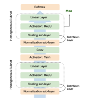
Figure 2: Homogeneous layers are shown in green, with each homogeneous subnet marked in dotted lines. fhsn is the final homogeneous subnet.

When fhsn contains all the layers of the network, we call it a fully homogeneous network. Fully homogeneous networks are popularly used in recommender systems (he2017neural, ; zhang2019deeprecsyscsur, ).

Network Complexity. This refers to the complexity of the network in relation to the number of training examples. Most deep networks used in applications are over-parametrized. Roughly, we will take over-parametrized to mean that the network is so powerful that training easily locates a $w$ that classifies all examples correctly, i.e., the target class has the highest score among all classes. Given the presence of fhsn which can lead to large logit scores, this would also mean that, by making $w_{fhsn}$ go to $\infty$ we can make the training loss go to zero.

For LAWN to work usefully, we do not require over-parametrization per se, but a network which is very flexible and training easily pushes the loss of most training examples very small. A small set of examples can remain misclassified; for example, this often happens when data augmentation is used. Below, in §2.2 we will explain how this situation of most examples attaining very small loss values creates an issue.

Generalization Metrics. Our focus is on improving metrics that are based on score ordering as opposed to the actual values of scores. More precisely, we are interested in test set metrics such as classification error, AUC, NDCG etc. as opposed to logistic loss, cross entropy loss, probability calibration error etc. Deep networks are known to be poor with respect to the latter metrics (GuoPSW17, ) but which can be improved in the post-training stage; the adaptation of LAWN to improving such metrics will be taken up in a follow-up work.

2.2 Issue of loss of adaptivity

Consider the problem setting defined in §2.1 and the minimization of the normally used unregularized training loss, $L(w)=-\frac{1}{m}\sum_{i=1}^{m}\log p_{y_{i}}(w)$. With the network being sufficiently powerful, training causes the losses of a large fraction of the training examples to become very small. During training, this happens due to $w_{fhsn}$ becoming large, the logit becoming large, and $p_{y_{i}}\rightarrow 1$ for those examples. Due to these, each of the following become very small: the gradient of most example-wise loss terms; $\Sigma$, the covariance of the noise associated with minibatch gradient; and, $H$, the Hessian of the training loss. We will refer to this collective happening as loss flattening.

It has been established via theoretical and empirical arguments that the powerful generalization ability of a deep net comes from its ability to escape regions of attraction of “sharper" minima with sub-optimal generalization performance and go to better solutions. Appendix F gives an idea of the escape mechanism for the SGD method using an analysis given by Wu et al (Wu_NEURIPS2018, ). It is worth recalling from there, the following rough guiding condition for SGD to escape from a poor solution: $\lambda_{\max}\{(I-\eta H)^{2}+\frac{\eta^{2}(m-B)}{B(m-1)}\Sigma\}>1$, where $\lambda_{\max}(A)$ denotes the largest eigenvalue of $A$. If training is at a sub-optimal generalization point and loss flattening occurs (which means that $H$ and $\Sigma$ become small), then the escape condition is difficult to satisfy and hence it becomes difficult for the network to escape from this solution and then train further to go to a better solution. A carefully increased learning rate schedule to cause the escape followed by the use of normal learning rates to go to a better solution can make this happen, but no such automatic sophisticated learning rate adjustment mechanism has been devised yet. We will refer to this inability of the network to escape out of a sub-optimal solution due to loss flattening as loss of adaptivity (also see §7 in  szegedy2016rethinking ).

2.3 Current methods for dealing with loss of adaptivity

Several methods have been suggested in the literature to handle the issue of loss of adaptivity. We briefly describe three key ones: label smoothing regularization (LSR) (szegedy2016rethinking, ), flooding (ishida2020we, ), and $\ell_{2}$ regularization/weight decay (loshchilov2019decoupled, ). LSR modifies $L(w)$ via making the target class less confident by fixing its probability as $(1-\epsilon_{LSR})$ and reassigning $\epsilon_{LSR}$ to the remaining classes. This makes the loss attain its minimum at finite logit values. Flooding modifies the loss as $L_{Flooding}(w)=|L\;-\;\epsilon_{Flooding}|$ so that the training process is forced to move around the hypersurface defined by $L\;-\;\epsilon_{Flooding}=0$. $\ell_{2}$ regularization is a traditional method that modifies the loss as $L_{\ell_{2}}=L(w)+\frac{\lambda}{2}\|w\|^{2}$. Weight decay, as used in the recent deep net literature decouples the term $\lambda w$ from the gradient and instead includes the additive term, $-\lambda w$ at the weight update step. Later, in §3 we will return to discuss these methods in relation to LAWN.

3 The LAWN Method

A smooth classification loss such as the one based on logistic or cross entropy functions is necessary for gradient-based training. Consider a network with weights $\bar{w}$ and corresponding fhsn weights $\bar{w}_{fhsn}$. When we extend $\bar{w}_{fhsn}$ along a radial direction, i.e., $w_{fhsn}=\alpha\bar{w}_{fhsn}$, $\alpha\in R_{+}$, while keeping the weights of the network outside fhsn unchanged, the classification error on a set of examples (e.g., the training error computed on a training set or the generalization error computed on a test set) remains unaffected whereas classification loss varies a lot with $\alpha$. In particular, if $\bar{w}$ classifies a set of examples strictly correctly, then, as $\alpha$ goes from $0$ to $\infty$, the average loss on these examples goes from $\log(nc)$ to zero asymptotically. During normal training, with weight directions having a good radial component, training loss does become very small. Earlier, in §2 we saw how, when training loss becomes very small, it causes loss flattening, which leads to a loss of adaptivity of the network. Therefore, it makes sense to suitably contain the radial movement of $w_{fhsn}$ by constraining $\|w_{fhsn}\|$. The essential spirit of LAWN is along this idea.

fhsn is a homogeneous subnet which can have more than one layer. A homogeneous subnet has many redundancies (dinh2017sharp, ). For example, we can take any one layer, multiply all weights in the layer by a constant and divide all the weights of another layer by the same constant and hence keep the input-output function of the subnet unaltered. Given this, one can choose to constrain the weights in fhsn in one of the following two ways: (a) coarsely at the full fhsn level by constraining $\|w_{fhsn}\|$; (b) finely at the layer level by constraining each $\|w_{fhsn}^{\ell}\|$ where $w_{fhsn}^{\ell}$ denotes the weights of a layer $\ell$ in fhsn. In this paper we work with constraints at the layer level since it removes more redundancies.

Consider constrained training via layer-wise weight normalization: $\|w_{fhsn}^{\ell}\|=c^{\ell}\;\forall\ell$ where the $c^{\ell}$ are kept constant. It is useful to understand how the loss contours behave as the $c^{\ell}$ go from small to big values. When the $c^{\ell}$ are large, we know that loss flattening will happen. When the $c^{\ell}$ are small, the distinction between the loss values of well classified examples and poorly classified examples diminishes and so, optimizers will find it harder to traverse the contours and go to the right place of best generalization. Given this, we take a simple and natural approach to LAWN training. We initialize the network with weights having small magnitude using a standard weight initialization method and start a given optimizer in its free (unconstrained) form. At a suitable point in that training process, with weights at some $\bar{w}$, we switch to constrained training defined by setting

$$\|w_{fhsn}^{\ell}\|=c^{\ell}\mbox{ where }c^{\ell}=\|\bar{w}_{fhsn}^{\ell}\|\;\;\forall\ell$$ (1)

The $c^{\ell}$ are fixed for the rest of the LAWN training. Constrained training corresponds to solving the optimization problem,

$$\min L(w)\mbox{ s.t. (\ref{eq:constrdef}) }$$ (2)

using a modified version of any given gradient-based optimizer.

Though the homogeneous layers outside fhsn do not contribute to the growing of the scores at the end of the network that leads to loss flattening, for better performance we have found that it is useful to constrain them too. In the case of BN, we can even constrain the weight layer that just precedes it. Thus, in LAWN, the $\ell$ in (1) can be taken to include all such weight groups in the network; we do this in our implementation and use it for all experiments reported in this paper.

The switching from free training to constrained training can be done by one of the following methods. (1) We can switch after running free training for a certain number of epochs, and tune this number as a hyperparameter using a coarse grid. (2) We can track the training accuracy (done simply and efficiently by tracking accuracy on the minibatches used) and switch to constrained training when it starts plateauing at a decent high value and still far from loss flattening. All experiments reported in this paper are done using the first method. It would be useful to try the second method in the future.

Hoffer et al hoffer2018norm gives a bounded weight normalization method which also constrains the weight norm. However, it does not combine free and constrained trainings, and it does not set up and demonstrate the use of constrained training as a powerful method for use with a general optimizer for improving the performance by overcoming loss flattening and loss of adaptivity. Also, the method, as stated in the paper, does not work well. See Table 2.

Algorithm 1 LAWN Method

1:Fix $E_{total}$ and BatchSize to suitable values.

2:Choose a set of values for $\eta_{peak}$, $E_{warmup}$ and $E_{free}$.

3:for each set of hyperparameter choices do

4:     Initialize the network weights.

5:     Start the free (unconstrained) training with linear warmup.

6:     Stop after $E_{free}$ epochs and switch to constrained training.

7:     Do constrained training with linear warmup and decay.

8:end for

LAWN Implementation. We employ a simple approach to the implementation of constrained training. Let $x$ denote a weight subvector of any group (for eg., the weights and biases of a fully connected layer constitute one group) and some generic optimizer suggests a direction $d$ for $x$ to move. To remove the radial component we modify $d\rightarrow d_{p}$ by projecting $d$ to the hyperplane with $x$ as its normal. Then we do the update $x_{new}=x+\eta d_{p}$ where $\eta$ is the learning rate. Since this step increases the norm, we complete the step with a normalization: $x_{new}\leftarrow\beta x_{new}$ where $\beta=\|x\|/\|x_{new}\|$. If an adaptive optimizer such as Adam is used, all direction-related subvectors used are changed to the corresponding projected quantities; in particular, if $g^{x}$ is the gradient subvector corresponding to $x$ then the projection of $g^{x}$ to the hyperplane with $x$ as its normal is used in all updates involving the gradient. Appendix C gives the full details of SGD-LAWN, Adam-LAWN and LAMB-LAWN.

An alternative implementation to deal with the norm constraint, $\|x\|=c$ is to define an unconstrained vector $v$ and set $x=c\;v/||v||$ and simply apply any optimizer to $v$. This is the implementation suggested in Salimans and Kingma (salimans2016weight, ); see equation (2) there. (Note, however, that Salimans and Kingma (salimans2016weight, ) keeps the radial component by including the scale parameter, $g$.) One downside with this method, which makes normalization a part of the computational graph, is that automatic differentiation through the normalizing transformation increases the computational cost Huang2021 . It is worth considering this idea in future implementations of LAWN.

Let us now write the LAWN method as a complete algorithm. The free and constrained trainings of LAWN can be done with any given optimizer. LAWN does a total of $E_{total}$ epochs; $E_{total}$ is fixed for a given dataset. After $E_{free}$ epochs of free training it switches to do constrained training for $(E_{total}-E_{free})$ epochs. Learning rate schedules are important for deep networks to attain good performance (loshchilov2019decoupled, ; liu2020variance, ; loshchilov2016sgdr, ). In free training we linearly ramp the learning rate from $0$ to $\eta_{peak}$ in $E_{free}$ epochs. In constrained training, we ramp the learning rate from $0$ to $\eta_{peak}$ in $E_{warmup}$ epochs and then linearly ramp down the learning rate from $\eta_{peak}$ to $0$ in the remaining epochs. Figure LABEL:lrsched_lawn in Appendix D shows this in detail. The LAWN algorithm is described in Algorithm 1.

Fully homogeneous nets and implicit bias. Suppose the network that we use is fully homogeneous and we have an over-parametrized training problem. For such classification problems, it has been shown that gradient descent methods (lyu2020gradient, ; Poggio2019, ; Poggio2020, ; Wang2020, ; soudry2018implicit, ) have good implicit (inductive) bias properties. Specifically, it has been shown for fully homogeneous nets that gradient-based methods asymptotically attain weight directions that maximize the normalized margin (“max margin"):

$$\max_{w}\mbox{ margin}(w)/\Pi_{\ell}\|w^{\ell}\|$$ (3)

where $\mbox{margin}(w)$ is the margin given by the network with weights $w$ on the training set. Clearly, for any $\delta^{\ell}\in R_{+}$, doing $w^{\ell}\leftarrow\delta^{\ell}w^{\ell}$ individually for each $\ell$ will not alter the value of the normalized margin. So, it is not surprising that the max margin directions can also be obtained by solving (Banburski2019, )

$$\max_{w}\mbox{ margin}(w)\mbox{. s.t. }\|w_{fhsn}^{\ell}\|=c^{\ell}\;\;\forall\ell$$ (4)

See Appendix E for a proof of this result.

Though there have been attempts at optimizing margin maximization directly (bansal2018minnorm, ), it is not worth attempting because: (a) for problems that are mildly over-parametrized, it can be very sensitive to noise and lead to poor generalization and (b) the severe non-convexity and added non-smoothness of the objective make it a very hard problem to solve.

A better approach is to blend naturally with normal training via approximating $\mbox{ margin}(w)$ by a smooth function such as $h(L_{Normal}(w))$ where $h(x)=-\log(exp(x)-1)$. Thus, (3) can be effectively approximated by

$$\max_{w}h(L(w))/\Pi_{\ell}\|w^{\ell}\|$$ (5)

Lyu and Li (lyu2020gradient, ) makes effective use of (5) in its theory of implicit bias. Since $h(x)$ decreases monotonously for positive $x$, maximizing $\mbox{ margin}(w)$ is equivalent to minimizing $L$ and this leads us directly to (2) as an approximation of (4). This is a great property of LAWN - that, its constrained optimization problem, (2), is closely connected to the implicit bias defined by (3). As the $\{c^{\ell}\}$ become large, the solutions of (2) converge in direction to the solutions of (3). Thus we can view LAWN’s constrained optimization as a way of capturing implicit bias while also avoiding loss flattening. Poggio et al (Poggio2019, ; Poggio2020, ) discuss these properties for fully homogeneous nets, but they do not point out the issue of loss flattening and loss of adaptivity and so they do not develop an effective overall training method like LAWN to overcome that issue.

LSR and Flooding do not enjoy the implicit bias property because their optima are finitely located. By themselves, they have to mainly rely on the noise associated with minibatch stochasticity for reaching points of good generalization. On the other hand, $\ell_{2}$ regularization, like LAWN, also approximates implicit bias - the former uses the weight norm in the objective function and the latter uses it in the constraints. See Appendix E for details. Having said that, (2) used by LAWN could be better because of the following reasons. (a) It does not interfere with the formation of the main classification boundary in the early phase of free training. (b) The $c^{\ell}$ values are set naturally and differently for different layers of the network and so they do not require tuning. On the other hand, the $\ell_{2}$ regularization constant, $\rho$ is a single value for all the layers and it needs to be chosen to avoid the extremes of loss flattening (which happens if $\rho$ is set too low) and too much interference with loss minimization (which happens if $\rho$ is too big). In general, $\rho$ has to be carefully tuned, say using a logarithmically spaced set of values, to get the best performance  (hanson1988comparing, ; loshchilov2019decoupled, ).

Batch Size	LSR	Flooding	WD	Hoffer	LAWN
10k	68.66	68.44	70.12	44.54	70.41
100k	67.34	67.60	69.28	45.52	70.77

Table 2: Test HR@10 (Movielens-1M) of LAWN vs. other methods for controlling loss of adaptivity. For two different batch sizes, LAWN comprehensively outperforms other methods, including Weight Decay (WD). Complete details are in Appendix D.

Though implicit bias has been proved only for fully homogeneous networks, one expects to see some form of max margin theory of implicit bias for non-homogeneous nets having fhsn  to be demonstrated in the future. fhsn is expected to play a key role in this theory. Irrespective of such a theory, the use of constrained optimization in LAWN is well-motivated for such general nets since controlling radial movements of fhsn  avoids loss flattening and loss of adaptivity.

Quick comparison with other methods. We used a recommendation systems task (MovieLens-1M classification) to compare LAWN to other methods for controlling loss of adaptivity across two different batch sizes. Table 2 shows the results. LAWN outperforms all other methods. The second best method is weight decay and hence it is used as the baseline for all remaining experiments. The weight normalization technique suggested by Hoffer et al (hoffer2018norm, ) requires a modification along the lines of LAWN in order for it do well.

LAWN and large batch sizes. For a fixed epoch budget, larger batch sizes require a smaller number of steps; combined with distributed computation this helps speed up training. However, since stochasticity of updates reduces with large batch size, the mechanism of escape from sub-optimal solutions gets affected. Thus, one usually sees a reduction in generalization performance as batch size is increased (shallue2018measuring, ). Loss flattening makes this issue worse by affecting adaptivity. LAWN, by helping overcome this issue, leads to a more graceful degradation of performance as a function of batch size. The degradation becomes far less (even zero) when the the total number of steps is allowed to decently increase with batch size.

An extended LAWN method. Suppose we keep track of a historically smoothed average logit score over an epoch, and at some point of the training find that it exceeds a threshold that is set to a value around the point where loss flattens, say 3 for logistic loss (see Appendix B for a plot of the logistic loss function). We can multiply the class scores of the network by a factor, $0<\alpha<1$ and do constrained LAWN training while also multiplying the class scores by the same fixed factor $\alpha$ for the rest of the training. Earlier, in §1, Figure 1 we demonstrated the value of this simple method for a recommender network on the Movielens datset. This can lead to an automatic way for deciding when to switch from free to constrained training. We have not used this idea in the experiments of §4.

4 Experiments

To evaluate LAWN, we compared regular and LAWN-based variants of some optimizers - SGD with momentum (qian1999momentum, ), Adam (kingma2017adam, ) and LAMB (you2020large, ). Traditionally, SGD with momentum has demonstrated strong performance for computer vision tasks  (ren2015faster, ; goyal2018accurate, ), whereas adaptive methods like Adam perform well on other domains (eg. recommender systems, text classification). To demonstrate the efficacy of LAWN across a wide variety of tasks, we conducted experiments on the CIFAR (krizhevsky2009cifar, ) and ImageNet (deng2009imagenet, ; krizhevsky2012imagenet, ) datasets for image classification, and the MovieLens (harper2015movielens, ) and Pinterest (geng2015learning, ) datasets for item recommendation. All model training code was implemented using the PyTorch library (NEURIPS2019_9015, ) and experiments were conducted on machines with NVIDIA V100 GPUs. For each experiment, we report the average test metric over 3 runs. We did not tune the Adam hyperparameters $\epsilon$, $\beta_{1}$ and $\beta_{2}$, which could have led to further improvements for Adam-LAWN.

All LAWN optimizers use a 3-phase learning rate schedule as described in §3. Base variants use a 2-phase learning rate schedule that incorporates both warmup and decay. For base variants, we tuned $E_{warmup}$, peak learning rate, and weight decay. For LAWN variants, we tuned $E_{free}$, $E_{warmup}$ and peak learning rate. Appendix D contains details about hyperparameters and their tuning.

4.1 Image Classification for CIFAR-10 and CIFAR-100

For both CIFAR-10 and CIFAR-100 (krizhevsky2009cifar, ), we used the VGG-19 CNN network (simonyan2014very, ) with 1 fully connected final layer. Our ImageNet experiments use a ResNet-based (he2015deep, ) architecture. All experiments were run with a 300 epoch budget. As seen in Table 3, LAWN variants either match or outperform the base variants across batch sizes. Adam-LAWN is particularly impressive. This is in stark contrast to earlier held beliefs that adaptive optimizers cannot match SGD’s generalization performance for image classification tasks (wilson2017marginal, ).

Effect of batch size. LAWN variants cause more graceful degradation of performance with batch size, as compared to base variants. Adam-LAWN causes almost no degradation in generalization performance even at batch size 10k (see Figures 3(a), 3(b)).

Effect of $\mathbf{E_{free}}$. We observed that switching early to LAWN mode (i.e. fixing $E_{free}$ to less than 10 epochs) usually works well for generalization. See Appendix D for details. This is consistent with our hypothesis that constrained training should kick in before loss flattening sets in.

(a) CIFAR-10

(b) CIFAR-100

(c) MovieLens-1M

(d) ImageNet

Figure 3: Adam-LAWN vs. Adam (weight decay comprehensively tuned) for a variety of datasets. Adam-LAWN causes little to no drop in generalization performance with increasing batch size.

Method	CIFAR-10			CIFAR-100
	256	4k	10k	256	4k	10k
SGD	93.99	93.48	92.99	73.49	71.68	71.07
SGD-L	93.96	93.50	93.43	73.67	72.71	71.80
Adam	93.48	92.93	92.63	70.84	68.91	68.61
Adam-L	93.91	93.74	93.84	72.99	73.12	72.97
LAMB	93.76	93.27	92.91	71.29	69.39	67.76
LAMB-L	93.67	93.22	92.92	71.25	69.68	69.16

Table 3: Test Acc. on CIFAR-10 and CIFAR-100. Standard error in the the range $[0.1,0.45]$. Details in Appendix D.

4.2 Recommendation Systems

We conducted experiments on the MovieLens-100k, MovieLens-1M and Pinterest datasets using the popular neural collaborative filtering (NCF) technique (he2017neural, ). The datasets contain ratings provided to various items by users. The model is a 3-layer MLP, the input being user and item embeddings. We use the hit ratio@10 metric (expressed as %), where we reward the model for ranking a test item in the top 10 of 100 randomly sampled items that a user has not interacted with in the past. We trained for 300 epochs for the two smallest batch sizes, and 500 epochs for the two biggest batch sizes for each dataset. Details about the datasets, pre-processing, model and evaluation can be found in Appendix D. A summary of the performance of the aforementioned optimizers on all 3 datasets can be found in Table 4. LAWN-based optimizers consistently outperform their base variants. SGD and SGD-LAWN failed to generalize well at large batch sizes and this requires further investigation.

Method	MovieLens-100k				MovieLens-1M				Pinterest
	1k	10k	100k	400k	1k	10k	100k	1M	1k	10k	100k	1M
SGD	66.33	65.58	Fail	Fail	70.91	69.31	Fail	Fail	86.62	85.57	Fail	Fail
SGD-L	66.91	66.49	Fail	Fail	70.91	70.41	Fail	Fail	86.61	85.99	Fail	Fail
Adam	66.01	66.03	63.20	63.98	69.87	70.12	69.28	68.99	87.27	85.97	85.81	85.30
Adam-L	66.81	66.91	66.24	66.14	70.80	70.41	70.77	70.66	86.85	86.61	86.04	86.06
LAMB	65.45	65.34	64.23	62.57	69.91	69.77	69.44	68.95	86.63	85.91	85.80	85.65
LAMB-L	66.56	66.54	66.52	66.14	70.86	70.86	70.68	70.34	86.83	86.25	85.99	86.07

Table 4: Test HR@10 on MovieLens and Pinterest recommendations. Standard error is in the range $[0.15,0.25]$, details in Appendix D.

Weight decay vs. LAWN. Weight decay was used and tuned for all the base optimizers since it arrests the uncontrolled growth of network weights, helping avoid of loss of adaptivity. The LAWN variants do not use weight decay but still outperform the base variants.

Effect of batch size. LAWN variants of Adam and LAMB scale to very large batch sizes (1 million for MovieLens-1M, 400k for MovieLens-100k) without any appreciable loss in accuracy. Both SGD and SGD-LAWN could only scale to batch size 10k. Adam-LAWN’s strong scalability with batch size is consistent with results obtained from the CIFAR experiments.

Effect of $\mathbf{E_{free}}$. Similar to the results of the CIFAR experiments, fixing $E_{free}$ to a small value works well for LAWN. Details are in Appendix D.

4.3 Image Classification for ImageNet

As compared to CIFAR, the ImageNet classification problem (krizhevsky2012imagenet, ) is more representative of real world classification problems. We used a variant of the popular ResNet50 (he2015deep, ) model as the classifier. We considered a small (256) and a large (16k) batch size for this experiment, and fixed training budget to be 90 epochs.

Results for batch size 256. Overall results can be found in Table 1 (see §1). SGD, used in conjunction with momentum and weight decay, has long been the optimizer of choice for image classification. We retain the tuned value for weight decay of the base SGD optimizer for the free phase of SGD-LAWN experiments. SGD-LAWN marginally outperforms SGD.

Adam is well known to perform worse than SGD for image classification tasks (wilson2017marginal, ). For our experiment, we tuned the learning rate and could only get an accuracy of 71.16%. In comparison, Adam-LAWN achieves an accuracy of more than 76%, marginally surpassing the performance of SGD-LAWN and SGD.

We found it difficult to reproduce ImageNet results using the LAMB algorithm. We made minor modifications (details in Appendix D) to the original algorithm to make it more stable, and call the resultant algorithm LAMB+. LAMB-LAWN (the LAWN version of the unmodified LAMB) comprehensively outperforms LAMB+ for batch size 256 by achieving an accuracy close to 76.5%.

Results for batch size 16k. For the large batch size of 16k, we noticed that LAWN retains strong generalization performance. Both Adam-LAWN and LAMB-LAWN achieve very high accuracy, with Adam-LAWN retaining its performance at such a large batch size by crossing the 76% test accuracy mark. This is with only additonally tuning for the LAWN variants $E_{free}$ and $E_{warmup}$.

5 Conclusion

In this paper we develop LAWN as a simple and powerful method of modifying deep net training with a base optimizer to improve weight adaptivity and lead to improved generalization. Switching from free to weight norm constrained training at an appropriate point is a key element of the method. We study the performance of the LAWN technique on a variety of tasks, optimizers and batch sizes, demonstrating its efficacy. Tremendous overall enhancement of Adam and the improvement of all base optimizers at large batch sizes using LAWN are important highlights.

Appendix A Related Work

The main paper contextually covers all related works at appropriate places. In this section we collect the key papers that are closely related to the LAWN technique and briefly discuss them.

Modern DNNs are largely “over-parameterized”, i.e. the number of model parameters outnumber the training samples. For example, modern convolutional neural networks [14, 24] have tens to hundreds of millions of parameters, and provide state-of-the-art classification performance on datasets with a few million samples [5].

The issue of loss flattening and the resulting loss of adaptivity is highlighted in [39]. Several well-known techniques are used to mitigate this issue. $\ell_{2}$ regularization is often used in conjunction with optimizers like SGD, heavy-ball momentum [33] and adaptive optimizers [22, 46, 7], among others. Recently, weight decay [27, 12], which is not the same as $\ell_{2}$ regularization for adaptive optimizers, has become popular to reign-in network weights and prevent the model from becoming overconfident on training samples. Other techniques are: (a) label smoothing regularization [39], which makes the model less confident about predictions by changing the ground-truth label distribution; and (b) flooding [19] which tries to keep the aggregate training loss to be around a specified small value.

From a theory perspective, weight norm bounding has been shown to be useful for improving generalization [29, 3]. Salimans and Kingma [35] uses weight normalization as a transformation; but, by also keeping the scale component, it ends up allowing logits to grow large. Hoffer et al [16] discusses keeping the norms of the parameters fixed, but it would require a LAWN-like method to work effectively.

A perplexing property of SGD-like optimization methods is their ability to provide strong generalization performance. It has been observed that using small batch sizes makes it easier to extract better generalization performance from networks [21]. The noise injected into the optimization procedure by stochastic mini-batch gradients and the learning rate help improve generalization performance. This makes it difficult to use large batch sizes for optimization, where the noise component of the gradient diminishes with increasing batch sizes. Large batch sizes are interesting because they can help speed up the training process by leveraging multiple machines. Poor generalization performance for large batch sizes is attributed to them stalling around "sharp" minimizers [21]. Goyal et al [9] scale ImageNet training to batch sizes of 8k without obvious loss in generalization performance, by carefully tuning parameters like learning rate and batch normalization. Other recent efforts to train large-batch models include  [17, 43, 44, 36, 45]. It is important to note that for a majority of the cited works, large batch gains do not necessarily hold across tasks or datasets.

Recent theory has shown implicit bias of optimizers to maximize the (normalized) $\ell_{2}$-margin of linear models  [38, 10] and fully homogeneous neural networks  [28, 31, 32, 40]. LAWN and $\ell_{2}$ regularization approximate this implicit bias property.

Appendix B Loss Flattening

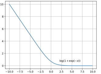
Figure 4: Logistic loss becomes small and flat if the logit crosses a threshold of 2.5 or more. Training becomes less adaptive when the losses of most examples fall in the flat zone.

Consider a binary classification problem. Figure 4 depicts the logistic loss as a function of logit. Notice that loss becomes extremely small once the logit value crosses a certain threshold (say 2.5). A small value of loss yields small gradients, making it difficult for neural network training to be adaptive. We define this as loss flattening. Multiclass classification is slightly more complex. The difference between the score of the target class and the largest score of the remaining classes plays the role of the logit and, when it becomes large enough, loss flattening occurs.

Algorithm 2 ResetState($m$, $v$)

1:Input: First moment $m$ and second moment $v$

2:Output: Updated $m$ and $v$

3:$m$ = 0

4:$v$ = 0

Algorithm 3 Project($g^{\ell}$, $w^{\ell}$, $c^{\ell}$, $k$, $t$)

1:Input: Gradient or gradient-like update $g^{\ell}$, weights $w_{\ell}$ and norm $c_{\ell}$ for layer $\ell$, LAWN switch step $k$, current step $t$.

2:Output: Projected gradient $h^{\ell}$.

3:if $t$ < $k$ then

4:     $h^{\ell}$ = $g^{\ell}$

5:else

6:     $h^{\ell}=g^{\ell}-\frac{w^{\ell}.g^{\ell}}{(c^{\ell})^{2}}w^{\ell}$

7:end if

Algorithm 4 NormalizeWeights($w_{t}^{\ell}$, $c^{\ell}$, $k$, $t$)

1:Input: Weights $w_{t}^{\ell}$ and norm $c^{\ell}$ for layer $\ell$, LAWN switch step $k$, current step $t$.

2:Output: Normalized weights $nw_{t}^{\ell}$.

3:if $t$ < $k$ then

4:     $nw_{t}^{\ell}$ = $w_{t}^{\ell}$

5:else

6:     $nw_{t}^{\ell}$ = $\frac{c^{\ell}}{||w_{t}^{\ell}||}w_{t}^{\ell}$

7:end if

Algorithm 5 UpdateWeights($g_{t}^{\ell}$, $w_{t-1}^{\ell}$, $\lambda$, $k$, $t$)

1:Input: Gradient or gradient-like update $g_{t}^{\ell}$ and weights $w_{t-1}^{\ell}$ for layer $\ell$, weight decay factor $\lambda$, LAWN switch step $k$, current step $t$.

2:Output: Updated weights $\hat{g}_{t}^{\ell}$.

3:if $t$ < $k$ then

4:     $\hat{g}_{t}^{\ell}$ = $g_{t}^{\ell}+\lambda w_{t-1}^{\ell}$

5:else

6:     $\hat{g}_{t}^{\ell}$ = $g_{t}^{\ell}$

7:end if

Appendix C Detailed LAWN algorithms

Consider the optimization of a network consisting of L layers. We apply LAWN to a given layer $\ell$ by switching to constrained training at a suitable point during the optimization group. An example of $\ell$ is the combination of the weight and bias terms for a feed forward layer, where we consider the norms of both the weight and bias as a whole after switching to constrained training.

The figure on the right shows a constrained training step of SGD-LAWN for updating $w^{\ell}$, the weight subvector of a generic group. The weight vector is updated using the projected gradient. The updated weight vector is then normalized in order to ensure that it has the same euclidean norm as the previous iterate.

We now provide detailed algorithms for Adam-LAWN and LAMB-LAWN. For each LAWN version, we do a side-by-side comparison with its regular version. Differences are highlighted in pink.

Algorithm 6 Adam With Weight Decay

1:Input: Training set $P$, Network layers $L$, $w_{0}\in R^{d}$, learning rates $\{{\eta_{t}}\}_{t=0}^{T}$, parameters $\epsilon>0$ and $0<\beta_{1},\beta_{2}<1$, weight decay factor $\lambda\in R$.

2:Initialize variables $m_{0}=0,v_{0}=0$.

3:for t in 1…T do

4:     Draw batch $S_{t}$ from $P$

5:     $g_{t}=$ ComputeGrad($w_{t-1}$, $S_{t}$)

6:     $m_{t}=\beta_{1}m_{t-1}+(1-\beta_{1})g_{t}$

7:     $v_{t}=\beta_{2}v_{t-1}+(1-\beta_{2})g_{t}^{2}$

8:     $\hat{m}_{t}=\frac{m_{t}}{1-\beta_{1}^{t}},\hat{v}_{t}=\frac{v_{t}}{1-\beta_{2}^{t}}$

9:     Compute $r_{t}=\frac{\hat{m}_{t}}{\sqrt{\hat{v}_{t}}+\epsilon}$

10:     Compute $\hat{r}_{t}^{\ell}=r_{t}^{\ell}+\lambda w_{t-1}^{\ell}$

11:     $w_{t}^{\ell}=w_{t-1}^{\ell}-\eta_{t}\hat{r}_{t}^{\ell}$ $\forall\ell$

12:end for

Algorithm 7 Adam-LAWN

1:Input: Training set $P$, Network layers $L$, $w_{0}\in R^{d}$, learning rates $\{{\eta_{t}}\}_{t=0}^{T}$, parameters $\epsilon>0$ and $0<\beta_{1},\beta_{2}<1$, weight decay factor $\lambda\in R$, lawn switch step $1<=k<=T$.

2:Initialize variables $m_{0}=0,v_{0}=0$.

3:for t in 1…T do

4:     Draw batch $S_{t}$ from $P$

5:     if $t$ == $k$ then

6:         ResetState($m_{t-1},v_{t-1}$), $c^{\ell}=||w_{t-1}^{\ell}||$ $\forall\ell$

7:     end if

8:     $g_{t}=$ ComputeGrad($w_{t-1}$, $S_{t}$)

9:     $g_{t}^{\ell}\leftarrow$ Project( $g_{t}^{\ell}$, $w_{t-1}^{\ell}$, $c^{\ell}$, $k$, $t$) $\forall\ell$

10:     $m_{t}=\beta_{1}m_{t-1}+(1-\beta_{1})g_{t}$

11:     $v_{t}=\beta_{2}v_{t-1}+(1-\beta_{2})g_{t}^{2}$

12:     $\hat{m}_{t}=\frac{m_{t}}{1-\beta_{1}^{t}},\hat{v}_{t}=\frac{v_{t}}{1-\beta_{2}^{t}}$

13:     Compute $r_{t}^{\ell}=$ Project($\frac{\hat{m}_{t}^{l}}{\sqrt{\hat{v}_{t}^{l}}+\epsilon}$, $w_{t-1}^{\ell}$, $k$, $t$) $\forall\ell$

14:     Compute $\hat{r}_{t}^{\ell}=$ UpdateWeights $(r_{t}^{\ell},w_{t-1}^{\ell},\lambda,k,t)$ $\forall\ell$

15:     $w_{t}^{\ell}=w_{t-1}^{\ell}-\eta_{t}\hat{r}_{t}^{\ell}$ $\forall\ell$

16:     NormalizeWeights($w_{t}^{\ell}$, $c^{\ell}$, $k$, $t$) $\forall\ell$

17:end for

Algorithm 8 LAMB

1:Input: Training set $P$, Network layers $L$, $w_{0}\in R^{d}$, learning rates $\{{\eta_{t}}\}_{t=0}^{T}$, parameters $\epsilon>0$ and $0<\beta_{1},\beta_{2}<1$, weight decay factor $\lambda\in R$, scaling function $\phi$.

2:Initialize variables $m_{0}=0,v_{0}=0$.

3:for t in 1…T do

4:     Draw batch $S_{t}$ from $P$

5:     $g_{t}=$ ComputeGrad($w_{t-1}$, $S_{t}$)

6:     $m_{t}=\beta_{1}m_{t-1}+(1-\beta_{1})g_{t}$

7:     $v_{t}=\beta_{2}v_{t-1}+(1-\beta_{2})g_{t}^{2}$

8:     $\hat{m}_{t}=\frac{m_{t}}{1-\beta_{1}^{t}},\hat{v}_{t}=\frac{v_{t}}{1-\beta_{2}^{t}}$

9:     Compute $r_{t}=\frac{\hat{m}_{t}}{\sqrt{\hat{v}_{t}}+\epsilon}$

10:     Compute $\hat{r}_{t}^{\ell}=r_{t}^{\ell}+\lambda w_{t-1}^{\ell}$

11:     $w_{t}^{\ell}=w_{t-1}^{\ell}-\eta_{t}\frac{\phi(w_{t}^{\ell})}{||\hat{r}_{t}^{\ell}||}\hat{r}_{t}^{\ell}$ $\forall\ell$

12:end for

13:LAMB+ corresponds to clipping the trust ratio $\frac{\phi(w_{t}^{\ell})}{||\hat{r}_{t}^{\ell}||}$ to a max value of 1.0.

Algorithm 9 LAMB-LAWN

1:Input: Training set $P$, Network layers $L$, $w_{0}\in R^{d}$, learning rates $\{{\eta_{t}}\}_{t=0}^{T}$, parameters $\epsilon>0$ and $0<\beta_{1},\beta_{2}<1$, weight decay factor $\lambda\in R$, lawn switch step $1<=k<=T$, scaling function $\phi$.

2:Initialize variables $m_{0}=0,v_{0}=0$.

3:for t in 1…T do

4:     Draw batch $S_{t}$ from $P$

5:     if $t$ == $k$ then

6:         ResetState($m_{t-1},v_{t-1}$), $c^{\ell}=||w_{t-1}^{\ell}||$ $\forall\ell$

7:     end if

8:     $g_{t}=$ ComputeGrad($w_{t-1}$, $S_{t}$)

9:     $g_{t}^{\ell}\leftarrow$ Project( $g_{t}^{\ell}$, $w_{t-1}^{\ell}$, $c^{\ell}$, $k$, $t$) $\forall\ell$

10:     $m_{t}=\beta_{1}m_{t-1}+(1-\beta_{1})g_{t}$

11:     $v_{t}=\beta_{2}v_{t-1}+(1-\beta_{2})g_{t}^{2}$

12:     $\hat{m}_{t}=\frac{m_{t}}{1-\beta_{1}^{t}},\hat{v}_{t}=\frac{v_{t}}{1-\beta_{2}^{t}}$

13:     Compute $r_{t}^{\ell}=$ Project($\frac{\hat{m}_{t}^{l}}{\sqrt{\hat{v}_{t}^{l}}+\epsilon}$, $w_{t-1}^{\ell}$, $k$, $t$) $\forall\ell$

14:     Compute $\hat{r}_{t}^{\ell}=$ UpdateWeights $(r_{t}^{\ell},w_{t-1}^{\ell},\lambda,k,t)$ $\forall\ell$

15:     $w_{t}^{\ell}=w_{t-1}^{\ell}-\eta_{t}\frac{\phi(w_{t}^{\ell})}{||\hat{r}_{t}^{\ell}||}\hat{r}_{t}^{\ell}$ $\forall\ell$

16:     NormalizeWeights($w_{t}^{\ell}$, $c^{\ell}$, $k$, $t$) $\forall\ell$

17:end for

Appendix D Experiments

We now describe the detailed experimental setup for all experiments. For Adam, LAMB, Adam-LAWN and LAMB-LAWN, we fixed $\beta_{1}=0.9$ and $\beta_{2}=0.999$. For Adam, we used $\epsilon=10^{-8}$ and the rest use $10^{-6}$.

D.1 Learning Rate Schedule

LAWN-based optimizers run unconstrained training for $E_{free}$ epochs, and then switch to constrained training with projected gradients.

We propose using a learning rate schedule that accommodates two stages of warm up (for free and constrained training), followed by learning rate decay in the constrained phase. Both warm up and decay of the learning rate have proved benefitial for generalization performance, even for adaptive optimizers  [27, 25]. For regular optimizers, we use a linear warmup of the learning rate followed by linear decay to zero. Figures 5 and 6 depict the aforementioned schedules.

Figure 5: LAWN learning rate schedule: The schedule accommodates two linear warmups, followed by a final linear decay over a total of $E_{total}$ epochs.

Figure 6: Regular learning rate schedule: The schedule accommodates a linear warmup, followed by linear decay over a total of $E_{total}$ epochs.

D.2 CIFAR Experimental Setup

Dataset Details Both CIFAR-10 and CIFAR-100 contain the same set of 50k images for training and 10k images for the test set. CIFAR-10 uses 10 labels, where CIFAR-100 uses 100 labels.

Dataset Pre-Processing For both CIFAR-10 and CIFAR-100, we employ data augmentation techniques for training. We use $RandomCrop(32,padding=4)$ and $RandomHorizontalFlip$. Additionally, for CIFAR-100, we also use $RandomRotation(15)$. We mean center all the training and test samples.

Network Architecture We used VGG-19 network with a single fully connected layers for all CIFAR experiments. The network is almost homogeneous except for the batch normalization layer. Link to the code used will be released once the paper is accepted.

Hyperparameters For each optimizer, we tuned the following parameters: learning rate, $E_{free}$ and $E_{warmup}$. We use linear learning scheduling where $E_{total}$ is fixed at 300 epochs. $E_{warmup}$ is searched in [5, 20, 40, 60]. $E_{free}$ is searched in [1, 5, 20, 40] for the LAWN methods. Momentum for SGD and SGD-LAWN was fixed at 0.9. Gradient clipping was used for all optimizers with the gradient norm clipped to a maximum value of 1.0.

The peak learning rate $\eta_{peak}$is swept in a two-stage grid search, the grid at the first stage is wide but coarse while the grid at the second stage is narrow but dense near the best point found in the first stage. Six values are searched in the first stage and five points are searched in the second stage. Details can be found in Table 5.

Optimizer	Batch Size	CIFAR-10	CIFAR-100
Coarse search	256, 4k, 10k	1e-5, 1e-4, 1e-3, 0.01, 0.1, 1.0	1e-5, 1e-4, 1e-3, 0.01, 0.1, 1.0
SGD	256	0.5, 0.7, 0.9, 1.1, 1.3	0.20, 0.21, 0.22, 0.23, 0.24
	4k	1.5, 1.7, 1.9, 2.1, 2.3	0.8, 0.9, 1.0, 1.1, 1.2
	10k	1.3, 1.5, 1.7, 1.9, 2.1	1.3, 1.4, 1.5, 1.6, 1.7
SGD-L	256	0.21, 0.22, 0.23, 0.24, 0.25	0.16, 0.17, 0.18, 0.19, 0.20
	4k	1.5, 1.6, 1.7, 1.8, 1.9	1.2, 1.3, 1.4, 1.5, 1.6
	10k	1.0, 1.1, 1.2, 1.3, 1.4	1.6, 1.7, 1.8, 1.9, 2.0
Adam	256	[1, 2, 3, 4, 5]$\times$e-3	[6, 7, 8, 9, 10]$\times$e-3
	4k	[5, 6, 7, 8, 9]$\times$e-3	[8, 9, 10, 11, 12]$\times$e-3
	10k	[7, 8, 9, 10, 11]$\times$e-3	[8, 9, 10, 11, 12]$\times$e-3
Adam-L	256	[5, 6, 7, 8, 9]$\times$e-4	[3, 4, 5, 6, 7]$\times$e-4
	4k	[4, 5, 6, 7, 8]$\times$e-3	[1, 2, 3, 4, 5]$\times$e-3
	10k	[4, 5, 6, 7, 8]$\times$e-3	[5, 6, 7, 8, 9]$\times$e-3
LAMB	256	[1, 2, 3, 4, 5]$\times$e-2	[4, 5, 6, 7, 8]$\times$e-2
	4k	[1, 2, 3, 4, 5]$\times$e-2	[5, 7, 9, 11, 13]$\times$e-2
	10k	[2, 3, 4, 5, 6]$\times$e-2	[3, 4, 5, 6, 7]$\times$e-2
LAMB-L	256	[6, 7, 8, 9, 10]$\times$e-3	[0.5, 1, 2, 3, 4]$\times$e-2
	4k	[1, 2, 3, 4, 5]$\times$e-2	[2, 3, 4, 5, 6]$\times$e-2
	10k	[1, 2, 3, 4, 5]$\times$e-2	[4, 5, 6, 7, 8]$\times$e-2

Table 5: Peak learning rate values for CIFAR-10 and CIFAR-100.

For non-LAWN methods, weight decay is used. Its value is swept over [1e-5, 1e-4, 1e-3]. Weight decay is not applied in LAWN methods except the free phase of SGD-LAWN. Results with standard error are shown in Table 6.

Method	CIFAR-10			CIFAR-100
	256	4k	10k	256	4k	10k
SGD	93.99 (0.05)	93.48 (0.09)	92.99 (0.20)	73.49 (0.43)	71.68 (0.26)	71.07 (0.14)
SGD-L	93.96 (0.06)	93.50 (0.05)	93.43 (0.12)	73.67 (0.12)	72.71 (0.07)	71.80 (0.36)
Adam	93.48 (0.11)	92.93 (0.01)	92.63 (0.06)	70.84 (0.23)	68.91 (0.05)	68.61 (0.28)
Adam-L	93.91 (0.04)	93.74 (0.04)	93.84 (0.08)	72.99 (0.02)	73.12 (0.11)	72.97 (0.10)
LAMB	93.76 (0.07)	93.27 (0.08)	92.91 (0.03)	71.29 (0.11)	69.39 (0.06)	67.76 (0.22)
LAMB-L	93.67 (0.04)	93.22 (0.05)	92.92 (0.03)	71.25 (0.17)	69.68 (0.16)	69.16 (0.09)

Table 6: Test Acc. on CIFAR-10 and CIFAR-100 with standard error.

Figure 7(a) shows the effect of LAWN switch point $E_{free}$ on CIFAR-10 when Adam-LAWN is used.

(a) CIFAR-10

(b) MovieLens-100k

Figure 7: Effect of $E_{free}$ on Adam-LAWN.

D.3 Recommendation Systems Experimental Setup

Dataset Details Table 7 contains statistics about the 3 datasets used.

Dataset	n(samples)	n(users)	n(items)
MovieLens-100k	$\sim$100k	943	1682
MovieLens-1M	$\sim$1M	6040	3706
Pinterest	$\sim$1.5M	54906	9909

Table 7: Datasets for item recommendation.

Dataset Pre-Processing Following the experimental setup used in He et al [15], we first remove all users in the 3 datasets that have less than 20 interactions. We then binarize the data by treating any interactions as 1s (positives) and the absence of an interaction as 0s (negatives). While training, we sample four negatives for every positive. The negatives are refreshed every epoch.

Network Architecture We adopt the multi-layer perceptron (MLP) architecture used by He et al [15]. The MLP is used in conjunction with user and item embeddings. The embeddings are concatenated and pushed through the MLP. The MLP follows a tower pattern, and results in a scalar output prediction $y_{ui}$ for a user $u$ and item $i$, which can then be compared to the ground truth label $y$ using the binary cross entropy loss for training and evaluation purposes. The number of units in each layer of the MLP are 256-128-64-1, where the first layer takes a 256-dimensional vector as input. Consequently, user and item embeddings are of 128 dimensions each.

Evaluation Details For each user in the datasets, we consider the latest interaction with an item for test performance evaluation. Specifically, we use the hit ratio@10 metric, where the test item is part of 100 randomly sampled items that the user has not interacted with in the past. The metrics records whether the test item occurs in the top 10 of the predicted ranking of the 100 items.

Hyperparameters

We tuned the following parameters: learning rate, $E_{free}$ and weight decay. Momentum for SGD and SGD-LAWN was fixed at 0.9. $E_{total}$ was fixed at 300 epochs for all experiments, and $E_{warmup}$ was fixed at 30 epochs.

For LAWN optimizers, we tuned $E_{free}$ and did not use any weight decay pre- or post-switch to constrained training. For regular optimizers, we tuned weight decay. We used a different grid of learning rates for SGD and SGD-LAWN, in comparison to other optimizers. This is because SGD usually requires a higher learning rate than adaptive optimizers for optimal performance.

Table 8 contains information about the different hyperparameters that were tuned. Results with standard error can be found in Tables 9, 10 and 11. Figure 7(b) shows the effect of $E_{free}$ on MovieLens-100k when Adam-LAWN is used.

Parameter	Values
$E_{warmup}$	30
$E_{free}$ (LAWN only)	[0.1, 1, 5, 20, 50, 100]
Weight decay (non-LAWN only)	[1e-4, 1e-3, 1e-2, 1e-1, 0]
Learning rate (non-SGD)	[1e-5, 5e-5, 1e-4, 5e-4, 1e-3, 5e-3, 1e-2, 5e-2]
Learning rate (SGD and SGD-LAWN)	[1e-2, 5e-2, 1e-1, 0.25, 0.5, 0.75, 1.0, 2.0, 2.5, 3.75, 5.0]

Table 8: Parameter grid for LAWN and regular optimizers.

Method	MovieLens-100k
	1k	10k	100k	400k
SGD	66.33 (0.24)	65.58 (0.17)	Fail	Fail
SGD-L	66.91 (0.24)	66.49 (0.16)	Fail	Fail
Adam	66.01 (0.25)	66.03 (0.15)	63.20 (0.24)	63.98 (0.25)
Adam-L	66.81 (0.17)	66.91 (0.15)	66.24 (0.16)	66.14 (0.22)
LAMB	65.45 (0.25)	65.34 (0.16)	64.23 (0.16)	62.57 (0.17)
LAMB-L	66.56 (0.22)	66.54 (0.20)	66.52 (0.25)	66.14 (0.23)

Table 9: Test HR@10 on MovieLens-100k with standard error.

Method	MovieLens-1M
	1k	10k	100k	1M
SGD	70.91 (0.18)	69.31 (0.17)	Fail	Fail
SGD-L	70.91 (0.12)	70.41 (0.05)	Fail	Fail
Adam	69.87 (0.07)	70.12 (0.11)	69.28 (0.10)	68.99 (0.21)
Adam-L	70.80 (0.09)	70.41 (0.20)	70.77 (0.04)	70.66 (0.22)
LAMB	69.91 (0.12)	69.77 (0.09)	69.44 (0.10)	68.95 (0.12)
LAMB-L	70.86 (0.21)	70.86 (0.04)	70.68 (0.08)	70.34 (0.19)

Table 10: Test HR@10 on MovieLens-1M with standard error.

Method	Pinterest
	1k	10k	100k	1M
SGD	86.62 (0.05)	85.57 (0.20)	Fail	Fail
SGD-L	86.61 (0.20)	85.99 (0.20)	Fail	Fail
Adam	87.27 (0.07)	85.97 (0.01)	85.81 (0.01)	85.30 (0.20)
Adam-L	86.85 (0.10)	86.61 (0.10)	86.04 (0.10)	86.06 (0.20)
LAMB	86.63 (0.10)	85.91 (0.10)	85.80 (0.10)	85.65 (0.20)
LAMB-L	86.83 (0.10)	86.25 (0.10)	85.99 (0.10)	86.07 (0.10)

Table 11: Test HR@10 on Pinterest with standard error.

D.4 ImageNet Experimental Setup

Dataset Details The ImageNet dataset consists of about 1.2 million training images and 50,000 validation images.

D.4.1 Data Pre-processing

This model uses the following data augmentation:

For training:

• Normalization (0 mean, 1 std. dev.)

• Random resized crop to $224\times 224$

• Scale from $8\%$ to $100\%$

• Aspect ratio from $3/4$ to $4/3$

• Random horizontal flip

For inference:

• Normalization (0 mean, 1 std. dev.)

• Scale to $256\times 256$

• Center crop to $224\times 224$

D.4.2 Model

We used the ResNet-50-v1.5 model for ImageNet classification, which differs slightly from the original ResNet50 model[14]. For more details, the reader can refer to this open source code repository https://github.com/NVIDIA/DeepLearningExamples.

D.4.3 The LAMB+ algorithm

The LAMB algorithm uses a ratio consisting of a transformation of the network weight norm in the numerator and the update (including contribution of weight decay) in the denominator. This is known as the trust ratio. Without any or small weight decay, the trust ratio can grow to a large value and cause the training to become unstable. To counter this, we cap the trust ratio to have a max value of 1.0 (Algorithm 8). We found this to make training more stable, and to have better generalization performance. We refer to this algorithm as LAMB+.

D.4.4 Hyperparameter tuning

All optimizers were tuned with a fixed epoch budget of 90 epochs regardless of batch size. For optimizers that use weight decay, we did not apply weight decay to batch normalization parameters.

Momentum for SGD and SGD-LAWN was fixed at 0.875. Gradient clipping was used for all optimizers except SGD and SGD-LAWN, with the gradient norm clipped to a maximum value of 1.0.

Small batch size

For SGD at a batch size of 256, we grid searched the learning rate over the set $\{0.1,0.256,0.5\}$ and fixed weight decay to $10^{-4}$. Following [9], we allow 0.5 epochs for $E_{warmup}$ and then decay the learning rate linearly to zero at the end of training. For SGD-LAWN at a batch size of 256, we retained the peak learning rate from the best SGD setting and tuned $E_{free}$ and $E_{warmup}$ over a small grid of $\{1,5,10\}$. We used weight decay during the $E_{free}$ phase to arrest the growth of network weights, but not during the LAWN phase.

For Adam, we grid searched the learning rate over the set $\{0.0001,0.00125,0.0025,0.005\}$ and did not use any L2 regularization or weight decay. We used 0.16 epochs for $E_{warmup}$ and used linear decay. For Adam-LAWN, we grid searched the learning rate from $\{0.0003,0.0006,0.0008,0.004\}$. Similar to SGD-LAWN, we tuned $E_{free}$ and $E_{warmup}$ over a small grid of $\{1,5,10\}$.

For LAMB and LAMB+, we bootstrapped using suggestions in literature and fixed weight decay to 0.01 and $E_{warmup}$ to 0.16 epochs. We grid searched the learning rate over $\{0.001,0.002,0.0035,0.005\}$. For LAMB-LAWN, we fixed weight decay to 0.01 for the pre-LAWN phase and $E_{free}$ to match learning rate warmup of LAMB to 0.16 epochs. We tuned $E_{warmup}$ over a grid of $\{1,5,10\}$ and used the same grid for learning rate as LAMB.

Large batch size

For SGD for large batch size, we retain the weight decay value to be $10^{-4}$. Since learning rate warmup is important for large batch sizes [9], we tune $E_{warmup}$ over a grid of $\{0.16,1,5,10\}$ epochs. We also tuned the learning rate over the values $\{1.0,5.0,10.0\}$. For SGD-LAWN for large batch size, we used the same grid for learning rate as SGD. We tuned $E_{free}$ and $E_{warmup}$ over a small grid of $\{1,5,10\}$.

For Adam at a batch size of 16k, we tuned peak learning rate over a grid of $\{0.001,0.003,0.005,0.008,0.01\}$, weight decay over $\{0,1e-3,1e-2\}$ and duration of learning rate warmup over $\{5,10,20\}$. For Adam-LAWN for large batch size, we used the same grid for learning rate as Adam. Similar to SGD-LAWN and Adam-LAWN at small batch sizes, we tuned $E_{free}$ and $E_{warmup}$ over a small grid of $\{1,5,10\}$.

For LAMB and LAMB+, we again fixed weight decay to 0.01. We grid searched the learning rate over $\{0.01,0.02,0.02828,0.03,0.04\}$. We chose $0.02828$ because that’s the reported learning rate for LAMB on ImageNet for batch size of 16k. We grid searched $E_{warmup}$ over $\{5,10,20\}$.

For LAMB-LAWN, we retained the best settings of learning rate and weight decay from LAMB and tuned $E_{free}$ and $E_{warmup}$ over a small grid of $\{5,10,20\}$.

D.5 LAWN vs. Other methods for controlling loss of adaptivity

We now provide details of the experiments for table 2 where we compare LAWN to other methods for controlling loss of adaptivity.

The dataset was fixed to MovieLens-1M, and experiments were run for batch sizes of 10k and 100k. Learning rate was tuned using a small grid of $\{0.001,0.005,0.01\}$ for each method. For flooding, we tuned the flooding parameter over the grid $\{0.2,0.3,0.4\}$. For LSR, the $\alpha$ parameter was fixed at 0.05. All experiments were run 3 times, and the average of the runs was reported.

Appendix E Max margin formulations - Fully homogeneous, Over-parameterized nets

In this section, we establish equivalence between normalized margin maximization (see (3)) and its constrained form (see (4)), to which LAWN is related. Then, using similar arguments, we also explain how $\ell_{2}$ regularization is related to normalized margin maximization.

LAWN. We first prove that, for fully homogeneous nets, the norm constrained maximization of margin is equivalent to normalized margin maximization. While Banburski et al [1] proves a similar result, its statement and proof are imprecise, and not in the form needed to support LAWN. Hence, we provide a new formulation and a more detailed demonstration.

Let $\phi_{i}(w)$ denote the target class logit for example $i$, where $w=\{w^{\ell}\}$ is the weight vector of the fully homogeneous network with $w^{\ell}$ being the weight subvector of layer $\ell$. Let $\{c^{\ell}\}$ be any set of positive constants.

Lemma 1. The following optimization formulations are equivalent:

$$\max_{\{v^{\ell}\}}\frac{\min_{i}\phi_{i}(\{v^{\ell}\})}{\Pi_{\ell}\|v^{\ell}\|}$$ (6)

$$\max_{\{w^{\ell}\}}\min_{i}\phi_{i}(\{w^{\ell}\})\mbox{ s.t. }\|w^{\ell}\|=c^{\ell}\;\;\forall\ell$$ (7)

and, at their respective (local) optima, for each $\ell$, $v^{\ell}$ and $w^{\ell}$ are along the same direction.

Proof. Let us start from (7) and reduce it to (6). We begin by rewriting (7) as

$$\max_{\gamma\in R_{+},\{w^{\ell}\}}\gamma\;\;\mbox{ s.t. }\;\;\|w^{\ell}\|=c^{\ell}\;\;\forall\ell,\;\;\phi_{i}(\{w^{\ell}\})\geq\gamma\;\forall i$$ (8)

For each $\ell$, let us reparameterize $w^{\ell}$ using a new set of variables $u^{\ell}$ as

$$w^{\ell}=\frac{c^{\ell}}{\|u^{\ell}\|}u^{\ell}$$ (9)

where each $u^{\ell}$ is now unconstrained. With this reparameterization, the equality constraints, $\|w^{\ell}\|=c^{\ell}\;\forall\ell$ in (8) are automatically satisfied; hence, they can be removed. This leads us to the equivalent formulation

$$\max_{\gamma\in R_{+},\{u^{\ell}\}}\gamma\;\;\mbox{ s.t. }\;\;\phi_{i}(\{\frac{c^{\ell}}{\|u^{\ell}\|}u^{\ell}\})\geq\gamma\;\forall i$$ (10)

By the homogeneity of each $\phi_{i}$ we get

$$\max_{\gamma\in R_{+},\{u^{\ell}\}}\gamma\;\;\mbox{ s.t. }\;\;\phi_{i}(\{u^{\ell}\})\geq\gamma^{\prime}\;\forall i$$ (11)

where

$$\gamma^{\prime}=\frac{\gamma\Pi_{\ell}\|u^{\ell}\|}{c},\;\;\mbox{ and }\;\;c=\Pi_{\ell}c^{\ell}$$ (12)

Using $\gamma^{\prime}$ instead of $\gamma$ as a new variable and omitting $c$ as a constant, we get the new problem

$$\max_{\gamma^{\prime}\in R_{+},\{u^{\ell}\}}\frac{\gamma^{\prime}}{\Pi_{\ell}\|u^{\ell}\|}\;\;\mbox{ s.t. }\;\;\phi_{i}(\{u^{\ell}\})\geq\gamma^{\prime}\;\forall i$$ (13)

Now we can remove $\gamma^{\prime}$ as a variable and rewrite the problem as

$$\max_{\{u^{\ell}\}}\frac{\min_{i}\phi_{i}(\{u^{\ell}\})}{\Pi_{\ell}\|u^{\ell}\|}$$ (14)

which is the same as (6) with $u^{\ell}$ and $v^{\ell}$ being one and the same set of variables. This proves Lemma 1.

Remark 1. The optimization problems in (6) and (7) have local optima. Though not stated in any previous work, it is worth pointing out that, in general position, the optima of (7) are isolated and finite in number. Transversality theorem of differential topology may be used to establish this. (In a single layer network the optimum is unique.) By appropriately defining and restricting to local neighborhoods of a local optimum, the equivalence indicated in Lemma 1 does apply to the local optima of (6) and (7) too.

$\ell_{2}$ Regularization. Lyu and Li [28] shows that, instead of (6), implicit bias can also be expressed via the optimization problem,

$$\max_{v}\frac{\min_{i}\phi_{i}(v)}{\|v\|^{\#\ell}}$$ (15)

where $\#\ell$ is the number of layers in the fully homogeneous network. Then, using the same arguments used in the proof of Lemma 1, we can show that (15) is equivalent to

$$\max_{w}\min_{i}\phi_{i}(w)\;\;\mbox{ s.t. }\;\;\|w\|=c$$ (16)

Like in §3 (see the discussion around (5)), we can approximate the margin, $\min_{i}\phi_{i}(w)$ by $h(L(w))$, use the monotonicity of $h$, and replace $\|w\|=c$ by $\|w\|^{2}=c^{2}$ to get the approximate problem,

$$\min_{w}L(w)\;\;\mbox{ s.t. }\;\;\|w\|^{2}=c^{2}$$ (17)

The $\ell_{2}$ regularization formulation,

$$L_{\ell_{2}}=L(w)+\frac{\rho}{2}\|w\|^{2}$$ (18)

is nothing but the regularized equivalent of (17), i.e., the trajectory of solutions of (18) as $\rho$ goes from $0$ to $\infty$ is same as the trajectory of solutions of (17) as $c$ goes from $\infty$ to $0$. Thus, like LAWN, $L_{2}$ regularization also approximates implicit bias, with the approximation becoming better as $\rho\rightarrow 0$.

Appendix F Explaining escape

Recent theoretical and empirical analysis have pointed out that deep net training needs two key phases to yield good generalization [20, 42] – Phase 1: Escaping poor minima; and Phase 2: Achieve implicit bias in the region of the chosen minimum. These phases are influenced by the training paradigm (the type of formulation, regularization, normalizations employed, etc.) and the training hyperparameters ($\eta$, the learning rate, and $B$, the batch size are the two crucial ones).

Phase 1 of the training identifies which minimum’s region of attraction that the training finally falls into. Escaping regions of attraction of "sharper" minima with sub-optimal generalization performance is an important function of phase 1. Two matrices - $\Sigma$, the covariance of the noise associated with minibatch gradient, and $H$, the Hessian of the training loss - combine with $\eta$ and $B$ to dictate what happens in phase 1. To give a rough guidance, Wu et al [42] conduct a rough theoretical analysis around a minimum and require that the following condition is met for escape from that minimum:

$$\lambda_{\max}\left\{(I-\eta H)^{2}+\frac{\eta^{2}(m-B)}{B(m-1)}\Sigma\right\}>1$$ (19)

where $\lambda_{\max}(A)$ denotes the largest eigenvalue of $A$, $m$ is the total number of training examples and, $\Sigma$ and $H$ are evaluated at the minimum. The following are useful to note.

• As we move to large batch sizes and hence get $B$ closer to $m$, the effect of the second term diminishes significantly, causing the escaping to become difficult. This is a key reason why normal training methods suffer from a loss of generalization performance with large batch sizes.

• When the target class logit values become very large and hence training loss starts moving very close to zero, $H$ and $\Sigma$ themselves become very small, thus severely hampering the escape. A careful scheduling of $\eta$ to very large values to cause the escape and then come back to smaller $\eta$ values to continue the training to a better minimum are needed. But designing such a schedule is hard.

Phase 2 of the training is where the optimization method implicitly affects the generalization performance; for example, several gradient based methods [28, 31, 32, 40, 38] lead to a direction that locally maximizes the normalized margin.

LAWN helps in both of the phases. First, by keeping weights (and hence logits) well bounded and keeping most examples away from regions where loss flattens to zero, $\Sigma$ and $H$ are kept large and hence escape from sub-optimal minima is made easier. In fact, even with large batch sizes where $B$ comes close to $m$, the largeness of $H$ can make escape possible. This is why, as demonstrated in §4, LAWN does much better than normal training with large batch sizes. Second, as argued in §3, the implicit bias (normalized margin maximization) properties are well-approximated by the constrained formulations used by LAWN, possibly helping performance to be improved in phase 2 too.

References

- [1] A. Banburski, Q. Liao, B. Miranda, L. Rosasco, B. Liang, J. Hidary, and T. A. Poggio. Theory III: dynamics and generalization in deep networks. CoRR, abs/1903.04991, 2019.
- [2] Y. Bansal, M. Advani, D. D. Cox, and A. M. Saxe. Minnorm training: an algorithm for training over-parameterized deep neural networks, 2018.
- [3] P. L. Bartlett, D. J. Foster, and M. Telgarsky. Spectrally-normalized margin bounds for neural networks. CoRR, abs/1706.08498, 2017.
- [4] L. Bottou. Large-scale machine learning with stochastic gradient descent. In in COMPSTAT, 2010.
- [5] J. Deng, W. Dong, R. Socher, L.-J. Li, K. Li, and L. Fei-Fei. Imagenet: A large-scale hierarchical image database. In 2009 IEEE conference on computer vision and pattern recognition, pages 248–255. IEEE, 2009.
- [6] L. Dinh, R. Pascanu, S. Bengio, and Y. Bengio. Sharp minima can generalize for deep nets. CoRR, abs/1703.04933, 2017.
- [7] J. Duchi, E. Hazan, and Y. Singer. Adaptive subgradient methods for online learning and stochastic optimization. Journal of machine learning research, 12(7), 2011.
- [8] X. Geng, H. Zhang, J. Bian, and T.-S. Chua. Learning image and user features for recommendation in social networks. In Proceedings of the IEEE International Conference on Computer Vision, pages 4274–4282, 2015.
- [9] P. Goyal, P. Dollár, R. Girshick, P. Noordhuis, L. Wesolowski, A. Kyrola, A. Tulloch, Y. Jia, and K. He. Accurate, large minibatch SGD: Training imagenet in 1 hour, 2018.
- [10] S. Gunasekar, J. Lee, D. Soudry, and N. Srebro. Implicit bias of gradient descent on linear convolutional networks. arXiv preprint arXiv:1806.00468, 2018.
- [11] C. Guo, G. Pleiss, Y. Sun, and K. Q. Weinberger. On calibration of modern neural networks. CoRR, abs/1706.04599, 2017.
- [12] S. Hanson and L. Pratt. Comparing biases for minimal network construction with back-propagation. Advances in neural information processing systems, 1:177–185, 1988.
- [13] F. M. Harper and J. A. Konstan. The movielens datasets: History and context. ACM transactions on interactive intelligent systems (TIIS), 5(4):1–19, 2015.
- [14] K. He, X. Zhang, S. Ren, and J. Sun. Deep residual learning for image recognition. CoRR, abs/1512.03385, 2015.
- [15] X. He, L. Liao, H. Zhang, L. Nie, X. Hu, and T.-S. Chua. Neural collaborative filtering. In Proceedings of the 26th international conference on world wide web, pages 173–182, 2017.
- [16] E. Hoffer, R. Banner, I. Golan, and D. Soudry. Norm matters: efficient and accurate normalization schemes in deep networks. arXiv preprint arXiv:1803.01814, 2018.
- [17] E. Hoffer, I. Hubara, and D. Soudry. Train longer, generalize better: closing the generalization gap in large batch training of neural networks. arXiv preprint arXiv:1705.08741, 2017.
- [18] L. Huang, J. Qin, Y. Zhou, F. Zhu, L. Liu, and L. Shao. Normalization techniques in training dnns: Methodology, analysis and application. CoRR, abs/2009.12836, 2020.
- [19] T. Ishida, I. Yamane, T. Sakai, G. Niu, and M. Sugiyama. Do we need zero training loss after achieving zero training error? arXiv preprint arXiv:2002.08709, 2020.
- [20] S. Jastrzebski, M. Szymczak, S. Fort, D. Arpit, J. Tabor, K. Cho, and K. Geras. The break-even point on optimization trajectories of deep neural networks. In 8th International Conference on Learning Representations, ICLR 2020, Addis Ababa, Ethiopia, April 26-30, 2020. OpenReview.net, 2020.
- [21] N. S. Keskar, D. Mudigere, J. Nocedal, M. Smelyanskiy, and P. T. P. Tang. On large-batch training for deep learning: Generalization gap and sharp minima. arXiv preprint arXiv:1609.04836, 2016.
- [22] D. P. Kingma and J. Ba. Adam: A method for stochastic optimization, 2017.
- [23] A. Krizhevsky, V. Nair, and G. Hinton. CIFAR-10 and CIFAR-100 datasets. URl: https://www.cs.toronto.edu/~kriz/cifar.html, 6(1):1, 2009.
- [24] A. Krizhevsky, I. Sutskever, and G. E. Hinton. Imagenet classification with deep convolutional neural networks. Advances in neural information processing systems, 25:1097–1105, 2012.
- [25] L. Liu, H. Jiang, P. He, W. Chen, X. Liu, J. Gao, and J. Han. On the variance of the adaptive learning rate and beyond, 2020.
- [26] I. Loshchilov and F. Hutter. SGDR: Stochastic gradient descent with warm restarts. arXiv preprint arXiv:1608.03983, 2016.
- [27] I. Loshchilov and F. Hutter. Decoupled weight decay regularization, 2019.
- [28] K. Lyu and J. Li. Gradient descent maximizes the margin of homogeneous neural networks, 2020.
- [29] B. Neyshabur, R. Tomioka, and N. Srebro. Norm-based capacity control in neural networks. CoRR, abs/1503.00036, 2015.
- [30] A. Paszke, S. Gross, F. Massa, A. Lerer, J. Bradbury, G. Chanan, T. Killeen, Z. Lin, N. Gimelshein, L. Antiga, A. Desmaison, A. Kopf, E. Yang, Z. DeVito, M. Raison, A. Tejani, S. Chilamkurthy, B. Steiner, L. Fang, J. Bai, and S. Chintala. Pytorch: An imperative style, high-performance deep learning library. In Advances in Neural Information Processing Systems 32, pages 8024–8035. Curran Associates, Inc., 2019.
- [31] T. A. Poggio, A. Banburski, and Q. Liao. Theoretical issues in deep networks: Approximation, optimization and generalization. CoRR, abs/1908.09375, 2019.
- [32] T. A. Poggio, Q. Liao, and A. Banburski. Complexity control by gradient descent in deep networks. Nature Communications, 11, 2020.
- [33] N. Qian. On the momentum term in gradient descent learning algorithms. Neural networks, 12(1):145–151, 1999.
- [34] S. Ren, K. He, R. Girshick, and J. Sun. Faster r-cnn: Towards real-time object detection with region proposal networks. arXiv preprint arXiv:1506.01497, 2015.
- [35] T. Salimans and D. P. Kingma. Weight normalization: A simple reparameterization to accelerate training of deep neural networks. arXiv preprint arXiv:1602.07868, 2016.
- [36] C. J. Shallue, J. Lee, J. Antognini, J. Sohl-Dickstein, R. Frostig, and G. E. Dahl. Measuring the effects of data parallelism on neural network training. arXiv preprint arXiv:1811.03600, 2018.
- [37] K. Simonyan and A. Zisserman. Very deep convolutional networks for large-scale image recognition. arXiv preprint arXiv:1409.1556, 2014.
- [38] D. Soudry, E. Hoffer, M. S. Nacson, S. Gunasekar, and N. Srebro. The implicit bias of gradient descent on separable data, 2018.
- [39] C. Szegedy, V. Vanhoucke, S. Ioffe, J. Shlens, and Z. Wojna. Rethinking the inception architecture for computer vision. In Proceedings of the IEEE conference on computer vision and pattern recognition, pages 2818–2826, 2016.
- [40] B. Wang, Q. Meng, and W. Chen. The implicit bias for adaptive optimization algorithms on homogeneous neural networks. CoRR, abs/2012.06244, 2020.
- [41] A. C. Wilson, R. Roelofs, M. Stern, N. Srebro, and B. Recht. The marginal value of adaptive gradient methods in machine learning. arXiv preprint arXiv:1705.08292, 2017.
- [42] L. Wu, C. Ma, and W. E. How sgd selects the global minima in over-parameterized learning: A dynamical stability perspective. In S. Bengio, H. Wallach, H. Larochelle, K. Grauman, N. Cesa-Bianchi, and R. Garnett, editors, Advances in Neural Information Processing Systems, volume 31. Curran Associates, Inc., 2018.
- [43] Y. You, I. Gitman, and B. Ginsburg. Large batch training of convolutional networks, 2017.
- [44] Y. You, J. Hseu, C. Ying, J. Demmel, K. Keutzer, and C.-J. Hsieh. Large-batch training for lstm and beyond. In Proceedings of the International Conference for High Performance Computing, Networking, Storage and Analysis, pages 1–16, 2019.
- [45] Y. You, J. Li, S. Reddi, J. Hseu, S. Kumar, S. Bhojanapalli, X. Song, J. Demmel, K. Keutzer, and C.-J. Hsieh. Large batch optimization for deep learning: Training BERT in 76 minutes, 2020.
- [46] M. D. Zeiler. Adadelta: an adaptive learning rate method. arXiv preprint arXiv:1212.5701, 2012.
- [47] S. Zhang, L. Yao, A. Sun, and Y. Tay. Deep learning based recommender system: A survey and new perspectives. ACM Computing Surveys (CSUR), 52, 2019.