toltxlabel
City-wide modeling of Vehicle-to-Grid Economics to Understand Effects of Battery Performance
Department of Chemical Engineering
University of Rochester
Rochester, NY, 14627
hgandhi@ur.rochester.edu
&
Department of Chemical Engineering
University of Rochester
Rochester, NY, 14627
andrew.white@rochester.edu
Abstract
Vehicle-to-grid (V2G) is a promising approach to solve the problem of grid-level intermittent supply and demand mismatch, caused due to renewable energy resources, because it uses the existing resource of electric vehicle (EV) batteries as the energy storage medium. EV battery design together with an impetus on profitability for participating EV owners is pivotal for V2G success. To better understand what battery device parameters are most important for V2G adoption, we model the economics of V2G process under realistic conditions. Most previous studies that perform V2G economic analysis, assume ideal driving conditions, use linear battery degradation models, or only consider V2G for ancillary services. Our model accounts realistic battery degradation, empirical charging efficiencies, for randomness in commute behavior, and historic hourly electricity prices in six cities in the United States. We model user behavior with Bayesian optimization to provide a best-case scenario for V2G. Across all cities, we find that charging rate and efficiency are the most important factors that determine EV users’ profits. Surprisingly, EV battery cost and thus degradation due to cycling has little effect. These findings should help focus research on figures of merit that better reflect real usage of batteries in a V2G economy.
Keywords: Vehicle-to-grid economics; Electric vehicles; Stochastic modeling; Cost-benefit analysis
1 Introduction
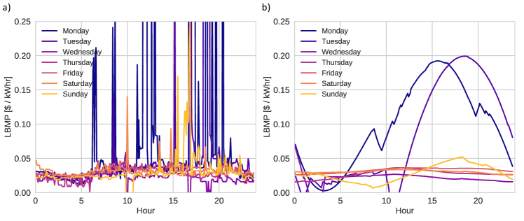
Over the past two decades, governments of 37 states, Washington D.C. and 4 territories across the United States have either put forward renewable portfolio standards or set renewable energy targets to address global warming.1 As a result, the contribution to energy production through renewable energy sources (RES) has increased and RES contributed 17.6% of the total electricity production in the United States in 20182. The intermittent nature of RES causes sudden changes in power availability which leads to demand and supply mismatch and thus electricity price fluctuations3. Figure 1 shows the variation in location based marginal price (LBMP) in New York City (NYC) for one week. LBMP is defined as the price of producing an additional MW of energy at a given time in a specific location4. In this paper, ‘electricity price’ and ‘LBMP’ are used synonymously. As seen in Figure 1a, the LBMP varies with the time of the day and it can be very low at some times of the day, even negative and as high as $1.2/kWh at some other times (not seen in Figure 1). This variation is more clearly seen in Figure 1b for Monday and Wednesday where the LBMP varies greatly throughout the day. Figure 1b is obtained by smoothing Figure 1a using the Savitzky Golay filter, which removes high frequency noise from the data while preserving the original shape of the data5. Smoothing the LBMP data makes it easy to observe the general structure of electricity prices on different days. It is seen that the price of electricity is, in general, higher on some days than the others.
Grid-scale energy storage is a suggested solution for electricity price management as it suppresses power output fluctuations and helps with peak load shaving6; 7. However, there are challenges in the deployment of large scale energy storage systems. These include technical challenges in integration of the storage facilities with the existing infrastructure, operational safety concerns associated with large scale storage facilities, and the high cost of storage systems.8; 9; 10. Vehicle-to-grid(V2G)11; 12 is a strategy studied here for distributed energy storage to supplement grid-scale storage to combat the problem of supply and demand mismatch.13 In V2G, participants use the electric vehicle (EV) battery to store energy during times of low demand and sell electricity back to the grid during times of high demand. With increased automobile electrification14 and increasing EV battery capacity15, V2G is now possible.
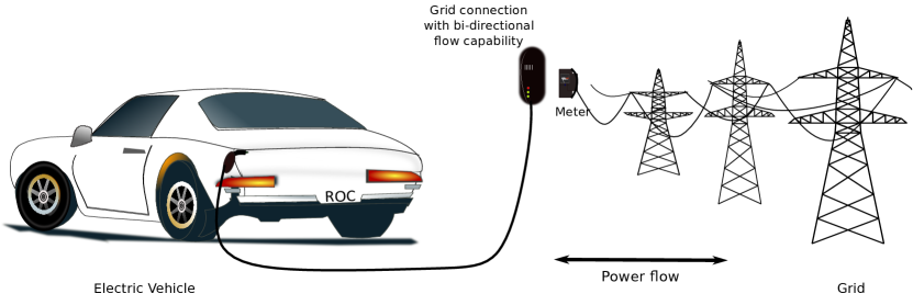
The procedure for a typical V2G operation is characterized by the following: (1) the EV battery is charged during off-peak hours, typically in the middle of the night; (2) the user commutes to work and uses a fraction of the battery capacity while doing so; (3) while the user is at work, the idle car is plugged into the grid at peak hours and electricity is sold to the grid based on whether the grid operator needs power; (4) some battery capacity is reserved to travel back home. After reaching home, the user repeats this cycle. Figure 2 shows a schematic of this operation.
The focus of this article is to assess the effect of battery performance metrics on the microeconomics of V2G implementation in the United States considering the randomness in EV owners’ driving patterns and realistic battery degradation. V2G needs infrastructure, like bidirectional energy and data flow between the electricity grid and the EVs, and vehicular design that allows availability of controls and metering on-board16; 11. Assuming that the infrastructure needed for V2G is already present, will a profit be created for EV owners’ if they participate in this program? What are the factors that will affect the savings they earn? How does V2G affect EV battery degradation? How does the charging/discharging rate and efficiency of the EV battery affect profits earned? Do commute patterns of EV users have any affect on V2G economics? A model is presented in this paper to answer these questions. Bayesian optimization is used to find the optimum conditions that will maximize EV owners’ benefits. The benefits for EV users are defined as the amount saved on electric fuel for mobility by participating in V2G.
Past research of V2G has studied technical, economical and commercial aspects.11; 17; 18; 19; 20; 21; 22; 23; 24 Overviews of challenges and benefits of V2G commercialization are presented by Sovacool and Hirsh 18; Mullan et al. 12 and Haidar et al. 25 Parsons et al. 26 and Sovacool et al. 24 present a systematic review of social challenges in V2G implementation. The work of Kuang et al. 27; Liu et al. 28 and Maigha and Crow 29 focuses on V2G scheduling and optimization. Kuang et al. 27 proposed an optimization model to study energy sharing between buildings and EV charging stations and the impact of driver behavior on V2G economic performance. Liu et al. 28 optimized dynamic dispatch of V2G microgrid systems using controlled charging and discharging while Maigha and Crow 29 proposed a day-ahead EV scheduling scheme to optimize V2G energy dispatch. An extensive review of different optimization techniques used in literature is presented by Tan et al. 23 V2G impact on the grid is examined in Guille and Gross 19; Druitt and Früh 30 and Chukwu and Mahajan 31. Guille and Gross 19 and Chukwu and Mahajan 31 both used aggregated vehicles for energy discharge and studied grid impact but Guille and Gross 19 focused more on the effectiveness of vehicle grid integration, while Chukwu and Mahajan 31 used mathematical modeling of V2G to quantify the amount of energy injected into the grid. The model by Druitt and Früh 30 simulated EVs to provide demand management and grid balancing services in the UK. Additionally, V2G implementation studies have been conducted in many locations to see how V2G would affect EV owners and electric operators. A summary of some of these studies is given in Table 1.
| Location | System Considerations | Findings | V2G Conclusion for Customer | V2G Conclusion for Grid |
| United Kingdom (UK) 32; 33; 34 | • An aggregated model of EVs that accounts for SOC, time of day, electricity prices and EV charging requirements • V2G scenarios with a decision making strategy for vehicle deployment • Analysis of benefits to the grid and cost savings to participating EV owners | • Minor impact of EVs on the distribution losses and voltage regulation of the grid • Commute cost reduced by half for EV owners | Strongly beneficial | Weakly disadvantageous |
| • Agent based coordinated dispatch strategy for EVs and renewable generators • Feasibility and stability of strategy tested on UK generic distribution system and EV owners’ profits calculated | • Average savings of EV owners is £1 per day which is not enough incentive for participation | Weakly beneficial | ||
| • Economic feasibility study of vehicle-to-building and V2G for ‘specific’ ancillary services • Accounts for vehicle trip data, electricity market pricing and triads and battery degradation | • Net present value of £8400 over 10 years is found to be the highest income generated by participation in the wholesale market and the capacity markets. • Major contributing factors are battery degradation, infrastructure costs, and electricity pricing | Strongly beneficial | ||
| Canary Islands, Spain 35 | • Cost benefit analysis of vehicle-to-home • Neglect battery degradation and benefits are calculated as savings in household energy bills | • Mobility energy cost of vehicle owners is reduced by 50 • Vehicle-to-home indirectly results in valley filling and peak shaving | Strongly beneficial | Strongly beneficial |
| Firenze, Italy 36 | • Model to design and size infrastructure for V2G integration using actual driving patterns • Focus on how energy demand changes with changing infrastructure, no economics | • V2G integration is capable of reducing 5% - 50% of daily electricity demand in some locations | Strongly beneficial | |
| Western Australia12 | • Utility scale economic analysis • V2G with plug-in hybrid EVs (PHEVs) for peak shaving, ancillary services, demand side management • Accounts for costs of infrastructure, and battery degradation | • V2G is not an economical option • Battery capital cost needs to significantly reduce for V2G to become economical for both individuals and industry | Weakly beneficial | Weakly beneficial |
| Canada 37 | • Policy adjustment scheme to optimize energy delivery through PHEV V2G aggregators for peak shaving • Accounts for randomness in vehicle mobility, battery degradation, and fixed time of use (TOU) pricing | • A state dependent policy works best for energy cost minimization of participating vehicles | Weakly beneficial | |
| Texas, United States (US) 38 | • Economic analysis of benefits of V2G with PHEVs for ancillary services to EV owners and the power system • Accounts for battery degradation cost and day ahead electricity pricing | • The cost savings to the power system are about 200 per vehicle in the PHEV fleet participating in ancillary service provision • Driving costs of vehicle owners are slightly reduced | Weakly beneficial | Strongly beneficial |
| New York City, US 16 | • Deterministic model analyzing economic benefits to an EV participant from V2G under different scenarios | • Maximum annual savings to the EV owner from the profitable scenarios range between 129 and 231 | Weakly beneficial |
From the Table 1, it is observed that early studies focused on using PHEVs for V2G. PHEVs have much lower energy capacity than EVs and thus, are capable of lower energy storage. Most of these studies consider the cost of battery degradation and electricity pricing data to analyze the economic benefits of V2G to vehicle owners or the power grid. In the work by Liang et al. 37, the starting time of commute and commute distance of vehicle owners are randomly sampled but this sampling is not supported by real data. The model by Gough et al. 34 is the only model that considers the stochasticity in driving patterns of EV owners but their economic analysis is for specific market conditions such as ancillary service provision during triads.iiiTriads are defined as the three half-hours of the highest demand on the Great Britain electricity transmission system between November and February each year. The price of electricity is on average ($50/kWh). This cannot be generalized for electricity markets around the world. The aim of this paper is to build a realistic model that does a cost-benefit analysis for V2G participants in different regions of the United States, taking into account historical electricity LBMP, realistic battery degradation, variable driving patterns and work schedules of EV drivers, and different EV models available in the market. A stochastic model for peak load shaving through V2G is presented. A deterministic model is one where results depend on selection of constraints and assumptions. In a stochastic model, randomness is introduced at different points in the model. In our model, electric cars (battery capacity) and user driving patterns and work schedules are randomized. To assess effects of battery performance metrics, we study the effect of charging/discharging rates under a realistic degradation model and extrapolate lithium-ion battery costs. In order to present the optimal scenario under randomness, we use Bayesian optimization, which provides an upper limit of real performance for maximizing benefits of EV users. Our results indicate that benefits are location dependent and users’ time of work matters most, among the randomized parameters, in determining the savings.
2 Methods
Our model calculates the profit of participating in the V2G scheme for EV owners in six cities of the United States using historic LBMP data and accounting for battery degradation and variable work and commute patterns of EV users. This stochastic model was constructed in PythoniiiiiiPython is a high level programming language with various scientific computing packages 39. and is designed to answer questions arising from the economics of V2G technology. LBMP varies throughout the day depending on the demand-supply dynamics and hence, the time of charging or discharging the vehicle affects the cost of charging the EV and profit earned from V2G. This makes it necessary to account for commute patterns and work hours of EV users to realistically calculate their economic benefits. There were 5298 EV users in New York City (NYC) as of December, 201940 and each of them may have different commute parameters leading to different savings from V2G. For example, savings from V2G may be different for an EV owner who works night shifts and an EV owner who typically works during the day since price of electricity is different during these times. The presented model jointly samples values for commute time and distance for every EV user from the data available from National Highway Travel Survey (NHTS, 2009) 41. The arrival times to work and hours worked per week are also sampled independently for every user from the American Community Survey data (ACS, 2016)42. The LBMP also varies by the day and to account for the impact of this daily variation on the benefits, vacation time of users is randomly sampled to be between 1-3 weeks. EV sales in United States increased 79% in 2018 from 2017 15 and with increased EV adoption, more automobile manufacturers have launched their electric car models. Thus, the model is designed to account for different EV models. 2019 United States EV sales data is used to sample EV models for V2G participants.
The model does a cost-benefit analysis for V2G participants under two scenarios as described by Freeman et al. 16 The price-taker scenario assumes that the user sells electricity whenever at work regardless of the cost of electricity at that time. Whereas the optimal selling price (OSP) scenario offers some control to each user by letting them fix a selling price at the start of every year and electricity is sold if the LBMP is greater than that fixed price. So, while at work, the EV is plugged-in to the grid but energy is sold only when LBMP at a given time exceeds the user-defined OSP. In a ’mean model’, each user in a particular city would have the same OSP which may lead to losses for some users since the costs incurred by them may exceed the cost of commute. Hence, OSP for each user is optimized such that profits from V2G are maximized. Bayesian optimization43 was used to optimize the selling price for each user. LBMP data is obtained from Independent System Operators4; 44; 45; 46 i.e. the operators for competitive wholesale markets in the different states.
The probability distribution for making a net annual profit of by participation in V2G by an EV owner can be calculated from the joint probability of and the vector and converting it to a conditional probability as in Equation (1). is a vector of the model constants and random variables . is the conditional probability of earning a net annual profit given . The integral in Equation (1) is over the sample space of . Since, are fixed parameters, they do not affect . For a particular set of stochastic variables , becomes deterministic and is written as . is given by Equation (4).
| (1) |
and are defined in Equations (2) and (3), respectively.
| (2) |
| (3) |
is depth of discharge, is the one way efficiency of charging/discharging, is the rate of charging, is the rate of discharging, is the commute time, is the commute distance of the EV user, is the time of work, is the number of hours worked by the user, and is the battery capacity in kWh depending on the EV model.
| (4) |
is a time integral and it depends on power charged or discharged in at a given time , the LBMP at that time in , the differential battery degradation cost for the power transacted, in . V2G activity is assumed to be done only on working days and the US Federal Calendar is used to determine the holidays. is defined in Equation (5) as a combination of Heaviside step functions which determine the power discharged or charged when the EV is plugged in into the grid.
| (5) |
Where is the energy capacity used to commute. and are the rates of charging and discharging, respectively and are treated equal at 11.5kW assuming that a J1772 level 2 charger is used for all charging and discharging purposes. As determined by Apostolaki-Iosifidou et al. 47, a round-trip efficiency of 70% is used for determination of charging and discharging costs of the EV owners. Hence, is assumed to be 83.7%, the square root of the round trip efficiency 70% 47. Discharging the battery to 100% depth (called deep discharge) accelerates the degradation process and less the , the better it is for the battery lifetime48. The DoD for this model is fixed to be 90% so that battery degradation is not accelerated but there is enough battery capacity that can be used for commute and V2G. State of Charge (SoC) of the battery is an important consideration when charging or discharging because the EV battery must not be overcharged or discharged in excess of what can be sold at any given time. It is calculated as a time integral of .
| (6) |
is a control function used to ensure that electricity is sold only if LBMP is greater than the set selling price, , at any given time .
| (7) |
| (8) |
and are time dependent indicator functions that indicate the state of the EV user as ‘at work’ or ‘at home’, respectively. The charging or discharging of EVs is also dependent on state of the user at a given time besides the SoC of EV battery at that time. If the EV user is at work, the EV is said to be discharging (selling electricity) and if at home, the EV is said to be charging (buying electricity).
| (9) |
| (10) |
| (11) |
where is the time of work and is also treated as the start time for discharging, is the commute time in hours, and is the time when user arrives home from work and is treated as charging start time. is sampled stochastically from data42 :
| (12) |
‘’ indicates that samples were drawn probabilistically. The energy needed for commute, is calculated as
| (13) |
where is the commute distance in miles and is the rated range of the vehicle in miles. is sampled stochastically from the 2016 EV sales data and the rated range of an EV is provided by the EPA49.
| (14) |
The NHTS dataset 41 is used to jointly sample the commute time and commute distance for the EV users.
| (15) |
Finally, the probability of earning savings, S, from V2G is calculated as the probability of difference between the total profit from charging/discharging that the EV owner earns while participating in V2G, , and the total profit the user earns for normal commute without V2G, .
| (16) |
The profit for commute only scenario is calculated in a similar fashion as V2G except that there is no selling of electricity. The duration of charging differs for commute only and V2G scenario because the energy capacity used throughout the day is different in both scenarios.
One important factor that contributes to the total cost to EV users is the battery degradation cost, . Battery degradation is the gradual loss of capacity over the lifetime of a battery. Accurately modeling the battery degradation is relatively difficult because there are a variety of hypothesized mechanisms that reduce capacities of batteries and each is specific to the cathode, anode, and electrolyte choice50. An overview of the state-of-the art in lithium ion battery degradation modeling is given in the work by Thompson 51. The EV battery undergoes wear not only due to additional charge/discharge cycles (cycle aging) but also when the battery is resting (calendar aging)52. Temperature (), SoC, DoD and number of cycles () are the factors that contribute to battery degradation53. In this work, a modified version of the semiempirical lifetime prediction model developed by National Renewable energy Laboratory (NREL)54; 48 is used. This model takes into account all the above mentioned factors to estimate the battery capacity fade due to calendar aging as well as cycle aging. Capacity fade due to calendar aging is dominated by solid-electrolyte interphase growth resulting in loss of cyclable lithium while that due to cycle aging is controlled by active material loss and mechanical failure54; 48. Equations (17) – (19) are the governing equations for capacity fade.
| (17) |
| (18) |
| (19) |
Where gives the capacity fade at time . and are the calendar aging and cycle aging components, respectively, of battery capacity fade. Coefficients are degradation rate constants that depend on the aging condition of battery. Details of the model can be found in Santhanagopalan et al. 48
The battery degradation cost at a given time is then calculated from capacity fade using Equation (20).
| (20) |
where is the capital cost of the battery in $/kWh. gives the battery degradation in kWh because obtained from Equation (19) is the relative battery capacity left after degradation. We introduce SF which is the saturation factor and is defined as the percentage degradation after which the EV battery needs to be replaced.
The above stochastic model was implemented for commuting EV owners participating in V2G in six US cities with real commuting data. A discussion of results is presented in the next section.
3 Results and Discussion
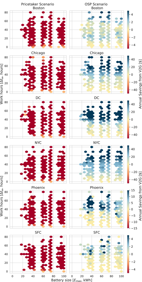
It is found that OSP scenario produces positive savings for the EV users while the price-taker scenario adds to the existing commute cost and makes V2G unprofitable. The variance in the magnitude of savings in both scenarios comes from the randomness introduced in the selection of EV models, and charging and discharging time due to the randomness in commute parameters and work patterns. We find that, in all cities, time of work significantly impacts the magnitude of savings. The effect of charging rate, and battery efficiency on V2G savings was also studied along with the effect of battery capital cost. While charging rate is found to be a crucial factor in increasing savings, battery capital cost is found to have little effect on V2G savings.
3.1 V2G Economics in Different Cities
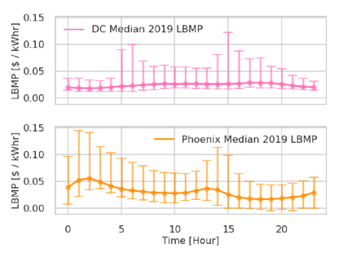
Commute patterns and electricity prices change from one city to the other. To see how V2G economics change with changing commute patterns and LBMPs, the economic analysis is applied to the cities of Boston, Chicago, Washington DC (DC), NYC, Phoenix, and San Francisco City (SFC). The commute parameters are sampled for each city using the ACS42 and NHTS41 datasets. 2019 LBMP data for respective cities are used to calculate the profitability of V2G. The LBMP for different cities was acquired from the local electric power markets45; 44; 4; 46. The electricity pricing data is available on the websites of these electric market operators and the model uses historic TOU LBMP data for all the cities. Figure 3 shows the difference in LBMP for DC and Phoenix as an example. The LBMP in Phoenix, on average, rises between 1pm and 4pm and again between 12am and 5am. However, in DC, the median LBMP is nearly constant throughout the day. Such differences in LBMP are also observed for other cities.
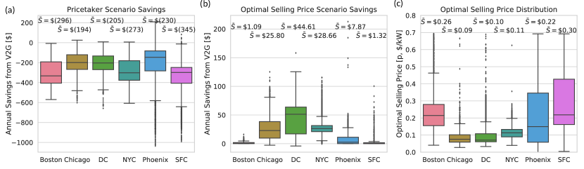
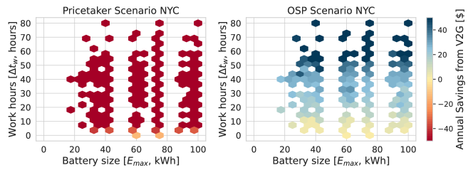
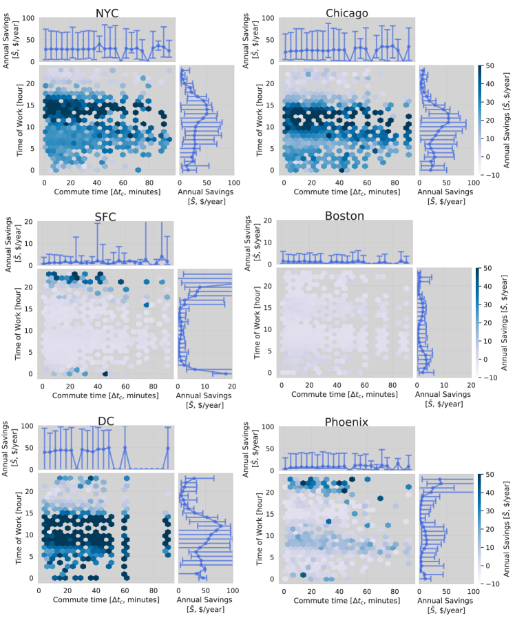
The results in Figure 4 illustrate economics of V2G in different cities. There is no profit in the price-taker scenario and the users spend more by participating in V2G. This is seen in Figure 4a. In the OSP scenario, users in all cities have positive savings because the OSP, , is optimized so that the total cost to the users is less than the cost borne for commute without V2G (Figure 4b). The maximum possible annual savings vary by city. Figure 4c shows the distribution of OSP, , for the six cities in consideration. The general structure of LBMP throughout the day and the number of work hours per week play a major role in determining the average distribution of OSP. It is found that EV owners having who work fewer than 5 hours per week have osp of $0/kWh and those working fewer than 10 hours have close to zero savings. The correlation between savings and number of working hours is illustrated in Figure 5 for NYC. When the number of working hours is small, the window for selling for V2G is short and results in smaller or no savings. In general, potential for savings increases with the number of weekly working hours. On the other hand, battery size has little effect on savings. Figure S2 shows this variation for the other cities. Boston and SFC have low savings but a similar correlation with the number of working hours is observed.
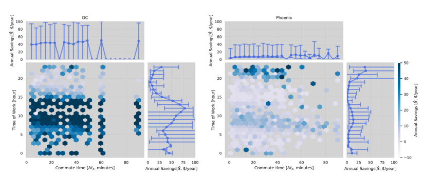
The variation in savings in different cities comes from the fact that commute patterns and work patterns differ in these cities. Profit favouring time of work is significant for high annual savings besides the average weekly working hours. In Figure 3, it is seen that the LBMP in Phoenix is low during most hours except early afternoon and late night. Hence, the EV users going to work during those peak hours are likely to make bigger savings while EV users going to work other than those peak hours have smaller savings in Phoenix. This can further be seen in Figure 6 which compares the effect of commute time and time of work on the annual savings in DC and Phoenix. Notice that the EV users in Phoenix make greater savings if they start work between 8 pm and 2 am. The commute time doesn’t seem to have as much effect on the annual savings as the time of work. Savings in DC are highest for start time of work between 8 am and 3 pm and very low between 5 pm and 11 pm which is also consistent with the LBMP pattern for DC seen in Figure 3. Figure S1 shows savings as a function of time of work and commute time for other cities. NYC and Chicago have a similar distribution of savings like DC and the higher savings are observed for time of work between 10 am and 4 pm. In Boston, though the magnitude of savings is low generally, two bands of higher savings are observed for time of work between 1 am and 5 am, and between 11 am and 4 pm. The LBMP distribution in SFC is much like Phoenix, higher at night than in the day. Consequently, the savings in SFC are highest between 6 pm and 1 am. This shows how important LBMP and time of work are in determining V2G savings.
3.2 Effect of Battery Efficiency and Charging Rates on V2G Savings
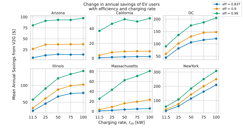
Charging efficiency is shown to have an effect on charging and discharging power losses55; 56; 57. Studies are aimed at improving efficiency of lithium-ion batteries and finding new energy efficient materials 58. The current one-way efficiency of lithium-ion batteries is 83.7% 47. V2G analysis for higher efficiencies of 90% and 99% was done and compared to the current 83.7% to see how the increasing efficiency would affect the annual V2G savings. Figure 7 shows the results for this analysis. It is observed that as efficiency increases, V2G savings increase as the power losses during charging and discharging are cut down. Few studies have also demonstrated the effect of varying charging rates on profits to EV owners. Andersson et al. 59 studied the effect of increasing charging rates on V2G (using PHEVs) for providing regulatory power in Sweden and Germany. They observed a four fold increase in PHEV users’ profits when the charging rate was increased from 3.3kW to 15kW. Hence, the savings obtained at different efficiencies are also compared at various charging rates and higher charging rates result in increased savings from V2G. It can be seen in Figure 7 that increasing the charging rate results in an increase in savings which is consistent with findings of Andersson et al. 59
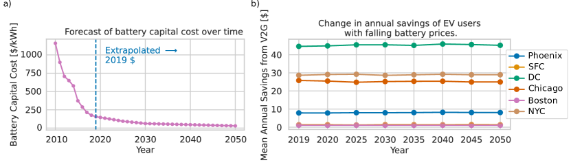
3.3 Future Battery Capital Costs and V2G
The cost of lithium-ion batteries, which are most commonly used in EVs, has been falling and is projected to fall further from the current $156/kWh to $94/kWh by 2025 and to $62/kWh by 2030 (Figure 8a).60; 61; 14 Will the falling price of batteries have any impact on savings earned from V2G at the current electricity prices? To answer this question, lithium-ion battery costs are extrapolated using exponential fitting up to 2050 and V2G economics calculated for every year for all cities previously mentioned. Current LBMPs and driving patterns are kept constant over the years and only battery capital cost is varied for these calculations. The OSP is optimized for every year. Figure 8 shows how the mean savings change with the change in the battery capital cost over the years. Savings remain almost constant for all cities as the battery prices fall indicating that battery cost has little effect.
3.4 Comparison with related work
The results of this paper were compared with similar studies and conclusions were found to be similar in some cases. In the strategies proposed by Wang et al. 33; Ma et al. 32; Colmenar-Santos et al. 35, they observe that V2G effectively reduces mobility fuel cost if EV charging and discharging is done smartly. Colmenar-Santos et al. 35 use ‘dumb-charging’ versus ‘smart-charging’ scenarios to calculate benefits from vehicle-to-home in Canary islands and find that the annual savings of users compared to just commute are ($103) in the ‘dumb-charging’ case and ($165) in the ‘smart-charging’ case. The dumb- and smart-charging cases used by them are analogous to the price-taker and OSP scenario in this paper but the scenarios in Colmenar-Santos et al. 35 consider that the transactions are not happening over the meter. The techno-economic study by Dufo-López and Bernal-Agustín 62 concluded that V2G storage system is not profitable for consumers in Spain at the current battery costs. They conclude that the battery capital cost must decrease and battery efficiency must improve before V2G is profitable to EV users in Spain. In contrast to these findings, Gough et al. 34 claim that using V2G in the UK, if used for capacity markets, will make savings as high as ($10300) in a 10 year period and these savings are said to account for the infrastructure cost. These large savings are possible in the UK due to the annual triads. This verifies the finding that profits from V2G are location dependent. In the current study, there are some EV users who save around $120/year – $150/year which is close to the findings of Gough et al. 34
4 Conclusions
A stochastic model with a realistic degradation model, and empirical driving and work patterns was built to assess effects of battery performance on EV users’ profits from V2G. EV charging rate plays a crucial role in V2G profitability from a microeconomic point of view. The effect of efficiency, charging rates, and battery capital cost on V2G savings was studied. Two economic scenarios were evaluated - price-taker scenario and an optimal selling price scenario. Giving users a choice to set a selling price is crucial to make V2G a profitable scheme. Savings from V2G are highly location dependent due to a difference in electricity pricing. We find that an increasing charging rate and efficiency are much more important than the capital cost of lithium-ion batteries across all cities. Therefore, focusing future research efforts toward increasing EV charging rates and efficiency is more important than increasing EV battery capacity for V2G or cycle lifetime.
5 Acknowledgement
Authors would like to thank Center for Integrated Research Computing (CIRC) for providing computational resources and technical support. This research did not receive any specific grant from funding agencies in the public, commercial, or not-for-profit sectors.
References
- Durkay [2021] Jocelyn Durkay. State renewable portfolio and standards, 2021. URL http://www.ncsl.org/research/energy/renewable-portfolio-standards.aspx.
- Office of Energy Efficiency & Renewable Energy [2018] Office of Energy Efficiency & Renewable Energy. 2018 Renewable Energy Data Book. Technical report, US DOE, 2018. URL https://www.nrel.gov/docs/fy20osti/75284.pdf.
- Daina et al. [2017] Nicolò Daina, Aruna Sivakumar, and John W. Polak. Electric vehicle charging choices: Modelling and implications for smart charging services. Transp. Res. Part C Emerg. Technol., 81:36–56, aug 2017. ISSN 0968-090X. doi:10.1016/J.TRC.2017.05.006. URL https://www.sciencedirect.com/science/article/pii/S0968090X17301365?via{%}3Dihub.
- [4] New York ISO. URL http://www.nyiso.com/.
- Savitzky and Golay [1951] Abraham Savitzky and Marcel J. E. Golay. Smoothing and Differentiation of Data by Simplified Least Squares Procedures. Anal. Chem., 36(8):1627–1639, 1951. doi:10.1021/ac60214a047. URL https://pubs.acs.org/sharingguidelines.
- Castillo and Gayme [2014] Anya Castillo and Dennice F. Gayme. Grid-scale energy storage applications in renewable energy integration: A survey. Energy Convers. Manag., 87:885–894, nov 2014. ISSN 01968904. doi:10.1016/j.enconman.2014.07.063. URL https://linkinghub.elsevier.com/retrieve/pii/S0196890414007018.
- Zame et al. [2018] Kenneth K. Zame, Christopher A. Brehm, Alex T. Nitica, Christopher L. Richard, and Gordon D. Schweitzer III. Smart grid and energy storage: Policy recommendations. Renew. Sustain. Energy Rev., 82:1646–1654, feb 2018. ISSN 13640321. doi:10.1016/j.rser.2017.07.011. URL https://linkinghub.elsevier.com/retrieve/pii/S1364032117310663.
- IRENA [2017] IRENA. Electricity Storage and Renewables: Costs and Markets to 2030. International Renewable Energy Agency, Abu Dhabi, 2017. ISBN 9789292600389. URL www.irena.org.
- USG [2018] Energy Storage: Information on Challenges to Deployment for Electricity Grid Operations and Efforts to Address Them Report. Technical report, United States Government Accountability Office, 2018. URL https://www.gao.gov/assets/700/691983.pdf.
- Sharma and Sharma [2019] Angshuman Sharma and Santanu Sharma. Review of power electronics in vehicle-to-grid systems. Journal of Energy Storage, 21:337–361, 2019. ISSN 2352-152X. doi:https://doi.org/10.1016/j.est.2018.11.022. URL http://www.sciencedirect.com/science/article/pii/S2352152X1830481X.
- Kempton and Tomić [2005a] Willett Kempton and Jasna Tomić. Vehicle-to-grid power implementation: From stabilizing the grid to supporting large-scale renewable energy. J. Power Sources, 144(1):280–294, jun 2005a. ISSN 0378-7753. doi:10.1016/J.JPOWSOUR.2004.12.022. URL https://www.sciencedirect.com/science/article/pii/S0378775305000212?via{%}3Dihub.
- Mullan et al. [2012] Jonathan Mullan, David Harries, Thomas Bräunl, and Stephen Whitely. The technical, economic and commercial viability of the vehicle-to-grid concept. Energy Policy, 48:394–406, sep 2012. ISSN 0301-4215. doi:10.1016/J.ENPOL.2012.05.042. URL https://www.sciencedirect.com/science/article/pii/S0301421512004545.
- Wang and Wang [2013] Zhenpo Wang and Shuo Wang. Grid power peak shaving and valley filling using vehicle-to-grid systems. IEEE Transactions on Power Delivery, 28(3):1822–1829, 2013.
- McK [2017] Electrifying insights: How automakers can drive electrified vehicle sales and profitability. Technical report, McKinsey & Company, January 2017. URL https://www.mckinsey.com/industries/automotive-and-assembly/our-insights.
- EV_[2017] Global ev outlook 2017. Technical report, International Energy Agency, January 2017. URL www.iea.org.
- Freeman et al. [2017] Gerad M. Freeman, Thomas E. Drennen, and Andrew D. White. Can parked cars and carbon taxes create a profit? The economics of vehicle-to-grid energy storage for peak reduction. Energy Policy, 106:183–190, jul 2017. ISSN 0301-4215. doi:10.1016/J.ENPOL.2017.03.052. URL https://www.sciencedirect.com/science/article/pii/S0301421517302070?via{%}3Dihub.
- Kempton and Tomić [2005b] Willett Kempton and Jasna Tomić. Vehicle-to-grid power fundamentals: Calculating capacity and net revenue. J. Power Sources, 144(1):268–279, jun 2005b. ISSN 0378-7753. doi:10.1016/J.JPOWSOUR.2004.12.025. URL https://www.sciencedirect.com/science/article/pii/S0378775305000352?via{%}3Dihub.
- Sovacool and Hirsh [2009] Benjamin K. Sovacool and Richard F. Hirsh. Beyond batteries: An examination of the benefits and barriers to plug-in hybrid electric vehicles (PHEVs) and a vehicle-to-grid (V2G) transition. Energy Policy, 37(3):1095–1103, mar 2009. ISSN 0301-4215. doi:10.1016/J.ENPOL.2008.10.005. URL https://www.sciencedirect.com/science/article/pii/S0301421508005934.
- Guille and Gross [2009] Christophe Guille and George Gross. A conceptual framework for the vehicle-to-grid (V2G) implementation. Energy Policy, 37(11):4379–4390, nov 2009. ISSN 0301-4215. doi:10.1016/J.ENPOL.2009.05.053. URL https://www.sciencedirect.com/science/article/pii/S0301421509003978.
- Sortomme and El-Sharkawi [2011] Eric Sortomme and Mohamed A. El-Sharkawi. Optimal Charging Strategies for Unidirectional Vehicle-to-Grid. IEEE Trans. Smart Grid, 2(1):131–138, mar 2011. ISSN 1949-3053. doi:10.1109/TSG.2010.2090910. URL http://ieeexplore.ieee.org/document/5661888/.
- Ehsani et al. [2012] Mehrdad Ehsani, Milad Falahi, Saeed Lotfifard, Mehrdad Ehsani, Milad Falahi, and Saeed Lotfifard. Vehicle to Grid Services: Potential and Applications. Energies, 5(10):4076–4090, oct 2012. ISSN 1996-1073. doi:10.3390/en5104076. URL http://www.mdpi.com/1996-1073/5/10/4076.
- Liu et al. [2013] Chunhua Liu, K. T. Chau, Diyun Wu, and Shuang Gao. Opportunities and Challenges of Vehicle-to-Home, Vehicle-to-Vehicle, and Vehicle-to-Grid Technologies. Proc. IEEE, 101(11):2409–2427, nov 2013. ISSN 0018-9219. doi:10.1109/JPROC.2013.2271951. URL http://ieeexplore.ieee.org/document/6571224/.
- Tan et al. [2016] Kang Miao Tan, Vigna K. Ramachandaramurthy, and Jia Ying Yong. Integration of electric vehicles in smart grid: A review on vehicle to grid technologies and optimization techniques. Renew. Sustain. Energy Rev., 53:720–732, jan 2016. ISSN 1364-0321. doi:10.1016/J.RSER.2015.09.012. URL https://www.sciencedirect.com/science/article/pii/S136403211500982X?via{%}3Dihub.
- Sovacool et al. [2018] Benjamin K Sovacool, Lance Noel, Jonn Axsen, and Willett Kempton. The neglected social dimensions to a vehicle-to-grid (V2G) transition: a critical and systematic review. Environ. Res. Lett., 13(1):013001, jan 2018. ISSN 1748-9326. doi:10.1088/1748-9326/aa9c6d. URL http://stacks.iop.org/1748-9326/13/i=1/a=013001?key=crossref.9203e40373b5f1d7115356d673378c1b.
- Haidar et al. [2014] Ahmed M.A. Haidar, Kashem M. Muttaqi, and Danny Sutanto. Technical challenges for electric power industries due to grid-integrated electric vehicles in low voltage distributions: A review. Energy Convers. Manag., 86:689–700, oct 2014. ISSN 0196-8904. doi:10.1016/J.ENCONMAN.2014.06.025. URL https://www.sciencedirect.com/science/article/pii/S0196890414005500.
- Parsons et al. [2014] George R. Parsons, Michael K. Hidrue, Willett Kempton, and Meryl P. Gardner. Willingness to pay for vehicle-to-grid (V2G) electric vehicles and their contract terms. Energy Econ., 42(C):313–324, mar 2014. doi:10.1016/j.eneco.2013.12.018. URL https://linkinghub.elsevier.com/retrieve/pii/S0140988314000024.
- Kuang et al. [2017] Yanqing Kuang, Yang Chen, Mengqi Hu, and Dong Yang. Influence analysis of driver behavior and building category on economic performance of electric vehicle to grid and building integration. Appl. Energy, 207:427–437, dec 2017. ISSN 0306-2619. doi:10.1016/J.APENERGY.2017.07.006. URL https://www.sciencedirect.com/science/article/pii/S030626191730870X?via{%}3Dihub.
- Liu et al. [2015] Haitao Liu, Yu Ji, Huaidong Zhuang, Hongbin Wu, Haitao Liu, Yu Ji, Huaidong Zhuang, and Hongbin Wu. Multi-Objective Dynamic Economic Dispatch of Microgrid Systems Including Vehicle-to-Grid. Energies, 8(5):4476–4495, may 2015. ISSN 1996-1073. doi:10.3390/en8054476. URL http://www.mdpi.com/1996-1073/8/5/4476.
- Maigha and Crow [2017] Maigha and Mariesa L. Crow. Multi-objective electric vehicle scheduling considering customer and system objectives. In 2017 IEEE Manchester PowerTech, pages 1–6. IEEE, jun 2017. ISBN 978-1-5090-4237-1. doi:10.1109/PTC.2017.7981275. URL http://ieeexplore.ieee.org/document/7981275/.
- Druitt and Früh [2012] James Druitt and Wolf-Gerrit Früh. Simulation of demand management and grid balancing with electric vehicles. J. Power Sources, 216:104–116, oct 2012. ISSN 03787753. doi:10.1016/j.jpowsour.2012.05.033. URL https://linkinghub.elsevier.com/retrieve/pii/S0378775312008907.
- Chukwu and Mahajan [2017] Uwakwe C. Chukwu and Satish M. Mahajan. Modeling of V2G net energy injection into the grid. In 2017 6th Int. Conf. Clean Electr. Power, pages 437–440. IEEE, jun 2017. ISBN 978-1-5090-4682-9. doi:10.1109/ICCEP.2017.8004724. URL http://ieeexplore.ieee.org/document/8004724/.
- Ma et al. [2012] Yuchao Ma, Tom Houghton, Andrew Cruden, and David Infield. Modeling the Benefits of Vehicle-to-Grid Technology to a Power System. IEEE Trans. Power Syst., 27(2):1012–1020, may 2012. ISSN 0885-8950. doi:10.1109/TPWRS.2011.2178043. URL http://ieeexplore.ieee.org/document/6123186/.
- Wang et al. [2016] Lu Wang, Suleiman Sharkh, and Andy Chipperfield. Optimal coordination of vehicle-to-grid batteries and renewable generators in a distribution system. Energy, 113:1250–1264, oct 2016. ISSN 0360-5442. doi:10.1016/J.ENERGY.2016.07.125. URL https://www.sciencedirect.com/science/article/pii/S0360544216310490.
- Gough et al. [2017] Rebecca Gough, Charles Dickerson, Paul Rowley, and Chris Walsh. Vehicle-to-grid feasibility: A techno-economic analysis of EV-based energy storage. Appl. Energy, 192:12–23, apr 2017. ISSN 0306-2619. doi:10.1016/J.APENERGY.2017.01.102. URL https://www.sciencedirect.com/science/article/pii/S0306261917301149?via{%}3Dihub.
- Colmenar-Santos et al. [2017] A. Colmenar-Santos, Carlos de Palacio-Rodriguez, Enrique Rosales-Asensio, and David Borge-Diez. Estimating the benefits of vehicle-to-home in islands: The case of the Canary Islands. Energy, 134:311–322, sep 2017. ISSN 0360-5442. doi:10.1016/J.ENERGY.2017.05.198. URL https://www.sciencedirect.com/science/article/pii/S0360544217309647.
- De Gennaro et al. [2015] Michele De Gennaro, Elena Paffumi, and Giorgio Martini. Customer-driven design of the recharge infrastructure and Vehicle-to-Grid in urban areas: A large-scale application for electric vehicles deployment. Energy, 82:294–311, mar 2015. ISSN 0360-5442. doi:10.1016/J.ENERGY.2015.01.039. URL https://www.sciencedirect.com/science/article/pii/S0360544215000638.
- Liang et al. [2013] Hao Liang, Bong Jun Choi, Weihua Zhuang, and Xuemin Shen. Optimizing the Energy Delivery via V2G Systems Based on Stochastic Inventory Theory. IEEE Trans. Smart Grid, 4(4):2230–2243, dec 2013. ISSN 1949-3053. doi:10.1109/TSG.2013.2272894. URL http://ieeexplore.ieee.org/document/6566201/.
- Sioshansi and Denholm [2010] Ramteen Sioshansi and Paul Denholm. The Value of Plug-In Hybrid Electric Vehicles as Grid Resources. 31(3):1–23, 2010. URL https://www.jstor.org/stable/41323291.
- Oliphant [2015] Travis E. Oliphant. A guide to NumPy, 2015. URL https://www.numpy.org/.
- nys [2020] Electric vehicle registration map - nyserda, 2020. URL https://www.nyserda.ny.gov/All-Programs/Programs/ChargeNY/Support-Electric/Map-of-EV-Registrations.
- NHT [2017] NHTS Dataset, US Department of Transportation Federal Highway Administration, 2017. URL http://nhts.ornl.gov.
- PUM [2016] PUMS Data, American Community Survey, U.S. Census Bureau, 2016. URL https://www.census.gov/programs-surveys/acs/data/pums.html.
- Jones et al. [1998] Donald R. Jones, Matthias Schonlau, and William J. Welch. Efficient Global Optimization of Expensive Black-Box Functions. J. Glob. Optim., 13(4):455–492, 1998. ISSN 09255001. doi:10.1023/A:1008306431147. URL https://link.springer.com/article/10.1023/A:1008306431147.
- [44] ISO New England. URL http://www.iso-ne.com/.
- [45] California ISO. URL http://www.caiso.com/.
- [46] PJM Interconnection. URL http://www.pjm.com/.
- Apostolaki-Iosifidou et al. [2018] Elpiniki Apostolaki-Iosifidou, Willett Kempton, and Paul Codani. Reply to Shirazi and Sachs comments on “Measurement of Power Loss During Electric Vehicle Charging and Discharging”. Energy, 142:1142–1143, 2018. ISSN 0360-5442. doi:https://doi.org/10.1016/j.energy.2017.10.080. URL http://www.sciencedirect.com/science/article/pii/S0360544217317851.
- Santhanagopalan et al. [2015] Shriram Santhanagopalan, Gi-Heon Kim, Matthew Keyers, Ahmad A. Pesaran, Kandler Smith, and Jeremy Neubauer. Design and analysis of large lithium-Ion battery systems. Artech House, 2015. ISBN 9781608077137. URL https://us.artechhouse.com/Design-Analysis-of-Large-Lithium-Ion-Battery-Systems-P1705.aspx.
- [49] US EPA. Green Vehicle Guide - Explaining Electric & Plug-In Hybrid Electric Vehicles. URL https://www.epa.gov/greenvehicles/explaining-electric-plug-hybrid-electric-vehicles.
- Kabir and Demirocak [2017] M. M. Kabir and Dervis Emre Demirocak. Degradation mechanisms in Li-ion batteries: a state-of-the-art review. Int. J. Energy Res., 41(14):1963–1986, nov 2017. ISSN 0363907X. doi:10.1002/er.3762. URL http://doi.wiley.com/10.1002/er.3762.
- Thompson [2018] Andrew W. Thompson. Economic implications of lithium ion battery degradation for Vehicle-to-Grid (V2X) services. J. Power Sources, 396:691–709, aug 2018. ISSN 0378-7753. doi:10.1016/J.JPOWSOUR.2018.06.053. URL https://www.sciencedirect.com/science/article/pii/S0378775318306499.
- Keil et al. [2016] Peter Keil, Simon F. Schuster, Jörn Wilhelm, Julian Travi, Andreas Hauser, Ralph C. Karl, and Andreas Jossen. Calendar Aging of Lithium-Ion Batteries. J. Electrochem. Soc., 163(9):A1872–A1880, jul 2016. ISSN 0013-4651. doi:10.1149/2.0411609jes. URL http://jes.ecsdl.org/lookup/doi/10.1149/2.0411609jes.
- Smith et al. [2017] Kandler Smith, Aron Saxon, Matthew Keyser, Blake Lundstrom, Ziwei Cao, and Albert Roc. Life prediction model for grid-connected Li-ion battery energy storage system. In 2017 Am. Control Conf., pages 4062–4068. IEEE, may 2017. ISBN 978-1-5090-5992-8. doi:10.23919/ACC.2017.7963578. URL http://ieeexplore.ieee.org/document/7963578/.
- Smith et al. [2012] Kandler Smith, Matthew Earleywine, Eric Wood, Jeremy Neubauer, and Ahmad Pesaran. Comparison of Plug-In Hybrid Electric Vehicle Battery Life Across Geographies and Drive Cycles. In SAE Tech. Pap. SAE International, 2012. doi:10.4271/2012-01-0666. URL https://doi.org/10.4271/2012-01-0666.
- Apostolaki-Iosifidou et al. [2017] Elpiniki Apostolaki-Iosifidou, Paul Codani, and Willett Kempton. Measurement of power loss during electric vehicle charging and discharging. Energy, 127:730–742, may 2017. doi:10.1016/j.energy.2017.03.015. URL https://linkinghub.elsevier.com/retrieve/pii/S0360544217303730.
- Eftekhari [2017] Ali Eftekhari. Energy efficiency: a critically important but neglected factor in battery research. Sustain. Energy Fuels, 1(10):2053–2060, nov 2017. doi:10.1039/C7SE00350A. URL http://xlink.rsc.org/?DOI=C7SE00350A.
- Li and Tseng [2015] Kaiyuan Li and King Jet Tseng. Energy efficiency of lithium-ion battery used as energy storage devices in micro-grid. In IECON 2015 - 41st Annu. Conf. IEEE Ind. Electron. Soc., pages 005235–005240. IEEE, nov 2015. ISBN 978-1-4799-1762-4. doi:10.1109/IECON.2015.7392923. URL http://ieeexplore.ieee.org/document/7392923/.
- Few et al. [2018] Sheridan Few, Oliver Schmidt, Gregory J. Offer, Nigel Brandon, Jenny Nelson, and Ajay Gambhir. Prospective improvements in cost and cycle life of off-grid lithium-ion battery packs: An analysis informed by expert elicitations. Energy Policy, 114:578–590, mar 2018. ISSN 03014215. doi:10.1016/j.enpol.2017.12.033. URL https://linkinghub.elsevier.com/retrieve/pii/S0301421517308595.
- Andersson et al. [2010] S.-L. Andersson, A.K. K Elofsson, M.D. D Galus, L. Göransson, S. Karlsson, F. Johnsson, and G. Andersson. Plug-in hybrid electric vehicles as regulating power providers: Case studies of Sweden and Germany. Energy Policy, 38(6):2751–2762, jun 2010. ISSN 0301-4215. doi:10.1016/J.ENPOL.2010.01.006. URL https://www.sciencedirect.com/science/article/pii/S0301421510000121.
- Bloomberg New Energy Finance [2020] Bloomberg New Energy Finance. Electric vehicle outlook 2020. Technical report, Bloomberg, 2020. URL https://about.bnef.com/electric-vehicle-outlook/.
- Citi GPS [2016] Citi GPS. Investment themes in 2016. Technical report, Citigroup, January 2016. URL https://www.citi.com/commercialbank/insights/assets/docs/investment-themes-in-2016.pdf.
- Dufo-López and Bernal-Agustín [2015] Rodolfo Dufo-López and José L. Bernal-Agustín. Techno-economic analysis of grid-connected battery storage. Energy Convers. Manag., 91:394–404, feb 2015. ISSN 01968904. doi:10.1016/j.enconman.2014.12.038. URL https://linkinghub.elsevier.com/retrieve/pii/S0196890414010772.
Supplemental Information: City-wide modeling of Vehicle-to-Grid Economics to Understand Effects of Battery Performance
S1 Savings and work patterns