Hong Kong Air Traffic: Explanation and Prediction based on Sparse Seasonal ARIMA Model

Shuwen Chai
School of Statistics
Renmin University of China
chaishuwen@ruc.edu.cn

Abstract

The monthly air traffic of a city is a time series with obvious seasonal pattern, and is closely related to the economic situation and social environment of the city. In Hong Kong, for example, July, August and October tend to be the peak season of traffic flow, while there is also a relatively fixed off-season. In the case of a stable social environment, a carefully identified and fitted seasonal ARIMA model can predict the traffic flow in the future months well. This work selects the air traffic data, including arrival and departure passengers of Hong Kong, after the financial crisis and before the political storm. A sparse seasonal ARIMA $(0,1,1)\times(4,1,0)_{12}$ is built, which can correctly predict the air traffic from January to July in 2020 within its $95\%$ confidence interval. Furthermore, this work decompose the time-series and find that important events, like financial crisis, political storm, and the COVID-19 outbreak, affect the level of air traffic to some extent. For example, the political storm and epidemic prevention and control happened after 2019 made the air traffic drop significantly. According to my sparse seasonal ARIMA model, the air traffic from February to November in 2020 is only $5\%$ of what it should be without these two events. This is a valuable application of time-series model in the air traffic loss estimation.

Keywords Seasonal ARIMA $\cdot$ Air Traffic $\cdot$ Public Health $\cdot$ Financial Crisis

1 Data Description

The air traffic data¹¹1Data source: https://www.cad.gov.hk/english/statistics.html used in this project²²2The project is done during exchange semester in HKU. is obtained from the Civil Aviation Department, consisting of air traffic statistics of the Hong Kong International Airport from 1998 onward. In this project, I ignore the data from 1998 to 2004, since the remaining data is adequate for abundant analysis and the effect of SAS outbreak is similar but less than COVID-19 outbreak.

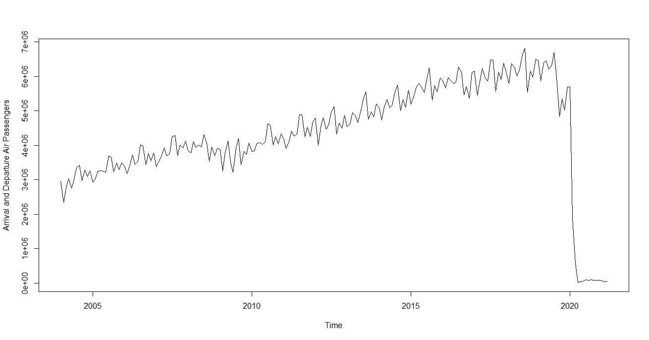
Refer to caption — Figure 1: Time Plot of Air Traffic Volume of Hong Kong International Airport

From the time plot 1 from January 2004 to December 2020, we can observe that the air traffic volume has obvious seasonal pattern³³3The seasonality of this time-series is discussed in detail in Section 4. and increases year by year although fluctuates monthly. Except for the normal observations of seasonality and non-stationarity, there are three subtle anomalies in the time plot.

•

Firstly, the volume of air traffic dropped a little bit in from early 2008 to 2009, since the financial crisis hit the prosperity of Hong Kong.
•

The most significant anomaly is that the air traffic dropped to around zero after 2020 due to the COVID-19 outbreak and air traffic control.
•

Before 2020, there is also a significant drop on the level of air traffic. I guess it is the series of political storms weaken people’s willingness to fly to Hong Kong. No matter the actual reason, it serves as another example of social data being significantly affected by a big event (or variable).

Considering these unpredictable major social changes, time-series model is imperfect since it focuses simply on the sequence itself, ignoring the other social variables. However, this gives the time-series model another applicable scenario, i.e., to quantifying 3 the effect of a major social change on a time-series. The operation is pretty simple. You just need to obtain the forecast of several periods $\{\hat{y}_{m+1},\hat{y}_{m+2},...,\hat{y}_{m+k}\}$ after the impact of major events, and the event influence can be obtained by subtracting the real value $\{y_{m+1},y_{m+2},...,y_{m+k}\}$ from the forecast value. Then, researchers can perform further study based on the difference sequence $\{\Delta_{m+1},\Delta_{m+2},...,\Delta\}$ .

The remaining parts of report are arranged as:

•

In Section 2, I discuss the modelling process for Hong Kong air traffic time-series. After model identification, model diagnosis, and model selection, sparse seasonal $\text{ARIMA}(0,1,1)\times(4,1,0)_{12}$ model is selected. The air traffic in the coming seven months locate precisely in the predicted $95\%$ confidence interval.
•

In Section 3, the sparse seasonal $\text{ARIMA}(0,1,1)\times(4,1,0)_{12}$ model is applied and fitted again to quantify the negative effect of COVID-19 on air traffic.
•

Finally, an analysis of seasonality and trend of this time-series is supplemented in Section 4.

2 Seasonal ARIMA Modelling

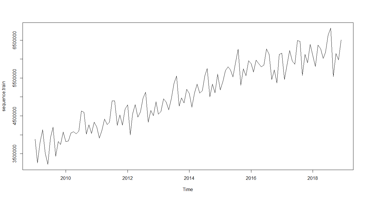
In this section, we use the data from (2009, 1) to (2018, 12) as train data, and the data from (2019, 1) to (2019, 7) as test sequence.

2.1 Discussion of Stationarity

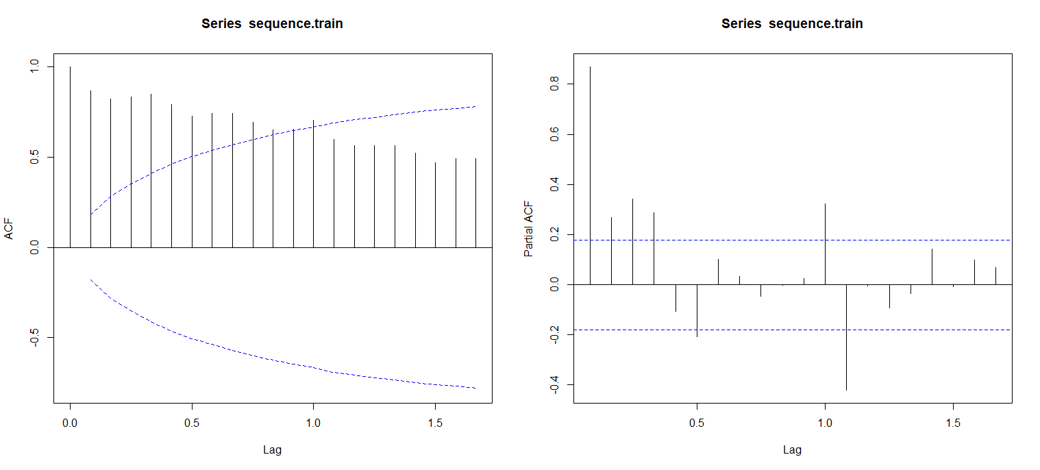
To get an initial understanding about the train sequence, we draw the time plot, sample auto-correlation function (ACF), and sample partial auto-correlation function (PACF) as Figure 2 and Figure 3.

We can observe from the time plot that the volume of air passengers went ups and downs in each year, but increases overtime. The sample ACF decays slowly from lag to lag, also indicating that the time-series is non-stationary. Another powerful tool to confirm the non-stationarity is performing the augmented dickey-fuller test (ADF test).

H_{0}:\text{The time-series is non stationary}\quad v.s.\quad H_{1}:\text{The time-series is stationary}

(1)

The test result is summarized in table 1.

Table 1: ADF tests for the original train sequence

Type 1			Type 2			Type 3
Lag	ADF	P.value	Lag	ADF	P.value	Lag	ADF	P.value
0	0.196	0.700	0	-2.309	0.208	0	-9.99	$\leqslant$ 0.01
1	0.753	0.859	1	-1.787	0.411	1	-7.75	$\leqslant$ 0.01
2	1.485	0.964	2	-1.162	0.640	2	-5.01	$\leqslant$ 0.01
3	2.237	0.990	3	-0.951	0.714	3	-3.36	0.0624
4	2.484	0.990	4	-0.955	0.712	4	-3.09	0.1191

Generally we consider only two types of ADF tests:

•

Type 1: , Assuming that the time-series has no drift and no trend.
•

Type 2: , Assuming that the time-series has drift but no trend.

Actually, the Type 3 ADF test assumes that the time-series has drift and trend. Since we are detecting the property of non-stationarity, we should not ignore the trend of the sequence. Thus, by looking at the first two types of ADF tests, the null hypothesis is not rejected consistently, which confirms the non-stationarity.

Considering the seasonal pattern and increase trend⁴⁴4See Section 4 for detailed analysis., we should take the differencing and seasonal differencing both⁵⁵5I tried to take the differencing only, the differenced sequence could pass the ADF tests but perform poorly in forecasting..

Now we can draw the time plot, sample ACF, and sample PACF of the differenced and seasonal differenced train sequence (dsd train sequence). Note that the sequence lost 13 observations after taking these two operations.

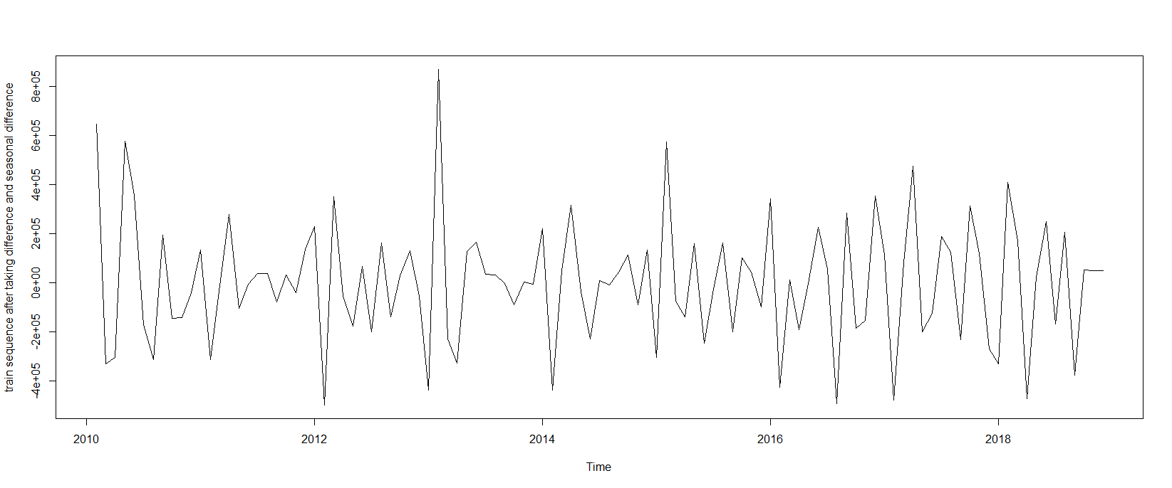
This time plot 4 seems contain no trend and fluctuates statioanrily. Then, I perform the ADF test again. The outcome of three types of ADF tests is shown in table 2, with null hypothesis rejected consistently. Note that the sequence after differencing twice will not contain drift, so we do not need to include drift in the model fitting step in the future.

Table 2: ADF tests for the dsd train sequence

Type 1			Type 2			Type 3
Lag	ADF	P.value	Lag	ADF	P.value	Lag	ADF	P.value
0	-19.26	$\leqslant$ 0.01	0	-19.20	$\leqslant$ 0.01	0	-19.14	$\leqslant$ 0.01
1	-19.17	$\leqslant$ 0.01	1	-19.12	$\leqslant$ 0.01	1	-19.06	$\leqslant$ 0.01
2	-13.00	$\leqslant$ 0.01	2	-12.97	$\leqslant$ 0.01	2	-12.93	$\leqslant$ 0.01
3	-9.17	$\leqslant$ 0.01	3	-9.15	$\leqslant$ 0.01	3	-9.12	$\leqslant$ 0.01
4	-7.41	$\leqslant$ 0.01	4	-7.39	$\leqslant$ 0.01	4	-7.36	$\leqslant$ 0.01

2.2 Model Identification

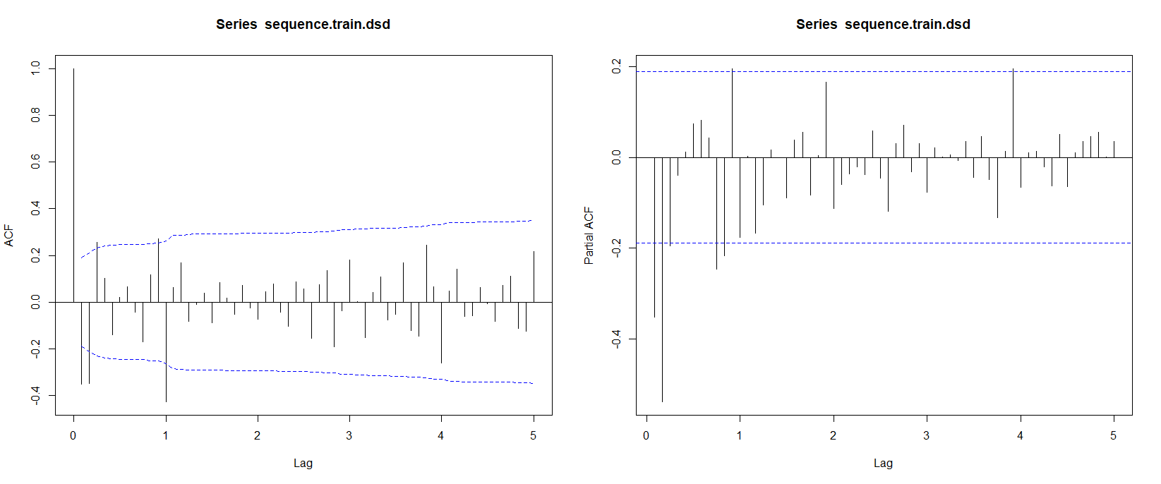
In this section, I will build a suitable seasonal ARIMA model by specifying the hyper-parameters $p,q,P,Q$ of $\text{ARIMA}(p,1,q)\times(P,1,Q)_{12}$ . The sample ACF and PACF plots are shown in Figure 5.

2.2.1 Identify Possible Models

From the first plot, lag-1, lag-2 are significantly outstanding, indicating that the MA part has $q=2$ . Lag-12 (seasonal lag-1) is even more outstanding and indicates $Q=1$ for SMA part.

As for the PACF plot, although it is generally considered to be treaky, I believe it can convey lots of useful information. As we can see, a clear spike appears at lag-1. And the partial auto-correlations around seasonal lag 1, 2, 4 locate at the boundary. This pattern of PACF at seasonal lags can not be ignored since it is weird and strong. I believe it is caused by SAR part, which might have hyper-parameter $1\leqslant P\leqslant 4$ . If $P\geqslant 1$ holds, the assumption of $Q=1$ for SMA part might not be true, since SAR will cause the auto-correlations at seasonal lags to decay slowly.

Since the situation is rather complex, I’d like to choose several pairs of possible hyper-parameters for my candidate models, and then fit and test them for adequacy. The four candidate models are summarized in table 3. My choice covers simple model like Model0 with $P=1$ and complex model like Model1 with $P=4$ . Since the correlations in the third seasonal lag of PACF plot is not significant, I also consider the Sparse Seasonal ARIMA (Model3), setting the parameter of SAR3 zero constantly. The reason why Model2 and Model3 are verified from Model1 while Model0 has no variations will be revealed later.

Model Name	Type	d	q	P	D	seasonal period
Model0	Seasonal ARIMA	1	2	1	1	12
Model1	Seasonal ARIMA	1	2	4	1	12
Model2	Seasonal ARIMA	1	1	4	1	12
Model3	Sparse Seasonal ARIMA	1	1	4(3)	1	12

Table 3: Four candidate models

2.2.2 Parameter Estimation for Candidate Models

The maximum likelihood estimation of the parameters and their corresponding standard errors are provided in table 4 and table 5.

Table 4: Fitted Model0 and Model1

	Model0			Model1
	ma1	ma2	sar1	ma1	ma2	sar1	sar2	sar3	sar4
coefficient	-0.6772	-0.1322	-0.5195	-0.6072	-0.1427	-0.7524	-0.5570	-0.2826	-0.4239
standard error	0.1359	0.1547	0.0914	0.1065	0.1208	0.1044	0.1447	0.1465	0.1099
	AIC	2901.09			AIC	2876.77	BIC	2895.48

Table 5: Fitted Model2 and Model3

	Model2					Model3
	ma1	sar1	sar2	sar3	sar4	ma1	sar1	sar2	sar4
coefficient	-0.6877	-0.7372	-0.5510	-0.2600	-0.4179	-0.6960	-0.6535	-0.3670	-0.2897
standard error	0.0891	0.1066	0.1473	0.1464	0.1123	0.0827	0.0991	0.1032	0.0940
	AIC	2876.13	BIC	2892.17		AIC	2877.09	BIC	2890.46

From the first MLE table 4, we can find that the coefficients of ma2 in both Model0 and Model1 are insignificant. Also, the coefficient of sar3 is insignificant.

Model2 in table 5 deletes the ma2, but the coefficient of sar3 is still insignificant. Sparse Model3 set the coefficient of sar3 to zero and its remaining coefficients are all significant. Consequently, the Sparse Model3 seems to be a satisfying variation from Model1 up to now.

Note that the reason why I haven’t fit a $\text{ARIMA}(0,1,1)\times(1,1,0)_{12}$ model here is that Model0 itself is inadequate. With an inadequate model, it’s unwise to make it even simpler, so I will use Model3 for further exploration. For the sack of illustration, I will also show the testing results of Model0 in the following section.

2.3 Model Diagnosis

2.3.1 Residual Analysis of Candidate Models

Residual analysis will be performed to check the residual normality and model adequacy.

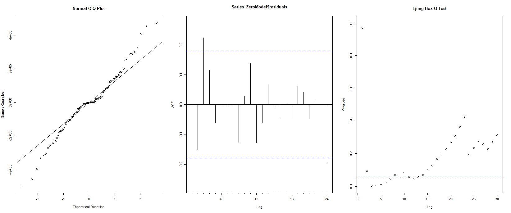
The Ljung-box test in Figure 6 for Model0 shows that many test statistics at different lags have value less than the threshold 0.05. Whats more, the Shapiro-Wilk normality test reject the normal hypothesis with a p-value of 0.01871.

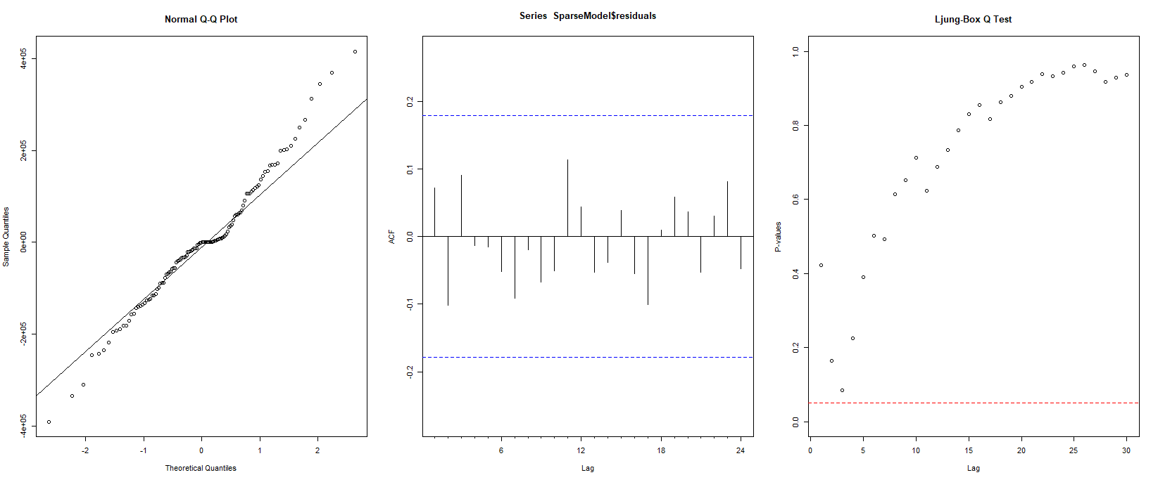
As for the Model3, in Figure 7, the residuals locate near the 45 degree line and the p-value of Shapiro-Wilk Normality Test is 0.1006, p-value of Jarque Bera Test is 0.1683, both greater than 0.05. Combining tests and observation, we don’t reject the normal hypothesis. On the other hand, the Ljung-box test and the ACF show that there is no other correlation pattern left in the residuals, thus Model3 is adequate and promising enough.

2.3.2 Analysis of Over-Parameterized Models

To check the stability of Model3, we will fit some over-parameterized models for comparison. Since increasing the order of MA reaches to Model2, which has insignificant coefficient of ma2. Increasing the order of AR brings calculation problem for likelihood, making MLE, AIC, AICc, and BIC incalculable. So here we just consider two cases of over-parametrized models ⁶⁶6Both are sparse models with sar3=0.:

\text{OverSAR}:\text{ARIMA}(0,1,1)\times(5,1,0)_{12}\quad\text{OverSMA}:\text{ARIMA}(0,1,1)\times(4,1,1)_{12}

The MLE of OverSAR and OverSAR are summarized in table 6.

Table 6: MLE of over-parameterized models

	OverSAR					OverSMA
	ma1	sar1	sar2	sar4	sar5	ma1	sar1	sar2	sar4	sma1
coef.	-0.6962	-0.6619	-0.3618	-0.3062	-0.0323	-0.6997	-0.3387	-0.2191	-0.3847	-0.4654
s.e.	0.0821	0.1031	0.1037	0.1117	0.1197	0.0824	0.1590	0.1362	0.1051	0.2119
	AIC	2879.02	BIC	2895.06		AIC	2876.2	BIC	2892.24

The sar5 for OverSAR is insignificant, so Model3 is stable. The sma1 for OverSMA can be regarded as significant while its sar2 becomes insignificant. So we may fit and test the adequacy of another model. $\text{Model4}:\text{ARIMA}(0,1,1)\times(4,1,1)_{12}$ with sar2=0 and sar3=0. The MLE result in table 7 shows that the coefficient of sar1 is insignificant, then I also fit the $\text{Model5}:\text{ARIMA}(0,1,1)\times(4,1,1)_{12}$ with sar1 = sar2 = sar3 = 0, whose coefficients are all significant.

Table 7: MLE of Model4 and Model5

	OverSAR				OverSMA
	ma1	sar1	sar4	sma1	ma1	sar4	sma1
coef.	-0.7148	-0.2018	-0.3949	-0.6534	-0.7251	-0.3631	-0.8222
s.e.	0.0782	0.1190	0.1133	0.1571	0.0761	0.1236	0.1667
	AIC	2876.52	BIC	2889.89	AIC	2877.18	BIC	2887.87

Then I carried out the Ljung-box test for Model5, the result shows that this model is not so adequate as Model3. Considering the AIC and BIC of these two models are rather similar, I choose Model3 as my final model.

2.4 Forecasting

2.4.1 Forecast 7 periods

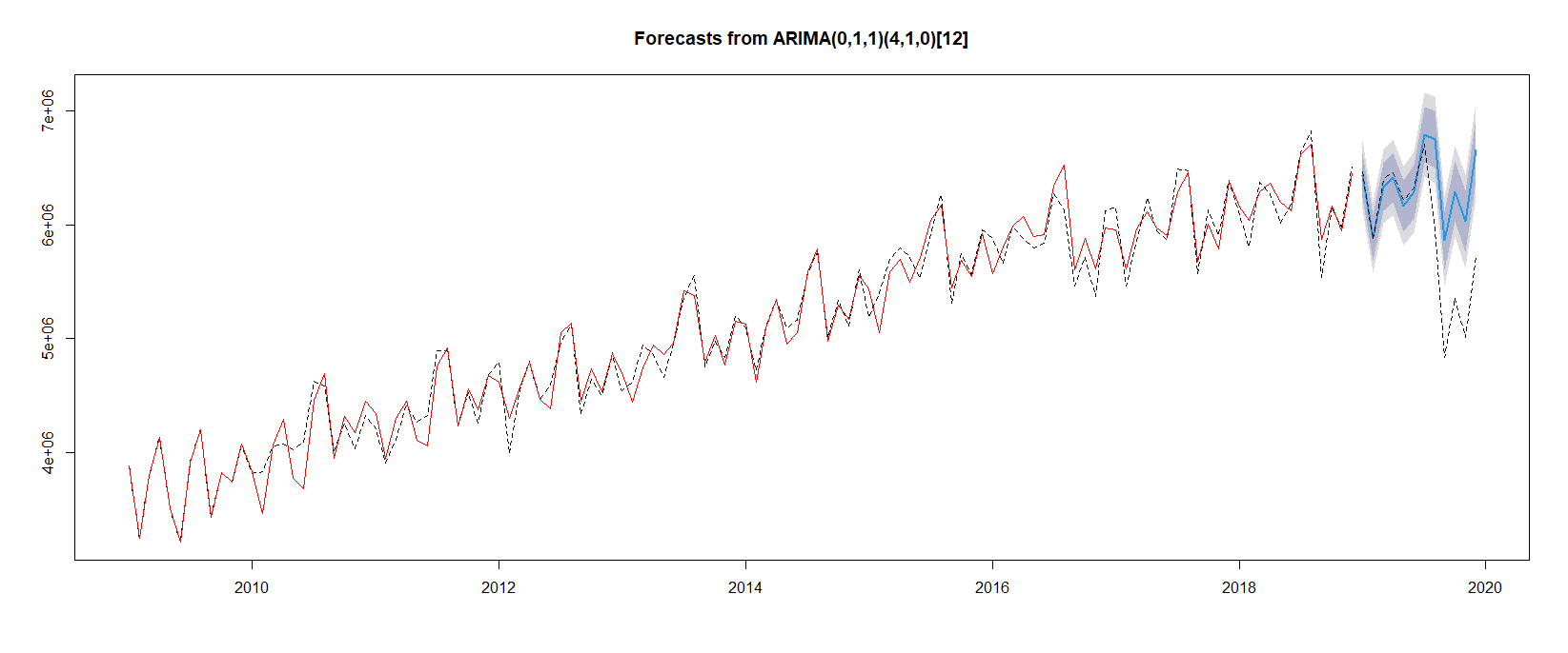
With my final model, I forecast the air traffic of Hong Kong International Airport from January 2019 to July 2019. All the true value fall in the 95 $\%$ confidence interval⁷⁷7The red line indicates the fitted value of train sequence. The black dotted line indicates the true value. The blue line is the predicted sequence, the shallow shadowed area is the 80 $\%$ C.I. and the heavy shadowed area is the 95 $\%$ C.I... The selected model functions well in predicting air traffic when the social environment is rather stable.

For the convenience of reading, I also put down the number in table 11.

Month	Turth	Predicted	95 Lower	95 Upper	80 Lower	80 Upper
Jan	6460193	6431575	6238776	6624374	6136715	6726436
Feb	5866706	5884746	5683235	6086257	5576561	6192930
Mar	6396906	6331132	6121270	6540993	6010176	6652088
Apr	6464336	6413993	6196101	6631886	6080755	6747232
May	6209935	6164378	5938740	6390016	5819295	6509462
Jun	6319690	6285538	6052412	6518664	5929003	6642074
Jul	6702076	6787117	6546736	7027498	6419486	7154748

Table 8: Ground truth, predicted value, and confidence intervals

2.4.2 Forecast Precision Comparison

I tried to calculate the Mean Squared Error of Model0, Model1, Model2, Model3, OverSAR, OverSMA, Model4, and Model5 mentioned before. Actually, our final choice——Model3 outperforms other models on this metric also.

This also testify that the previous decision of choosing Model3 rather than Model5, regarding Model5 is less adequate, is correct.

Model0	Model1	Model2	Model3	OverSAR	OverSMA	Model4	Model5
64532.64	52624.96	52483.63	51379.15	53735.19	57491.59	60974.08	61514.54

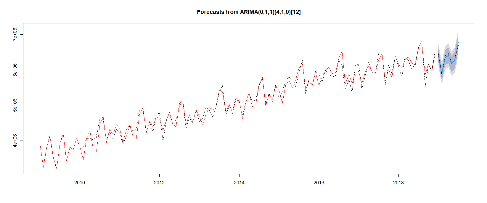
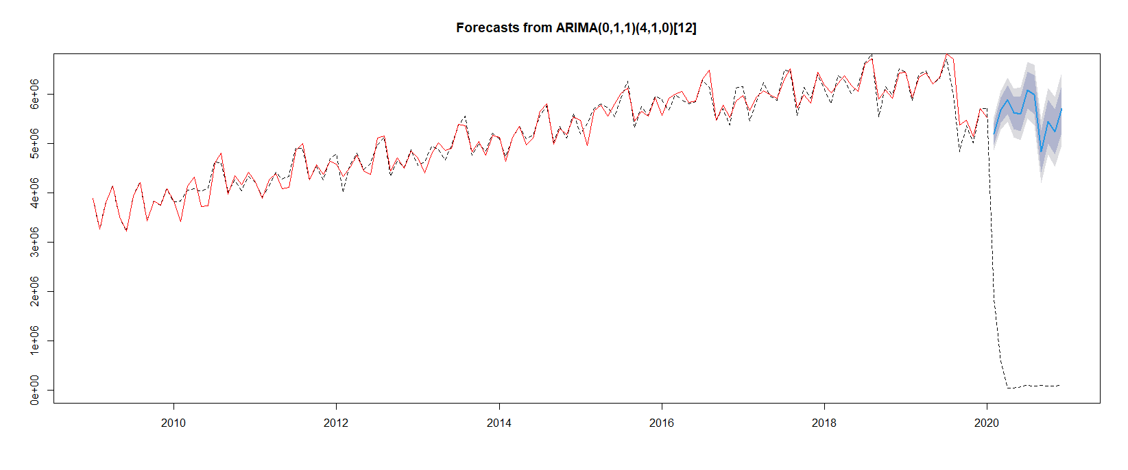
Table 9: MSE comparison between all models fitted before

2.4.3 What will happen if we forecast 12 periods

In the previous forecasting, the social environment is mainly stable. From June 2020, political storm is coming, the arrival and departure air passengers are both affected greatly by the unstable social situation. If we use the selected sparse seasonal ARIMA model to predict the air traffic from August 2020 to December 2020, as shown in Figure 9, the predicted value seem to be parallel with the true value but over estimated by a large margin.

Obviously, the time-series model cannot adjust itself when a major social event happened. The model will predict as if the society is developing as usual. This bring us an insight that we can use the time-series model fitted before some event happened to estimate the margin or effect caused by that event.

3 Quantify the Effect of Pandemic

In this section, we fit the Model3 with data from (2009,1) to (2021,1), kicking out the effect of political storm. Then, we’ll use it to predict the air traffic value of the remaining eleven months in 2020.

3.0.1 Refitting the Final Model

The MLE of our model on new data is summarized in table 10.

Table 10: Fitted Model2 and Model3

	ma1	sar1	sar2	sar3	sar4
coefficient	-0.3925	-0.6385	-0.4025	0	-0.2848
standard error	0.0924	0.0975	0.0941	0	0.0895
	AIC	3257.33	BIC	3271.27

3.0.2 Forecast and Quantification of Loss

I take the difference between predicted value and true value as predicted loss. The rate shows that COVID-19 made loss of 95 $\%$ of air passengers in the late eleven months of 2020. And the most severe month was April, with a lost of $99.95\%$ air traffic as it should have without COVID-19.

Month	Turth	Predicted	Predicted Loss	1-Loss rate
Feb	1877718	5191726	5683235	0.361675
Mar	575825	5673103	6121270	0.10150
Apr	31739	5883236	6196101	0.00539
May	37423	5616262	5938740	0.00666
Jun	59199	5597481	6052412	0.01058
Jul	96028	6077110	6546736	0.01580
Aug	83807	5986478	6238776	0.01400
Sep	99805	4833198	5938740	0.02065
Oct	79360	5442955	6052412	0.01458
Nov	81001	5234962	6546736	0.01547
Dec	90531	5701242	6238776	0.01588
Overall	3112436	61237753	58125317	5.08 $\%$

Table 11: Estimation of the loss of air traffic due to COVID-19

4 Decomposition for Explanation

The air traffic time-series can be decomposed into three parts: trend, seasonal pattern, and random noise. Ignoring the random noise, we can plot the trend and seasonal pattern as Figure 11.

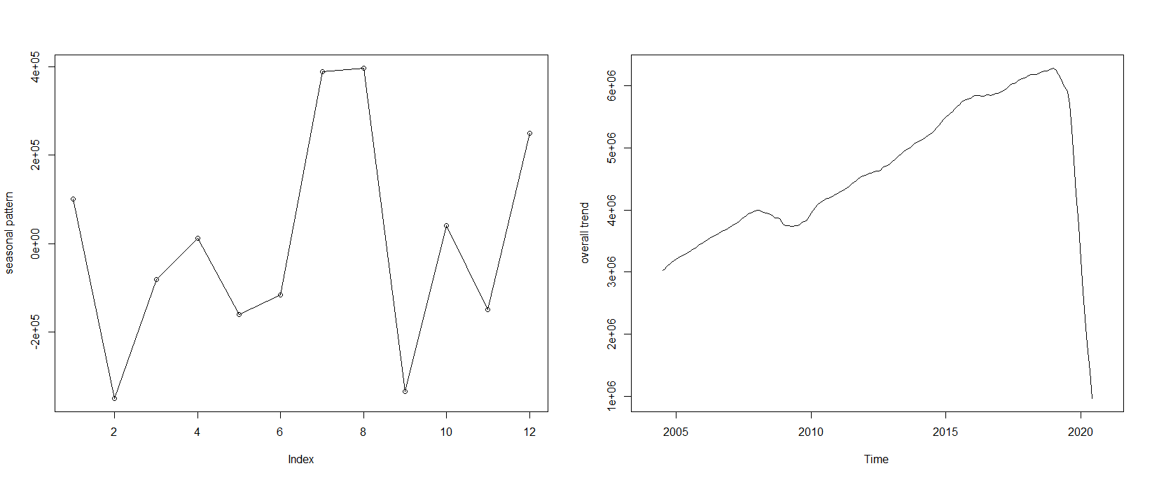
4.1 Analysis of the Trend

The level of air traffic increased as the economy developed from 2004 to 2019, except for a small drop back in 2008.

4.2 Analysis of the Seasonal Pattern

Generally, August and July are the peak season, following by December and January. The underlying reason might be simple: The tourism in Hong Kong is prosperous in summer, and students also flow frequently in these months. As for the winter peak, it might be partly due to the spring festival, when lots of people working or studying in Hong Kong fly back to their home city or just go for a trip.

5 Conclusion

Sparse Seasonal ARIMA Model3 does a great job in predicting future air traffic of Hong Kong International Airport in a stable social environment. Although it fails to react to the social change automatically, it can still be used to evaluate the effect of social change on the air traffic time-series. I believe it can be extended to other topics of economic and social statistics.