DiagViB-6: A Diagnostic Benchmark Suite for Vision Models in the Presence of Shortcut and Generalization Opportunities

Abstract

Common deep neural networks (DNNs) for image classification have been shown to rely on shortcut opportunities (SO) in the form of predictive and easy-to-represent visual factors. This is known as shortcut learning and leads to impaired generalization. In this work, we show that common DNNs also suffer from shortcut learning when predicting only basic visual object factors of variation (FoV) such as shape, color, or texture. We argue that besides shortcut opportunities, generalization opportunities (GO) are also an inherent part of real-world vision data and arise from partial independence between predicted classes and FoVs. We also argue that it is necessary for DNNs to exploit GO to overcome shortcut learning. Our core contribution is to introduce the Diagnostic Vision Benchmark suite DiagViB-6, which includes datasets and metrics to study a network’s shortcut vulnerability and generalization capability for six independent FoV. In particular, DiagViB-6 allows controlling the type and degree of SO and GO in a dataset. We benchmark a wide range of popular vision architectures and show that they can exploit GO only to a limited extent.

1 Introduction

Despite their state-of-the-art performance on object classification tasks, deep neural networks (DNN) are highly prone to shortcut learning [8, 33, 11]. Instead of learning holistic representations and decision rules that can generalize beyond the training data, DNNs overly rely on so-called shortcut opportunities (SO), which occur when the target class is highly correlated to one or very few easy-to-represent input factors [12]. This leads to poor generalization on many out-of-distribution (OOD) settings, e.g. ImageNet trained DNNs are biased towards texture and fail to generalize under texture-shape cue conflict evaluation [8].

Figure 1: Exemplar study in our proposed benchmark. The network is trained to predict factor classes 2, 4, 3 for the shape factor with varying hue. All five depicted training combinations are uniformly shown during training. The shape 2 co-occurs solely with the blue class of the hue factor, which poses a shortcut opportunity. The shapes 4 and 3 occur uniformly with hue red and green; these combinations pose a generalization opportunity, since they reduce the predictiveness of the hue factor for the shape factor. Test accuracy is computed on examples from OOD factor combinations to evaluate a model’s shortcut vulnerability in the context of the given generalization opportunity.

While humans are also prone to shortcut learning in certain cases, such as object classification under context-based cue conflict settings [29], the biological model remains largely unaffected by shortcuts when it comes to predicting basic object factors of variation (FoV) such as shape, hue or texture. This “shortcut-immunity” w.r.t. basic FoV is just as necessary for intelligent systems; thus, efforts towards improving model generalization are of utmost importance.

Existing literature studies shortcut behavior in DNNs mainly in the context of object classification. In this work, we address a more fundamental variant of shortcut learning, focusing specifically on the prediction of basic FoV themselves, similar to [12]. In the context of FoV prediction, we refer to different manifestations of a factor as factor classes. For example, “red” and “green” are factor classes for the factor hue, whereas “circle” and “elephant shape” are factor classes for the factor shape. Object classes such as “elephant” or “car” are characterized by the co-occurrence of certain factor classes, e.g. “gray”, “elephant shape”, and “elephant texture” characterize an elephant. SO arise from this co-occurrence of different factor classes.

As stated in [7], SO are a property of real-world vision data. In this work, we propose to additionally consider generalization opportunities (GO), which are a relaxation of the strict correlation (or co-occurrence) between a target class and an input FoV at training time. For instance, consider the object “car” with factors shape and color; cars appearing in different colors during training would induce a GO compared to cars appearing only in one color. We refer to such cases as compositional-based GO. Correlations can also be violated in the form of outliers consisting of rare combinations of factor classes, e.g. a “white elephant”. We refer to these cases as frequency-based GO.

A straightforward approach to introduce GO in the training data is data augmentation. For example, [21] applies random color transformations to the training images, removing a potential correlation between the target class and the factor color. However, data augmentation results in models that are invariant with respect to the augmented factor. Such models lose important information that may be needed to properly identify and reason about OOD samples. In contrast to being invariant, we argue that a good vision model needs to have an explicit representation of these FoV. Our work aims at analyzing a model’s capability to exploit the GO already present in the data, as opposed to adding more GO to a dataset, as done in data augmentation. While several synthetic benchmark datasets for compositional generalization and cue-conflict settings already exist [12, 2, 28], none of them enables sufficient and systematic control over the SO and GO present in the dataset for a broad set of different visual object FoV.

Inspired by prior work on shortcut learning and compositional generalization [7, 12], we present a synthetic but diagnostic benchmark suite DiagViB-6 that includes different studies to evaluate a model’s shortcut vulnerability under varying degrees of GO. Figure 1 illustrates an exemplar study in our benchmark. The benchmark suite contains an image-generating function that allows direct and independent control over the six basic, visual object FoV: position, hue, lightness, scale, shape, and texture (Fig. 2). Additionally, our framework provides a dataset-generating function that enables a user to control the nature of SO and GO appearing in a dataset. This is achieved by introducing different degrees of correlation between factors, and inducing co-occurrences of certain factor class combinations. Furthermore, the benchmark suite provides metrics to evaluate a model’s shortcut vulnerability under different GO for each factor.

We evaluate a wide range of common deep learning vision models on our benchmark and perform an exhaustive investigation of their shortcut vulnerability w.r.t. the six stated FoV. We show that while they exploit frequency GO, they exploit the more relevant compositional GO only to a limited extent. This holds true also for approaches specifically designed to counteract shortcut learning.

We admit that this benchmark suite does not sufficiently and directly prove a vision model’s ability to generalize on real-world data (e.g. object classification on ImageNet). However, it serves as a critical diagnosis that is necessary in order to study a model’s shortcut vulnerability and generalization ability under various controlled tasks and data setups. Ultimately, the design of our benchmark suite allows a user to control different degrees of SO and GO in a dataset (not commonly available in real-world data), in order to assess a model’s behavior under different conditions.

Our contributions in this work can be summarized as follows: We propose a benchmark suite to create datasets that enable the user to independently combine six visual FoV, allowing explicit control over which SO and GO are present in the resulting data. We establish suitable metrics to evaluate both a model’s shortcut vulnerability, and its capability to exploit GO in the data. Lastly, we provide empirical evidence that common vision architectures exploit GO only to a limited extent, especially compositional-based GO.

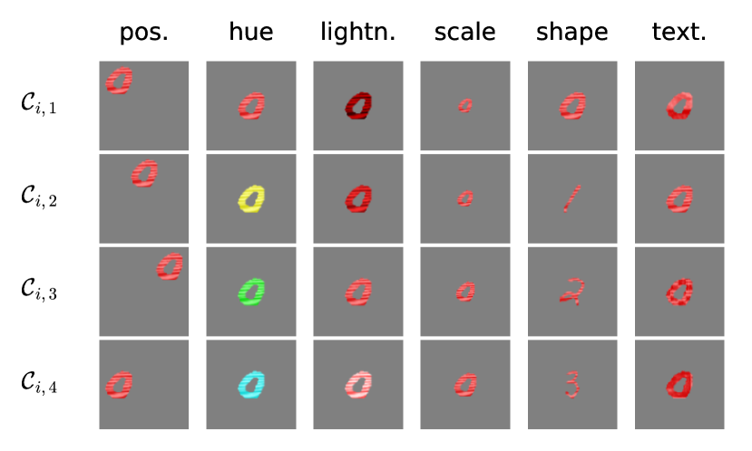
Figure 2: Image space traversal across all six FoV and four corresponding class labels used in this work. Along each column only the corresponding factor is varied, while all others are fixed. Note that some factors have more than the four classes shown here (refer Tab. 1).

2 Related work

Compositional generalization in visual attribute prediction

Our work is formulated under the general framework of visual attribute prediction. In contrast to classical object recognition, the task is to learn semantic attributes of a given object [6, 32]. By learning such class-agnostic visual object attributes, models can make useful predictions about object classes that have not been seen at training time. We are interested in specific scenarios, called compositional generalization, in which only a limited number of attribute combinations are provided during training. The model needs to generalize during training in order to handle inputs with unseen attribute combinations during testing [27, 28, 35, 24, 1, 2, 36]. While most of these works use a multi-task setup requiring object and attribute annotations for every image during training, we consider a single-task prediction, in which only one factor is predicted. In addition, we consider predicting more fundamental factors (e.g. lightness, scale, hue) that are independent of each other and can be applied to all types of objects, as opposed to high-level visual attributes (e.g. glossy, furry, smooth).

Shortcut learning

In recent years, multiple works have shown that DNNs are vulnerable to shortcut learning on several real-world and synthetic datasets [3, 8, 11, 7, 12]. As a result, many studies investigate the reasons for shortcut learning, and propose methods to alleviate such vulnerabilities. It is suggested in [11] that differences between humans and DNNs may arise from differences in the data that they see. [12] investigated how a model’s representations are shaped by inductive biases in the presence of SO. A common attempt to overcome shortcut learning is to augment the training data with handcrafted transformations in order to reduce the importance of each individual factor (e.g. shape or texture) [8, 23]. This approach has further been extended to generative model-based augmentations [31, 34, 33]. Recently, [26] showed that for self-supervised learning, certain shortcut features can be removed automatically, under the assumption that such features are most vulnerable to adversarial attacks. Most of the aforementioned works on shortcut learning are benchmarked on black-box datasets (e.g. Stylized ImageNet [8]), leading to a limited, implicit knowledge of the SO and GO introduced in both the training and test data. In contrast, our DiagViB-6 enables explicit image generation, allowing shortcuts learned from individual FoV to be evaluated.

Benchmarks

Numerous works exist on related areas, such as compositional generalization or disentanglement of FoV, that introduce datasets which allow to control image factors to some extent [12, 16, 2, 17, 20, 3, 13, 22, 15, 36]. However, these all contain shortcomings that we try to address in our work.

In contrast to [12, 2, 17, 20, 3, 13], our dataset contains a richer intra-factor class variation. E.g. for the shape factor, each digit class of MNIST specifies a factor class. During image generation we use different instances of each individual factor class. Similarly, for red, we use different tones of red. Other datasets only provide for example a single cylinder shape or red tone. For an overview of the variation provided for each of our six factors see Sec. A.1.

Unlike the datasets in [12, 20, 3, 22], which use only 2-3 FoV, DiagViB-6 includes six fundamental FoV that all good vision models should be shortcut-robust towards.

Some works, e.g. [12], investigate the internal feature representations of DNNs at certain layers, whereas our benchmark depends only on a model’s predictions and is therefore architecture agnostic.

In contrast to multi-attribute prediction [2, 15, 36], we evaluate a model’s shortcut behavior w.r.t. a single factor under different correlations to other FoV. This allows for a more structured and comprehensive analysis of shortcut behavior, where the interaction between individual factors can be investigated.

3 Diagnostic vision benchmark suite

This section describes our benchmark suite DiagViB-6, used to examine the shortcut vulnerability and generalization capability of DNNs over six different independent FoV. The suite consists of different image datasets tailored for different diagnostic studies, as well as suitable metrics for measuring shortcut vulnerability. We begin with an overview of the image generation process in our benchmark studies (Sec. 3.1), describe the benchmark setup in Sec. 3.2, introduce different studies in Sec. 3.3, and lastly establish the metrics to evaluate DNNs on our studies in Sec. 3.4.

3.1 Prerequisite

$\mathcal{F}_{i}$	$\mathcal{S}_{i}$	$\mathcal{N}_{i}$	$\mathcal{C}_{i,1}$	$\mathcal{S}_{i,1}$
position	$[0,1]^{2}$	9	top-left	$[0.1,0.3]\times[0.1,0.3]$
hue	$[0,2\pi)$	6	red	$[$$,$$]$
lightness	$[0,1]^{2}$	4	dark	$[0,0.1]\times[0.4,0.5]$
scale	$[0.69,1.45]$	5	small	$[0.69,0.74]$
shape	MNIST	10	‘0’	digits ‘0’
texture	textures	5	tiles	tiles texture crops

Table 1: Overview of factors $\mathcal{F}_{i}$, respective factor spaces $\mathcal{S}_{i}$, and number of classes $\mathcal{N}_{i}$. $\mathcal{C}_{i,1}$ & $\mathcal{S}_{i,1}$ are exemplary factor classes and factor space regions of class label 1.

Fundamentals

Datasets in our benchmark suite consist of images with a single object described by a fixed, pre-defined set of six independent factors. Each factor $\mathcal{F}_{i},\,i\in\{1,\ldots,6\}$ corresponds to a semantically meaningful image attribute: shape, texture, hue, lightness, position and scale. Every factor $\mathcal{F}_{i}$ is associated with a certain factor space $\mathcal{S}_{i}$ from which factor realizations $f_{i}{\color[rgb]{0,0,0}\widehat{=}f_{\mathcal{F}_{i}}}\in\mathcal{S}_{i}$ that describe the objects are sampled. For example, lightness of an object $f_{\text{lightness}}$ can be realized as a scalar sampled from $\mathcal{S}_{\text{lightness}}=[0,1]$. We assign $\mathcal{N}_{i}$ discrete factor class labels for each factor, denoted as $\mathcal{C}_{i,j}$, $j\in\{1,\ldots,\mathcal{N}_{i}\}$, which correspond to regions $\mathcal{S}_{i,j}\subset\mathcal{S}_{i}~{}\forall j$ and $\mathcal{S}_{i,j}\cap\mathcal{S}_{i,k}=\emptyset,j\neq k$. Similar to factors, each factor class $\mathcal{C}_{i,j}$ corresponds to a semantically meaningful attribute class (e.g. $\mathcal{C}_{\text{lightness},1}$ refers to “dark” and $\mathcal{C}_{\text{hue},3}$ refers to “green”). Note that our choice of classes for each factor is arbitrary and based on human intuition (similar to [12]) and thus our work does not evaluate a factor’s general ability to act as a shortcut over another.

Table 1 provides an overview of the list of factors, their corresponding factor spaces, and the number of factor classes used throughout this work. As examples, the factor spaces $\mathcal{S}_{i,1}$ and the factor classes $\mathcal{C}_{i,1}$ are also provided. A comprehensive overview of factor spaces for all factor classes is provided in Sec. A.1.

Image generation

An image is generated by defining a combination of factor classes $\mathcal{C}\,=\,(\mathcal{C}_{1,j},\mathcal{C}_{2,k},\ldots,\mathcal{C}_{6,l})$, one from each factor $\mathcal{F}_{i}$. This is done by first sampling factor realizations $f_{i}$ from the corresponding regions ($\mathcal{S}_{1,j},\mathcal{S}_{2,k},...,\mathcal{S}_{6,l}$) and then generating unique images from those sampled $f_{i}$ using an image-generating function $I:(f_{1},f_{2}...,f_{6})\rightarrow\mathcal{I}$ with $\mathcal{I}\in[0,1]^{H\times W\times 3}$, where $H=W=128$. The six FoV are incorporated into the image as follows: $f_{\text{shape}}$ is always an instance of a digit in the MNIST dataset, which is then thresholded to yield a binary segmentation. From the two lightness values $f_{\text{lightness}}=(f_{\text{lightness}}^{(1)},f_{\text{lightness}}^{(2)})$ two colors with equal hue $f_{\text{hue}}$ are generated. The $f_{\text{texture}}$’s are crops of histogram-normalized grey-scale texture images and their pixel values serve as the coefficients of a convex combination between the two aforementioned colors, resulting in the final color. The object is then either up or down-sampled depending on the chosen scale realization $f_{\text{scale}}$, and placed at a specific position $f_{\text{position}}$ on a greyscale background.

Figure 2 illustrates the variation over the six different FoV. In particular, the first column is generated with factor class labels $\mathcal{C}=(\mathcal{C}_{pos.,j},\,\mathcal{C}_{hue,1},\,\mathcal{C}_{lightn.,3},\,\mathcal{C}_{scale,5},\\ \mathcal{C}_{shape,1},\mathcal{C}_{text.,2})$ with $j\in\{1,\,2,\,3,\,4\}$. Similarly, the other columns show images varying one factor while keeping the classes of all other factors fixed. Note that the six different FoV are independent, and thus different images can be generated for each of the $\prod_{i}\mathcal{N}_{i}=54000$ different factor class combinations.

3.2 Benchmark Setup

In this section we lay out the fundamentals used in Sec. 3.3 to design and conduct studies analyzing different aspects of a DNN’s shortcut behavior.

For all studies, we select a subset of three factor classes from the $\mathcal{N}_{i}$ available for each factor $\mathcal{F}_{i}$, which are then used during training, validation and testing. For example, as depicted in Fig. 1 and 3, we select the factor classes $\{\text{Blue},\text{Red},\text{Green}\}$ and $\{\texttt{2},\,\texttt{4},\,\texttt{3}\}$ for factors $\mathcal{F}_{hue}$ and $\mathcal{F}_{shape}$, respectively, and similarly for the other factors. This results in $3^{6}=729$ different factor class combinations out of the mentioned $54000$ being used for a single experiment. Choosing the same number of factor classes across factors simplifies evaluation and removes the number of factor classes as a source of variation. To account for randomness introduced by this selection of factor classes, we draw five random dataset samples of selected factor classes, over which reported results are averaged.

As mentioned in Sec. 1, we want to evaluate a network’s shortcut behavior when predicting an FoV in the presence of varying amounts of SO and GO in the training data. In this work, we consider the interplay between all possible pairings of two factors $(\mathcal{F}_{i},\mathcal{F}_{j})$. For each pairing, the task is to predict the class of the first factor $\mathcal{F}_{i}$, where SO and GO are induced by a specified co-occurrence pattern of factor class combinations for $\mathcal{F}_{i}$ and $\mathcal{F}_{j}$. For example, consider the setup in Fig. 1, with $\mathcal{F}_{i}$: shape and $\mathcal{F}_{j}$: hue. Only five out of the nine possible combinations of factor classes (dashed rectangles in Fig. 1) are shown during training, which induces a shortcut opportunity for the blue “$2$”. During testing, we then evaluate the networks performance on the OOD combinations (solid rectangles in Fig. 1). The other $4$ factors are not correlated with $\mathcal{F}_{i}$ or $\mathcal{F}_{j}$; their factor classes all appear with the same uniform probability. We conduct an exhaustive analysis of all possible factor pairings, resulting in $6\times(6-1)=30$ different settings, i.e. $6-1$ possible pairings for each target factor.

We generate validation data following the same distribution as the training data. In contrast, test data is designed to analyze a model’s shortcut behaviour by violating the pairwise correlations existing in the training data, and thus contain OOD samples in the $3\times 3$ matrix (cf. $\times$ for training and $\bigcirc$ for testing in Fig. 3). We always generate $43\,740$ training, $8748$ validation, and $10\,000$ test samples.

Figure 3: Schematic overview of conducted studies (cf. Fig. 1). For a combination of two factors $\mathcal{F}_{i},\mathcal{F}_{j}$ ($x$- and $y$-axis), we select three factor classes (rows and columns) for each factor and predict the first ($y$-axis) factor. Different selections from the resulting nine combinations of factor classes for training and test datasets ($\times$ and $\bigcirc$) yield different GO and SO settings: The zero SO (ZSO), the three degrees of frequency GO (FGO) (increasing size of crosses $\times$ , $\times$ , $\times$ indicate increasing OOD frequency during training), the zero GO (ZGO), the three compositional GO (CGO-1/2/3) settings and the compositional hybrid GO (CHGO).

3.3 Benchmark Studies

Having introduced the general structure of our benchmark, we now provide an overview of the five studies it enables (see Fig. 3 for illustration).

Zero Shortcut Opportunities (ZSO)

The goal of this first study is to measure a network’s factor classification performance in the absence of any SO. In the ZSO training data, each class of the target factor $\mathcal{F}_{i}$ co-occurs uniformly with all possible classes of $\mathcal{F}_{j}$, as indicated by the positions of $\times$s in the top-right of Fig. 3. Thus, $\mathcal{F}_{j}$ is not predictive for $\mathcal{F}_{i},~{}\forall i\neq j$. After training, the factor-classification performance of the model is tested on a dataset that shares the same distribution as the training data (see $\bigcirc$ in Fig. 3).

Zero Generalization Opportunities (ZGO)

This study can be considered an “opposite” of the ZSO study. In the ZGO training data, the target FoV $\mathcal{F}_{i}$ is perfectly correlated with $\mathcal{F}_{j}$, i.e. each class of $\mathcal{F}_{i}$ can only co-occur exclusively with one particular class of $\mathcal{F}_{j}$ (see ZGO in Fig. 3). Since both factors contain redundant information for the prediction task, $\mathcal{F}_{j}$ can be exploited as a shortcut to predict $\mathcal{F}_{i}$.

Compositional Generalization Opportunities (CGO)

With the ZSO and ZGO studies capturing the two extremes, we continue with more realistic setups where both SO and GO are present in the training data. As mentioned in Sec. 1, one way to introduce GO is through compositions. The CGO study does exactly this, addressing compositional GO by successively adding more factor class combinations for $\mathcal{F}_{i},~{}\mathcal{F}_{j}$ into the training set. In particular, we generate three sub-studies CGO-$c,~{}c\in\{1,2,3\}$ with increasing degree of GO (Fig. 3); the added combination is picked at random. For each class of the target factor, we hold out at least one unseen combination for testing, as indicated by the $\bigcirc$ symbols in each row in the CGO-$c$ diagrams of Fig. 3. For $c=0$, no GO are provided and thus CGO-0 is identical to the ZGO study discussed above. The goal of the CGO studies is to quantify a model’s generalization capability, i.e. the capability to efficiently exploit the GO present in the data. We would expect a good vision model to perform well on these generalization tasks, especially as the number of SO decreases and the number of GO increases.

Compositional Hybrid GO (CHGO)

This is a special case of CGO-2, for which both SO and GO are present, but explicitly separated, as depicted in Fig. 3 (bottom-left). One can think of this as a mixture of ZSO and ZGO, in which one of the classes of $\mathcal{F}_{i}$ is exclusively coupled with a certain class of $\mathcal{F}_{j}$ (ZGO), while the remaining two target factor classes co-occur uniformly with the remaining two classes of $\mathcal{F}_{j}$ (ZSO). The goal of CHGO is to examine whether a model can become immune to an extreme SO by exploiting GO available for other classes of the same factors.

As pointed out in Sec. 1, this heterogeneous mixture of SO and GO comes closest to real-world data. For instance, school buses might always be “yellow” while other cars appear in arbitrary colors besides yellow. Considering a model that predicts object shape, the yellow buses allow the model to shortcut its bus-shape prediction by solely relying on object color. A good vision model should now be able to exploit the provided GO, in the form of differently colored cars, to also predict the correct shape for an OOD “red” bus.

Frequency-based Generalization Opportunities (FGO)

Orthogonal to the CGO study, GO may also be introduced in a frequency-based manner i.e., controlling the proportion of a correlation introduced in the training data (cf. [12, 4]). These sub-studies can also be seen as a transition from ZGO to ZSO by gradually increasing the frequency of correlations in the training data. We generate three sub-studies FGO-$f,~{}f=\{5,\,10,\,20\}$, where the strict correlation from the ZGO is relaxed by means of low frequency violations (in $f\,$\mathrm{\char 37\relax}$$ of the samples) of this combination during training. Unlike CGO, all combinations are seen during training; we test on those combinations that are underrepresented.

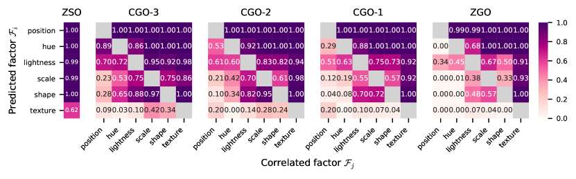
(a)

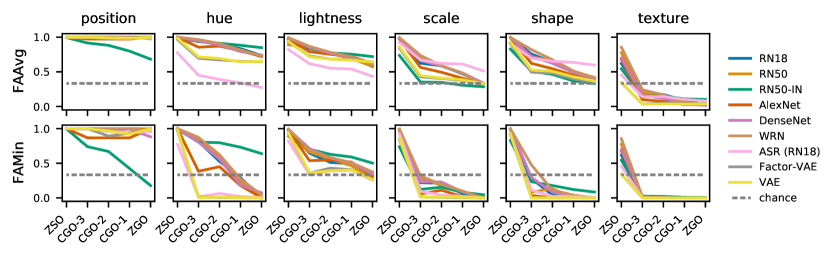
(b)

Figure 4: Best viewed in color. (a) For the RN18 baseline, we show mean accuracies $\text{P}_{i}$ for all factors $\mathcal{F}_{i}$ on the ZSO study and mean accuracies $\text{P}_{i,j}$ for all factor pairings $(\mathcal{F}_{i},\mathcal{F}_{j}),i\neq j$ on the CGO-c and ZGO studies. (b) Aggregating model behavior over the studies, we compare all baselines using our benchmark metrics FAAvg and FAMin. Note that in (b) error bars are omitted to improve visibility of individual baselines; standard errors are reported in Sec. A.3 and A.4.

3.4 Metrics

We benchmark a model on the studies described above, starting with evaluating the mean per-class accuracy $\text{acc}_{i,j}$ for the factor pair $(\mathcal{F}_{i},\mathcal{F}_{j})$, $i,j\in\{1,\ldots,6\}$, $i\neq j$, where $\mathcal{F}_{i}$ gets predicted. We define the prediction accuracy $\text{P}_{i,j}$ on the test dataset in a given study as the expectation over the five corresponding dataset samples: $\text{P}_{i,j}=\mathbb{E}\left[\text{acc}_{i,j}\right]$. In the case of ZSO, the prediction accuracy of $\mathcal{F}_{i}$ is defined as $\text{P}_{i}=\mathbb{E}\left[\text{acc}_{i}\right]$, with $\text{acc}_{i}$ being the accuracy of predicting $\mathcal{F}_{i}$ on a single dataset sample. We also define two different metrics to summarize a factor’s shortcut vulnerability with respect to the other factors:

i) The Factor-Aggregated Average accuracy (FAAvg)

$$\text{FAAvg}_{i}=\mathbb{E}\left[\underset{j\in\{1,\ldots,6\},j\neq i}{\text{mean}}\text{acc}_{i,j}\right]$$ (1)

measures the average accuracy of predicting factor $\mathcal{F}_{i}$ over all possible correlations with other factors $\mathcal{F}_{j},j\in\{1,\ldots,6\},j\neq i$. It can also be seen as a measure of the average shortcut vulnerability of the factor on a given study.

ii) The Factor-Aggregated Minimum accuracy (FAMin)

$$\text{FAMin}_{i} =\mathbb{E}\left[\underset{j\in\{1,\ldots,6\},j\neq i}{\text{min}}\text{acc}_{i,j}\right]\vspace{-0.5em}$$ (2)

measures the minimum accuracy among the correlations, and can therefore be used as a measure of the maximum shortcut vulnerability of the factor on a given study. In the case of ZSO, $\text{FAAvg}_{i}=\text{FAMin}_{i}=\text{P}_{i}$.

4 Baseline setup

This section provides an overview of the baseline network architectures we evaluate on our benchmark. We consider popular, vision-based DNN architectures (not pretrained) from PyTorch’s torchvision package [30]: AlexNet [21], ResNet18 (RN18), ResNet50 (RN50) [10], Wide ResNet50-2 (WideRN) [37], and DenseNet-161 [14]. We also include RN50 with pretrained weights on ImageNet [5] (RN50-IN), with frozen convolutional layers and a randomly initialized fully connected layer to adapt to our benchmark. We also use the prior work Automatic Shortcut Removal (ASR) [26] as a baseline for our studies. In addition, since generative models, in particular those with interpretable factorised latent representations, are promising approaches to overcome shortcut learning on classification tasks [7], we evaluate a standard VAE [19] and a Factor-VAE [17] on our benchmark. More details on the training and setup of baselines are provided in Sec. A.2.

5 Results

We evaluate the baselines described in Sec. 4 on our benchmark suite described in Sec. 3.3. We start with the extreme cases of zero SO (ZSO) and zero GO (ZGO), followed by the other studies that introduce compositional and frequency-based GO to the training dataset.

ZSO and ZGO

Results for the ResNet18 baseline on both these studies are presented in Fig. 4(a). A comparison of all baselines using the metrics described in Sec. 3.4 is provided in Fig. 4(b). The factor-wise results for each baseline are presented in Sec. A.3 and A.4.

The ZSO study evaluates how well a model can predict each factor in the absence of SO. This yields a single mean accuracy $\text{P}_{i}$ for each factor $\mathcal{F}_{i}$, visualized as a vector on the very left in Fig. 4(a). Here, RN18 achieves high accuracies ($\geq$99\text{\,}\mathrm{\char 37\relax}$$) for predicting all factors except texture, for which the mean accuracy is lower $62\pm 6.\text{\,}\mathrm{\char 37\relax}$. A similar behavior can be observed for most other baselines (leftmost point in each plot of Fig. 4(b)) with a few exceptions: VAE, Factor-VAE and ASR are worse at predicting texture, with $34\text{\,}\mathrm{\char 37\relax}$, $34\text{\,}\mathrm{\char 37\relax}$, and $45\text{\,}\mathrm{\char 37\relax}$ accuracy, respectively. This is likely due to a limited capability in representing high-frequency structures (Sec. A.3). In summary, considering the aforementioned exceptions, all baselines can predict all factors to a reasonable extent.

The ZGO study evaluates a model’s ability to predict a factor $\mathcal{F}_{i}$ when each of its three factor classes co-occurs exclusively with a certain factor class of another factor $\mathcal{F}_{j}$ during training. Each such pairing $(\mathcal{F}_{i},\mathcal{F}_{j})$ corresponds to a single cell in the rightmost matrix plot in Fig. 4(a), where $\mathcal{F}_{i}$ are the rows and $\mathcal{F}_{j}$ are the columns. The color coded value in each cell indicates mean accuracy $\text{P}_{i,j},~{}i\neq j$ on OOD test samples, for which this correlation is violated.

For RN18, we observe that for some factor combinations (e.g. $(\mathcal{F}_{i},\mathcal{F}_{j})$: (shape, texture)) the model does not exploit the provided SO, and instead preferentially learns the actual task, leading to similar mean accuracies on OOD test samples compared to the corresponding ZSO accuracies for this factor. On the other hand, for other factor combinations (e.g. (texture, shape)) the model does exploit the provided SO, yielding OOD accuracies close to zero thus below chance level. texture and position factors play a special role: While position is exploited as a shortcut when predicting any other factor, texture is never exploited as shortcut, but is easy to shortcut by any other factor. Interestingly, $\text{P}_{i,j}\approx 1-\text{P}_{j,i}$ seems to hold for all factor combinations, i.e., if $\mathcal{F}_{i}$ is exploited as a shortcut for predicting $\mathcal{F}_{j}$, then $\mathcal{F}_{j}$ is not exploited as shortcut for predicting $\mathcal{F}_{i}$.

We argue that during training either (a) the representation gets dominated by a single factor ignoring the other or (b) is a superposition of both factors, i.e., both factors share capacity of the representation. The extent a factor is represented depends on its overall ”difficulty”, i.e., texture appears relatively difficult to learn, and how strongly $\mathcal{F}_{i}$ and $\mathcal{F}_{j}$ compete over the same capacities. During testing, $P_{i,j}\approx 1-P_{j,i}$ holds now for (a) but not for (b). For lightness and position, ZGO findings indicate (b), and a superposition of both factors is learnt, utilising different capacities.

This yields a dataset-dependent ranking among factors, which we use to order the rows of plots in Fig. 4(a), starting with the most shortcut-robust factor position, and ending with the most shortcut-vulnerable factor texture. Since a model’s ability to represent a factor in the presence of SO is related to its inductive bias, the ZGO study could be used to diagnose the efficiency of inductive biases of vision models in future work.

ZSO and ZGO findings transfer to most baselines, with a few exceptions: On RN50-IN, position is less often exploited as shortcut; the model instead exploits hue as shortcut when predicting position (Sec. A.4, matrix plots).

CGO

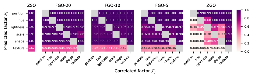
(a)

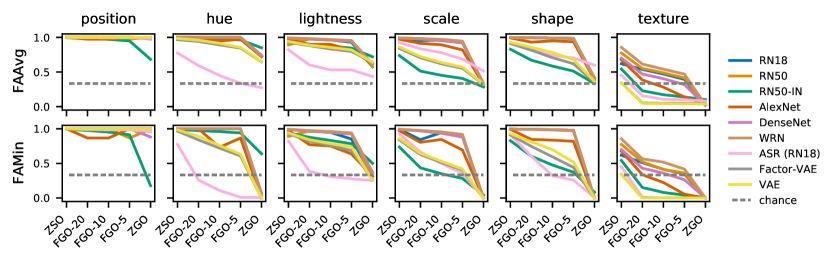
(b)

Figure 5: Best viewed in color. Similar to Fig. 4(a) and 4(b), we show mean accuracies for the RN18 (a) and a comparison of all baselines (b) on the ZSO, FGO and ZGO studies. Error estimates are provided in Sec. A.3 and A.5.

We now evaluate the capability of common vision models to exploit GO provided in the form of additional factor-class combinations. Here, the three benchmark datasets (CGO-1,2,3) successively add factor-class combinations to the ZGO study. Results for RN18 are shown in Fig. 4(a), and a comparison of all baselines using aggregated metrics is presented in Fig. 4(b). The factor-wise results for each baseline are shown in Sec. A.4.

For RN18, we find that most factor combinations exhibit a monotonic improvement with increasing number of GO, e.g. $(\texttt{scale},\texttt{hue}):0.01,0.19,0.42,0.53$ for ZGO, CGO-1,2,3, respectively. However, for some factor combinations the accuracy on OOD cases does not improve with an increasing number of GO, and for some factor combinations, e.g. $(\texttt{texture},\texttt{hue})$ or $(\texttt{shape},\texttt{position})$ shortcut learning occurs also for CGO-3.

This can also be seen for RN18 in the two aggregated benchmark metrics FAAvg and FAMin in Fig. 4(b). We find that FAAvg stays far below ZSO accuracy for most baselines up until three GO are added. For texture, FAAvg is below chance level for all baselines and studies, reflecting our earlier finding that all other factors are exploited as shortcuts when predicting texture. Moreover, FAMin stays below chance level for all baselines for texture, shape and scale factors, up until three GO are added.

In contrast to texture, for position, none of the baselines exploit shortcuts, with RN50-IN being the only exception (Fig. 4(b), leftmost column). This phenomenon is likely due to ImageNet containing limited explicit localization information [9], facilitating a partial invariance of the learned representations in RN50-IN. From the CGO study, we conclude that all baselines are unable to exploit compositional-based GO for most FoV used in this work.

CHGO

	pos.	hue	lightn.	scale	shape	text.
RN18	$0\pm 0.$	$2\pm 3.$	$27\pm 21.$	$-1\pm 14.$	$2\pm 5.$	$-1\pm 2.$
RN50	$0\pm 0.$	$3\pm 5.$	$26\pm 21.$	$-1\pm 16.$	$2\pm 5.$	$-2\pm 2.$
RN50-IN	$-1\pm 11.$	$5\pm 6.$	$15\pm 17.$	$-7\pm 11.$	$0\pm 8.$	$-1\pm 1.$
AlexNet	$-4\pm 8.$	$1\pm 4.$	$24\pm 19.$	$-1\pm 12.$	$3\pm 6.$	$-2\pm 2.$
DenseNet	$2\pm 3.$	$-3\pm 5.$	$24\pm 21.$	$-3\pm 13.$	$2\pm 5.$	$-1\pm 1.$
WRN	$1\pm 1.$	$-2\pm 4.$	$23\pm 22.$	$1\pm 14.$	$3\pm 6.$	$-2\pm 2.$
ASR	$1\pm 1.$	$12\pm 15.$	$32\pm 18.$	$1\pm 15.$	$1\pm 2.$	$0\pm 2.$
F-VAE	$0\pm 0.$	$2\pm 5.$	$19\pm 17.$	$-3\pm 11.$	$1\pm 8.$	$2\pm 1.$
VAE	$0\pm 0.$	$2\pm 5.$	$18\pm 15.$	$-3\pm 12.$	$0\pm 9.$	$2\pm 1.$

Table 2: Mean accuracy improvement and its standard deviation of the CHGO study over the ZGO study.

A special case of the CGO-2 study is the CHGO study, in which two classes of the predicted factor are provided with GO, while one class is presented with SO only (see Fig. 1 and 3). Comparing the accuracy on the OOD test samples for the latter with the average accuracy on the ZGO study (Tab. 2), we find no improvement for most factors on all baselines, and only minor improvements for lightness, albeit with large variance across the five dataset subsets. We conclude that all the baselines evaluated in this work do not transfer GO across classes.

FGO

An orthogonal approach to providing GO through additional class-combinations during training is to relax the strict correlation between factors by means of low-frequency violations of this correlation at training time. We generated three benchmark datasets (FGO-$f,~{}f\in\{5,10,20\}$), with $f$ indicating the frequency of the correlation violation at training time. Results for RN18 and a comparison of all baselines are presented in Fig. 5(a) and 5(b). The factor-wise results for each baseline are presented in Sec. A.5.

For the RN18, the classification for all factors improves significantly with only $5\text{\,}\mathrm{\char 37\relax}$ of the training samples for each class of the predicted factor violating the strict correlation from ZGO (e.g. $(\texttt{shape},\texttt{hue}):0.,0.98$ for ZGO and FGO-5, respectively). When $f\geq 10$, none of the factors except texture are vulnerable to shortcut learning. A similar behavior can be observed for most factors and baselines (Fig. 4(b)), where we find that FAAvg is above chance for all factors except texture for $f=5$. However, we find that ASR fails to exploit the presented GO for hue and lightness when compared to other baselines, a behavior which is likely attributed to the pixel-wise reconstruction loss that is used as a regularizer in the ASR objective. In summary, most baselines are able to exploit frequency-based GO to a certain extent on our benchmark.

6 Conclusion

We addressed the lack of a suitable benchmark to evaluate the shortcut behavior of vision models on a diverse set of basic visual FoV. To this end, we introduced DiagViB-6, a benchmark suite designed to evaluate two crucial model performance criteria: shortcut vulnerability and generalization capability. Our framework allows the user to create benchmark datasets by independently combining six visual FoV, thereby precisely controlling the SO and GO present in the dataset. Upon evaluation of the most commonly used vision architectures on DiagViB-6, we discovered that while they usually can exploit frequency-based GO, their ability to exploit compositional-based GO is limited. This finding also holds for some recent, promising approaches that have been proposed to overcome shortcut learning.

The design of DiagViB-6 is versatile, and leads to certain natural extensions. Three such promising future directions are: (a) including more complex correlation structures, potentially between more than two FoV; (b) transferring the benchmark design to other research areas like domain generalization and multitask learning; (c) extending to additional factors like background and natural corruptions. Lastly, we believe that our benchmark suite will inspire and help to build shortcut-robust solutions for vision models.

DiagViB-6: A Diagnostic Benchmark Suite for Vision Models in the Presence of Shortcut and Generalization Opportunities

Elias Eulig^1,2 Piyapat Saranrittichai^1,3 Chaithanya Kumar Mummadi^1,3
Kilian Rambach¹ William Beluch¹  Xiahan Shi¹  Volker Fischer^1
1Bosch Center for AI (BCAI) ²Heidelberg University ³University of Freiburg

Appendix A Supplementary material

A.1 Image generation

We provide a comprehensive overview of all factor classes and respective factor space regions in Tab. A1. The five textures from which the texture crops $f_{\text{text.}}$ are sampled are shown in Fig. A1.

$\mathcal{F}_{i}$	$\mathcal{S}_{i}$	$\mathcal{N}_{i}$	$\mathcal{C}_{i,j}$	$\mathcal{S}_{i,j}$
position	$[0,1]^{2}$	9	top-left	$[1/7,2/7]\times[1/7,2/7]$
			top-center	$[1/7,2/7]\times[3/7,4/7]$
			top-right	$[1/7,2/7]\times[5/7,6/7]$
			center-left	$[3/7,4/7]\times[1/7,2/7]$
			center-center	$[3/7,4/7]\times[3/7,4/7]$
			center-right	$[3/7,4/7]\times[5/7,6/7]$
			bottom-left	$[5/7,6/7]\times[1/7,2/7]$
			bottom-center	$[5/7,6/7]\times[3/7,4/7]$
			bottom-right	$[5/7,6/7]\times[5/7,6/7]$
hue	$[0,2\pi)$	6	red	$[$$,$$]$
			yellow	$[$$,$$]$
			green	$[$$,$$]$
			cyan	$[$$,$$]$
			blue	$[$$,$$]$
			magenta	$[$$,$$]$
lightness	$[0,1]^{2}$	4	dark	$[0,1/11]\times[4/11,5/11]$
			darker	$[2/11,3/11]\times[6/11,7/11]$
			brighter	$[4/11,5/11]\times[8/11,9/11]$
			bright	$[6/11,7/11]\times[10/11,1.]$
scale	$[1/1.45,1.45]$	5	small	$[1/1.45,1/1.35]$
			smaller	$[1/1.25,1/1.15]$
			normal	$[1/1.05,1.05]$
			larger	$[1.15,1.25]$
			large	$[1.35,1.45]$
shape	MNIST	10	‘0’	digits ‘0’
			‘1’	digits ‘1’
			$\vdots$	$\vdots$
texture	textures	5	tiles	tiles texture crops
			wood	wood texture crops
			carpet	carpet texture crops
			bricks	bricks texture crops
			lava	lava texture crops

Table A1: Overview of factors $\mathcal{F}_{i}$, respective factor spaces $\mathcal{S}_{i}$, number of classes $\mathcal{N}_{i}$, factor classes $\mathcal{C}_{i,j}$ and respective factor space regions $\mathcal{S}_{i,j}$ used in this work.

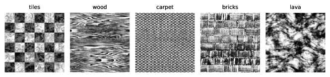
Figure A1: Overview of the textures used in this work. All textures are from CC0Textures.com, licensed under CC0 1.0 Universal.

A.2 Baselines

We train all baseline architectures using standard cross entropy loss and Adam optimizer [18] using early stopping. All test accuracies reported in this work correspond to the network with lowest validation loss. Batch size and learning rate were optimized on the ZSO study and weight initialization is fixed across all experiments. The output size of all the architectures are modified to predict the factor classes in our studies.

Following ASR, we use a variant of their U-Net architecture for the lens and ResNet18 as feature extractor. Instead of an auxiliary task, we train both the lens and feature extractor using the classification task directly. The lens is trained using least likely adversarial loss using the classification objective and also the reconstruction loss, both with equal weighting. Output of lens is used as inputs for training the feature extractor.

Both VAE methods use architectures similar to [25] with a latent size of $12$. We train both VAE with batch size $64$ and Adam optimizer [18] with learning rate $0.0001$. For the Factor-VAE, we use $\gamma=20$ and train the discriminator with learning rate $0.00001$ throughout our experiments. Some examples of latent traversals from VAE and Factor-VAE are shown in Fig. A2. We experimented with $\beta$-VAEs but observed, that the reconstructions of are poor when we use higher $\beta$ in our settings. One potential reason is the discretely distributed positions in the trained datasets. The position factor of DiagViB-6 has nine possible values with large gap among them violating the Gaussian distribution assumption in the KL-divergence term during training. To empirically demonstrate this claim, we train $\beta$-VAEs with different $\beta$ on two settings: (1) with position factor freely assigned to three different values (2) with position factor fixed to the center of the images. According to the results shown in Fig. A3, the reconstructions from the training with fixed position are significantly better, supporting the aforementioned argument.

A.3 ZSO and ZGO

The mean accuracies $\text{P}_{i}$ for all factors $\mathcal{F}_{i}$ on the ZSO together with the mean accuracies $\text{P}_{i,j}$ for all factor pairings $(\mathcal{F}_{i},\mathcal{F}_{j}),i\neq j$ on the ZGO study for all baselines are shown in Fig. A5 and A6. Additionally, the aggregated benchmark metrics $\text{FAAvg}_{i}$ and $\text{FAMin}_{i}$ for all factors $\mathcal{F}_{i},i\in\{0,1,...,6\}$ together with their respective standard errors for all baselines on the ZSO and ZGO studies are presented in Tab. A3 and A3.

From the exemplar VAE decoder reconstructions (Fig. A3) and ASR lens outputs (Fig. A4) we find that the high-frequency texture information is not preserved, leading to the observed low classification accuracies on the texture task.

A.4 Compositional-based generalization opportunities

The mean accuracies $\text{P}_{i}$ for all factors $\mathcal{F}_{i}$ on the ZSO together with the mean accuracies $\text{P}_{i,j}$ for all factor pairings $(\mathcal{F}_{i},\mathcal{F}_{j}),i\neq j$ on the CGO and ZGO studies for all baselines are shown in Fig. A5 and A6. Additionally, the aggregated benchmark metrics $\text{FAAvg}_{i}$ and $\text{FAMin}_{i}$ for all factors $\mathcal{F}_{i},i\in\{0,1,...,6\}$ together with their respective standard errors for all baselines on the CGO studies are presented in Tab. A6, A6 and A6.

A.5 Frequency-based generalization opportunities

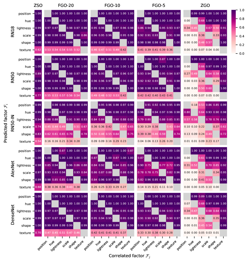
Figure A7: Mean accuracies $\text{P}_{i}$ for all factors $\mathcal{F}_{i}$ on the ZSO study and mean accuracies $\text{P}_{i,j}$ for all factor pairings $(\mathcal{F}_{i},\mathcal{F}_{j}),i\neq j$ for the RN18, RN50, RN50-IN, AlexNet and DenseNet on the FGO and ZGO studies.

The mean accuracies $\text{P}_{i}$ for all factors $\mathcal{F}_{i}$ on the ZSO together with the mean accuracies $\text{P}_{i,j}$ for all factor pairings $(\mathcal{F}_{i},\mathcal{F}_{j}),i\neq j$ on the FGO and ZGO studies for all baselines are shown in Fig. A7 and A8. Additionally, the aggregated benchmark metrics $\text{FAAvg}_{i}$ and $\text{FAMin}_{i}$ for all factors $\mathcal{F}_{i},i\in\{0,1,...,6\}$ together with their respective standard errors for all baselines on the FGO studies are presented in Tab. A9, A9 and A9.

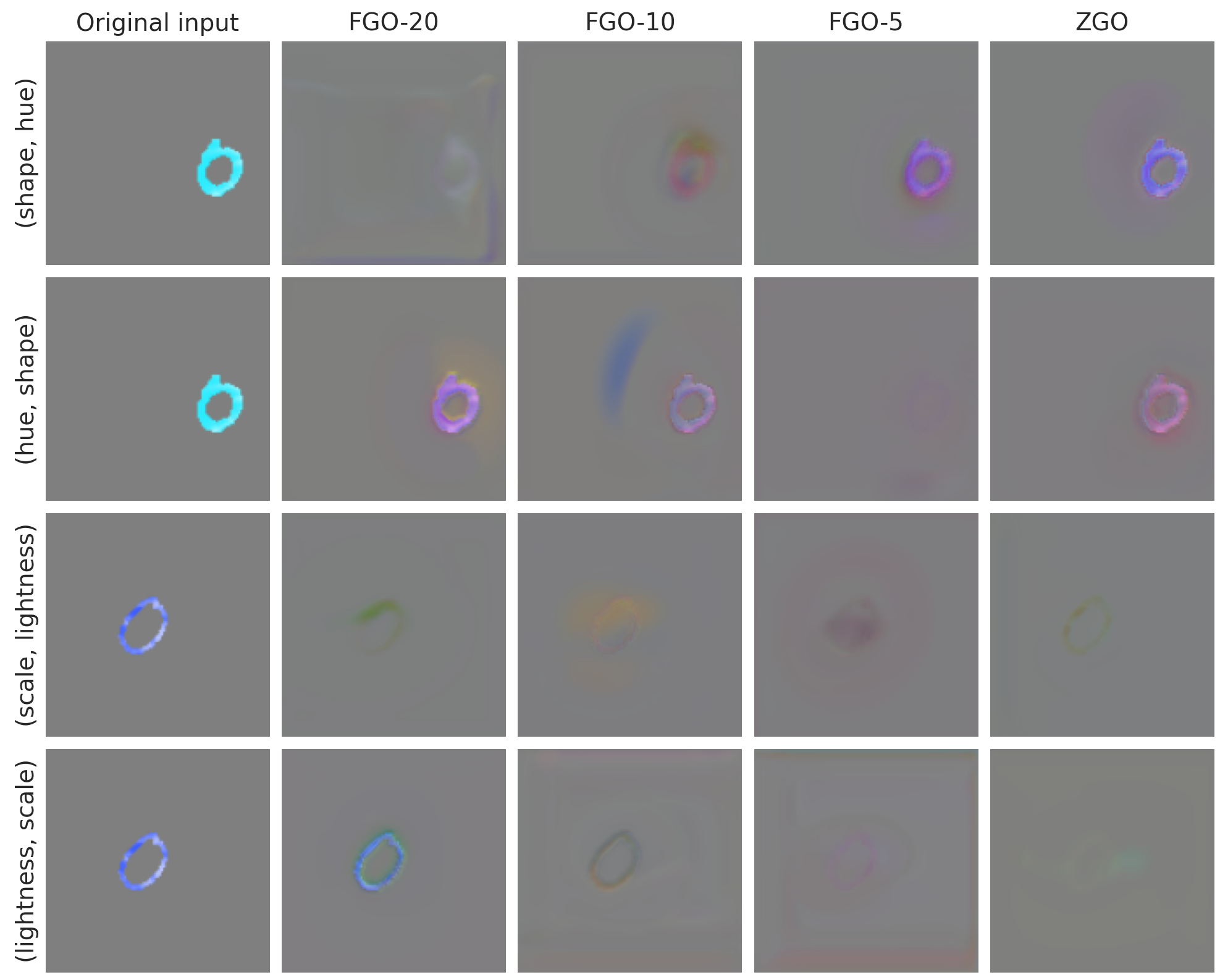
Figure A9: Examples of Automatic shortcut removal Lens output for different studies in our benchmark on datasets with following factor correlations: $(\texttt{shape},\texttt{hue})$ (first row), $(\texttt{hue},\texttt{shape})$ (second row), $(\texttt{scale},\texttt{lightness})$ (third row), $(\texttt{lightness},\texttt{scale})$ (fourth row).

As discussed in Sec. 5, we find that ASR fails to exploit the presented GO for hue and lightness. This is likely attributed to the pixel-wise reconstruction loss that is used as a regularizer in the ASR objective. We present qualitative results of this behaviour in Fig. A9.

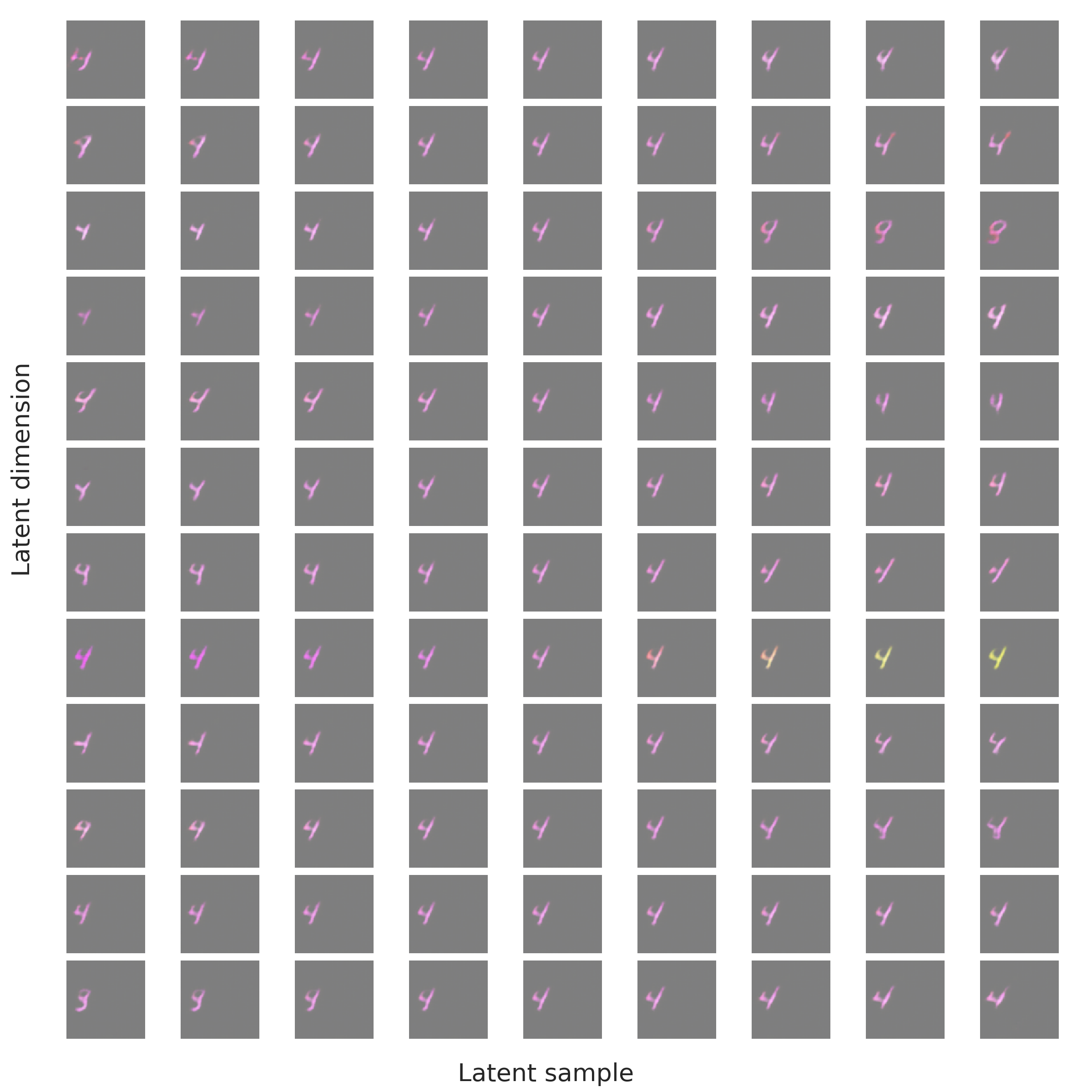
(a) Latent traversal plot from VAE

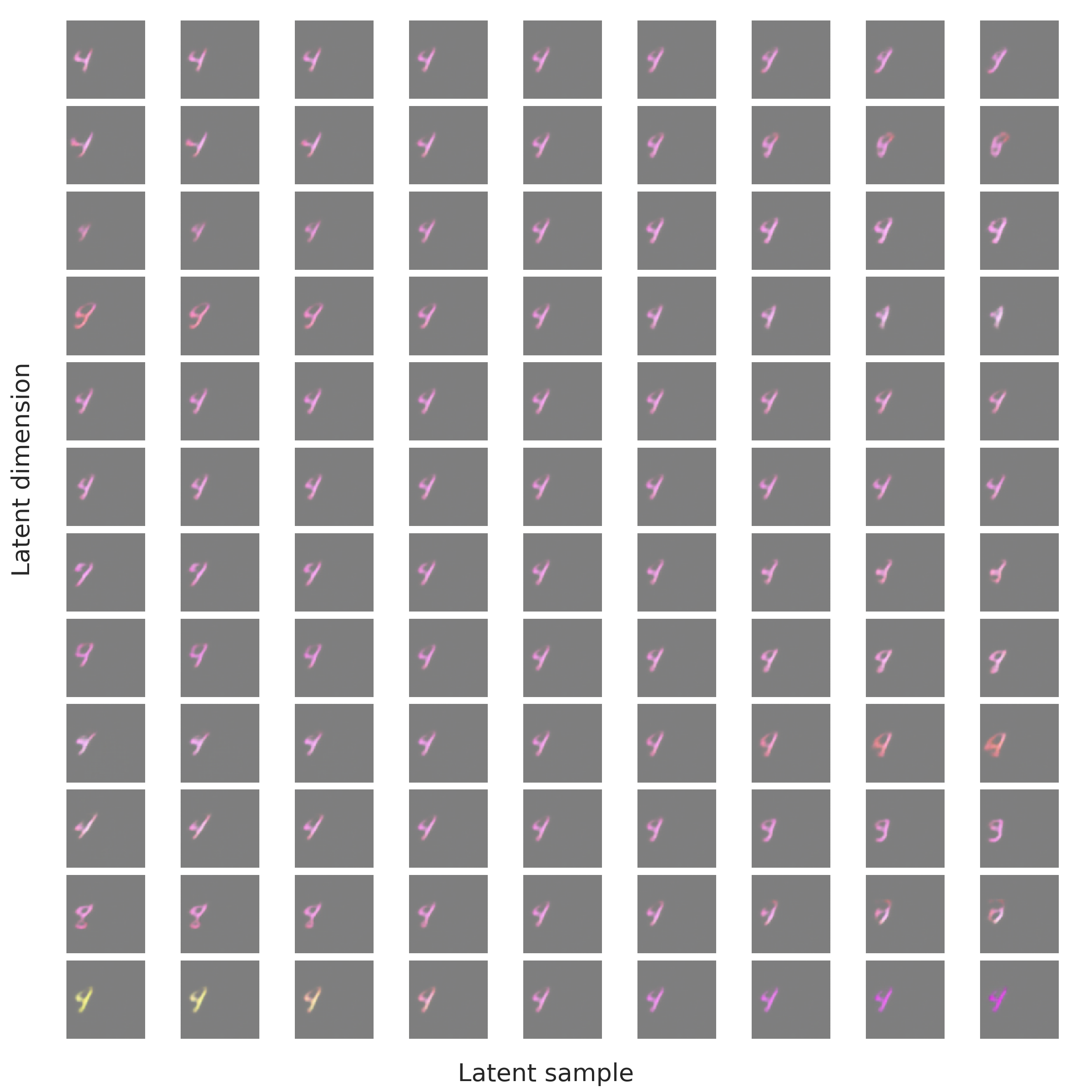
(b) Latent traversal plot from Factor-VAE

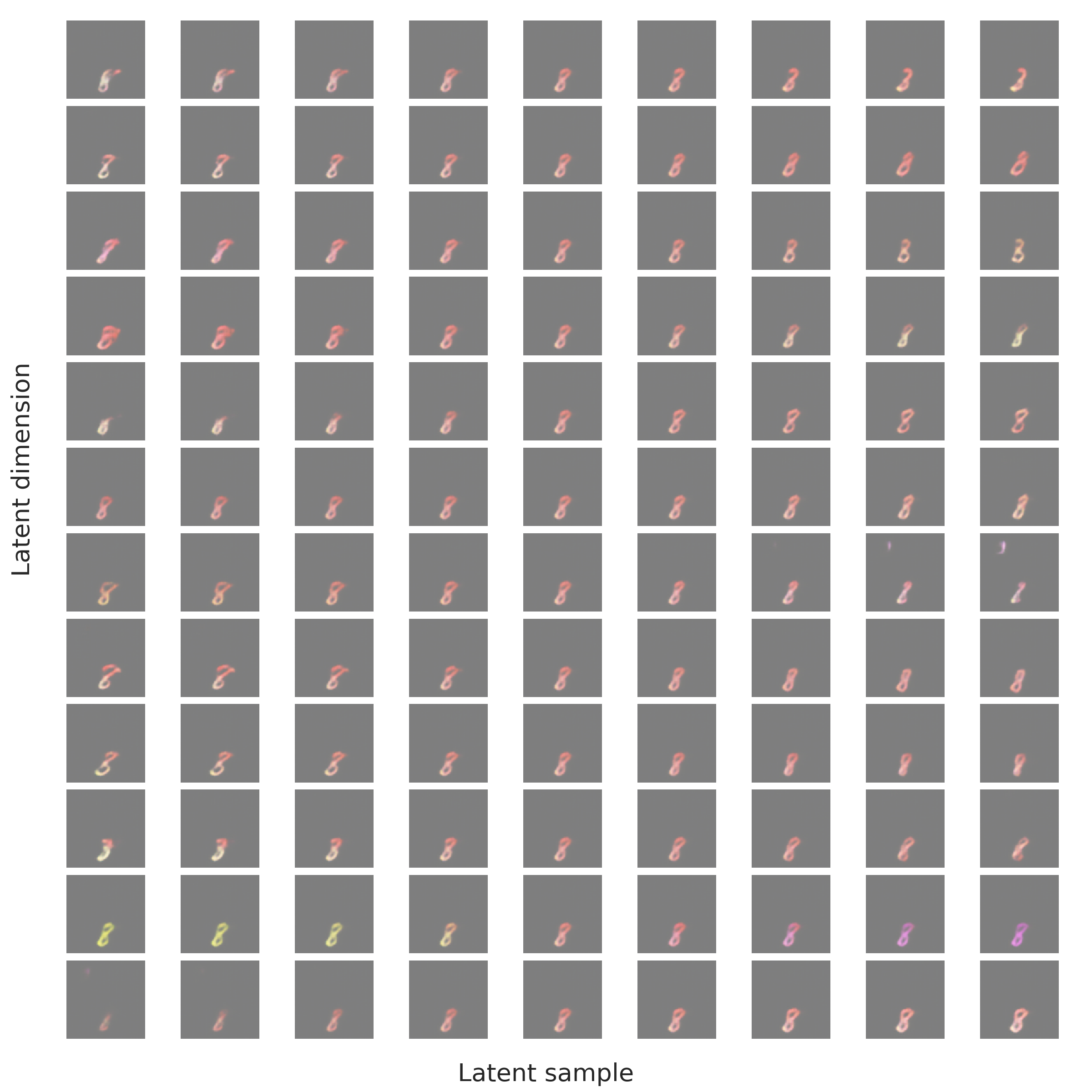
(c) Latent traversal plot from VAE

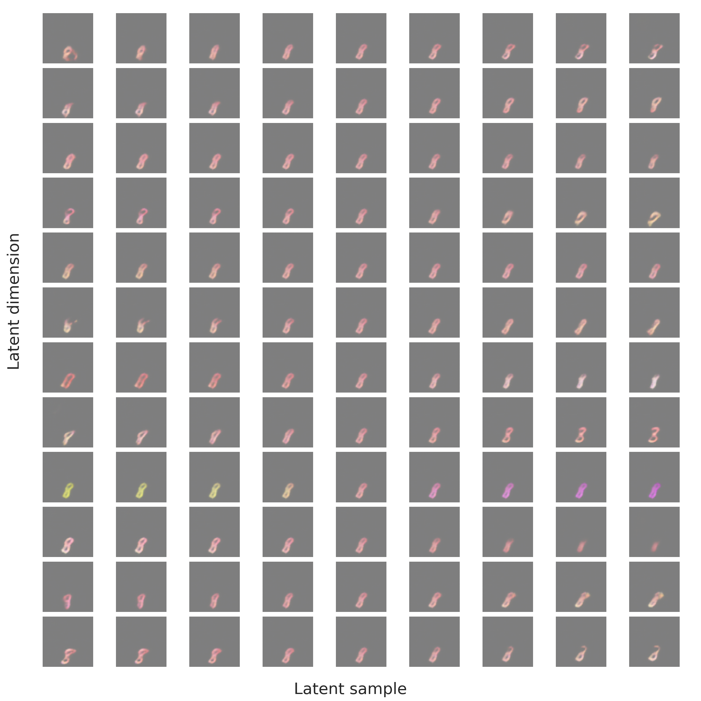
(d) Latent traversal plot from Factor-VAE

Figure A2: Comparison of latent traversals from VAE and Factor-VAE

(a) Input image (Sample 1)

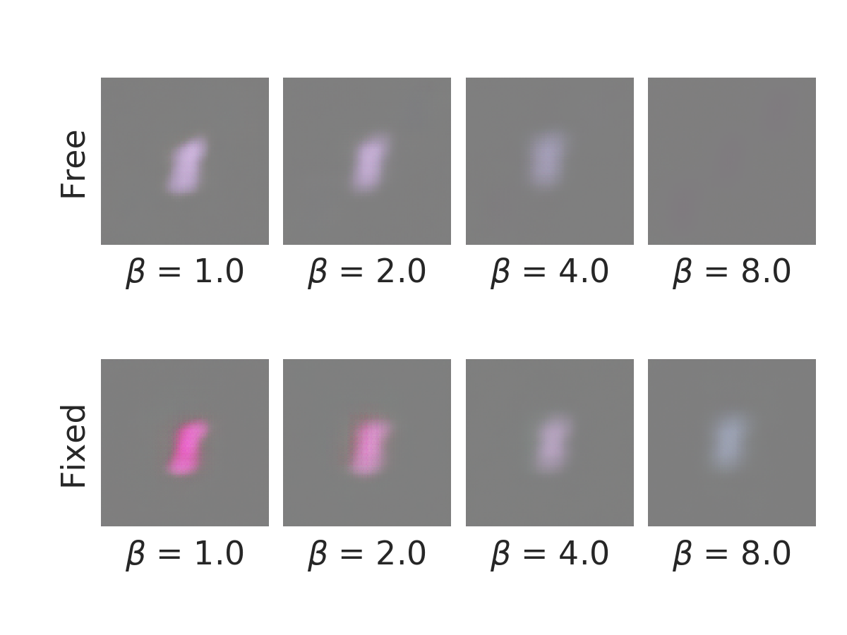
(b) Reconstructed images
(Sample 1)

(c) Input image (Sample 2)

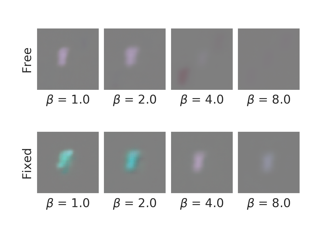
(d) Reconstructed images
(Sample 2)

(e) Input image (Sample 3)

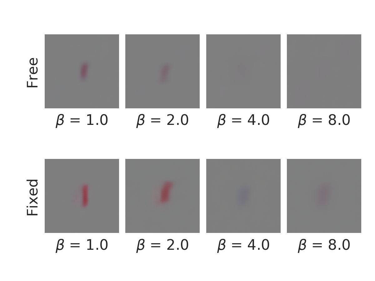
(f) Reconstructed images
(Sample 3)

(g) Input image (Sample 4)

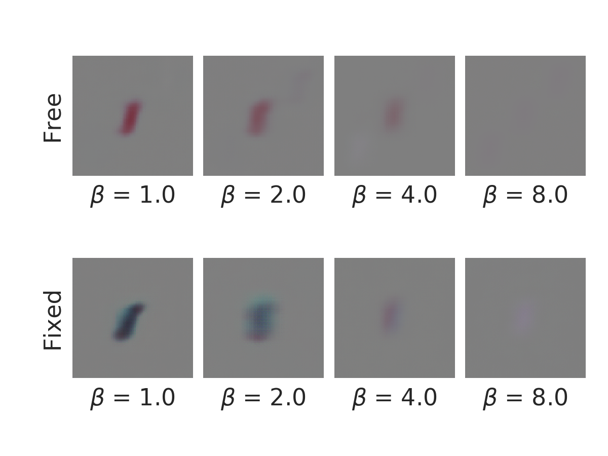
(h) Reconstructed images
(Sample 4)

Figure A3: Reconstruction images from the $\beta$-VAE networks trained with datasets of free and fixed positions from different $\beta$ values

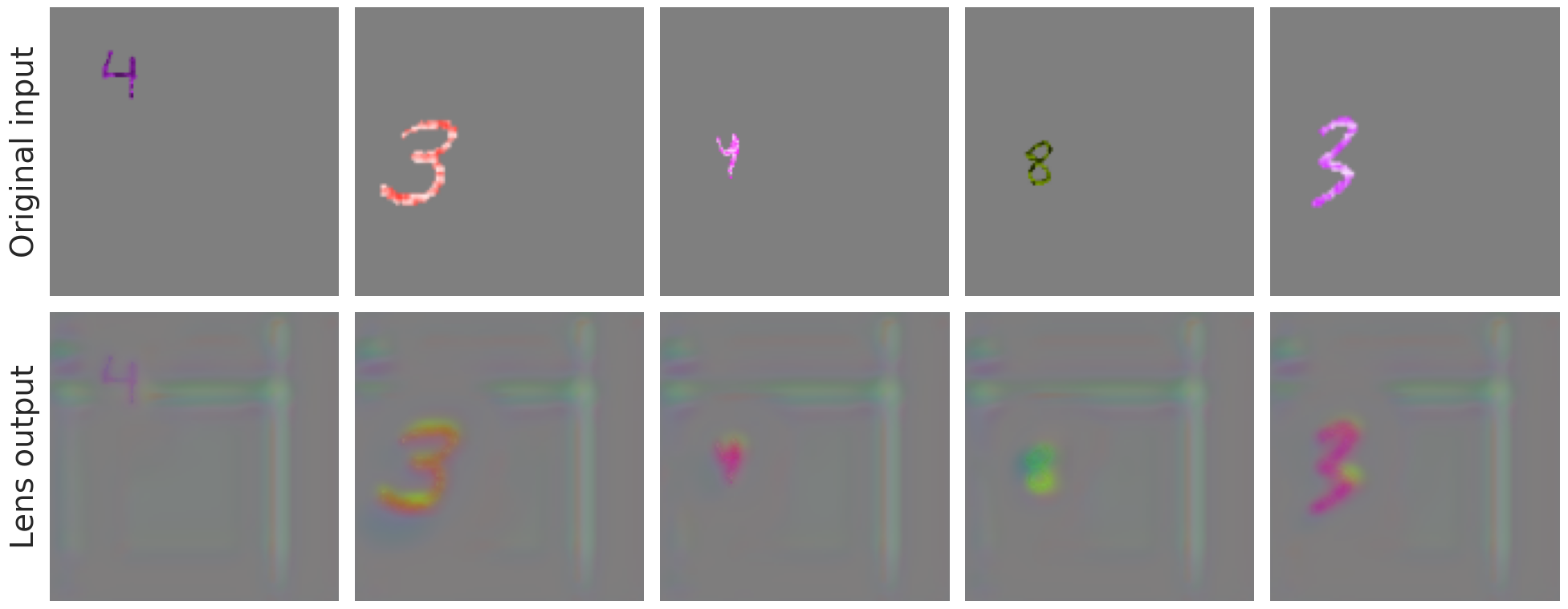
Figure A4: Examples of Automatic shortcut removal Lens output for ZSO study with factor texture.

	position	hue	lightness	scale	shape	texture
RN18	$100\pm 0.$	$100\pm 0.$	$99\pm 0.$	$99\pm 0.$	$100\pm 0.$	$62\pm 6.$
RN50	$100\pm 0.$	$100\pm 0.$	$89\pm 9.$	$99\pm 0.$	$100\pm 0.$	$77\pm 3.$
RN50-IN	$99\pm 0.$	$99\pm 0.$	$94\pm 1.$	$74\pm 2.$	$83\pm 3.$	$54\pm 1.$
AlexNet	$100\pm 0.$	$100\pm 0.$	$98\pm 1.$	$97\pm 0.$	$99\pm 0.$	$68\pm 3.$
DenseNet	$100\pm 0.$	$100\pm 0.$	$99\pm 0.$	$99\pm 0.$	$100\pm 0.$	$70\pm 3.$
WRN	$100\pm 0.$	$100\pm 0.$	$99\pm 0.$	$99\pm 0.$	$100\pm 0.$	$86\pm 2.$
ASR (RN18)	$100\pm 0.$	$77\pm 6.$	$82\pm 2.$	$92\pm 1.$	$91\pm 1.$	$45\pm 1.$
Factor-VAE	$100\pm 0.$	$97\pm 1.$	$93\pm 2.$	$84\pm 1.$	$91\pm 2.$	$34\pm 0.$
VAE	$100\pm 0.$	$98\pm 1.$	$94\pm 1.$	$86\pm 2.$	$93\pm 2.$	$34\pm 0.$

Table A2: FAAvg and respecive standard error for all baselines on the ZSO study.

	position		hue		lightness		scale		shape		texture
	FAAvg	FAMin	FAAvg	FAMin	FAAvg	FAMin	FAAvg	FAMin	FAAvg	FAMin	FAAvg	FAMin
RN18	$100\pm 0.$	$99\pm 1.$	$74\pm 2.$	$0\pm 0.$	$57\pm 4.$	$31\pm 5.$	$33\pm 2.$	$0\pm 0.$	$41\pm 2.$	$0\pm 0.$	$2\pm 1.$	$0\pm 0.$
RN50	$100\pm 0.$	$100\pm 0.$	$72\pm 2.$	$0\pm 0.$	$58\pm 4.$	$27\pm 1.$	$32\pm 2.$	$0\pm 0.$	$42\pm 2.$	$0\pm 0.$	$3\pm 1.$	$0\pm 0.$
RN50-IN	$68\pm 3.$	$18\pm 2.$	$85\pm 2.$	$64\pm 3.$	$72\pm 4.$	$50\pm 6.$	$28\pm 2.$	$4\pm 1.$	$33\pm 5.$	$8\pm 4.$	$10\pm 1.$	$1\pm 0.$
AlexNet	$100\pm 0.$	$100\pm 0.$	$72\pm 2.$	$0\pm 0.$	$62\pm 6.$	$31\pm 5.$	$32\pm 2.$	$0\pm 0.$	$39\pm 2.$	$0\pm 0.$	$3\pm 1.$	$0\pm 0.$
DenseNet	$98\pm 1.$	$88\pm 6.$	$74\pm 3.$	$7\pm 3.$	$61\pm 6.$	$34\pm 8.$	$34\pm 1.$	$0\pm 0.$	$40\pm 2.$	$0\pm 0.$	$2\pm 0.$	$0\pm 0.$
WRN	$99\pm 1.$	$96\pm 3.$	$73\pm 3.$	$4\pm 3.$	$61\pm 6.$	$37\pm 8.$	$32\pm 2.$	$0\pm 0.$	$41\pm 2.$	$0\pm 0.$	$2\pm 1.$	$0\pm 0.$
ASR (RN18)	$99\pm 0.$	$96\pm 1.$	$27\pm 3.$	$1\pm 0.$	$43\pm 2.$	$25\pm 0.$	$51\pm 2.$	$0\pm 0.$	$60\pm 1.$	$1\pm 0.$	$8\pm 0.$	$0\pm 0.$
Factor-VAE	$100\pm 0.$	$100\pm 0.$	$65\pm 4.$	$0\pm 0.$	$64\pm 4.$	$27\pm 0.$	$32\pm 1.$	$0\pm 0.$	$35\pm 2.$	$0\pm 0.$	$4\pm 0.$	$0\pm 0.$
VAE	$100\pm 0.$	$100\pm 0.$	$65\pm 4.$	$0\pm 0.$	$64\pm 4.$	$26\pm 0.$	$33\pm 2.$	$0\pm 0.$	$37\pm 3.$	$0\pm 0.$	$4\pm 0.$	$0\pm 0.$

Table A3: FAAvg and FAMin together with their respective standard errors for all baselines on the ZGO study.

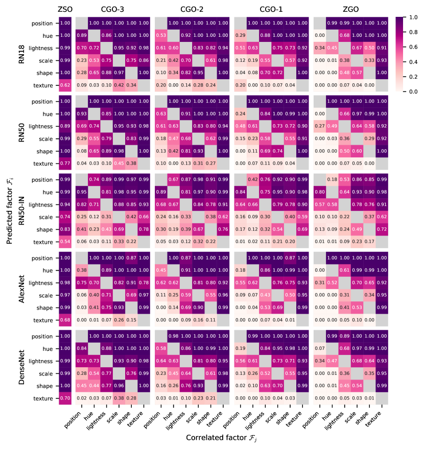
Figure A5: Mean accuracies $\text{P}_{i}$ for all factors $\mathcal{F}_{i}$ on the ZSO study and mean accuracies $\text{P}_{i,j}$ for all factor pairings $(\mathcal{F}_{i},\mathcal{F}_{j}),i\neq j$ for the RN18, RN50, RN50-IN, AlexNet and DenseNet on the CGO and ZGO studies.

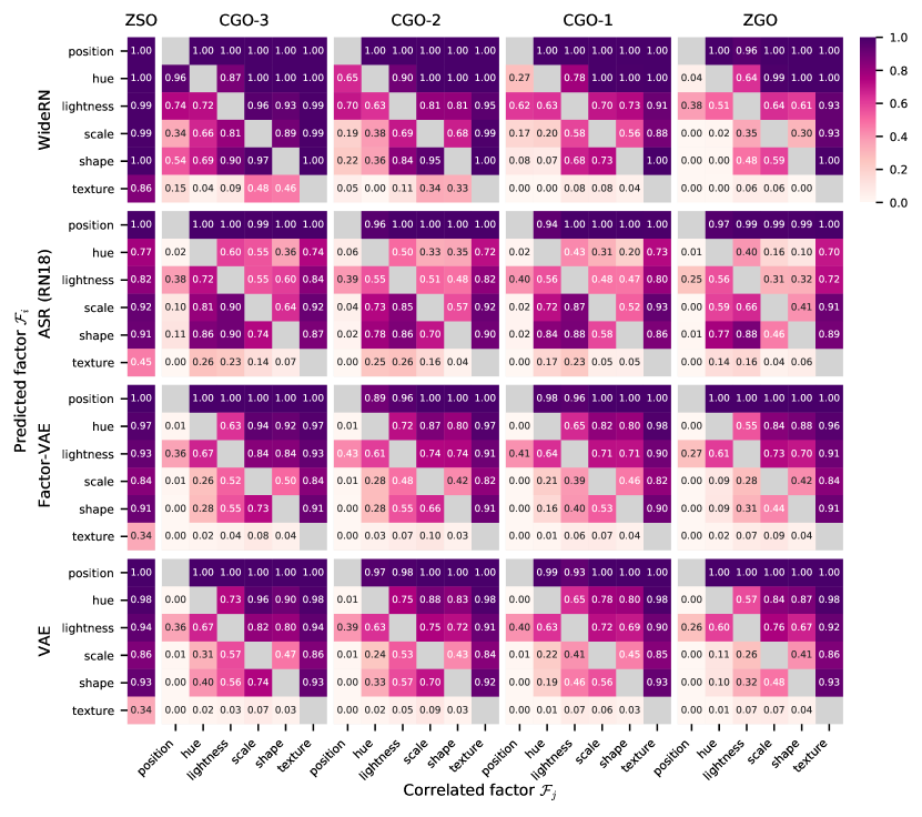
Figure A6: Mean accuracies $\text{P}_{i}$ for all factors $\mathcal{F}_{i}$ on the ZSO study and mean accuracies $\text{P}_{i,j}$ for all factor pairings $(\mathcal{F}_{i},\mathcal{F}_{j}),i\neq j$ for the WideRN, ASR (RN18), Factor-VAE and VAE on the CGO and ZGO studies.

	position		hue		lightness		scale		shape		texture
	FAAvg	FAMin	FAAvg	FAMin	FAAvg	FAMin	FAAvg	FAMin	FAAvg	FAMin	FAAvg	FAMin
RN18	$100\pm 0.$	$100\pm 0.$	$83\pm 1.$	$29\pm 5.$	$71\pm 8.$	$49\pm 9.$	$47\pm 3.$	$6\pm 2.$	$51\pm 3.$	$2\pm 1.$	$8\pm 2.$	$0\pm 0.$
RN50	$100\pm 0.$	$100\pm 0.$	$82\pm 1.$	$24\pm 6.$	$69\pm 8.$	$46\pm 8.$	$48\pm 4.$	$9\pm 3.$	$51\pm 3.$	$0\pm 0.$	$6\pm 2.$	$0\pm 0.$
RN50-IN	$80\pm 2.$	$42\pm 4.$	$88\pm 2.$	$73\pm 3.$	$75\pm 5.$	$59\pm 8.$	$31\pm 3.$	$8\pm 2.$	$37\pm 6.$	$12\pm 5.$	$11\pm 1.$	$1\pm 0.$
AlexNet	$97\pm 2.$	$87\pm 12.$	$81\pm 2.$	$18\pm 7.$	$72\pm 8.$	$52\pm 10.$	$41\pm 3.$	$2\pm 1.$	$45\pm 3.$	$0\pm 0.$	$3\pm 0.$	$0\pm 0.$
DenseNet	$100\pm 0.$	$99\pm 1.$	$79\pm 1.$	$19\pm 1.$	$71\pm 8.$	$50\pm 10.$	$48\pm 4.$	$9\pm 3.$	$49\pm 2.$	$2\pm 1.$	$3\pm 0.$	$0\pm 0.$
WRN	$100\pm 0.$	$100\pm 0.$	$81\pm 2.$	$27\pm 4.$	$72\pm 9.$	$51\pm 10.$	$48\pm 3.$	$10\pm 3.$	$51\pm 3.$	$4\pm 2.$	$4\pm 1.$	$0\pm 0.$
ASR (RN18)	$99\pm 1.$	$94\pm 3.$	$34\pm 3.$	$2\pm 1.$	$54\pm 4.$	$40\pm 5.$	$61\pm 2.$	$2\pm 1.$	$64\pm 3.$	$2\pm 1.$	$10\pm 1.$	$0\pm 0.$
Factor-VAE	$99\pm 0.$	$93\pm 2.$	$65\pm 3.$	$0\pm 0.$	$67\pm 6.$	$41\pm 5.$	$38\pm 3.$	$0\pm 0.$	$40\pm 3.$	$0\pm 0.$	$4\pm 0.$	$0\pm 0.$
VAE	$98\pm 1.$	$92\pm 3.$	$64\pm 3.$	$0\pm 0.$	$67\pm 6.$	$40\pm 6.$	$39\pm 3.$	$1\pm 0.$	$43\pm 4.$	$0\pm 0.$	$3\pm 0.$	$0\pm 0.$

Table A4: Aggregated benchmark metrics $\text{FAAvg}_{i}$ and $\text{FAMin}_{i}$ for all factors $\mathcal{F}_{i},i\in\{0,1,...,6\}$ together with their respective standard errors for all baselines on the CGO-1 study.

	position		hue		lightness		scale		shape		texture
	FAAvg	FAMin	FAAvg	FAMin	FAAvg	FAMin	FAAvg	FAMin	FAAvg	FAMin	FAAvg	FAMin
RN18	$100\pm 0.$	$100\pm 0.$	$89\pm 4.$	$53\pm 16.$	$76\pm 11.$	$51\pm 14.$	$59\pm 5.$	$21\pm 6.$	$64\pm 2.$	$4\pm 2.$	$17\pm 4.$	$0\pm 0.$
RN50	$100\pm 0.$	$100\pm 0.$	$91\pm 4.$	$59\pm 17.$	$76\pm 10.$	$56\pm 14.$	$59\pm 4.$	$18\pm 7.$	$66\pm 3.$	$13\pm 5.$	$16\pm 4.$	$0\pm 0.$
RN50-IN	$88\pm 2.$	$67\pm 6.$	$91\pm 3.$	$80\pm 4.$	$77\pm 8.$	$63\pm 12.$	$35\pm 5.$	$15\pm 4.$	$46\pm 6.$	$18\pm 5.$	$15\pm 2.$	$2\pm 1.$
AlexNet	$97\pm 2.$	$87\pm 12.$	$87\pm 2.$	$45\pm 7.$	$75\pm 9.$	$55\pm 14.$	$49\pm 4.$	$11\pm 5.$	$55\pm 2.$	$0\pm 0.$	$7\pm 2.$	$0\pm 0.$
DenseNet	$100\pm 0.$	$98\pm 2.$	$89\pm 4.$	$56\pm 14.$	$77\pm 10.$	$58\pm 15.$	$58\pm 5.$	$23\pm 4.$	$62\pm 2.$	$8\pm 3.$	$12\pm 3.$	$0\pm 0.$
WRN	$100\pm 0.$	$100\pm 0.$	$91\pm 4.$	$62\pm 17.$	$78\pm 11.$	$58\pm 14.$	$59\pm 4.$	$19\pm 3.$	$67\pm 3.$	$11\pm 6.$	$17\pm 4.$	$0\pm 0.$
ASR (RN18)	$99\pm 1.$	$96\pm 3.$	$39\pm 6.$	$6\pm 6.$	$55\pm 7.$	$39\pm 9.$	$62\pm 2.$	$4\pm 2.$	$65\pm 3.$	$2\pm 1.$	$14\pm 2.$	$0\pm 0.$
Factor-VAE	$97\pm 2.$	$89\pm 6.$	$67\pm 4.$	$1\pm 0.$	$68\pm 8.$	$43\pm 10.$	$40\pm 4.$	$1\pm 0.$	$48\pm 3.$	$0\pm 0.$	$5\pm 1.$	$0\pm 0.$
VAE	$99\pm 1.$	$97\pm 3.$	$69\pm 4.$	$1\pm 0.$	$68\pm 7.$	$39\pm 8.$	$41\pm 4.$	$1\pm 0.$	$51\pm 4.$	$0\pm 0.$	$4\pm 0.$	$0\pm 0.$

Table A5: Aggregated benchmark metrics $\text{FAAvg}_{i}$ and $\text{FAMin}_{i}$ for all factors $\mathcal{F}_{i},i\in\{0,1,...,6\}$ together with their respective standard errors for all baselines on the CGO-2 study.

	position		hue		lightness		scale		shape		texture
	FAAvg	FAMin	FAAvg	FAMin	FAAvg	FAMin	FAAvg	FAMin	FAAvg	FAMin	FAAvg	FAMin
RN18	$100\pm 0.$	$100\pm 0.$	$95\pm 3.$	$81\pm 9.$	$86\pm 6.$	$65\pm 13.$	$62\pm 7.$	$22\pm 3.$	$76\pm 3.$	$28\pm 7.$	$19\pm 4.$	$1\pm 0.$
RN50	$100\pm 0.$	$100\pm 0.$	$96\pm 2.$	$85\pm 8.$	$86\pm 7.$	$66\pm 17.$	$69\pm 7.$	$29\pm 9.$	$72\pm 2.$	$8\pm 3.$	$20\pm 4.$	$1\pm 0.$
RN50-IN	$92\pm 2.$	$74\pm 7.$	$94\pm 1.$	$81\pm 5.$	$84\pm 5.$	$70\pm 10.$	$35\pm 5.$	$12\pm 3.$	$51\pm 8.$	$23\pm 10.$	$15\pm 2.$	$3\pm 1.$
AlexNet	$97\pm 2.$	$87\pm 12.$	$86\pm 2.$	$38\pm 7.$	$79\pm 7.$	$54\pm 11.$	$56\pm 7.$	$6\pm 2.$	$62\pm 4.$	$3\pm 2.$	$10\pm 2.$	$0\pm 0.$
DenseNet	$100\pm 0.$	$100\pm 0.$	$94\pm 2.$	$80\pm 6.$	$86\pm 7.$	$71\pm 13.$	$66\pm 7.$	$23\pm 4.$	$72\pm 4.$	$29\pm 11.$	$16\pm 3.$	$1\pm 0.$
WRN	$100\pm 0.$	$100\pm 0.$	$97\pm 2.$	$87\pm 6.$	$87\pm 6.$	$69\pm 13.$	$74\pm 6.$	$32\pm 7.$	$82\pm 3.$	$48\pm 9.$	$24\pm 6.$	$2\pm 0.$
ASR (RN18)	$100\pm 0.$	$99\pm 0.$	$45\pm 1.$	$2\pm 1.$	$62\pm 8.$	$34\pm 8.$	$67\pm 3.$	$10\pm 5.$	$69\pm 3.$	$11\pm 7.$	$14\pm 1.$	$0\pm 0.$
Factor-VAE	$100\pm 0.$	$100\pm 0.$	$70\pm 3.$	$1\pm 1.$	$73\pm 6.$	$36\pm 7.$	$43\pm 4.$	$1\pm 1.$	$49\pm 3.$	$0\pm 0.$	$4\pm 1.$	$0\pm 0.$
VAE	$100\pm 0.$	$100\pm 0.$	$72\pm 3.$	$0\pm 0.$	$72\pm 7.$	$36\pm 8.$	$44\pm 5.$	$1\pm 0.$	$53\pm 4.$	$0\pm 0.$	$3\pm 1.$	$0\pm 0.$

Table A6: Aggregated benchmark metrics $\text{FAAvg}_{i}$ and $\text{FAMin}_{i}$ for all factors $\mathcal{F}_{i},i\in\{0,1,...,6\}$ together with their respective standard errors for all baselines on the CGO-3 study.

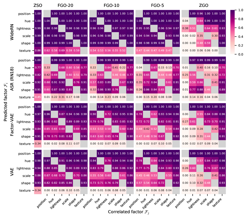
Figure A8: Mean accuracies $\text{P}_{i}$ for all factors $\mathcal{F}_{i}$ on the ZSO study and mean accuracies $\text{P}_{i,j}$ for all factor pairings $(\mathcal{F}_{i},\mathcal{F}_{j}),i\neq j$ for the WideRN, ASR (RN18), Factor-VAE and VAE on the FGO and ZGO studies.

	position		hue		lightness		scale		shape		texture
	FAAvg	FAMin	FAAvg	FAMin	FAAvg	FAMin	FAAvg	FAMin	FAAvg	FAMin	FAAvg	FAMin
RN18	$100\pm 0.$	$100\pm 0.$	$100\pm 0.$	$100\pm 0.$	$93\pm 2.$	$85\pm 8.$	$93\pm 1.$	$89\pm 1.$	$99\pm 0.$	$98\pm 0.$	$39\pm 2.$	$35\pm 3.$
RN50	$97\pm 2.$	$87\pm 12.$	$100\pm 0.$	$100\pm 0.$	$95\pm 1.$	$93\pm 2.$	$93\pm 1.$	$90\pm 1.$	$99\pm 0.$	$98\pm 0.$	$41\pm 2.$	$36\pm 1.$
RN50-IN	$95\pm 1.$	$91\pm 2.$	$96\pm 1.$	$94\pm 1.$	$85\pm 3.$	$78\pm 4.$	$41\pm 4.$	$28\pm 4.$	$51\pm 8.$	$37\pm 9.$	$14\pm 1.$	$4\pm 1.$
AlexNet	$100\pm 0.$	$100\pm 0.$	$97\pm 2.$	$87\pm 12.$	$82\pm 4.$	$64\pm 8.$	$82\pm 3.$	$69\pm 8.$	$94\pm 3.$	$82\pm 11.$	$14\pm 2.$	$6\pm 3.$
DenseNet	$100\pm 0.$	$100\pm 0.$	$100\pm 0.$	$100\pm 0.$	$94\pm 1.$	$92\pm 2.$	$92\pm 1.$	$88\pm 1.$	$98\pm 0.$	$97\pm 1.$	$32\pm 2.$	$26\pm 2.$
WRN	$100\pm 0.$	$100\pm 0.$	$100\pm 0.$	$100\pm 0.$	$95\pm 1.$	$94\pm 1.$	$95\pm 1.$	$92\pm 1.$	$98\pm 0.$	$98\pm 0.$	$47\pm 3.$	$42\pm 2.$
ASR (RN18)	$99\pm 0.$	$98\pm 0.$	$34\pm 3.$	$1\pm 1.$	$53\pm 4.$	$28\pm 1.$	$69\pm 2.$	$35\pm 6.$	$70\pm 2.$	$26\pm 7.$	$10\pm 1.$	$0\pm 0.$
Factor-VAE	$100\pm 0.$	$100\pm 0.$	$84\pm 4.$	$61\pm 9.$	$80\pm 5.$	$69\pm 7.$	$55\pm 4.$	$40\pm 4.$	$62\pm 5.$	$44\pm 7.$	$5\pm 0.$	$0\pm 0.$
VAE	$100\pm 0.$	$100\pm 0.$	$86\pm 3.$	$63\pm 8.$	$82\pm 4.$	$74\pm 5.$	$57\pm 4.$	$42\pm 4.$	$68\pm 5.$	$52\pm 6.$	$4\pm 0.$	$0\pm 0.$

Table A7: Aggregated benchmark metrics $\text{FAAvg}_{i}$ and $\text{FAMin}_{i}$ for all factors $\mathcal{F}_{i},i\in\{0,1,...,6\}$ together with their respective standard errors for all baselines on the FGO-5 study.

	position		hue		lightness		scale		shape		texture
	FAAvg	FAMin	FAAvg	FAMin	FAAvg	FAMin	FAAvg	FAMin	FAAvg	FAMin	FAAvg	FAMin
RN18	$100\pm 0.$	$100\pm 0.$	$100\pm 0.$	$100\pm 0.$	$96\pm 1.$	$95\pm 1.$	$96\pm 1.$	$95\pm 1.$	$99\pm 0.$	$99\pm 0.$	$47\pm 3.$	$41\pm 4.$
RN50	$100\pm 0.$	$100\pm 0.$	$100\pm 0.$	$100\pm 0.$	$96\pm 1.$	$95\pm 1.$	$97\pm 0.$	$95\pm 1.$	$99\pm 0.$	$99\pm 0.$	$49\pm 3.$	$41\pm 2.$
RN50-IN	$97\pm 1.$	$95\pm 1.$	$97\pm 1.$	$96\pm 1.$	$87\pm 2.$	$83\pm 3.$	$45\pm 3.$	$35\pm 4.$	$59\pm 7.$	$48\pm 9.$	$17\pm 2.$	$8\pm 1.$
AlexNet	$97\pm 2.$	$87\pm 12.$	$95\pm 3.$	$73\pm 15.$	$90\pm 3.$	$75\pm 9.$	$89\pm 1.$	$85\pm 2.$	$95\pm 3.$	$84\pm 11.$	$28\pm 2.$	$22\pm 2.$
DenseNet	$100\pm 0.$	$100\pm 0.$	$100\pm 0.$	$100\pm 0.$	$96\pm 1.$	$95\pm 1.$	$95\pm 1.$	$94\pm 1.$	$99\pm 0.$	$98\pm 1.$	$40\pm 1.$	$36\pm 1.$
WRN	$100\pm 0.$	$100\pm 0.$	$100\pm 0.$	$100\pm 0.$	$97\pm 1.$	$96\pm 1.$	$97\pm 0.$	$95\pm 0.$	$99\pm 0.$	$99\pm 0.$	$54\pm 5.$	$52\pm 5.$
ASR (RN18)	$99\pm 0.$	$98\pm 0.$	$45\pm 4.$	$11\pm 4.$	$53\pm 3.$	$31\pm 2.$	$78\pm 1.$	$50\pm 3.$	$74\pm 4.$	$32\pm 7.$	$10\pm 0.$	$0\pm 0.$
Factor-VAE	$100\pm 0.$	$100\pm 0.$	$89\pm 3.$	$72\pm 9.$	$83\pm 4.$	$76\pm 6.$	$62\pm 4.$	$51\pm 5.$	$71\pm 5.$	$60\pm 5.$	$5\pm 0.$	$0\pm 0.$
VAE	$100\pm 0.$	$100\pm 0.$	$91\pm 2.$	$76\pm 7.$	$86\pm 3.$	$79\pm 5.$	$64\pm 4.$	$53\pm 4.$	$78\pm 5.$	$70\pm 6.$	$4\pm 0.$	$0\pm 0.$

Table A8: Aggregated benchmark metrics $\text{FAAvg}_{i}$ and $\text{FAMin}_{i}$ for all factors $\mathcal{F}_{i},i\in\{0,1,...,6\}$ together with their respective standard errors for all baselines on the FGO-10 study.

	position		hue		lightness		scale		shape		texture
	FAAvg	FAMin	FAAvg	FAMin	FAAvg	FAMin	FAAvg	FAMin	FAAvg	FAMin	FAAvg	FAMin
RN18	$100\pm 0.$	$100\pm 0.$	$100\pm 0.$	$100\pm 0.$	$98\pm 1.$	$97\pm 1.$	$95\pm 2.$	$84\pm 11.$	$99\pm 0.$	$99\pm 0.$	$54\pm 5.$	$51\pm 5.$
RN50	$100\pm 0.$	$100\pm 0.$	$100\pm 0.$	$100\pm 0.$	$98\pm 1.$	$97\pm 1.$	$98\pm 0.$	$98\pm 0.$	$100\pm 0.$	$99\pm 0.$	$55\pm 5.$	$52\pm 5.$
RN50-IN	$98\pm 0.$	$98\pm 1.$	$98\pm 0.$	$97\pm 1.$	$90\pm 2.$	$88\pm 2.$	$51\pm 3.$	$44\pm 3.$	$67\pm 6.$	$60\pm 7.$	$23\pm 2.$	$15\pm 2.$
AlexNet	$97\pm 2.$	$87\pm 12.$	$100\pm 0.$	$100\pm 0.$	$90\pm 4.$	$77\pm 10.$	$91\pm 3.$	$80\pm 11.$	$93\pm 5.$	$85\pm 11.$	$38\pm 2.$	$34\pm 2.$
DenseNet	$100\pm 0.$	$100\pm 0.$	$100\pm 0.$	$100\pm 0.$	$97\pm 1.$	$96\pm 1.$	$97\pm 0.$	$97\pm 0.$	$99\pm 0.$	$99\pm 0.$	$47\pm 3.$	$43\pm 3.$
WRN	$100\pm 0.$	$100\pm 0.$	$100\pm 0.$	$100\pm 0.$	$98\pm 0.$	$97\pm 1.$	$98\pm 0.$	$97\pm 0.$	$99\pm 0.$	$99\pm 0.$	$61\pm 5.$	$57\pm 6.$
ASR (RN18)	$100\pm 0.$	$99\pm 0.$	$59\pm 4.$	$26\pm 8.$	$60\pm 3.$	$38\pm 2.$	$84\pm 2.$	$67\pm 5.$	$82\pm 3.$	$60\pm 7.$	$16\pm 1.$	$1\pm 1.$
Factor-VAE	$100\pm 0.$	$100\pm 0.$	$94\pm 2.$	$84\pm 5.$	$88\pm 3.$	$82\pm 5.$	$71\pm 3.$	$63\pm 3.$	$81\pm 4.$	$75\pm 5.$	$5\pm 0.$	$0\pm 0.$
VAE	$100\pm 0.$	$100\pm 0.$	$96\pm 1.$	$89\pm 4.$	$89\pm 3.$	$84\pm 4.$	$72\pm 3.$	$65\pm 3.$	$85\pm 3.$	$81\pm 4.$	$5\pm 0.$	$0\pm 0.$

Table A9: Aggregated benchmark metrics $\text{FAAvg}_{i}$ and $\text{FAMin}_{i}$ for all factors $\mathcal{F}_{i},i\in\{0,1,...,6\}$ together with their respective standard errors for all baselines on the FGO-20 study.

References

- [1] Amit Alfassy, Leonid Karlinsky, Amit Aides, Joseph Shtok, Sivan Harary, Rogerio Feris, Raja Giryes, and Alex M. Bronstein. Laso: Label-set operations networks for multi-label few-shot learning. In IEEE/CVF Conference on Computer Vision and Pattern Recognition (CVPR), June 2019.
- [2] Yuval Atzmon, Felix Kreuk, Uri Shalit, and Gal Chechik. A causal view of compositional zero-shot recognition. Advances in Neural Information Processing Systems, 33, 2020.
- [3] Nicholas Baker, Hongjing Lu, Gennady Erlikhman, and Philip J Kellman. Deep convolutional networks do not classify based on global object shape. PLoS computational biology, 14(12):e1006613, 2018.
- [4] Sara Beery, Grant Van Horn, and Pietro Perona. Recognition in terra incognita. In European Conference on Computer Vision, pages 472–489. Springer International Publishing, 2018.
- [5] J. Deng, W. Dong, R. Socher, L. Li, Kai Li, and Li Fei-Fei. ImageNet: A large-scale hierarchical image database. In IEEE/CVF Conference on Computer Vision and Pattern Recognition (CVPR), pages 248–255, 2009.
- [6] Ali Farhadi, Ian Endres, Derek Hoiem, and David Forsyth. Describing objects by their attributes. In 2009 IEEE Conference on Computer Vision and Pattern Recognition, pages 1778–1785. IEEE, 2009.
- [7] Robert Geirhos, Jörn-Henrik Jacobsen, Claudio Michaelis, Richard Zemel, Wieland Brendel, Matthias Bethge, and Felix A. Wichmann. Shortcut learning in deep neural networks. Nature Machine Intelligence, 2(11):665–673, Nov 2020.
- [8] Robert Geirhos, Patricia Rubisch, Claudio Michaelis, Matthias Bethge, Felix A. Wichmann, and Wieland Brendel. Imagenet-trained CNNs are biased towards texture; increasing shape bias improves accuracy and robustness. In International Conference on Learning Representations, 2018.
- [9] K. He, R. Girshick, and P. Dollar. Rethinking imagenet pre-training. In 2019 IEEE/CVF International Conference on Computer Vision (ICCV), pages 4917–4926, 2019.
- [10] K. He, X. Zhang, S. Ren, and J. Sun. Deep residual learning for image recognition. In 2016 IEEE Conference on Computer Vision and Pattern Recognition (CVPR), pages 770–778, 2016.
- [11] Katherine Hermann, Ting Chen, and Simon Kornblith. The origins and prevalence of texture bias in convolutional neural networks. In Advances in Neural Information Processing Systems, volume 33, pages 19000–19015. Curran Associates, Inc., 2020.
- [12] Katherine Hermann and Andrew Lampinen. What shapes feature representations? exploring datasets, architectures, and training. In Advances in Neural Information Processing Systems, volume 33, pages 9995–10006. Curran Associates, Inc., 2020.
- [13] Irina Higgins, Arka Pal, Andrei Rusu, Loic Matthey, Christopher Burgess, Alexander Pritzel, Matthew Botvinick, Charles Blundell, and Alexander Lerchner. DARLA: Improving zero-shot transfer in reinforcement learning. In Doina Precup and Yee Whye Teh, editors, Proceedings of the 34th International Conference on Machine Learning, volume 70 of Proceedings of Machine Learning Research, pages 1480–1490. PMLR, 06–11 Aug 2017.
- [14] G. Huang, Z. Liu, L. Van Der Maaten, and K. Q. Weinberger. Densely connected convolutional networks. In IEEE/CVF Conference on Computer Vision and Pattern Recognition (CVPR), pages 2261–2269, 2017.
- [15] Phillip Isola, Joseph J. Lim, and Edward H. Adelson. Discovering states and transformations in image collections. In IEEE/CVF Conference on Computer Vision and Pattern Recognition (CVPR), 2015.
- [16] Justin Johnson, Bharath Hariharan, Laurens Van Der Maaten, Li Fei-Fei, C Lawrence Zitnick, and Ross Girshick. Clevr: A diagnostic dataset for compositional language and elementary visual reasoning. In Proceedings of the IEEE Conference on Computer Vision and Pattern Recognition, pages 2901–2910, 2017.
- [17] Hyunjik Kim and Andriy Mnih. Disentangling by factorising. In Proceedings of the International Conference on Machine Learning, volume 80, pages 2649–2658. PMLR, Jul 2018.
- [18] Diederik P. Kingma and Jimmy Ba. Adam: A method for stochastic optimization. International Conference on Learning Representations, 3, 2015.
- [19] Diederik P Kingma and Max Welling. Auto-encoding variational Bayes. In International Conference on Learning Representations (ICLR), 2014.
- [20] Tim Klinger, Dhaval Adjodah, Vincent Marois, Josh Joseph, Matthew Riemer, Alex’Sandy’ Pentland, and Murray Campbell. A study of compositional generalization in neural models. arXiv preprint arXiv:2006.09437, 2020.
- [21] Alex Krizhevsky, Ilya Sutskever, and Geoffrey E Hinton. Imagenet classification with deep convolutional neural networks. In Advances in Neural Information Processing Systems, volume 25, pages 1097–1105. Curran Associates, Inc., 2012.
- [22] Y. LeCun, Fu Jie Huang, and L. Bottou. Learning methods for generic object recognition with invariance to pose and lighting. In IEEE/CVF Conference on Computer Vision and Pattern Recognition (CVPR), volume 2, pages II–104 Vol.2, 2004.
- [23] Yingwei Li, Qihang Yu, Mingxing Tan, Jieru Mei, Peng Tang, Wei Shen, Alan Yuille, and cihang xie. Shape-texture debiased neural network training. In International Conference on Learning Representations, 2021.
- [24] Yong-Lu Li, Yue Xu, Xiaohan Mao, and Cewu Lu. Symmetry and group in attribute-object compositions. In IEEE/CVF Conference on Computer Vision and Pattern Recognition (CVPR), June 2020.
- [25] Francesco Locatello, Stefan Bauer, Mario Lucic, Gunnar Raetsch, Sylvain Gelly, Bernhard Schölkopf, and Olivier Bachem. Challenging common assumptions in the unsupervised learning of disentangled representations. In Proceedings of the International Conference on Machine Learning, pages 4114–4124. PMLR, 2019.
- [26] Matthias Minderer, Olivier Bachem, Neil Houlsby, and Michael Tschannen. Automatic shortcut removal for self-supervised representation learning. In International Conference on Machine Learning, pages 6927–6937. PMLR, 2020.
- [27] I. Misra, A. Gupta, and M. Hebert. From red wine to red tomato: Composition with context. In IEEE/CVF Conference on Computer Vision and Pattern Recognition (CVPR), pages 1160–1169, July 2017.
- [28] Tushar Nagarajan and Kristen Grauman. Attributes as operators: Factorizing unseen attribute-object compositions. In Proceedings of the European Conference on Computer Vision (ECCV), September 2018.
- [29] Aude Oliva and Antonio Torralba. The role of context in object recognition. Trends in cognitive sciences, 11(12):520–527, 2007.
- [30] Adam Paszke, Sam Gross, Francisco Massa, Adam Lerer, James Bradbury, Gregory Chanan, Trevor Killeen, Zeming Lin, Natalia Gimelshein, Luca Antiga, Alban Desmaison, Andreas Kopf, Edward Yang, Zachary DeVito, Martin Raison, Alykhan Tejani, Sasank Chilamkurthy, Benoit Steiner, Lu Fang, Junjie Bai, and Soumith Chintala. PyTorch: An imperative style, high-performance deep learning library. In Advances in Neural Information Processing Systems, pages 8024–8035. Curran Associates, Inc., 2019.
- [31] William Peebles, John Peebles, Jun-Yan Zhu, Alexei Efros, and Antonio Torralba. The hessian penalty: A weak prior for unsupervised disentanglement. In Proceedings of the European Conference on Computer Vision (ECCV), pages 581–597. Springer International Publishing, 2020.
- [32] Olga Russakovsky and Li Fei-Fei. Attribute learning in large-scale datasets. In European Conference on Computer Vision, pages 1–14. Springer, 2010.
- [33] Axel Sauer and Andreas Geiger. Counterfactual generative networks. In International Conference on Learning Representations, 2021.
- [34] Andrey Voynov and Artem Babenko. Unsupervised discovery of interpretable directions in the GAN latent space. In Proceedings of the International Conference on Machine Learning, volume 119 of PML, pages 9786–9796. PMLR, 13–18 Jul 2020.
- [35] Muli Yang, Cheng Deng, Junchi Yan, Xianglong Liu, and Dacheng Tao. Learning unseen concepts via hierarchical decomposition and composition. In IEEE/CVF Conference on Computer Vision and Pattern Recognition (CVPR), June 2020.
- [36] A. Yu and K. Grauman. Fine-grained visual comparisons with local learning. In 2014 IEEE Conference on Computer Vision and Pattern Recognition, pages 192–199, 2014.
- [37] Sergey Zagoruyko and Nikos Komodakis. Wide residual networks. In Proceedings of the British Machine Vision Conference (BMVC), pages 87.1–87.12. BMVA Press, September 2016.