HopfE: Knowledge Graph Representation Learning using Inverse Hopf Fibrations

Abstract.

Recently, several Knowledge Graph Embedding (KGE) approaches have been devised to represent entities and relations in a dense vector space and employed in downstream tasks such as link prediction. A few KGE techniques address interpretability, i.e., mapping the connectivity patterns of the relations (symmetric/asymmetric, inverse, and composition) to a geometric interpretation such as rotation. Other approaches model the representations in higher dimensional space such as four-dimensional space (4D) to enhance the ability to infer the connectivity patterns (i.e., expressiveness). However, modeling relation and entity in a 4D space often comes at the cost of interpretability. This paper proposes HopfE, a novel KGE approach aiming to achieve interpretability of inferred relations in the four-dimensional space. We first model the structural embeddings in 3D Euclidean space and view the relation operator as an $SO(3)$ rotation. Next, we map the entity embedding vector from a 3D Euclidean space to a 4D hypersphere using the inverse Hopf Fibration, in which we embed the semantic information from the KG ontology. Thus, HopfE considers the structural and semantic properties of the entities without losing expressivity and interpretability. Our empirical results on four well-known benchmarks achieve state-of-the-art performance for the KG completion task.

1. Introduction

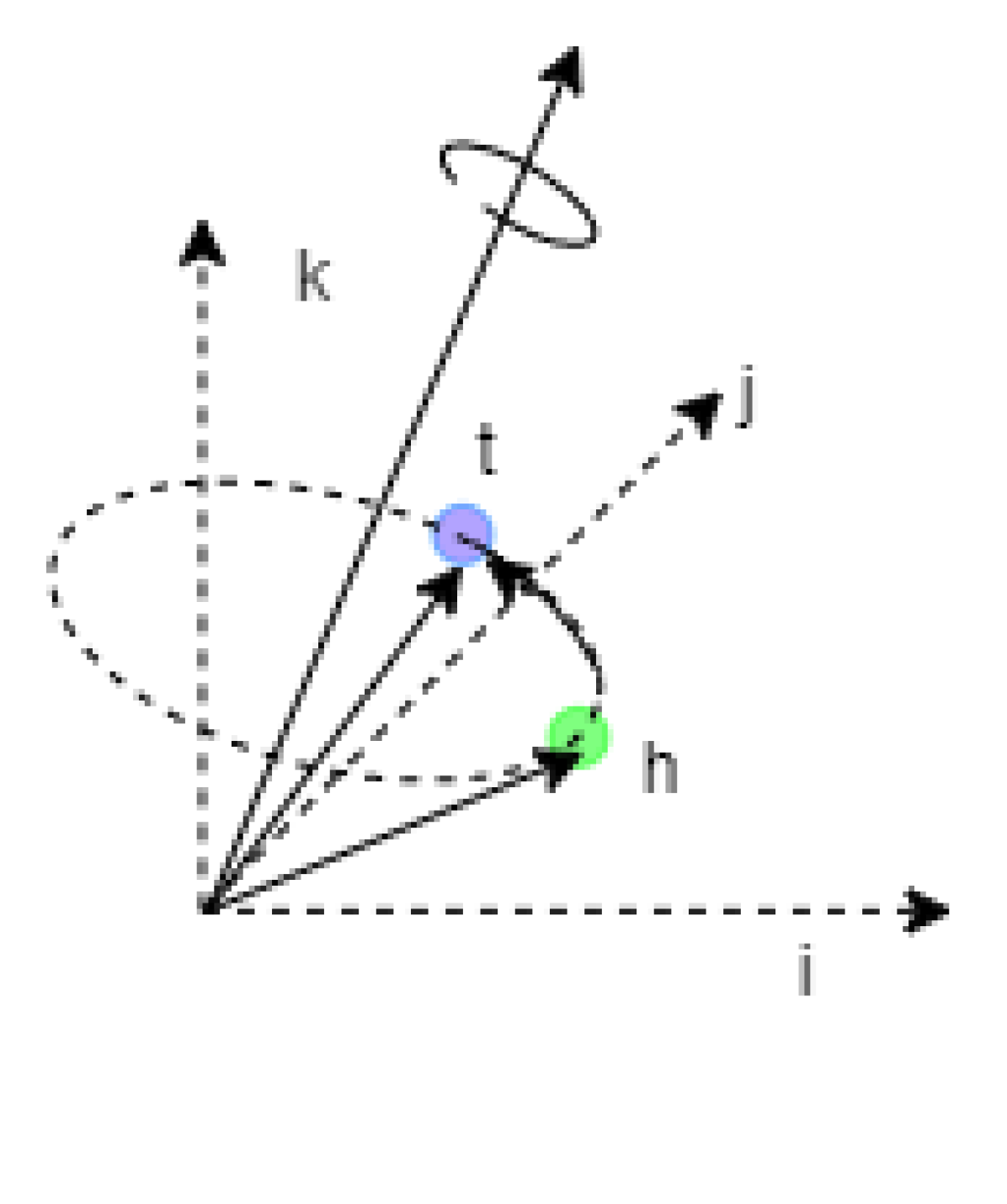
(a) NagE

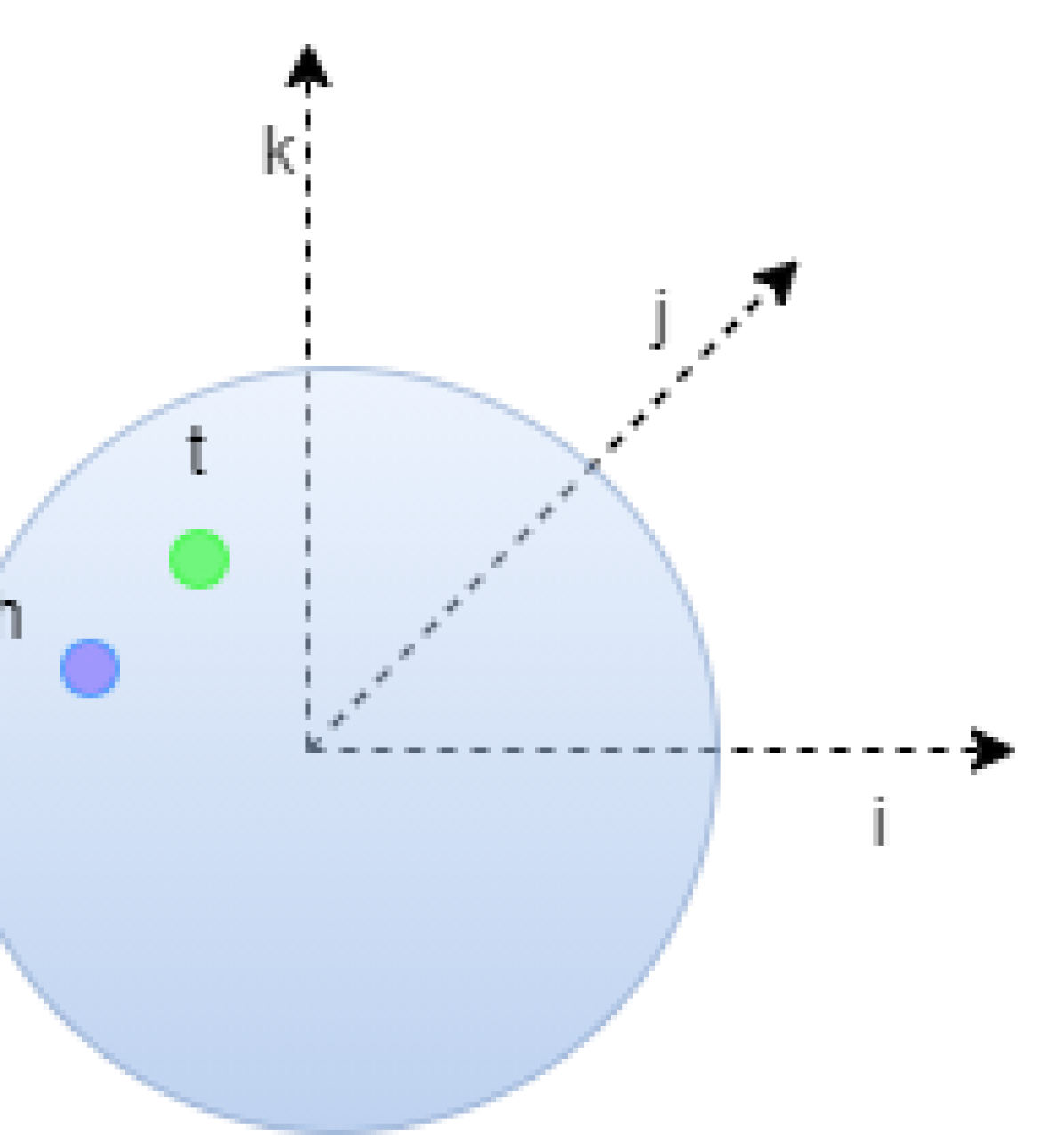
(b) QuatE

(c) HopfE step 1: Rotation

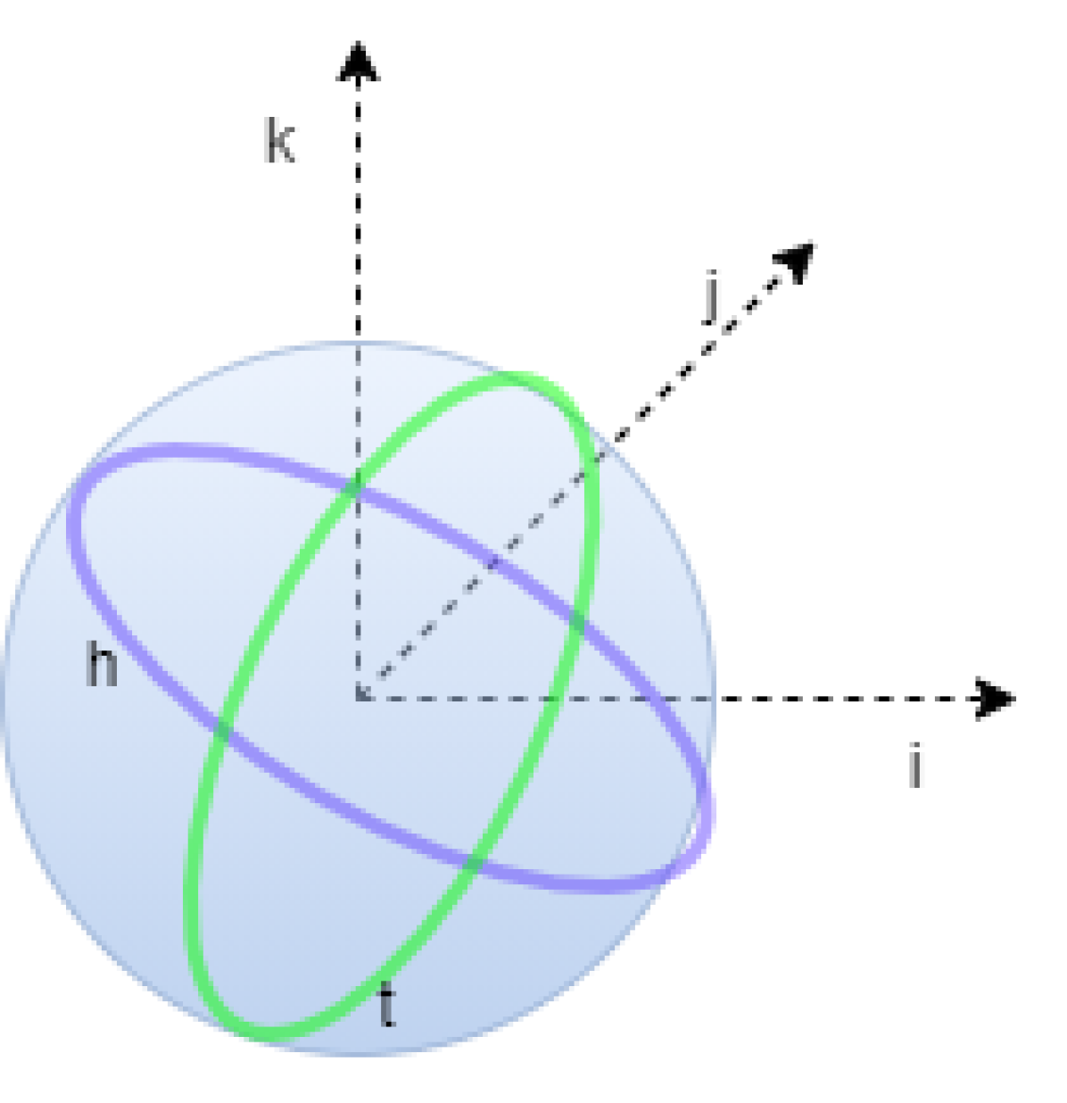
(d) HopfE step 2: Fibration

Figure 1. For a given triple ¡h,r,t¿ in three-dimensions (i,j,k); NagE provides geometric interpretability by rotating the entities in a 3D space (Figure (a)). Conversely, QuatE (Figure (b)) achieves higher order expressiveness by transforming the entities using the relational quaternion in 4D space, although it loses geometric interpretability. Here, the entities are stereo-graphically projected on a 3D sphere for understanding. HopfE first performs a rotation in 3D followed by a fibration to 4D as shown in Figures (c) and (d). This allows retaining geometric interpretability in 4D as entities are now depicted as fibers. In Figure (d), the stereo-graphic projection of two fibrations is shown before performing the rotations.

Publicly available Knowledge Graphs (KGs) (e.g., Freebase (Bollacker et al., 2007) and Wikidata (Vrandecic, 2012)) expose interlinked representation of structured knowledge for several information extraction tasks such as entity linking, relation extraction, and question answering (Bastos et al., 2021; Sakor et al., 2020; Lu et al., 2019). However, publishing ever-growing KGs is often confronted with incompleteness, inconsistency, and inaccuracy (Ji et al., 2016). Knowledge Graph Embeddings (KGE) methods have been proposed to overcome these challenges by learning entity and relation representations (i.e., embeddings) in vector spaces by capturing latent structures in the data (Wang et al., 2014). A typical KGE approach follows a two-step process (Gesese et al., 2019; Wang et al., 2017): 1) determining the form of entity and relation representations, 2) use a transformation function to learn entity and relation representations in a vector space for calculating the plausibility of KG triples via a scoring function. Intuitively, KGE approaches consider a set of original ”connectivity patterns” in the KGs and learn representations that are approximately able to reason over the given patterns (expressiveness property of a KGE model (Wang et al., 2018)). For example, in a connectivity pattern such as symmetric relations (e.g. sibling), anti-symmetric (e.g., father), inverse relations (e.g., husband and wife), or compositional relations (e.g., mother’s brother is uncle); expressiveness means to hold these patterns in a vector space.

Limitations of state-of-the-art KGE Models: KGs are openly available, and in addition they are largely explainable because of the explicit semantics and structure (e.g., direct and labeled relationships between neighboring entities). In contrast, KG embeddings are often referred to as sub-symbolic representation since they illustrate elements in the vector space, losing the original interpretability deduced from logic or geometric interpretations (PALMONARI and MINERVINI, 2020). Similar issue has been observed in a few initial KGE methods (Bordes et al., 2013; Wang et al., 2014; Lin et al., 2015) that lack interpretability, i.e., these models fail to link the connectivity patterns to a geometric interpretation such as rotation (Sun et al., 2018). For example, in inverse relations, the angle of rotation is negative; in composition, the rotation angle is an addition ($r_{1}+r_{2}=r_{3}$), etc. Other KGE approaches such as RotatE (Sun et al., 2018) and NagE (Yang et al., 2020) provide interpretability by introducing rotations in two-dimensional (2D) and three-dimensional (3D) spaces respectively, to preserve the connectivity patterns. Conversely, QuatE (Zhang et al., 2019) imposes a transformation on the entity representations by quaternion multiplication with the relation representation. QuatE aims for higher dimensional expressiveness by performing entity and relational transformation in hypercomplex space (4D in this case) (Zhang et al., 2019). Quaternions enable expressive modeling in four-dimensional space and have more degree of freedom than transformation in complex plane (Zhang et al., 2019; Zhu et al., 2018; Zhang et al., 2020b). Albeit expressive and empirically powerful, QuatE fails to provide explicit and understandable geometric interpretations due to its dependency on unit quaternion-based transformation (Yang et al., 2020; Lu and Hu, 2020). Hence, it is an open research question as to how can a KGE approach maintain the geometric interpretability and simultaneously achieves the model’s expressiveness in four-dimensional space?

Proposed Hypothesis: The essential research gap to achieve interpretability in four-dimensional space for a KGE embedding motivates our work. QuatE transforms one point (i.e., entity representation) to another in the 4D hypersphere $S^{3}$ (Zhang et al., 2019). Unlike QuatE, we hypothesize that it is viable to map a three-dimensional point to a circle in the four-dimensional space. Our rationale for the choices are: 1) the relational rotations in 3D sphere $S^{2}$ are already proven to be interpretable (i.e., (Yang et al., 2020; Gao et al., 2020)). However, transformations as done in QuatE lack geometric interpretability (Lu and Hu, 2020). Hence, performing relation rotations in $S^{2}$ will allow us to inherit these proven interpretable properties. 2) Mapping the entity representation of $S^{2}$ to a circle in a higher dimension can illustrate these representations as fibers (Whitney, 1940) (i.e., manifolds) for maintaining geometric interpretations while providing the expressiveness of 4D embeddings (cf., Figure 1). In other words, by representing entities as fibers, we can aim for a direct mapping between rotations in $S^{2}$ to transformation of fibers in the $S^{3}$, without compromising interpretability in four-dimensional space. 3) By converting a point of $S^{2}$ to a circle in $S^{3}$, we aim to semantically enrich entity embeddings through KG ontology (entity-aliases, entity-types, descriptions, and entity-labels as textual literals (Gesese et al., 2019)) onto the points on the fiber.

Approach: In this paper, we present HopfE- a novel KGE approach aiming to increase the expressiveness in higher dimensional space while maintaining the geometric interpretability (Figure 1). Specifically, in HopfE, we first rotate the relational embeddings in the 3D Euclidean space using Quaternion (Vicci, 2001) rotations. In the next step, the point (i.e., entity representation) in the 3D sphere is converted to a circle on the 4D hypersphere using inverse Hopf Fibration (Hopf, 1931). We propose to use the extra dimension gained by Hopf mapping to also represent the entity attributes for semantically enriching the embeddings.
Contributions. The key contributions of this work are: 1) Our work (theoretically and empirically) legitimizes Hopf Fibration’s application in KG embeddings. To the best of our knowledge, we are the first to incorporate Hopf Fibration mapping for any representation learning approach. 2) We bridge the important gap between geometric interpretability and four-dimensional expressiveness of a knowledge graph embedding method. 3) We provide a way to induce entity semantics in 4D, keeping the rotational interpretability intact. 4) Our empirical results achieves comparable state-of-the-art performance on four well-known KG completion datasets.

The structure of the paper is follows: Section 2 reviews the related work. Section 3 formalizes the problem. Section 4 describes theoretical foundations and Section 5 describes our proposed approach. Section 6 describes experiment setup. Our results are discussed in Section 7. We conclude in Section 8.

2. Related Work

Considering KGE is an extensively studied topic in the literature (Allen et al., 2021; Zhao et al., 2020b; Ji et al., 2021; Chami et al., 2020; Gao et al., 2020), we stick to the work closely related to our approach. Previous works on KG embeddings are primarily divided into translation and semantic matching models (Wang et al., 2017). Translational models use distance-based scoring functions which are often based on learning a translation from the head entity to the tail entity. The first translation-based approach was TransE (Bordes et al., 2013) which models the composition of the entities and relations as $e_{1}+r=e_{2}$. The second category (i.e., semantic matching) uses similarity-based scoring functions. The basic idea is to measure the plausibility of KG triples by matching the latent semantics of entities and relations expressed in their vector space representations. Distmult (Yang et al., 2015) is a semantic matching model where the entities are represented as vectors. The relations are diagonal matrices, and the composition is a bilinear product of the entities and relations. ComplEx (Trouillon et al., 2016) is a modification of DistMult where the parameters are in the complex space. RotatE (Sun et al., 2018) was the first to propose the translation as a rotation of the entities in the complex plane for geometric interpretability. RotatE models the rotation in the 2D plane and has symmetric, antisymmetric, composition, and inversion properties. This rotation, however, induces a strict compositional dependence between the relations. Yang et al. (Yang et al., 2020) introduced NagE, that provides a group theoretic perspective of rotations similar to RotatE by using Non-Abelian ($SO(3)$ and $SU2E$) groups. These groups give a geometrical interpretation of rotations in 3D, and being non-commutative groups, they solve the problem of strict compositionality. QuatE (Zhang et al., 2019) has modeled the relational rotations in the quaternion four-dimensional space, thus making the model more expressive. QuatE also studied that increasing spatial dimensions such as to Octonion does not increase performance compared to modeling relation and entities in 4D. We position our work at the intersection of QuatE, and NagE approaches (cf. Figure 1). In contrast with QuatE that does transformation using quaternion multiplication, we perform $SO(3)$ rotations using quaternion relation to inherit the geometric interpretability of NagE. The inverse Hopf Fibration lets us perform the dimensional mapping which has found applications in diverse domains such as rigid body mechanics (Marsden and Ratiu, 1995) and quantum information theory (Mosseri and Dandoloff, 2001). Furthermore, there are extensive works for inducing schema and ontology information in the embedding models such as entity types (Zhao et al., 2020a; Lin et al., 2016), entity descriptions (Wang et al., 2016), and literals (Gesese et al., 2019). We also aim to induce entity semantic properties (textual literals) into HopfE. Unlike existing methods (Gesese et al., 2019), that concatenate the semantic and latent embeddings, we would like to look at the latent space for representing entity attributes.

3. Problem Formulation

We define a KG as a tuple $KG=(\mathcal{E},\mathcal{R},\mathcal{T}^{+})$ where $\mathcal{E}$ denotes the set of entities (vertices), $\mathcal{R}$ is the set of relations (edges), and $\mathcal{T}^{+}\subseteq\mathcal{E}\times\mathcal{R}\times\mathcal{E}$ is a set of all triples. A triple $\uptau=(e_{h},r_{ht},e_{t})\in\mathcal{T}^{+}$ indicates that, for the relation $r_{ht}\in\mathcal{R}$, $e_{h}$ is the head entity (origin of the relation) while $e_{t}$ is the tail entity. Since $KG$ is a multigraph; $e_{h}=e_{t}$ may hold and $|\{r_{e_{h},e_{t}}\}|\geq 0$ for any two entities. We define the tuple $(A^{e},\tau^{e})=\varphi(e)$ obtained from a context retrieval function $\varphi$, that returns, for any given entity $e$, the set: $A^{e}$ which is a set of all attributes of the entity such as aliases, descriptions, and type. $\tau^{e}\subset\mathcal{T}^{+}$ is the set of all triples with head at $e$. The KB completion task (KBC) predicts the entity pairs $\langle e_{i},e_{j}\rangle$ in the Knowledge Graph that have a relation $r_{ij}\in\mathcal{R}$ between them. Similar to other researchers (Zhang et al., 2019; Yang et al., 2020), we view KBC as a ranking task. In addition, we also aim to model KG contextual information to improve the ranking.

4. Theoretical Foundations

4.1. Quaternions and Rotations in 3D

Quaternions (Hamilton, 1844) are a numerical representation of vectors in four dimensions. It can be considered as an ordered tuple $(a,b,c,d)$ of numbers represented by $a+bi+cj+dk$ where $a$ is the real component and $b,c,d$ are the imaginary components. The norm (Pugh and Pugh, 2002) of the quaternion $a+bi+cj+dk$ can be represented by $\sqrt{a^{2}+b^{2}+c^{2}+d^{2}}$. From hereon, ”$*$” is multiplication operation, ”$\odot$” is an element-wise product, ”$\otimes$” denotes Hamilton product. In the following, we describe the details of rotation in 3D sphere.

Theorem 4.1.

For a pure quaternion $v=p_{1}i+p_{2}j+p_{3}k$ in 3D that has real components as zero, the quaternion $r=a+bi+cj+dk$ with unit norm gives a rotational map $rvr^{-1}$, where the axis of rotation denoted by bi+cj+dk, and the angle of rotation by $2\arccos{a}$

Proof.

We divide the proof into three sections where we prove that the norm of $v$ is preserved, where $(b,c,d)$ is the eigen vector of the rotational map, and the angle of rotation can be given in terms of $a$. The rotational map $R_{r}(v)=rvr^{-1}$ has the norm $\left\lVert R_{r}(v)\right\rVert=\left\lVert rvr^{-1}\right\rVert=\left\lVert r\right\rVert*\left\lVert v\right\rVert*\left\lVert r^{-1}\right\rVert$. We have assumed $r$ to have unit norm, it’s inverse will also have unit norm. Hence, the norm of $v$ is maintained. To prove that $b,c,d$ is the eigen vector of the rotational map, it is sufficient to show that the rotation of $bi+cj+dk$ under the rotation map results in a scaled version of the vector:

$$R_{r}(bi+cj+dk) =(a+bi+cj+dk)\otimes$$

$$(bi+cj+dk)\otimes\frac{(a-bi-cj-dk)}{a^{2}+b^{2}+c^{2}+d^{2}}$$

$$=bi+cj+dk$$

Hence we obtain the same vector with scaling operation. Now we prove that the angle of rotation can be given in terms of $a$. We can consider $a$ vector perpendicular to the axis vector $bi+cj+dk$. Let $w=ci-bj$ be this vector without loss of generality. Then, it’s rotation is given by:

$$R_{r}(w) =(a+bi+cj+dk)\otimes(ci-bj)$$

$$\otimes(a-bi-cj-dk)$$

$$=((ac+db)i+(-ab+dc)j-(b^{2}+c^{2})k)$$

$$\otimes(a-bi-cj-dk)$$

$$=(c*(a^{2}-b^{2}-c^{2}-d^{2})+2adb)i+$$

$$(-b*(a^{2}-b^{2}-c^{2}-d^{2})+2adc)j+(-2ab^{2}-2ac^{2})k$$

The cosine of the angle between w and $R_{r}(w)$ is given by

$$\cos{\theta} =\frac{w.R_{r}(w)}{\lVert w\lVert^{2}}$$

$$=a^{2}-b^{2}-c^{2}-d^{2}=2a^{2}-1$$

$$\theta =2\arccos{a}$$

If $b=c=0$, we take $w=i$ to get the same result. Thus, the rotational map $a+bi+cj+dk$ encodes the axis and angle of rotation. ∎

4.2. Hopf Fibration

Two spaces are said to be homotopic if there exists a set of continuous deformations from one space to another (Baues and Baues, 1989). For example, a solid circular disc is homotopic to a point as it could be deformed along the radial lines to a point.

Definition 4.2 (Homotopy Lifting).

Given a map $\pi:E\xrightarrow[]{}B$ between two topological spaces $E$ and $B$ and a topological space $X$, we say that $\pi$ has a homotopy lifting property with respect to $X$ if for a homotopy $g:X\times[0,1]\xrightarrow[]{}B$, there exists a homotopy $f:X\times[0,1]\xrightarrow[]{}E$ such that $\pi\circ f=g$.

Definition 4.3 (Fibration).

A fibration is a map $f:E\xrightarrow[]{}B$ between two topological spaces $E$ and $B$ such that the homotopy lifting property is satisfied for all spaces.

First introduced in 1931, Hopf Fibration is a mapping from $S^{3}$ to $S^{2}$ (Hopf, 1931; Lyons, 2003). For the quaternion $r=a+bi+cj+dk$ this map is given by

(1) $$M(r)=(a^{2}+b^{2}-c^{2}-d^{2},2(ad+bc),2(bd-ac))$$

This is equivalent to applying the rotational map $R_{r}$ to the point (1,0,0). The Hopf map ($M(r)$) assigns all $r$ in $S^{3}$ to $P$ in $S^{2}$, such that $R_{r}$ would rotate $(1,0,0)$ to $P$. We could also verify that multiplying $e^{it}=cos(t)+i*sin(t)$ to this map doesn’t change the rotation. The inverse Hopf map gives the pre-image of point $P$ by:

Lemma 4.0.

For a point $P=(p1,p2,p3)$ the inverse Hopf map is given by $M^{-1}(P)=r^{\prime}e^{it}$ where $0\leq t\leq 2\pi$ and $r^{\prime}$ can be given by one of the below equations:

(2) $$r^{\prime}=\frac{1}{\sqrt{2(1+p_{1})}}((1+p_{1})i+p_{2}j+p_{3}k)$$

OR

(3) $$r^{\prime}=\frac{\sqrt{1+p_{1}}}{2}*(1-\frac{p_{3}i}{1+p_{1}}+\frac{p_{2}k}{1+p_{1}})$$

Proof.

We begin by noting that (from Theorem 4.1),

$$M(r^{\prime}e^{it})=(r^{\prime}e^{it})\otimes i\otimes(r^{\prime}e^{it})^{-1}$$

Substituting for $r^{\prime}e^{it}$ from Equation 2 we get,

$$r^{\prime}\otimes e^{it} =\frac{1}{\sqrt{2(1+p_{1})}}((1+p_{1})i+p_{2}j+p_{3}k)\otimes$$

$$(\cos{t}+i*\sin{t}))$$

$$=\frac{1}{\sqrt{2(1+p_{1})}}*(\sin{t}*(1+p_{1})+$$

$$\cos{t}*(1+p_{1}))i+(p_{2}*\cos{t}+p_{3}*\sin{t})j+$$

$$(p_{3}*\cos{t}-p_{2}*\sin{t})k)$$

Similarly we get the compliment $\overline{r^{\prime}e^{it}}$ as,

$$\overline{r^{\prime}\otimes e^{it}} =\frac{1}{\sqrt{2(1+p_{1})}}*(\sin{t}*(1+p_{1})$$

$$-\cos{t}*(1+p_{1}))i-(p_{2}*\cos{t}+p_{3}*\sin{t})j+$$

$$-(p_{3}*\cos{t}-p_{2}*\sin{t})k)$$

The Hopf Map of the set of points on $r^{\prime}\otimes e^{it}$ is the point in $S^{2}$ that is obtained by rotation of $(1,0,0)$ using any of these quaternions,

$$M(r^{\prime}e^{it}) =(r^{\prime}e^{i}t)\otimes(i)\otimes(\overline{r^{\prime}e^{i}t})$$

$$=p_{1}i+p_{2}j+p_{3}k=P$$

therefore, $M^{-1}{(P)}=r^{\prime}e^{it}$. (also applicable to Equation 3). ∎

A point on the 3D sphere is mapped to a circle by the Equation 2. Furthermore, a set of points is mapped to a group of linked rings, and a circle in $S^{2}$ is mapped to a torus in $S^{3}$ as can be seen in the Figure 2. The property of linked circles is stated in Lemma 4.5.

Lemma 4.0.

Every pair of fiber formed by the Hopf Map are linked to each other forming a set of linked circles.

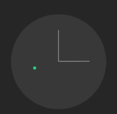
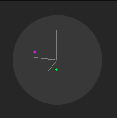
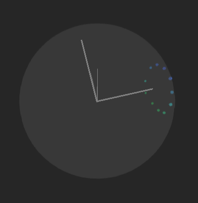
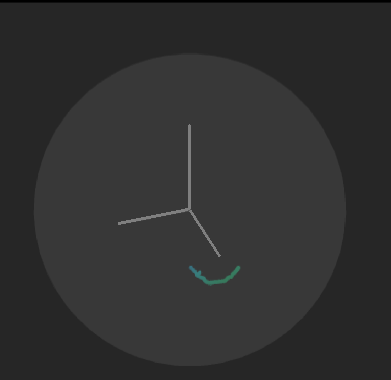
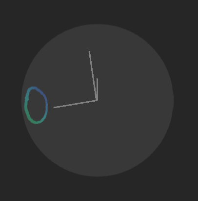
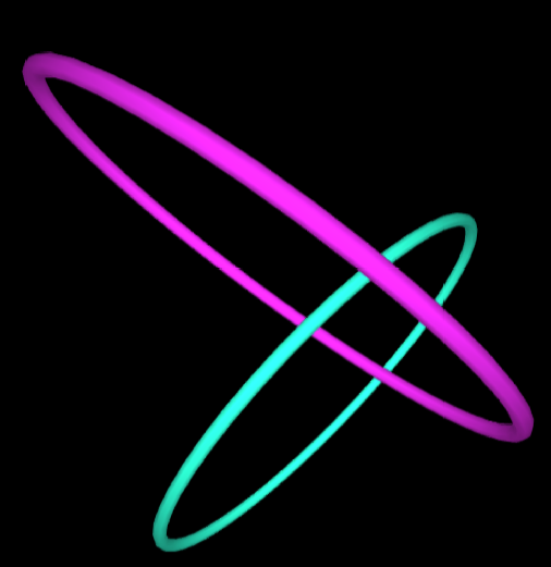
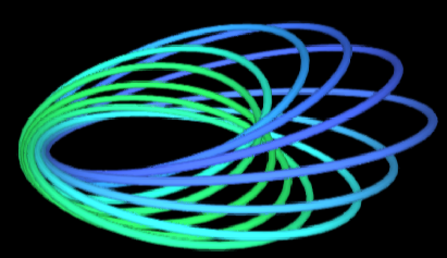
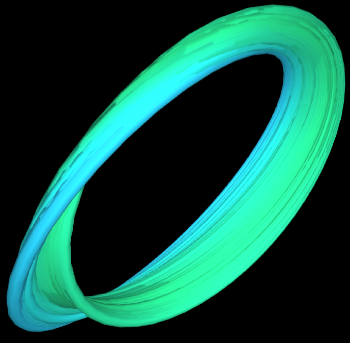
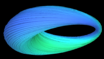
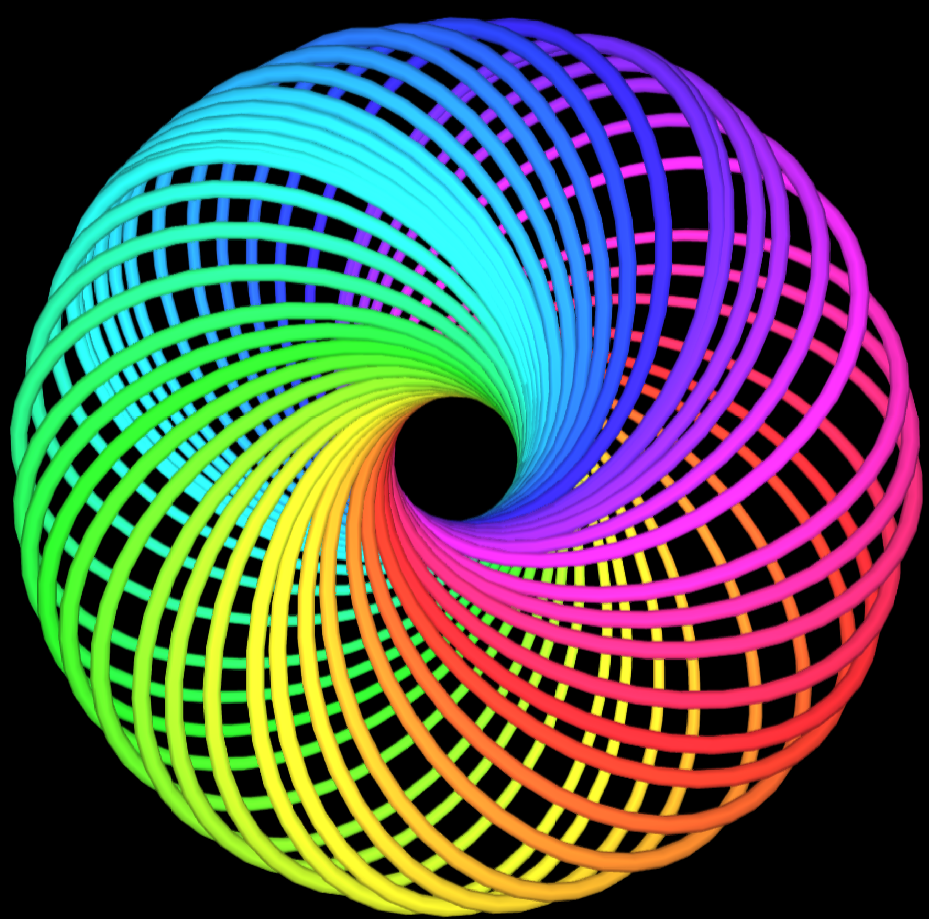
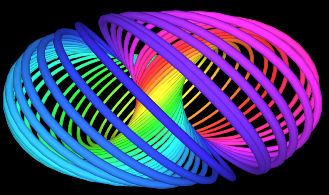
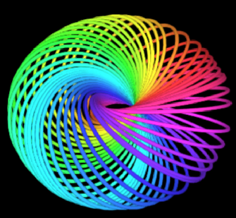
Figure 2. We show the Hopf fibers of points on $S^{2}$ visualized (Li, NA) using the stereo-graphic projection from $S^{3}$ to $S^{2}$. The first row from the top illustrates (left to right): a point, two points, discrete points, arc, and circle in 3D space. The second row (left to right) illustrates the stereographic projection of corresponding fibers in 3D. The third row (left to right) shows the set of points on the grid circle of $S^{2}$ and its corresponding top-view, side-view, and isometric views, respectively.

4.3. Optimal Transport

The aim of optimal transport (Monge, 1781) is to minimize the cost of transport from one (probability) measure to another. The well known Wasserstein Distance (Villani, 2008) defines the optimal transport plan to move an amount of matter from one location to another. We rely on the principle of optimal transport considering we aim to map entity representation from one plane to another hyperplane.

Definition 4.6.

Let $p\in[1,\infty)$ and c: $R^{n}\times R^{n}$ $\xrightarrow{}[0,\infty)$ be the cost of transporting the measure $\mu$ to $\nu$, then the $p^{th}$ Wasserstein distance between the measures is given by

(4) $$W_{p}(\mu,\nu)=\inf_{\gamma\in\Pi(\mu,\nu)}\left(\int_{R^{n}\times R^{n}}c(x,y)^{p}\partial{\gamma}\right)^{\frac{1}{p}}$$

where $\Pi$ is the transport plan between the measures $\mu$ and $\nu$.

Theorem 4.7.

The minimum of the euclidean distance between the points of the Hopf fibers of two points in the $\delta$ vicinity in $S^{2}$ is bounded from above by $\delta^{2}$.

Proof.

Consider a point $P=(p_{1},p_{2},p_{3})$ in $S^{2}$ and another point $P^{{}^{\prime}}=(p_{1}^{{}^{\prime}},p_{2}^{{}^{\prime}},p_{3}^{{}^{\prime}})$ such that

$$\lVert P-P^{{}^{\prime}}\rVert=\delta$$

From Lemma 4.4 we know that the the fiber of $P$ is given by

$$\frac{1}{\sqrt{2(1+p_{1})}}((1+p_{1})i+p_{2}j+p_{3}k)\otimes e^{it}$$

and the fiber of $P^{{}^{\prime}}$ is given by

$$\frac{1}{\sqrt{2(1+p_{1}^{{}^{\prime}})}}((1+p_{1}^{{}^{\prime}})i+p_{2}^{{}^{\prime}}j+p_{3}^{{}^{\prime}}k)\otimes e^{it^{{}^{\prime}}}$$

, where $t$ and $t^{{}^{\prime}}$ are the respective parameters. The square of the euclidean distance ($D$) between any two points of the fibers is given by the $l_{2}$ norm as below

$$D =(-k*\sin(t)(1+p_{1})+k^{{}^{\prime}}sin(t^{{}^{\prime}})(a+p_{1}^{{}^{\prime}}))^{2}$$

$$=(k*\cos(t)(1+p_{1})-k^{{}^{\prime}}sin(t^{{}^{\prime}})(a+p_{1}^{{}^{\prime}}))^{2}$$

$$=(k*(\cos(t)p_{2}+\sin(t)p_{3})-k^{{}^{\prime}}(cos(t^{{}^{\prime}})p_{2}^{{}^{\prime}}+sin(t^{{}^{\prime}})p_{3}^{{}^{\prime}}))^{2}$$

$$=(k*(\cos(t)p_{3}-\sin(t)p_{2})-k^{{}^{\prime}}(cos(t^{{}^{\prime}})p_{3}^{{}^{\prime}}+sin(t^{{}^{\prime}})p_{2}^{{}^{\prime}}))^{2}$$

We then proceed by taking the derivative of $D$ with respect to $t$ and $t^{{}^{\prime}}$, equating them with $0$ for the optimal solution. Then, we have

$$\frac{\partial{f}}{\partial{t}}=0,\frac{\partial{f}}{\partial{t^{{}^{\prime}}}}=0$$

Solving for $t$ and $t^{{}^{\prime}}$ at $\delta\approx 0$, gives

$$t=\frac{\delta p_{1}(p_{3}-p_{2})}{(1+p_{1})(p_{3}^{2}+p_{2}^{2})},t^{{}^{\prime}}=\frac{\delta(p_{3}-p_{2})}{(1+p_{1})(p_{3}^{2}+p_{2}^{2})}$$

Substituting these values in $D$ we get $D\leq\mathcal{O}(\delta^{2})$. ∎

From Theorem 4.7 we can deduce that the minimum distance between the fibers is a monotone increasing function of the distance between their corresponding points. Therefore:

Corollary 4.0.

For any set of entities, if there is a configuration satisfying the relations between them in $S^{2}$- then there will also be a configuration on the fibers that satisfy the concerning relations.

Hence, from Corollary 4.8, the triples expressed in the lower dimension are the same as in the higher dimension after the mapping. Now we want to show that the higher dimensional space can represent more triples. We state the corresponding Lemma:

Lemma 4.0.

The triple set represented by rotations in $S^{2}$ is not equal to the set of triples that can be represented in $S^{3}$ after the fibration.

Proof.

Let $\tau^{2}$ be the set of triples that can be represented in $S^{2}$ and $\tau^{3}$ be the set of triples that can be expressed in $S^{3}$ after the Fibration(mapping). We have to show that $\tau^{2}\nsubseteq\tau^{3}$. For this, it is enough to show that even a single configuration of triples in $\tau^{3}$ is not in $\tau^{2}$. Consider three entities $e_{1}$, $e_{2}$ and $e_{3}$ with relation $r_{1}$ existing between them such that ${(e_{1},r_{1},e_{2}),(e_{2},r_{1},e_{3}),(e_{1},r,e_{3})}\in\tau^{+}$ and ${(e_{3},r_{1},e_{2}),(e_{2},r_{1},e_{1}),(e_{3},r_{1},e_{1})}\in\tau^{-}$ where $\tau^{+}$ and $\tau^{-}$ are the set of positive and negative triples respectively. Let $E_{1},E_{2},E_{3}\in R^{3}$ be the representations of these entities in $S^{2}$ and let $R_{1}\in H$ ($H$ is Hamiltonian Space) be the relation quaternion. Thus we have,

$R_{1}\otimes E_{1}\otimes R_{1}^{-1}=E_{2};R_{1}\otimes E_{2}\otimes R_{1}^{-1}=E_{3};R_{1}\otimes E_{1}\otimes R_{1}^{-1}=E_{3}$

This implies that $E_{1}=E_{2}=E_{3}$ and the axis of rotation is along these vectors. However, then we would also have:

$R_{1}\otimes E_{2}\otimes R_{1}^{-1}=E_{1};R_{1}\otimes E_{3}\otimes R_{1}^{-1}=E_{2};R_{1}\otimes E_{3}\otimes R_{1}^{-1}=E_{1}$

which is a contradiction, so the relational operator in $S^{2}$ cannot represent the triples’ set. In $S^{3}$, we have each of these entities’ fibers coinciding with each other from the above analysis. We could now select $A_{1}^{1},A_{1}^{2}\in C$, $A_{2}^{1},A_{2}^{2}\in C$ and $A_{3}^{1}\in C$ as the attributes for $e_{1}$, $e_{2}$ and $e_{3}$ respectively. We define $R^{c}(\in C)=e^{i\theta}$ to be the rotational operator in the complex plane $C$ for the relation. Setting $A_{1}^{1}=e^{i\theta_{1}}$, $A_{1}^{2}=A_{2}^{1}=e^{i\theta_{2}}$ and $A_{2}^{2}=A_{3}^{1}=e^{i\theta_{3}}$, where $\theta_{2}-\theta_{1}=\theta_{3}-\theta_{2}=\theta$, we can see that the set of triples (both positive and negative) can be represented by the mapping in $S^{3}$. ∎

Theorem 4.10.

The set of triples that can be represented by rotations in $S^{2}$ is a strict subset of the set of triples that can be represented in $S^{3}$ after the fibration.

Proof.

Let $\tau^{2}$ be the set of triples that can be represented in $S^{2}$ and $\tau^{3}$ be the set of triples that can be expressed in $S^{3}$ after the fibration(mapping). We have to show that $\tau^{2}\subset\tau^{3}$. From 4.8 we have $\tau^{2}\subseteq\tau^{3}$ and from 4.9 we have $\tau^{2}\nsubseteq\tau^{3}$. Thus, we can deduce that $\tau^{2}\subset\tau^{3}$ and hence the proof. ∎

5. Our Approach

5.1. Modeling rotations using Quaternions

As noted in the Theorem 4.1, the unit quaternion is isomorphic to the $SU(2)$ group which in turn is homomorphic to the $SO(3)$ rotation group (also observed by NagE (Yang et al., 2020)). This allows us to use the quaternion for rotations in the 3D Euclidean space as below:

(5) $$w^{{}^{\prime}}=q\otimes w\otimes\overline{q}$$

where $q$ is the quaternion, $\overline{q}$ is the inverse of $q$, $w$ is the vector in 3D space and $w^{{}^{\prime}}$ is the rotated vector. In other words, $q$ is the dimension-wise relation quaternion, $w$ is the dimension-wise entity representation in 3D space, and $w^{{}^{\prime}}$ is the rotated entity representation in the same space. If $q=a+bi+cj+dk$ then $\overline{q}=\frac{a-bi-cj-dk}{\sqrt{a^{2}+b^{2}+c^{2}+d^{2}}}$.

Reusing $SO(3)$ rotations from NagE in this step helps us inherit its geometric for the completion of our approach.

Model	Scoring function	Parameters	$\mathcal{O}_{time}$
TransE (Bordes et al., 2013)	$\lVert E_{h}+W_{r}-E_{t}\rVert$	$E_{h},W_{r},E_{t}\in R^{k}$	$\mathcal{O}(k)$
DistMult (Yang et al., 2015)	$\langle W_{r},E_{h},E_{t}\rangle$	$E_{h},W_{r},E_{t}\in R^{k}$	$\mathcal{O}(k)$
ComplEx (Trouillon et al., 2016)	$Re(\langle W_{r},E_{h},\overline{E_{t}}\rangle)$	$E_{h},W_{r},E_{t}\in C^{k}$	$\mathcal{O}(k)$
RotatE (Sun et al., 2018)	$\lVert E_{h}\odot Wr-E_{t}\rVert$	$E_{h},W_{r},E_{t}\in C^{k},\mid W_{r}\mid=1$	$\mathcal{O}(k)$
QuatE (Zhang et al., 2019)	$E_{h}\otimes W_{r}\cdot E_{t}$	$E_{h},W_{r},E_{t}\in H^{k}$	$\mathcal{O}(k)$
HopfE (ours)	$\lVert M(W_{r}\otimes E_{h}\otimes\overline{W_{r}},A^{h})-M(E_{t},A^{t})\rVert$	$E_{h},E_{t}\in(R^{3})^{k},W_{r}\in H^{k},A^{h},A^{t}\in C^{k}$	$\mathcal{O}(k)$

Table 1. KGE Overview. $W_{r}$ is the relation representation, $E_{h}$, $E_{t}$ are the entity representations, $M$ is the inverse Hopf map.

5.2. Homotopy Lifting using Inverse Hopf Map

In this step, we aim to achieve expressiveness in higher dimension space, i.e., 4D hypersphere as our main contribution. The inverse map with the equations described in Lemma 4.4 lifts the point (rotated entity representation from Equation 5) in $S^{2}$ to a set of points (i.e., fiber) lying in a higher-dimensional space. Once both entities are mapped as individual fibers in the 4D hypersphere, it is possible to ground connectivity patterns in rotations as done by NagE and RotatE in the lower dimensional spaces. Each point on the fiber has the same geometric property for a given entity. We parametrize the entities to fix the location of these sets of points on the fiber. Hence, we now have a bunch of points on the fiber for each entity, which could represent the entity’s semantic attributes. Formally we define a set of parameters $t$ for each entity corresponding to its semantic attribute $A^{e}$ (cf., section 3). These parameters could be used to find the set of points on the fiber as below:

(6) $$e_{i}=r^{\prime}\otimes(\cos(t)+\sin(t)i)$$

where $e_{i}$ is the entity quaternion per dimension and $r^{\prime}$ is obtained from either Equations 2 or 3. From Corollary 4.8, we obtain that the equation 6, which takes the representation to a higher dimension, does not cause a loss in expressivity.

Claim 5.1.

Translation methods, in the euclidean space, require at least $n-1$ dimensions to model an n-clique relational pattern between $n$ entities.

A direct consequence of Claim 5.1 is that to model dense relations; we would need a dimension proportionate to the number of entities. We propose an increase in the model expressivity by increasing the entity attribute size while keeping the dimensions same. The entity attribute size (i.e. number of heads) is $\mid A^{e}\mid$. While increasing the number of heads will make the model more expressive, it may also increasing the training latency. In ablation results, we aim to study the relation between model expressivity and the attribute heads for a fixed time interval (cf., section 4).

5.3. Inducing Semantics

Once the point is mapped to the fiber using inverse Hopf Fibration, we propose to learn a set of points that would inform about the various semantics/attributes of the entity. One possible way for the operation would be to have the points spread out on the circle (fiber) based on the semantic attributes of the entity. Taking inspiration from (Gesese et al., 2019; Zhao et al., 2020a) we use the textual literals widely available for an entity in the standard KGs namely: entity description, Instance of (type of entity such as human), Alias (alternative names) and Surface forms (label of the entity). Specifically we use the CBOW model (Mikolov et al., 2013) to aggregate the embeddings of the tokens in each semantic attribute. These embeddings could be initialized from a standard model such as Glove (Pennington et al., 2014). The parameter $t$ in Equation 6 is learned from the semantics. We also tried with other methods such as initializing the parameters with the semantic embeddings and using an MLP to learn the final representation after concatenating the structural and semantic embeddings, which does not perform better.

Model	WN18					WN18RR
	MR	MRR	Hits@1	Hits@3	Hits@10	MR	MRR	Hits@1	Hits@3	Hits@10
TransE (Bordes et al., 2013)	-	0.495	0.113	0.888	0.943	3384	0.226	-	-	0.501
DistMult (Yang et al., 2015)	655	0.797	-	-	0.946	5110	0.43	0.39	0.44	0.49
ComplEx (Trouillon et al., 2016)	-	0.941	0.936	0.945	0.947	5261	0.44	0.41	0.46	0.51
RotatE (Sun et al., 2018)	309	0.949	0.944	0.952	0.959	3340	0.476	0.428	0.492	0.571
NagE (Yang et al., 2020)	-	0.950	0.944	0.953	0.960	-	0.477	0.432	0.493	0.574
QuatE (Zhang et al., 2019)	388	0.949	0.941	0.954	0.960	3472	0.481	0.436	0.500	0.564
HopfE	245	0.949	0.938	0.954	0.960	2885	0.472	0.413	0.500	0.586
HopfE + Semantics	99	0.945	0.934	0.951	0.961	2884	0.482	0.433	0.500	0.579

Table 2. Evaluation metrics on the WN18 and WN18RR datasets. Best results are in bold and second best is underlined.

5.4. Score function and Optimization Objective

In previous sections, we learned that lifting the dimensions of an entity would take us to the fiber (circle) in $S^{3}$. For two entities we would have two linked circles enriched with entity semantics. Now, we also need to find the distance between the attributes of two entities lying on the linked circles. This could be done, for example, by considering the corresponding attributes of the two entities or by taking a pairwise distance between the all combinations of the attributes. That would be computationally expensive. Hence, we propose another variant where we find an optimal matching between the attributes and then take the pairwise distance between these matched attributes. Table 1 provides an holistic overview of KGE details. To find an optimal matching between the set of entity attributes, we use the Wasserstein Distance using Equation 4. In practice, we have used the Sinkhorn iterations for faster computation of the Wasserstein distances (Cuturi, 2013). Let $\Pi$ be the optimal matching between the attributes $\emph{h}_{i}$ $\in$ $\emph{E}_{h}$ and $\emph{t}_{j}$ $\in$ $\emph{E}_{t}$ of an entity pair $h$ and $t$ respectively. The score function is:

(7) $$\small f_{r}(h,r_{ht},t)=\sum_{[i,j]\in\Pi}\frac{1}{2}\left(\lVert M(\mathcal{O}(\emph{h}_{i},r_{ht}))-M(\emph{t}_{j})\rVert+\lVert M(\mathcal{O}(\emph{t}_{j},\overline{r}))-M(\emph{h}_{i})\rVert\right)$$

where $\emph{h}_{i}$, $\emph{t}_{j}$ are the attributes (semantic properties) of the head and tail entities respectively, $r_{ht}$ is the relation. $\mathcal{O}$ represents the rotation operation on each dimension of the entity i.e. $\mathcal{O}(e_{d},r_{d})=r_{d}\otimes e_{d}\otimes\overline{r_{d}}$ where $r_{d}$ $\in$ $H$ and $e_{d}\in R^{3}$. Similarly, $M$ represents the inverse Hopf Map to the fiber in $S^{3}$, per dimension. In practice, for larger attribute sizes, computing the Wasserstein distance between a set of points could be computationally expensive. Therefore, we define its variant to consider the minimum distance between the two sets’ attributes. The score function transforms to:

(8) $$\small f_{r}(h,r_{ht},t)=\underset{\underset{\emph{t}_{j}\in\emph{E}_{t}}{\emph{h}_{i}\in\emph{E}_{h}}}{\inf}\frac{1}{2}\left(\lVert M(\mathcal{O}(\emph{h}_{i},r_{ht}))-M(\emph{t}_{j})\rVert+\lVert M(\mathcal{O}(\emph{t}_{j},\overline{r_{ht}}))-M(\emph{h}_{i})\rVert\right)$$

The loss function aims to minimize the score function for the positive triples and maximize it for the negative triples. More specifically, we use a self adverserial negative sampling loss similar to RotatE (Sun et al., 2018) as below:

$$\small L =\sum_{h,r_{ht},t\in\tau}-\log\left\{\sigma(\gamma+f_{r}(h,r_{ht},t))\right\}$$

$$- \sum_{h^{-},r_{ht},t^{-}\in\tau^{-}}p(h^{-},r_{ht},t^{-})\log\left\{\sigma(-(\gamma+f_{r}(h^{-},r_{ht}^{-},t^{-})))\right\}$$

where $\tau$ is the set of positive triples and $\tau^{-}$ is the set of negative triples, $\gamma$ is a margin hyperparamter and $p$ is the probability given by the model of the negative sample.

Dataset	#Entities	#Relations	% N to N	% N to 1	% 1 to 1	% 1 to N
WN18	40943	36	0.00	59.65	40.22	0.12
WN18RR	40943	22	0.03	74.59	25.33	0.04
FB15K237	14541	474	4.93	91.26	3.63	0.17
YAGO310	123182	74	57.12	41.10	1.65	0.12

Table 3. Dataset Stats including fraction of relation types.

6. Experiment Setup

Datasets: We executed experiments on the widely used benchmark datasets of WN18, WN18RR, FB15k237 and YAGO3-10 (Sun et al., 2018; Toutanova and Chen, 2015). The WN18 dataset is extracted from Wordnet which contains lexical relations between English words. WN18RR removes the inverse relations in the WN18 dataset. FB15k237 was created from the Freebase knowledge base and does not contain inverse relation. The YAGO3-10 dataset is obtained from Wikipedia, Wikidata, and Geonames. Table 3 summarizes detailed statistics of all datasets.

Model	FB15K237					YAGO3-10
	MR	MRR	Hits@1	Hits@3	Hits@10	MR	MRR	Hits@1	Hits@3	Hits@10
TransE (Bordes et al., 2013)	357	0.294	-	-	0.465	-	-	-	-	-
DistMult (Yang et al., 2015)	254	0.241	0.155	0.263	0.419	5926	0.340	0.240	0.380	0.540
ComplEx (Trouillon et al., 2016)	339	0.247	0.158	0.275	0.428	6351	0.360	0.260	0.400	0.550
RotatE (Sun et al., 2018)	177	0.338	0.241	0.375	0.533	1767	0.495	0.402	0.550	0.670
NagE (Yang et al., 2020)	-	0.340	0.244	0.378	0.530	-	-	-	-	-
QuatE (Zhang et al., 2019)	176	0.311	0.221	0.342	0.495	-	-	-	-	-
HopfE	212	0.343	0.247	0.379	0.534	1077	0.529	0.438	0.586	0.695
HopfE + Semantics	199	0.330	0.230	0.373	0.528	1260	0.518	0.429	0.570	0.678

Table 4. Evaluation metrics on the FB15K237 and YAGO3-10 datasets. Best results are in bold and second best is underlined.

Evaluation Metrics: Following the widely adapted metrics, we report the Mean Rank (MR), Mean Reciprocal Rank (MRR) and the cut-off hit ratio (hits@N (N=1,3,10)) metrics on all the datasets. MR reports the average rank in all the correct entities. MRR is the average of the inverse rank of the correct entities. H@N evaluates the ratio of correct entities predictions at a top N predicted results.

Model	MR	MRR	Hits@1	Hits@10
HopfE + Label	1260	0.518	0.429	0.678
HopfE + Alias	1281	0.525	0.44	0.684
HopfE + Instance	1215	0.518	0.428	0.68
HopfE + Desc	1264	0.521	0.436	0.677
HopfE + Numeric	2261	0.441	0.357	0.598

Table 5. Ablation study of inducing individual literals on the YAGO3-10 dataset. Best results are in bold.

Relation	RotatE	HopfE
derivationally_related_form	0.947	0.956
also_see	0.585	0.626
verb_group	0.943	0.943
similar_to	1	1
hypernym	0.148	0.161
instance_hypernym	0.318	0.347
member_meronym	0.232	0.257
synset_domain_topic_of	0.341	0.405
has_part	0.184	0.199
member_of_domain_usage	0.318	0.34
member_of_domain_region	0.2	0.392

Table 6. MRR of individual relations of the WN18RR dataset.

Implementation: The Adam optimizer (Kingma and Ba, 2015) is used for learning with a learning rate of 0.1 with an exponentially decaying learning schedule with a decay rate of 0.1. The parameters are initialized using the He initialization (He et al., 2015). We perform a hyperparameter search on the embedding dimension $d\in\{50,100,200,500\}$, batch size $b\in\{256,512,1024\}$, negative samples $n_{neg}\in\{16,32,62,128,256,512\}$, negative adversarial sampling temperature $\alpha\in\{0.5,1.0\}$ and the margin paramter $\gamma\in\{6,9,12,24\}$. We release code in public Github. We consider two variants of our approach: 1) HopfE, that does not contain any semantic properties 2) HopfE+Semantics, which has entity attributes encoded on the fibers (cf., section 5.3).
Baselines: We compare with the state-of-the-art link prediction methods mainly employing translational/semantic matching techniques since our approach is built upon them. Specifically we compare with TransE (Bordes et al., 2013), Distmult (Yang et al., 2015), ComplEx (Trouillon et al., 2016), RotatE (Sun et al., 2018), NagE (Yang et al., 2020), and QuatE (Zhang et al., 2019). We extend 3D rotations similar to NagE, however, our hyper parameters are restricted due to hardware limitations. We inherit results and experiment settings from (Yang et al., 2020; Zhang et al., 2019) for WN18, WN18RR, and FB15K237. We ignore alternative settings and hyper parameters provided by (Sun et al., 2020; Ruffinelli et al., 2019). On the Yago dataset, results are taken from RotatE. To keep the experiment settings same, the configuration of QuatE with N3 regularization and reciprocal learning has been omitted from our comparison considering these are optimizations extraneous to the model and we do not use them.

7. Results

Our evaluation results are shown in the Table 2 and Table 4. On the WN18 dataset, the majority relation patterns comprise symmetry/antisymmetry and inversion. Our model which combines both properties (geometric interpretability and 4D expressiveness) achieves comparable results to the baselines. On the WN18RR dataset, the main relation pattern is the symmetry pattern, and the translation method (TransE) shows a limited performance because of its inability to infer symmetric patterns. QuatE reports slightly higher results than NagE, and our model achieves the best results on all metrics (except Hits@1). Similar to WN18RR, FB15K237 dataset does not contain inverse relation, and the majority relation pattern is composition. We see that NagE performs better than QuatE on the FB15K237 dataset due to its ability to infer non-abelian hyper relations. Except for MR, our model achieves better results than previous baselines illustrating the ability of HopfE in handling composition relations. On the YAGO3-10 dataset, triples mostly contain a human’s descriptive attributes, such as marital status, profession, citizenship, and gender. Our model (HopfE) clearly outperforms the previous baseline (RotatE) on all metrics. Across all datasets, we observe that adding semantics does not necessarily result in a gain in the performance and the behavior varies as per the dataset.

Model	N to N		N to 1		1 to N		1 to 1
	MRR	Hits@1	MRR	Hits@1	MRR	Hits@1	MRR	Hits@1
HopfE(w/o Hopf)	0.917	0.889	0.187	0.112	0.259	0.175	0.865	0.762
HopfE	0.939	0.931	0.195	0.123	0.206	0.136	0.951	0.929
HopfE + Semantics	0.941	0.932	0.193	0.124	0.253	0.167	0.929	0.881

Table 7. Comparison of HopfE with a setting (HopfE(w/o Hopf)) where we omit Hopf Mapping on WN18 dataset. Inducing Hopf Fibration for dimensional expressivity shows a clear empirical edge in majority relation types. Best values in bold.

7.1. Ablation Studies

Effect of Adding Semantics: To understand the impact of adding textual literals, we conduct an ablation on the attribute information induced in the model. We add each entity attribute to study their individual impact. The results for the YAGO3-10 dataset are reported in Table 5 because this dataset provides both textual and numeric literals. We observe that different semantic information corresponds to variations in the results. Also, we note that adding some semantic attributes causes a drop in performance similar to a decline in performance in Table 4 when semantics are collectively added. Furthermore, encoding of numeric literals is a limitation of our approach. This is possibly due to the implementation choice we made for encoding literals using character and word embeddings. Hence, there are two open questions for future research: 1) how a model can choose semantic information dynamically 2) how to incorporate numeric literals in this setting for higher performance gain as observed in alternative approaches such as (Kristiadi et al., 2019; Garcia-Duran and Niepert, 2017).
Effect of Hopf Fibration: Our rationale here is to understand empirical advantage of inverse Hopf Fibration. Hence, we created a variant of HopfE named ”HopfE(w/o Hopf)” that only contains rotation in 3D sphere (section 5.1) and does not include mapping from 3D to 4D using Hopf Fibration compromising higher dimension expressiveness. For the same, we report results on individual relational patterns. The results are in Table 7. We observe that the performance of HopfE is higher compared to the ”HopfE(w/o Hopf)” setting for three types of relations. On WN18, the fraction of 1-to-N links is 0.04 percent. Hence, HopfE faces challenges in learning the corresponding mapping into higher dimensions. Overall, our experiment justifies that increasing dimensional expressivity does not compromise the overall average empirical results. Geometric interpretation: Having established the importance of Hopf Fibration in the previous experiment, we now study if the geometric interpretability of rotations in $S^{2}$ is maintained after training with the Fibrations on WN18 dataset. We analyze the inverse relations $has\_part$ and $part\_of$ and the compositional relations $derivationally\_related\_form$ (r1 in Figure 3), $hypernym$ (r2 in Figure 3), and $synset\_domain\_topic\_of$ (r3 in Figure 3). As illustrated in Figure 3, the histogram of the sum of the rotation angles of the inverse relations are concentrated at $0^{c}$ and for the compositional relations the difference between the angles is concentrated around $0^{c}$ as expected, maintaining geometric interpretability.

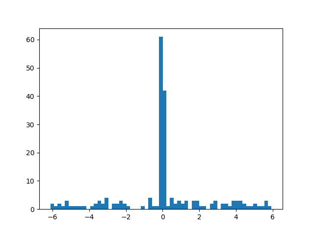
(a) $\phi_{has\_part}+\phi_{part\_of}$

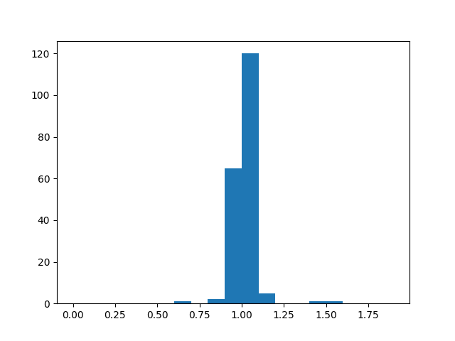
(b) $\lVert r_{has\_part}\rVert*\lVert r_{has\_part}\rVert$

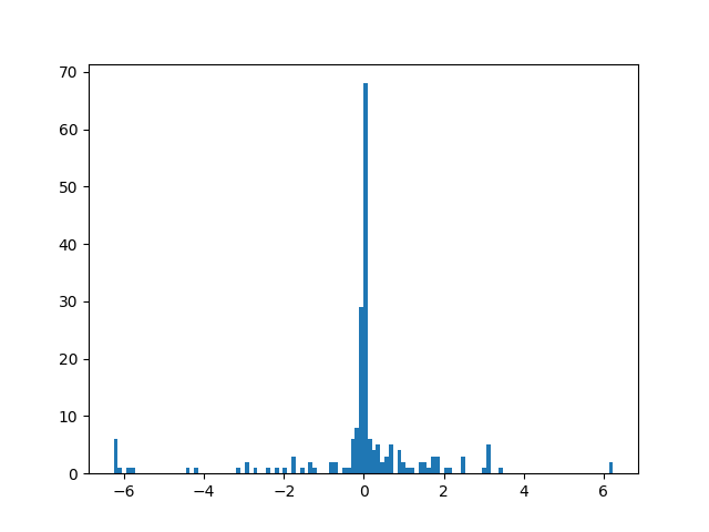
(c) $\phi(r_{1}\otimes r_{2})-\phi(r_{1})$

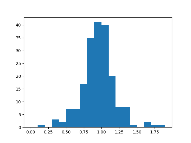
(d) $\lVert r_{part\_of}\rVert$

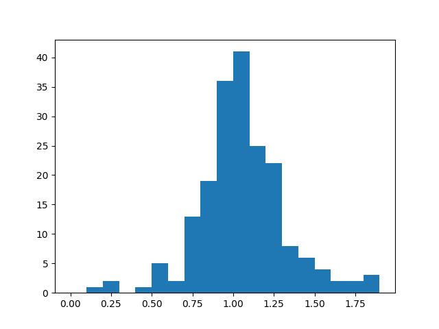
(e) $\lVert r_{has\_part}\rVert$

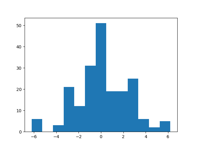
(f) $\phi(r_{1}\otimes r_{2})-\phi(r_{3})$

Figure 3. Analysis of the geometric properties of the inverse and compositional relations.

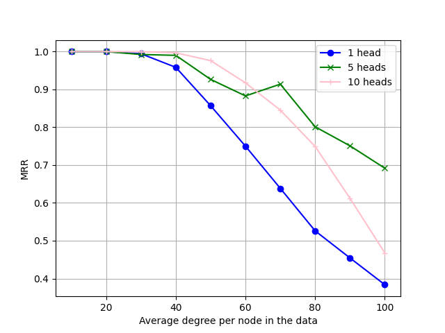
(a)

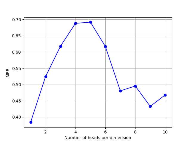
(b)

Figure 4. Effect of attribute heads on the performance.

Relation wise performance: Previous ablation study established that the geometric interpretability remains intact for HopfE. Now, we study expressiveness in a higher dimension (in addition to Table 2 and Table 4). We perform a relation-wise performance on the WN18RR dataset to understand if HopfE can maintain expressiveness compared to rotational methods which are in the lower dimensions. We borrow experimental settings from RotatE (Sun et al., 2018). As seen in Table 6, in comparison to the RotatE baseline (considering NagE skips this analysis), the HopfE model can perform better on these relations. The observed behavior implies that when we aim for geometric interpretation using Hopf Fibration, the performance does not decrease for any relation.
Studying the effect of the number of heads: In a real-world scenario, all KG entities will not have the same number of properties, and few of them may require a large number of attributes to model the KG ontology. In this experiment, we aim to understand how does adding more entity attributes for modeling dense relations impacts performance (cf., Claim 5.1)? Hence, we study the effect of increasing the number of heads on the prediction performance using a synthetic dataset because this dataset allows us to have varying number of attribute of the entities. Specifically, we generate an Erdős–Rényi graph (Erdös and Rényi, 2011) with an average degree varying from 10 to 100 in the increments of 10 steps. We use 1, 5, and 10 heads per entity per fiber(dimension). Also, note that since these are random graphs, we evaluate the performance on the train set as the performance on the test set is expected to be low in this setting. The dimensions(=10) and other common parameters are kept the same in all the models. The models are not all trained to convergence but for a fixed number of iterations. The Figure 4(a) illustrates that increasing the degree of nodes in the data in general results in a drop in the results, which is as expected. Another observation is that the setting with five heads can perform better than the one with ten heads at higher degrees. The observation possibly indicates that the latter model may require more training to fit better. A similar observation could be gleaned from Figure 4(b) where we study the effect of increasing the number of heads from 1 to 10 for a graph with an average degree per node as 100. We see that the metric improves from 1 to 5 heads and then begins to drop. We conclude that number of heads along with the training steps is a hyperparameter to be tuned for better results.

8. Conclusion

Our central research question was to study if a KGE approach can achieve geometric interpretability along with the expressiveness of four-dimensional space. The proposed theoretical foundations and associated empirical results of HopfE show that it is possible to maintain the geometric interpretability and simultaneously increase the model’s expressiveness in four-dimensional space. Furthermore, HopfE enables encoding of the entity attributes to a fibration in a higher dimension for enriching the embeddings with the semantic information prevalent in real-world KGs. Our ablation studies systematically support several choices we made in the paper’s scope, such as the use of Hopf Fibration, the effect of a number of heads, and the individual impact of entity semantic properties. Besides providing empirical evidences complementing the theoretical foundations (Sections 4 and 5), our results open up important research questions for future research: 1) In four dimensions space, how to utilize the semantic attributes (an essential aspect of KGE (Paulheim, 2018)) more optimally to positively impacting the link prediction performance and induce semantic class hierarchies similar to (Zhang et al., 2020a). 2) How to utilize logic on the attributes (or description logic) for fine-grained reasoning and logical interpretability of a KGE model in 4D? We point readers to the open research directions as viable next steps.

References

- (1)
- Allen et al. (2021) Carl Allen, I Balazevic, and Timothy Hospedales. 2021. Interpreting knowledge graph relation representation from word embeddings. In International Conference on Learning Representations.
- Bastos et al. (2021) Anson Bastos, Abhishek Nadgeri, Kuldeep Singh, Isaiah Onando Mulang, Saeedeh Shekarpour, Johannes Hoffart, and Manohar Kaul. 2021. RECON: Relation Extraction using Knowledge Graph Context in a Graph Neural Network. In Proceedings of The Web Conference (WWW).
- Baues and Baues (1989) Hans J Baues and Hans Joachim Baues. 1989. Algebraic homotopy. Vol. 15. Cambridge university press.
- Bollacker et al. (2007) Kurt D. Bollacker, Robert P. Cook, and Patrick Tufts. 2007. Freebase: A Shared Database of Structured General Human Knowledge. In AAAI.
- Bordes et al. (2013) Antoine Bordes, Nicolas Usunier, Alberto Garcia-Duran, Jason Weston, and Oksana Yakhnenko. 2013. Translating embeddings for modeling multi-relational data. In NeurlPS. 1–9.
- Chami et al. (2020) Ines Chami, Adva Wolf, Da-Cheng Juan, Frederic Sala, Sujith Ravi, and Christopher Ré. 2020. Low-Dimensional Hyperbolic Knowledge Graph Embeddings. In Proceedings of the 58th Annual Meeting of the Association for Computational Linguistics. 6901–6914.
- Cuturi (2013) Marco Cuturi. 2013. Sinkhorn distances: Lightspeed computation of optimal transport. Advances in neural information processing systems 26 (2013), 2292–2300.
- Erdös and Rényi (2011) Paul Erdös and Alfréd Rényi. 2011. On the evolution of random graphs. In The structure and dynamics of networks. Princeton University Press, 38–82.
- Gao et al. (2020) Chang Gao, Chengjie Sun, Lili Shan, Lei Lin, and Mingjiang Wang. 2020. Rotate3D: Representing Relations as Rotations in Three-Dimensional Space for Knowledge Graph Embedding. In Proceedings of the 29th ACM International Conference on Information & Knowledge Management. 385–394.
- Garcia-Duran and Niepert (2017) Alberto Garcia-Duran and Mathias Niepert. 2017. Kblrn: End-to-end learning of knowledge base representations with latent, relational, and numerical features. arXiv preprint arXiv:1709.04676 (2017).
- Gesese et al. (2019) Genet Asefa Gesese, Russa Biswas, Mehwish Alam, and Harald Sack. 2019. A survey on knowledge graph embeddings with literals: Which model links better literal-ly? Semantic Web Preprint (2019), 1–31.
- Hamilton (1844) William Rowan Hamilton. 1844. LXXVIII. On quaternions; or on a new system of imaginaries in Algebra: To the editors of the Philosophical Magazine and Journal. The London, Edinburgh, and Dublin Philosophical Magazine and Journal of Science 25, 169 (1844), 489–495.
- He et al. (2015) Kaiming He, Xiangyu Zhang, Shaoqing Ren, and Jian Sun. 2015. Delving deep into rectifiers: Surpassing human-level performance on imagenet classification. In Proceedings of the IEEE international conference on computer vision. 1026–1034.
- Hopf (1931) H Hopf. 1931. About the mapping of the three-dimensional sphere onto the spherical surface. Math. Ann. 104 (1931), 637–665.
- Ji et al. (2016) Guoliang Ji, Kang Liu, Shizhu He, and Jun Zhao. 2016. Knowledge graph completion with adaptive sparse transfer matrix. In Proceedings of the AAAI Conference on Artificial Intelligence, Vol. 30.
- Ji et al. (2021) Shaoxiong Ji, Shirui Pan, Erik Cambria, Pekka Marttinen, and Philip S Yu. 2021. A survey on knowledge graphs: Representation, acquisition and applications. EEE Transactions on Neural Networks and Learning Systems (2021).
- Kingma and Ba (2015) Diederik P. Kingma and Jimmy Ba. 2015. Adam: A Method for Stochastic Optimization. In ICLR.
- Kristiadi et al. (2019) Agustinus Kristiadi, Mohammad Asif Khan, Denis Lukovnikov, Jens Lehmann, and Asja Fischer. 2019. Incorporating literals into knowledge graph embeddings. In International Semantic Web Conference. Springer, 347–363.
- Li (NA) Samuel J. Li. NA. Hopf Fibration Visualization. https://samuelj.li/hopf-fibration/
- Lin et al. (2016) Yankai Lin, Zhiyuan Liu, and Maosong Sun. 2016. Knowledge representation learning with entities, attributes and relations. ethnicity 1 (2016), 41–52.
- Lin et al. (2015) Yankai Lin, Zhiyuan Liu, Maosong Sun, Yang Liu, and Xuan Zhu. 2015. Learning entity and relation embeddings for knowledge graph completion. In Proceedings of the AAAI Conference on Artificial Intelligence, Vol. 29.
- Lu and Hu (2020) Haonan Lu and Hailin Hu. 2020. DensE: An Enhanced Non-Abelian Group Representation for Knowledge Graph Embedding. arXiv preprint arXiv:2008.04548 (2020).
- Lu et al. (2019) Xiaolu Lu, Soumajit Pramanik, Rishiraj Saha Roy, Abdalghani Abujabal, Yafang Wang, and Gerhard Weikum. 2019. Answering complex questions by joining multi-document evidence with quasi knowledge graphs. In Proceedings of the 42nd International ACM SIGIR Conference on Research and Development in Information Retrieval. 105–114.
- Lyons (2003) David W Lyons. 2003. An elementary introduction to the Hopf fibration. Mathematics magazine 76, 2 (2003), 87–98.
- Marsden and Ratiu (1995) Jerrold E Marsden and Tudor S Ratiu. 1995. Introduction to mechanics and symmetry. Physics Today 48, 12 (1995), 65.
- Mikolov et al. (2013) Tomas Mikolov, Kai Chen, Greg Corrado, and Jeffrey Dean. 2013. Efficient Estimation of Word Representations in Vector Space. arXiv preprint arXiv:1301.3781 (2013).
- Monge (1781) Gaspard Monge. 1781. Memoir on the theory of cuttings and embankments. Histoire de l’Acad ’e mie Royale des Sciences de Paris (1781).
- Mosseri and Dandoloff (2001) Rémy Mosseri and Rossen Dandoloff. 2001. Geometry of entangled states, Bloch spheres and Hopf fibrations. Journal of Physics A: Mathematical and General 34, 47 (2001), 10243.
- PALMONARI and MINERVINI (2020) Matteo PALMONARI and Pasquale MINERVINI. 2020. Knowledge graph embeddings and explainable AI. Knowledge Graphs for Explainable Artificial Intelligence: Foundations, Applications and Challenges 47 (2020), 49.
- Paulheim (2018) Heiko Paulheim. 2018. Make embeddings semantic again!. In International Semantic Web Conference (P&D/Industry/BlueSky).
- Pennington et al. (2014) Jeffrey Pennington, Richard Socher, and Christopher D. Manning. 2014. Glove: Global Vectors for Word Representation. In Proceedings of the 2014 Conference on Empirical Methods in Natural Language Processing, EMNLP 2014, A meeting of SIGDAT, a Special Interest Group of the ACL. ACL, 1532–1543.
- Pugh and Pugh (2002) Charles Chapman Pugh and CC Pugh. 2002. Real mathematical analysis. Vol. 2011. Springer.
- Ruffinelli et al. (2019) Daniel Ruffinelli, Samuel Broscheit, and Rainer Gemulla. 2019. You can teach an old dog new tricks! on training knowledge graph embeddings. In International Conference on Learning Representations.
- Sakor et al. (2020) Ahmad Sakor, Kuldeep Singh, Anery Patel, and Maria-Esther Vidal. 2020. Falcon 2.0: An entity and relation linking tool over wikidata. In Proceedings of the 29th ACM International Conference on Information & Knowledge Management. 3141–3148.
- Sun et al. (2018) Zhiqing Sun, Zhi-Hong Deng, Jian-Yun Nie, and Jian Tang. 2018. RotatE: Knowledge Graph Embedding by Relational Rotation in Complex Space. In International Conference on Learning Representations.
- Sun et al. (2020) Zhiqing Sun, Shikhar Vashishth, Soumya Sanyal, Partha Talukdar, and Yiming Yang. 2020. A Re-evaluation of Knowledge Graph Completion Methods. In Proceedings of the 58th Annual Meeting of the Association for Computational Linguistics. 5516–5522.
- Toutanova and Chen (2015) Kristina Toutanova and Danqi Chen. 2015. Observed versus latent features for knowledge base and text inference. In Proceedings of the 3rd workshop on continuous vector space models and their compositionality. 57–66.
- Trouillon et al. (2016) Théo Trouillon, Johannes Welbl, Sebastian Riedel, Éric Gaussier, and Guillaume Bouchard. 2016. Complex embeddings for simple link prediction. In International Conference on Machine Learning. PMLR, 2071–2080.
- Vicci (2001) Leandra Vicci. 2001. Quaternions and rotations in 3-space: The algebra and its geometric interpretation. Chapel Hill, NC, USA, Tech. Rep (2001).
- Villani (2008) Cédric Villani. 2008. Optimal transport: old and new. Vol. 338. Springer Science & Business Media.
- Vrandecic (2012) Denny Vrandecic. 2012. Wikidata: a new platform for collaborative data collection. In Proceedings of the 21st World Wide Web Conference, WWW 2012 (Companion Volume). 1063–1064.
- Wang et al. (2017) Quan Wang, Zhendong Mao, Bin Wang, and Li Guo. 2017. Knowledge graph embedding: A survey of approaches and applications. IEEE Transactions on Knowledge and Data Engineering 29, 12 (2017), 2724–2743.
- Wang et al. (2018) Yanjie Wang, Rainer Gemulla, and Hui Li. 2018. On multi-relational link prediction with bilinear models. In Proceedings of the AAAI Conference on Artificial Intelligence, Vol. 32.
- Wang et al. (2016) Zhigang Wang, Juanzi Li, Zhiyuan Liu, and Jie Tang. 2016. Text-enhanced representation learning for knowledge graph. In Proceedings of International Joint Conference on Artificial Intelligent (IJCAI). 4–17.
- Wang et al. (2014) Zhen Wang, Jianwen Zhang, Jianlin Feng, and Zheng Chen. 2014. Knowledge graph embedding by translating on hyperplanes. In Proceedings of the AAAI Conference on Artificial Intelligence, Vol. 28.
- Whitney (1940) Hassler Whitney. 1940. On the theory of sphere-bundles. Proceedings of the National Academy of Sciences of the United States of America 26, 2 (1940), 148.
- Yang et al. (2015) Bishan Yang, Wen-tau Yih, Xiaodong He, Jianfeng Gao, and Li Deng. 2015. Embedding Entities and Relations for Learning and Inference in Knowledge Bases. In 3rd International Conference on Learning Representations, ICLR.
- Yang et al. (2020) Tong Yang, Long Sha, and Pengyu Hong. 2020. NagE: Non-abelian group embedding for knowledge graphs. In Proceedings of the 29th ACM International Conference on Information & Knowledge Management. 1735–1742.
- Zhang et al. (2020b) Aston Zhang, Yi Tay, SHUAI Zhang, Alvin Chan, Anh Tuan Luu, Siu Hui, and Jie Fu. 2020b. Beyond Fully-Connected Layers with Quaternions: Parameterization of Hypercomplex Multiplications with Parameters. In International Conference on Learning Representations.
- Zhang et al. (2019) Shuai Zhang, Yi Tay, Lina Yao, and Qi Liu. 2019. Quaternion Knowledge Graph Embeddings. In Advances in Neural Information Processing Systems 32: Annual Conference on Neural Information Processing Systems 2019, NeurIPS 2019. 2731–2741.
- Zhang et al. (2020a) Zhanqiu Zhang, Jianyu Cai, Yongdong Zhang, and Jie Wang. 2020a. Learning hierarchy-aware knowledge graph embeddings for link prediction. In Proceedings of the AAAI Conference on Artificial Intelligence, Vol. 34. 3065–3072.
- Zhao et al. (2020b) Feng Zhao, Tao Xu, Langjunqing Jin, and Hai Jin. 2020b. Convolutional Network Embedding of Text-enhanced Representation for Knowledge Graph Completion. IEEE Internet of Things Journal (2020).
- Zhao et al. (2020a) Yu Zhao, Ruobing Xie, Kang Liu, WANG Xiaojie, et al. 2020a. Connecting Embeddings for Knowledge Graph Entity Typing. In Proceedings of the 58th Annual Meeting of the Association for Computational Linguistics. 6419–6428.
- Zhu et al. (2018) Xuanyu Zhu, Yi Xu, Hongteng Xu, and Changjian Chen. 2018. Quaternion convolutional neural networks. In Proceedings of the European Conference on Computer Vision (ECCV). 631–647.