Minkowski–Lyapunov Functions: Alternative Characterization and Implicit Representation

Abstract

An alternative characterization of Minkowski–Lyapunov functions is derived. The derived characterization enables a computationally efficient utilization of Minkowski–Lyapunov functions in arbitrary finite dimensions. Due to intrinsic duality, the developed results apply in a direct manner to the characterization and utilization of robust positively invariant sets.

1 Background

The characterization and computation of minimal and maximal robust positively invariant sets as well as their approximations are important research themes [1, 2, 3, 4, 5, 6]. A beneficial one to one correspondence between robust positively invariant sets and Minkowski–Lyapunov functions has been established in a recent contribution [7]. The theoretical relevance of robust positively invariant sets and Minkowski–Lyapunov functions is amplified by their multifaceted practical utility. Inter alia, robust positively invariant sets can be used as the target sets for robust time optimal controllers [8], the uncertainty bounding sets for fast reference governors [9] and the tube cross–section shape sets for rigid tube model predictive controllers [10]. Likewise, Minkowski–Lyapunov functions and their sublevel sets can be used as the terminal cost functions and constraint sets for consistently improving optimal control and stabilizing model predictive control [11]. A more detailed insight into the theory, computation and applications of robust positively invariant sets and Minkowski–Lyapunov functions can be found in [1, 2, 3, 4, 5, 6, 7, 8, 9, 10, 12, 13, 11, 14] and numerous references therein.

This note addresses an apparent lack of computational methods enabling a numerically efficient utilization of robust positively invariant sets and Minkowski–Lyapunov functions in arbitrary finite dimensions. In Section 2, we derive alternative characterizations of Minkowski–Lyapunov functions and the fundamental Minkowski–Lyapunov function. In Section 3, we make use of these novel characterizations, in conjunction with implicit representations of Minkowski functions, in order to create a potent platform for a computationally efficient and dynamically compatible utilization of Minkowski–Lyapunov functions in arbitrary finite dimensions; we also discuss a method for an alternative computation of the fundamental Minkowski–Lyapunov function. In Section 4, we show that, in light of intrinsic duality [7], the derived results apply in a direct manner to robust positively invariant sets. In Section 5, we provide closing remarks including our numerical experience.

Basic Nomenclature. The spectral radius $\rho(M)$ of a matrix $M\in\mathbb{R}^{{n}\times{n}}$ is the largest absolute value of its eigenvalues. A matrix $M\in\mathbb{R}^{{n}\times{n}}$ is strictly stable if and only if $\rho(M)<1$. The Minkowski sum of nonempty sets $\mathcal{X}$ and $\mathcal{Y}$ in $\mathbb{R}^{n}$ is denoted by

$$\mathcal{X}\oplus\mathcal{Y}:=\{x+y\ :\ x\in\mathcal{X},\ y\in\mathcal{Y}\}.$$

The image $M\mathcal{X}$ and the preimage $M^{-1}\mathcal{X}$ of a nonempty set $\mathcal{X}$ under a matrix of compatible dimensions (or a scalar) $M$ are denoted, respectively, by

$$M\mathcal{X}:=\{Mx\ :\ x\in\mathcal{X}\}\text{ and }M^{-1}\mathcal{X}:=\{x\ :\ Mx\in\mathcal{X}\}.$$

A $D$–set in $\mathbb{R}^{n}$ is a closed convex subset of $\mathbb{R}^{n}$ that contains the origin. A $C$–set in $\mathbb{R}^{n}$ is a bounded $D$–set in $\mathbb{R}^{n}$. A proper $D$–set in $\mathbb{R}^{n}$ is a closed convex subset of $\mathbb{R}^{n}$ that contains the origin in its interior. A proper $C$–set in $\mathbb{R}^{n}$ is a bounded proper $D$–set in $\mathbb{R}^{n}$. The Minkowski function $\operatorname{g}(\mathcal{X},\cdot)$ of a $D$–set $\mathcal{X}$ is given, for all $y\in\mathbb{R}^{n}$, by

$$\operatorname{g}(\mathcal{X},y):=\inf_{\gamma}\{\gamma\ :\ y\in\gamma\mathcal{X},\ \gamma\geq 0\}.$$

Minkowski–Lyapunov Functions. A Minkowski–Lyapunov function [7] is the Minkowski function $\operatorname{g}(\mathcal{S},\cdot)$ of a proper $C$–set $\mathcal{S}$ in $\mathbb{R}^{n}$ that verifies the Minkowski–Lyapunov inequality

$$\forall x\in\mathbb{R}^{n},\quad\operatorname{g}(\mathcal{S},Ax)+\operatorname{g}(\mathcal{Q},x)\leq\operatorname{g}(\mathcal{S},x),$$

in which $\mathcal{Q}$ is a given proper $C$–set in $\mathbb{R}^{n}$, and which is associated with the linear dynamics

$$x^{+}=Ax,$$

where $x\in\mathbb{R}^{n}$ and $x^{+}\in\mathbb{R}^{n}$ are the current and successor states, and $A\in\mathbb{R}^{{n}\times{n}}$ is the state transition matrix. The fundamental Minkowski–Lyapunov function [7] is the Minkowski function $\operatorname{g}(\mathcal{S},\cdot)$ of a proper $C$–set $\mathcal{S}$ in $\mathbb{R}^{n}$ that verifies the Minkowski–Lyapunov equation

$$\forall x\in\mathbb{R}^{n},\quad\operatorname{g}(\mathcal{S},Ax)+\operatorname{g}(\mathcal{Q},x)=\operatorname{g}(\mathcal{S},x).$$

Explicit Representation of $D$–sets. An explicit representation of a $D$–set $\mathcal{S}$ is given by the explicit representation of its Minkowski function $\operatorname{g}(\mathcal{S},\cdot)$. In particular,

$$x\in\mathcal{S}\text{ if and only if } \operatorname{g}(\mathcal{S},x)\leq 1\text{ so that}$$

$$\mathcal{S}=\{x\in\mathbb{R}^{n}:\ \operatorname{g}(\mathcal{S},x)\leq 1\}.$$

Implicit Representation of $D$–sets. An implicit representation of a $D$–set $\mathcal{S}$ is given by an implicit representation of its Minkowski function $\operatorname{g}(\mathcal{S},\cdot)$. The implicit representations of $\mathcal{S}$ and $\operatorname{g}(\mathcal{S},\cdot)$ do not require $\mathcal{S}$ and $\operatorname{g}(\mathcal{S},\cdot)$ to be explicitly computed, as exemplified by a relatively direct variation of [15, Ch. 7, Sec. 5, Theorem 5].

Theorem 1.

Let $\{\mathcal{S}_{i}\ :\ i\in\mathcal{I}\}$ be a finite collection of $D$–sets in $\mathbb{R}^{n}$. The set

$$\mathcal{S}=\bigcap_{i\in\mathcal{I}}\mathcal{S}_{i}$$

is a $D$–set in $\mathbb{R}^{n}$. Furthermore,

$$\forall x\in\mathbb{R}^{n},\quad\operatorname{g}(\mathcal{S},x)= \max_{i\in\mathcal{I}}\operatorname{g}(\mathcal{S}_{i},x)\text{ and}$$

$$x\in\mathcal{S}\text{ if and only if } \max_{i\in\mathcal{I}}\operatorname{g}(\mathcal{S}_{i},x)\leq 1.$$

The implicit representations of the Minkowski function $\operatorname{g}(\mathcal{S},\cdot)$ and its generator set $\mathcal{S}=\bigcap_{i\in\mathcal{I}}\mathcal{S}_{i}$ are given by

$$x\mapsto \max_{i\in\mathcal{I}}\operatorname{g}(\mathcal{S}_{i},x)\text{ and}$$

$$\mathcal{S}=\{x\in\mathbb{R}^{n}:\ \max_{i\in\mathcal{I}}\operatorname{g}(\mathcal{S}_{i},x)\leq 1\}.$$

Evaluation of Minkowski Functions. Any proper $C$–polytopic set $\mathcal{P}$ has an irreducible representation (in which $\mathcal{I}_{\mathcal{P}}$ is a finite index set and each $p_{i}\in\mathbb{R}^{n}$)

$$\mathcal{P}=\{x\in\mathbb{R}^{n}\ :\ \forall i\in\mathcal{I}_{\mathcal{P}},\ p_{i}^{T}x\leq 1\}.$$

Any proper $C$–ellipsoidal set $\mathcal{E}$ centered at the origin has a representation (in which $E\in\mathbb{R}^{{n}\times{n}}$ with $E=E^{T}\succ 0$)

$$\mathcal{E}=\{x\in\mathbb{R}^{n}\ :\ \sqrt{x^{T}Ex}\leq 1\}.$$

The evaluation of $\operatorname{g}(\mathcal{P},\cdot)$ or $\operatorname{g}(\mathcal{E},\cdot)$ is highly efficient, as

$$\forall x\in\mathbb{R}^{n},\ \operatorname{g}(\mathcal{P},x)=\max_{i\in\mathcal{I}_{\mathcal{P}}}p_{i}^{T}x\text{ and }\operatorname{g}(\mathcal{E},x)=\sqrt{x^{T}Ex}.$$

The Minkowski function of the intersection of finitely many proper $C$– polytopic and/or ellipsoidal sets can be also evaluated efficiently, since, as stated in Theorem 1,

$$\forall x\in\mathbb{R}^{n},\ \operatorname{g}(\bigcap_{i\in\mathcal{I}}\mathcal{S}_{i},x)=\max_{i\in\mathcal{I}}\operatorname{g}(\mathcal{S}_{i},x).$$

Proofs. The proofs of all formal statements made in this paper are provided in the Appendix.

2 Alternative Characterization

The map $\mathcal{G}(\cdot)$ defined, for subsets $\mathcal{S}$ of $\mathbb{R}^{n}$, by

$$\mathcal{G}(\mathcal{S}):=\{x\in\mathbb{R}^{n}\ :\ \exists\gamma\in[0,1]\text{ such that }$$

$$Ax\in\gamma\mathcal{S}\text{ and }x\in(1-\gamma)\mathcal{Q}\},$$

and its post fixed points (i.e., sets such that $\mathcal{S}\subseteq\mathcal{G}(\mathcal{S})$) play a crucial role in deriving a novel, alternative, characterization of Minkowski–Lyapunov functions.

Theorem 2.

Let $A\in\mathbb{R}^{{n}\times{n}}$ and let $\mathcal{Q}$ be a proper $C$–set in $\mathbb{R}^{n}$. $(i)$ A proper $C$–set $\mathcal{S}$ in $\mathbb{R}^{n}$ is such that

$$\forall x\in\mathbb{R}^{n},\quad\operatorname{g}(\mathcal{S},Ax)+\operatorname{g}(\mathcal{Q},x)\leq\operatorname{g}(\mathcal{S},x)$$

if and only if

$$\mathcal{S}\subseteq\mathcal{G}(\mathcal{S}).$$

$(ii)$ A proper $C$–set $\mathcal{S}$ in $\mathbb{R}^{n}$ is such that $\mathcal{S}\subseteq\mathcal{G}(\mathcal{S})$ if there exists a scalar $\gamma\in[0,1]$ such that

$$A\mathcal{S}\subseteq\gamma\mathcal{S}\text{ and }\mathcal{S}\subseteq(1-\gamma)\mathcal{Q}.$$

Likewise, the map $\mathcal{G}(\cdot)$ and its maximal fixed point (in the sense that $\mathcal{S}=\mathcal{G}(\mathcal{S})$) are of paramount importance for obtaining a novel, alternative, characterization of the fundamental Minkowski–Lyapunov function.

Theorem 3.

Let $A\in\mathbb{R}^{{n}\times{n}}$ and let $\mathcal{Q}$ be a proper $C$–set in $\mathbb{R}^{n}$. $(i)$ A proper $C$–set $\mathcal{S}$ in $\mathbb{R}^{n}$ is such that

$$\forall x\in\mathbb{R}^{n},\quad\operatorname{g}(\mathcal{S},Ax)+\operatorname{g}(\mathcal{Q},x)=\operatorname{g}(\mathcal{S},x)$$

if and only if $\mathcal{S}$ is the maximal set with respect to set inclusion such that

$$\mathcal{S}=\mathcal{G}(\mathcal{S}).$$

$(ii)$ The limit, with respect to the Hausdorff distance, say $\mathcal{S}$, of the set sequence $\{\mathcal{S}_{k}\}_{k\geq 0}$, generated, for all integers $k\geq 0$, by

$$\mathcal{S}_{k+1}=\mathcal{G}(\mathcal{S}_{k})\text{ with }\mathcal{S}_{0}=\mathcal{Q},$$

is the maximal set with respect to set inclusion such that $\mathcal{S}=\mathcal{G}(\mathcal{S})$. The limit $\mathcal{S}$ is a $C$–set in $\mathbb{R}^{n}$. Furthermore, the limit $\mathcal{S}$ is a proper $C$–set in $\mathbb{R}^{n}$ if and only if $\rho(A)<1$.

3 Implicit Representation and Computation

Theorem 4 identifies a dynamically compatible parametrization of Minkowski–Lyapunov functions $\operatorname{g}(\mathcal{S},\cdot)$.

Theorem 4.

Let $A\in\mathbb{R}^{{n}\times{n}}$ be a strictly stable matrix and let $\mathcal{Q}$ be a proper $C$–set in $\mathbb{R}^{n}$. For all $\gamma\in(\rho(A),1)$, there exists a finite integer $k>0$ such that

$$(\gamma^{-1}A)^{k}\mathcal{Q}\subseteq\mathcal{Q}.$$

Furthermore, for all such scalars $\gamma\in(\rho(A),1)$ and integers $k>0$, the set

$$\mathcal{S}=(1-\gamma)\bigcap_{i=0}^{k-1}\left((\gamma^{-1}A)^{-i}\mathcal{Q}\right)$$

is a proper $C$–set in $\mathbb{R}^{n}$ such that $\mathcal{S}\subseteq\mathcal{G}(\mathcal{S})$.

Theorem 5 enables an efficient utilization of these parameterized Minkowski–Lyapunov functions $\operatorname{g}(\mathcal{S},\cdot)$.

Theorem 5.

Let $\{M_{i}\in\mathbb{R}^{{n}\times{n}}\ :\ i\in\mathcal{I}\}$ and $\{\mathcal{S}_{i}\ :\ i\in\mathcal{I}\}$ be finite collections of matrices and proper $C$–sets in $\mathbb{R}^{n}$, respectively. The set

$$\mathcal{S}=\bigcap_{i\in\mathcal{I}}M_{i}^{-1}\mathcal{S}_{i}$$

is a proper $D$–set in $\mathbb{R}^{n}$, which is a proper $C$–set in $\mathbb{R}^{n}$ when it is bounded. Furthermore,

$$\forall x\in\mathbb{R}^{n},\quad\operatorname{g}(\mathcal{S},x)= \max_{i\in\mathcal{I}}\operatorname{g}(\mathcal{S}_{i},M_{i}x)\text{ and}$$

$$x\in\mathcal{S}\text{ if and only if } \max_{i\in\mathcal{I}}\operatorname{g}(\mathcal{S}_{i},M_{i}x)\leq 1.$$

Remark 1.

Evidently, in light of Theorems 4 and 5, with $\mathcal{I}=\{0,1,\ldots,k-1\}$,

$$\forall x\in\mathbb{R}^{n},\ \operatorname{g}(\mathcal{S},x)=(1-\gamma)^{-1} \max_{i\in\mathcal{I}}\operatorname{g}(\mathcal{Q},(\gamma^{-1}A)^{i}x)\text{ and}$$

$$x\in\mathcal{S}\text{ if and only if }(1-\gamma)^{-1} \max_{i\in\mathcal{I}}\operatorname{g}(\mathcal{Q},(\gamma^{-1}A)^{i}x)\leq 1.$$

Hence, the implicit representations of Minkowski–Lyapunov functions $\operatorname{g}(\mathcal{S},\cdot)$ and their generator sets $\mathcal{S}$ characterized in Theorem 4 are given, respectively, by

$$x\mapsto(1-\gamma)^{-1} \max_{i\in\mathcal{I}}\operatorname{g}(\mathcal{Q},(\gamma^{-1}A)^{i}x)\text{ and}$$

$$\mathcal{S}=\{x\in\mathbb{R}^{n}:\ (1-\gamma)^{-1} \max_{i\in\mathcal{I}}\operatorname{g}(\mathcal{Q},(\gamma^{-1}A)^{i}x)\leq 1\}.$$

We identify one more dynamically compatible parametrization of Minkowski–Lyapunov functions $\operatorname{g}(\mathcal{S},\cdot)$. First, we recall that the polar set $\mathcal{X}^{*}$ of a set $\mathcal{X}$ in $\mathbb{R}^{n}$ with $0\in\mathcal{X}$ is

$$\mathcal{X}^{*}:=\{y\in\mathbb{R}^{n}\ :\ \forall x\in\mathcal{X},\ y^{T}x\leq 1\}.$$

Theorem 6.

Let $A\in\mathbb{R}^{{n}\times{n}}$ be a strictly stable matrix and let $\mathcal{Q}$ be a proper $C$–set in $\mathbb{R}^{n}$. For all $\gamma\in(0,1)$, there exists a finite integer $k>0$ such that

$$(A^{T})^{k}\mathcal{Q}^{*}\subseteq\gamma\mathcal{Q}^{*}.$$

Furthermore, for all such scalars $\gamma\in(0,1)$ and integers $k>0$, the set

$$\mathcal{S}=\left((1-\gamma)^{-1}\bigoplus_{i=0}^{k-1}(A^{T})^{i}\mathcal{Q}^{*}\right)^{*}$$

is a proper $C$–set in $\mathbb{R}^{n}$ such that $\mathcal{S}\subseteq\mathcal{G}(\mathcal{S})$.

We also enable an efficient use of these parameterized Minkowski–Lyapunov functions $\operatorname{g}(\mathcal{S},\cdot)$.

Theorem 7.

Let $\{M_{i}\in\mathbb{R}^{{n}\times{n}}\ :\ i\in\mathcal{I}\}$ and $\{\mathcal{S}_{i}\ :\ i\in\mathcal{I}\}$ be finite collections of matrices and proper $C$–sets in $\mathbb{R}^{n}$, respectively. The set

$$\mathcal{S}=\left(\bigoplus_{i\in\mathcal{I}}M_{i}^{T}\mathcal{S}_{i}^{*}\right)^{*}$$

is a proper $D$–set in $\mathbb{R}^{n}$, which is a proper $C$–set in $\mathbb{R}^{n}$ when it is bounded. Furthermore,

$$\forall x\in\mathbb{R}^{n},\quad\operatorname{g}(\mathcal{S},x)= \sum_{i\in\mathcal{I}}\operatorname{g}(\mathcal{S}_{i},M_{i}x)\text{ and}$$

$$x\in\mathcal{S}\text{ if and only if } \sum_{i\in\mathcal{I}}\operatorname{g}(\mathcal{S}_{i},M_{i}x)\leq 1.$$

Remark 2.

Clearly, in view of Theorems 6 and 7, with $\mathcal{I}=\{0,1,\ldots,k-1\}$,

$$\forall x\in\mathbb{R}^{n},\ \operatorname{g}(\mathcal{S},x)=(1-\gamma)^{-1} \sum_{i\in\mathcal{I}}\operatorname{g}(\mathcal{Q},A^{i}x)\text{ and}$$

$$x\in\mathcal{S}\text{ if and only if }(1-\gamma)^{-1} \sum_{i\in\mathcal{I}}\operatorname{g}(\mathcal{Q},A^{i}x)\leq 1.$$

Thus, the implicit representations of the Minkowski–Lyapunov functions $\operatorname{g}(\mathcal{S},\cdot)$ and their generator sets $\mathcal{S}$ characterized in Theorem 6 are given, respectively, by

$$x\mapsto(1-\gamma)^{-1} \sum_{i\in\mathcal{I}}\operatorname{g}(\mathcal{Q},A^{i}x)\text{ and}$$

$$\mathcal{S}=\{x\in\mathbb{R}^{n}:\ (1-\gamma)^{-1} \sum_{i\in\mathcal{I}}\operatorname{g}(\mathcal{Q},A^{i}x)\leq 1\}.$$

Remark 3.

The pointwise evaluation of the implicit representations $x\mapsto(1-\gamma)^{-1}\max_{i\in\mathcal{I}}\operatorname{g}(\mathcal{Q},(\gamma^{-1}A)^{i}x)$ and $x\mapsto(1-\gamma)^{-1}\sum_{i\in\mathcal{I}}\operatorname{g}(\mathcal{Q},A^{i}x)$ of Minkowski–Lyapunov functions $\operatorname{g}(\mathcal{S},\cdot)$ characterized in Theorems 4 and 6, respectively, is efficient in arbitrary finite dimensions for a rich variety of the proper $C$–sets $Q$. It is very simple and highly efficient when $\mathcal{Q}$ is a proper $C$–set that is either polytopic or ellipsoidal set or the intersection of polytopic and/or ellipsoidal sets. (See remarks on the evaluation of Minkowski functions in Section 1.) In particular, depending on the considered case, for a given $x$, one generates the sequence of points $\{(\gamma^{-1}A)^{i}x\}_{i=0}^{k-1}$ or $\{A^{i}x\}_{i=0}^{k-1}$ and evaluates the sequence of values $\{(1-\gamma)^{-1}\operatorname{g}(\mathcal{Q},(\gamma^{-1}A)^{i}x)\}_{i=0}^{k-1}$ or $\{(1-\gamma)^{-1}\operatorname{g}(\mathcal{Q},A^{i}x)\}_{i=0}^{k-1}$, and then computes the maximum or the sum of the latter sequence.

Remark 4.

In order to utilize the implicit representations of Minkowski–Lyapunov functions $\operatorname{g}(\mathcal{S},\cdot)$ characterized in Theorems 4 and 6, all what is needed is to detect an integer (possibly the minimal integer) $k$ for which the conditions postulated in Theorems 4 and 6 hold true. These conditions take a generic form $M^{k}\mathcal{X}\subseteq\mathcal{X}$ for a strictly stable matrix $M\in\mathbb{R}^{{n}\times{n}}$ and a proper $C$–set $\mathcal{X}$ in $\mathbb{R}^{n}$. Such a set inclusion can be also handled efficiently in arbitrary finite dimensions for a rich variety of the proper $C$–sets $\mathcal{X}$. In particular, for a proper $C$–ellipsoidal set $\mathcal{X}=\{x\ :\ \sqrt{x^{T}Xx}\leq 1\}$, such a set inclusion is equivalent to $(M^{k})^{T}XM^{k}-X\preceq 0$, which can be checked, for instance, by evaluating the eigenvalues of the matrix $(M^{k})^{T}XM^{k}-X$. Likewise, for a proper $C$–polytopic set $\mathcal{X}$ with an irreducible representation $\mathcal{X}=\{x\ :\ \forall i\in\mathcal{I}_{\mathcal{X}},\ x_{i}^{T}x\leq 1\}$, such a set inclusion holds true if and only if, for all $i\in\mathcal{I}_{\mathcal{X}}$, $\operatorname{h}(\mathcal{X},(M^{k})^{T}x_{i})\leq 1$, where $\operatorname{h}(\mathcal{X},\cdot)$ is the support function (defined in the next page) and which can be checked, for example, by solving $\operatorname{cardinality}(\mathcal{I}_{\mathcal{X}})$ linear programming problems. The above observations can be combined so as to address (via sufficiency) the case when $\mathcal{X}$ is the intersection of finitely many proper $C$– polytopic and/or ellipsoidal sets.

Theorem 3 characterizes the generator set $\mathcal{S}$ of the fundamental Minkowski–Lyapunov function $\operatorname{g}(\mathcal{S},\cdot)$ as the maximal fixed point of the map $\mathcal{G}(\cdot)$, which is the limit, with respect to the Hausdorff distance [16], of the set sequence $\{\mathcal{S}_{k}\}_{k\geq 0}$ generated by the set recursion specified in Theorem 3$(ii)$. This characterization and the corresponding set recursion can be seen as a constructive utilization of the Tarski fixed point theorem [17] and the Kleene–like iteration [18]. Note that, for any strictly stable matrix $A\in\mathbb{R}^{{n}\times{n}}$ and any proper $C$–set $\mathcal{Q}$ in $\mathbb{R}^{n}$, the sets $\mathcal{S}_{k},\ k\geq 0$ are proper $C$–sets in $\mathbb{R}^{n}$ such that $\mathcal{S}_{k+1}\subseteq\mathcal{S}_{k}$ and their limit $\mathcal{S}$ is a proper $C$–set in $\mathbb{R}^{n}$. The limit $\mathcal{S}$ is finitely determined when $\mathcal{S}_{k}\subseteq\mathcal{S}_{k+1}$ for an integer $k\geq 0$, in which case $\mathcal{S}=\mathcal{S}_{k}=\mathcal{S}_{k+1}$. This set recursion is the iterative evaluation of the map $\mathcal{G}(\cdot)$ at $\mathcal{Q}$. Its worst case computational complexity can be considerable in general. Consequently, its numerically plausible implementation should take advantage of any available structure of the matrix $A$ and proper $C$–set $\mathcal{Q}$.

4 Intrinsic Duality Implications

By [7, Theorem 1], the Minkowski function $\operatorname{g}(\mathcal{S},\cdot)$ of a proper $C$–set $\mathcal{S}$ in $\mathbb{R}^{n}$ verifies the Minkowski–Lyapunov inequality if and only if the polar set $\mathcal{Z}=\mathcal{S}^{*}$ is such that

$$A^{T}\mathcal{Z}\oplus\mathcal{W}\subseteq\mathcal{Z}\text{ with }\mathcal{W}=\mathcal{Q}^{*}.$$

This set inclusion is a necessary and sufficient condition for a set $\mathcal{Z}$ to be a robust positively invariant set [2] for the polar linear dynamics

$$z^{+}=A^{T}z+w\text{ with }w\in\mathcal{W}=\mathcal{Q}^{*},$$

for which $z\in\mathbb{R}^{n}$, $w\in\mathbb{R}^{n}$ and $z^{+}\in\mathbb{R}^{n}$ are the polar current state and disturbance and polar successor state. By [7, Theorem 3], the Minkowski function $\operatorname{g}(\mathcal{S},\cdot)$ of a proper $C$–set $\mathcal{S}$ in $\mathbb{R}^{n}$ verifies the Minkowski–Lyapunov equation if and only if the polar set $\mathcal{Z}=\mathcal{S}^{*}$ is such that

$$A^{T}\mathcal{Z}\oplus\mathcal{W}=\mathcal{Z}\text{ with }\mathcal{W}=\mathcal{Q}^{*}.$$

This fixed point set equation is, within the considered setting, a necessary and sufficient condition [6] for a set $\mathcal{Z}$ to be the minimal (nonempty and compact) robust positively invariant set [2] for the polar linear dynamics.

The preceding facts and Theorems 2$(i)$ and 3$(i)$ yield directly alternative characterizations of robust positively invariant proper $C$–sets and the minimal robust positively invariant set (over the space of nonempty compact subsets of $\mathbb{R}^{n}$) for the polar linear dynamics.

Corollary 1.

Let $A\in\mathbb{R}^{{n}\times{n}}$ and let $\mathcal{Q}$ be a proper $C$–set in $\mathbb{R}^{n}$. $(i)$ A proper $C$–set $\mathcal{Z}$ in $\mathbb{R}^{n}$ is such that

$$A^{T}\mathcal{Z}\oplus\mathcal{W}\subseteq\mathcal{Z}\text{ with }\mathcal{W}=\mathcal{Q}^{*}$$

if and only if its polar set $\mathcal{Z}^{*}$ is such that $\mathcal{Z}^{*}\subseteq\mathcal{G}(\mathcal{Z^{*}})$. $(ii)$ A proper $C$–set $\mathcal{Z}$ in $\mathbb{R}^{n}$ is such that

$$A^{T}\mathcal{Z}\oplus\mathcal{W}=\mathcal{Z}\text{ with }\mathcal{W}=\mathcal{Q}^{*}$$

if and only if its polar set $\mathcal{Z}^{*}$ is the maximal set with respect to set inclusion such that $\mathcal{Z}^{*}=\mathcal{G}(\mathcal{Z^{*}})$.

Hence, the polar sets $\mathcal{Z}=\mathcal{S}^{*}$ of the proper $C$–sets $\mathcal{S}$ characterized in Theorems 4 and 6 are robust positively invariant proper $C$–sets for the polar linear dynamics. We recall that the support function of a nonempty closed convex set $\mathcal{X}$ in $\mathbb{R}^{n}$ is given, for all $y\in\mathbb{R}^{n}$, by

$$\operatorname{h}(\mathcal{X},y):=\sup_{x}\{y^{T}x\ :\ x\in\mathcal{X}\}.$$

By the virtue of [19, Theorems 1.6.1 and 1.7.6], the support functions $\operatorname{h}(\mathcal{Z},\cdot)$ of the polar sets $\mathcal{Z}=\mathcal{S}^{*}$ of the proper $C$–sets $\mathcal{S}$ characterized in Theorems 4 and 6 satisfy $\operatorname{h}(\mathcal{Z},x)=\operatorname{g}(\mathcal{Z}^{*},x)=\operatorname{g}(\mathcal{S},x)$ for all $x\in\mathbb{R}^{n}$, and, thus, are given, respectively, by

$$\forall x\in\mathbb{R}^{n},\quad\operatorname{h}(\mathcal{Z},x)=(1-\gamma)^{-1} \max_{i\in\mathcal{I}}\operatorname{g}(\mathcal{Q},(\gamma^{-1}A)^{i}x)\text{ and}$$

$$\forall x\in\mathbb{R}^{n},\quad\operatorname{h}(\mathcal{Z},x)=(1-\gamma)^{-1} \sum_{i\in\mathcal{I}}\operatorname{g}(\mathcal{Q},A^{i}x),$$

which reveals directly their efficient implicit representations, and which when substituted in

$$\mathcal{Z}=\{x\in\mathbb{R}^{n}:\ \forall y\in\mathbb{R}^{n},\ y^{T}x\leq\operatorname{h}(\mathcal{Z},y)\}$$

yields the efficient implicit representations of the related robust positively invariant proper $C$–sets $\mathcal{Z}=\mathcal{S}^{*}$.

5 Closing Remarks and Numerical Experience

Even the computation of polyhedral positively invariant sets [20] and Lyapunov functions are relevant and active research topics. For a plethora of theoretical and computational contributions, see, for instance, [12, 13, 14] and references therein. In relation to the existing methods, and as discussed more formally in Remarks 3 and 4, the implicit representations of Minkowski–Lyapunov functions identified in Theorems 4 and 6 (and, by intrinsic duality, the corresponding robust positively invariant sets) are numerically potent in arbitrary finite dimensions. Furthermore, their structure is flexible since it is neither restricted to polytopic nor ellipsoidal proper $C$–sets.

Table 1 summarizes the outcome of a numerical test with a sample of randomly generated strictly stable matrices

$n$	$2$	$3$	$5$	$8$	$13$	$21$	$34$
$\rho(A)$	$0.977$	$0.986$	$0.982$	$0.985$	$0.993$	$0.978$	$0.981$
$k$	$16$	$19$	$44$	$57$	$100$	$50$	$84$
$t$	$0.1$	$0.3$	$0.1$	$0.2$	$0.6$	$0.7$	$3.5$
$n$	$55$	$89$	$144$	$233$	$377$	$610$	$987$
$\rho(A)$	$0.999$	$0.992$	$0.999$	$0.998$	$0.998$	$0.995$	$0.991$
$k$	$955$	$270$	$1272$	$801$	$811$	$624$	$351$
$t$	$116$	$82.9$	$1430$	$3308$	$17275$	$56512$	$122139$

Table 1. MATLAB computations for sets $\mathcal{S}$ of Theorem 4.

$A\in\mathbb{R}^{{n}\times{n}}$ for which $\rho(A)\in[0.975,0.999]$, and with $\mathcal{Q}=\mathcal{B}^{n}_{\infty}:=\{x\in\mathbb{R}^{n}\ :\ \|x\|_{\infty}\leq 1\}$ and $\gamma=(\rho(A)+1)/2$. Table 1 reports the spectral radius $\rho(A)$, the minimal integer $k$ needed to construct the implicit representations of the related Minkowski–Lyapunov functions $\operatorname{g}(\mathcal{S},\cdot)$, and the time in milliseconds (ms) needed to compute such an integer $k$ by means of a direct incremental search. The computational times vary from $0.1\ ms$ for $2$–dimensional and $5$–dimensional examples to $122139\ ms$ (i.e., about $2$ minutes and $2$ seconds) for $987$–dimensional example. Clearly, the data reported in Table 1 furnishes strong evidence of the asserted numerical potency of Minkowski–Lyapunov functions characterized in Theorem 4.

Theorem 3 delivers an alternative approach for the computation of the fundamental Minkowski–Lyapunov function and, by intrinsic duality, of the related minimal robust positively invariant set. This approach is also novel and, more importantly, it has a potential to be numerically plausible within more structured settings.

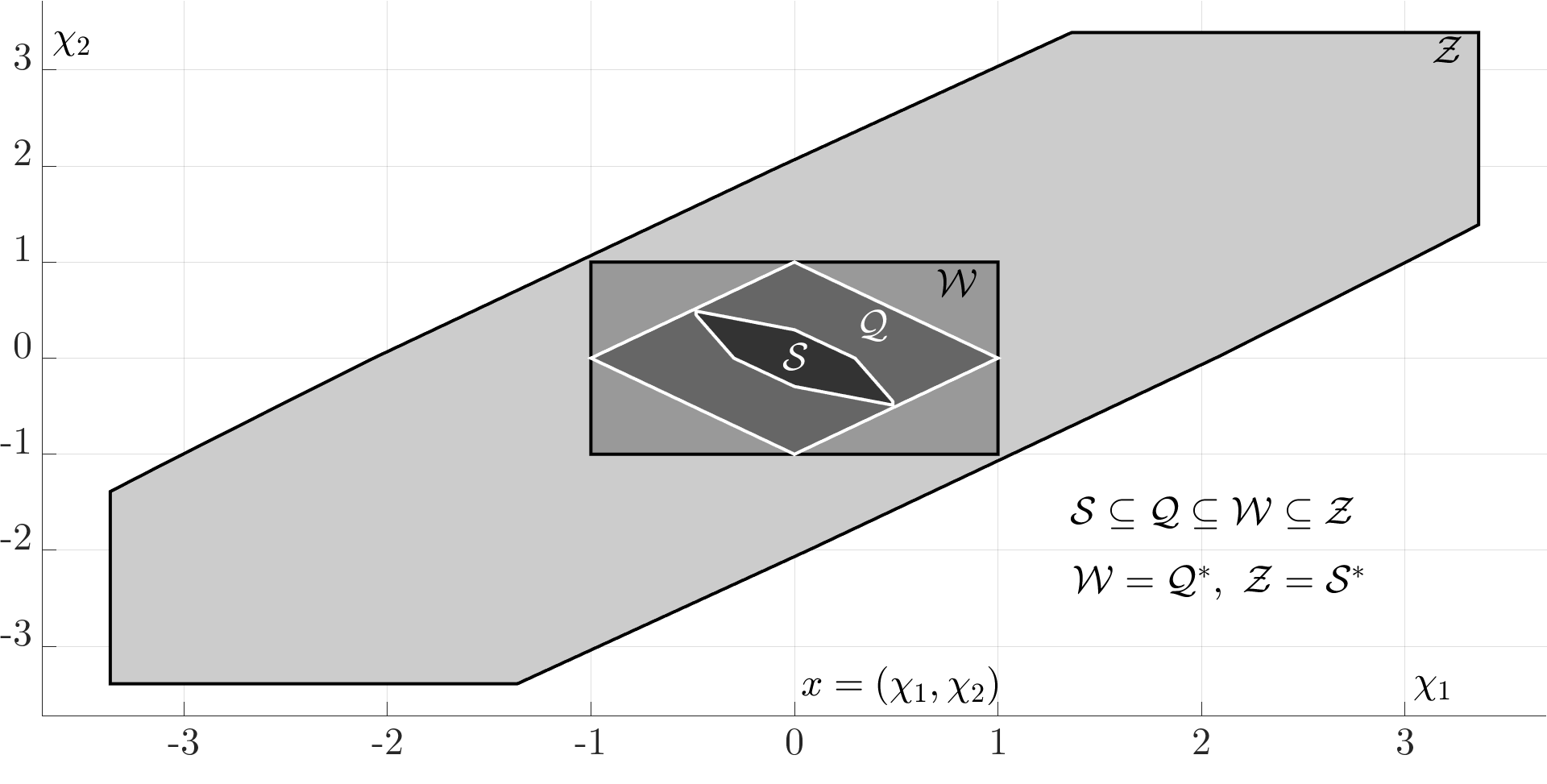
Figure 1: The Sets $\mathcal{S}$, $\mathcal{Q}$, $\mathcal{W}=\mathcal{Q}^{*}$ and $\mathcal{Z}=\mathcal{S}^{*}$.

Figure 1 illustrates the related polyhedral computations for an example, in which the entries of the matrix $A$ are $a_{(1,1)}=1$, $a_{(1,2)}=1$, $a_{(2,1)}=-0.72$, and $a_{(2,2)}=-0.7$ so that $\rho(A)=0.2$, and $\mathcal{Q}=\mathcal{B}_{1}:=\{x\ :\ \|x\|_{1}\leq 1\}$ so that $\mathcal{W}=\mathcal{Q}^{*}=\mathcal{B}_{\infty}:=\{x\ :\ \|x\|_{\infty}\leq 1\}$. The set iteration proposed in Theorem 3 generates its (numerical) limit $\mathcal{S}$ in $k=10$ steps, which is a proper $C$–polytopic set and the maximal set such that $\mathcal{S}=\mathcal{G}(\mathcal{S})$. By Corollary 1, the corresponding polar set $\mathcal{Z}=\mathcal{S}^{*}$ is the minimal proper $C$–polytopic set such that $A^{T}\mathcal{Z}\oplus\mathcal{W}=\mathcal{Z}$.

In terms of future research, a more dedicated study, with a primary focus on the related computational aspects, of a setting with a more structured matrix $A$ and the proper $C$–set $\mathcal{Q}$, would further enhance a practical utilization of Minkowski–Lyapunov functions and the fundamental Minkowski–Lyapunov function. Likewise, the study of the efficient implicit representations of the fundamental Minkowski–Lyapunov function (and, by inherent duality, the corresponding minimal robust positively invariant set) would be also of much interest.

Acknowledgement. This is an extended version of the accepted Automatica technical communiqué $20$–$1623$, which was initially submitted on November $25$, $2020$, and which is to be published by Automatica. The author is grateful to the Editor, Associate Editor and Referees for timely reviews and very constructive comments.

Appendix: Proofs

A. Proof of Theorem 1. By definition, the set $\mathcal{S}=\bigcap_{i\in\mathcal{I}}\mathcal{S}_{i}$ is at least a $D$–set in $\mathbb{R}^{n}$. By [15, Ch. 7, Sec. 5, Theorem 5], for all $x\in\mathbb{R}^{n}$, $\operatorname{g}(\mathcal{S},x)=\max_{i\in\mathcal{I}}\operatorname{g}(\mathcal{S}_{i},x)$. Hence, the claim.

B. Proof of Theorem 2. $(i)$ Since $\mathcal{S}$ and $\mathcal{Q}$ are proper $C$–sets and the Minkowski function $\operatorname{g}(\mathcal{X},\cdot)$ of a proper $C$–set $\mathcal{X}$ is positively homogeneous of the first degree, it suffices to establish the claim for an arbitrary $x$ such that $\operatorname{g}(\mathcal{S},x)=1$, so in this proof we consider such an $x$.

First, let $\mathcal{S}$ be such that $\operatorname{g}(\mathcal{S},Ax)+\operatorname{g}(\mathcal{Q},x)\leq\operatorname{g}(\mathcal{S},x)$. Let $\gamma:=\operatorname{g}(\mathcal{S},Ax)$ so that $\gamma\in[0,1]$ and $Ax\in\gamma\mathcal{S}$. Also, $\operatorname{g}(\mathcal{Q},x)\leq\operatorname{g}(\mathcal{S},x)-\operatorname{g}(\mathcal{S},Ax)=1-\gamma$ so that $x\in(1-\gamma)\mathcal{Q}$. Since $\gamma\in[0,1]$, $Ax\in\gamma\mathcal{S}$ and $x\in(1-\gamma)\mathcal{Q}$, it follows that $x\in\mathcal{G}(\mathcal{S})$. Hence, $\mathcal{S}\subseteq\mathcal{G}(\mathcal{S})$.

Second, let $\mathcal{S}$ be such that $\mathcal{S}\subseteq\mathcal{G}(\mathcal{S})$. Then there exists a $\gamma\in[0,1]$ such that $Ax\in\gamma\mathcal{S}$ and $x\in(1-\gamma)\mathcal{Q}$. In turn, $\operatorname{g}(\mathcal{S},Ax)\leq\gamma$ and $\operatorname{g}(\mathcal{Q},x)\leq 1-\gamma$. Consequently, $\operatorname{g}(\mathcal{S},Ax)+\operatorname{g}(\mathcal{Q},x)\leq\gamma+(1-\gamma)=1=\operatorname{g}(\mathcal{S},x)$. Hence, $\mathcal{S}$ is such that $\operatorname{g}(\mathcal{S},Ax)+\operatorname{g}(\mathcal{Q},x)\leq\operatorname{g}(\mathcal{S},x)$.

$(ii)$ Since $\mathcal{S}$ and $\mathcal{Q}$ are proper $C$–sets, the claimed fact follows from $(i)$.

C. Proof of Theorem 3. $(i)$ This fact follows from Theorem 2$(i)$, [7, Theorems 3] and the postulated maximality of the proper $C$–set $\mathcal{S}$.

$(ii)$ The collection of all convex subsets of $\mathbb{R}^{n}$ is a complete lattice under the natural partial ordering corresponding to the set inclusion [21], and, by its definition, $\mathcal{G}(\cdot)$ maps convex subsets of $\mathbb{R}^{n}$ into convex subsets of $\mathbb{R}^{n}$ and it is monotone (i.e. $\mathcal{X}\subseteq\mathcal{Y}$ implies that $\mathcal{G}(\mathcal{X})\subseteq\mathcal{G}(\mathcal{Y})$). Thus, all postulates of the Tarski fixed point theorem [17] are satisfied, and the Tarski fixed point theorem guarantees the existence of the maximal fixed point $\mathcal{S}$ of the map $\mathcal{G}(\cdot)$ over the collection of convex subsets of $\mathbb{R}^{n}$. Since, for any subset $\mathcal{X}$ of $\mathbb{R}^{n}$, $\mathcal{G}(\mathcal{X})\subseteq\mathcal{Q}$ and $\mathcal{G}(\cdot)$ maps (proper) $C$–sets in $\mathbb{R}^{n}$ into (proper) $C$–sets in $\mathbb{R}^{n}$, the maximal fixed point $\mathcal{S}$ of $\mathcal{G}(\cdot)$ is guaranteed to be a $C$–set in $\mathbb{R}^{n}$, which is a proper $C$–set in $\mathbb{R}^{n}$ if and only if $\rho(A)<1$. Namely, when the maximal fixed point $\mathcal{S}$ of $\mathcal{G}(\cdot)$ is a proper $C$–set in $\mathbb{R}^{n}$, Minkowski–Lyapunov function $\operatorname{g}(\mathcal{S},\cdot)$ verifies the strict stability of the matrix $A$. Likewise, when the matrix $A$ is strictly stable there exists a Minkowski–Lyapunov function $\operatorname{g}(\mathcal{R},\cdot)$ generated by a proper $C$–set $\mathcal{R}$ in $\mathbb{R}^{n}$ so that $\mathcal{R}\subseteq\mathcal{G}(\mathcal{R})\subseteq\mathcal{S}=\mathcal{G}(\mathcal{S})$ and the maximal fixed point $\mathcal{S}$ of $\mathcal{G}(\cdot)$ is a proper $C$–set in $\mathbb{R}^{n}$. In either case, $\mathcal{S}\subseteq\mathcal{Q}$ and the maximal fixed point $\mathcal{S}$ of $\mathcal{G}(\cdot)$ is the limit, with respect to the Hausdorff distance [16], of the set sequence $\{\mathcal{S}_{k}\}_{k\geq 0}$ generated by the considered set recursion.

D. Proof of Theorem 4. Since $\rho(A)\in[0,1)$ and $\gamma\in(\rho(A),1)$, $\rho(\gamma^{-1}A)\in[0,1)$. Hence, since $\rho(\gamma^{-1}A)\in[0,1)$ and $\mathcal{Q}$ is a proper $C$–set in $\mathbb{R}^{n}$, there exists a finite integer $k>0$ such that $(\gamma^{-1}A)^{k}\mathcal{Q}\subseteq\mathcal{Q}$. For any such $k$ and $\gamma$, by definition, $\mathcal{S}\subseteq(1-\gamma)\mathcal{Q}$ is a proper $C$–set in $\mathbb{R}^{n}$. Since $(\gamma^{-1}A)^{k}\mathcal{Q}\subseteq\mathcal{Q}$, $\mathcal{Q}\subseteq(\gamma^{-1}A)^{-k}\mathcal{Q}$ and, thus,

$$\mathcal{S}=(1-\gamma)\bigcap_{i=0}^{k-1}(\gamma^{-1}A)^{-i}\mathcal{Q}\subseteq(1-\gamma)\bigcap_{i=1}^{k}(\gamma^{-1}A)^{-i}\mathcal{Q},$$

and the proof is concluded by noting that $A\mathcal{S}\subseteq\gamma\mathcal{S}$, as

$$A\mathcal{S} \subseteq\gamma(\gamma^{-1}A)(1-\gamma)\bigcap_{i=1}^{k}(\gamma^{-1}A)^{-i}\mathcal{Q}$$

$$\subseteq\gamma(1-\gamma)\bigcap_{i=0}^{k-1}(\gamma^{-1}A)^{-i}\mathcal{Q}=\gamma\mathcal{S}.$$

E. Proof of Theorem 5. By definition, the set $\mathcal{S}=\bigcap_{i\in\mathcal{I}}M_{i}^{-1}\mathcal{S}_{i}$ is at least a proper $D$–set in $\mathbb{R}^{n}$ and a proper $C$–set in $\mathbb{R}^{n}$ when it is bounded. By [15, Ch. 7, Sec. 5, Theorem 5], for all $x\in\mathbb{R}^{n}$, $\operatorname{g}(\mathcal{S},x)=\max_{i\in\mathcal{I}}\operatorname{g}(M_{i}^{-1}\mathcal{S}_{i},x)$. By [21, Corollary 16.3.2], for all $x\in\mathbb{R}^{n}$ and all $i\in\mathcal{I}$, $\operatorname{g}(M_{i}^{-1}\mathcal{S}_{i},x)=\operatorname{g}(\mathcal{S}_{i},M_{i}x)$. Hence,

$$\forall x\in\mathbb{R}^{n},\quad\operatorname{g}(\mathcal{S},x)= \max_{i\in\mathcal{I}}\operatorname{g}(\mathcal{S}_{i},M_{i}x)\text{ and}$$

$$x\in\mathcal{S}\text{ if and only if } \max_{i\in\mathcal{I}}\operatorname{g}(\mathcal{S}_{i},M_{i}x)\leq 1.$$

F. Proof of Theorem 6. The claimed result follows directly from [3, Theorem 1] and  [7, Theorem 1].

G. Proof of Theorem 7. By definition, the set $\mathcal{S}=\left(\bigoplus_{i\in\mathcal{I}}M_{i}^{T}\mathcal{S}_{i}^{*}\right)^{*}$ is at least a proper $D$–set in $\mathbb{R}^{n}$ and a proper $C$–set in $\mathbb{R}^{n}$ when it is bounded. By [21, Theorem 14.5] and the algebra [21, 19] of support functions, for all $x\in\mathbb{R}^{n}$,

$$\operatorname{g}(\mathcal{S},x) =\operatorname{h}(\mathcal{S}^{*},x)=\operatorname{h}(\bigoplus_{i\in\mathcal{I}}M_{i}^{T}\mathcal{S}_{i}^{*},x)=\sum_{i\in\mathcal{I}}\operatorname{h}(M_{i}^{T}\mathcal{S}_{i}^{*},x)$$

$$=\sum_{i\in\mathcal{I}}\operatorname{h}(\mathcal{S}_{i}^{*},M_{i}x)=\sum_{i\in\mathcal{I}}\operatorname{g}(\mathcal{S}_{i},M_{i}x).$$

Hence,

$$\forall x\in\mathbb{R}^{n},\quad\operatorname{g}(\mathcal{S},x)= \sum_{i\in\mathcal{I}}\operatorname{g}(\mathcal{S}_{i},M_{i}x)\text{ and}$$

$$x\in\mathcal{S}\text{ if and only if } \sum_{i\in\mathcal{I}}\operatorname{g}(\mathcal{S}_{i},M_{i}x)\leq 1.$$

H. Proof of Corollary 1. The stated facts follow from Theorems 2$(i)$ and 3$(i)$ and [7, Theorem 1 and 3].

References

- [1] V. M. Kuntsevich and B. N. Pshenichnyi. Minimal Invariant Sets of Dynamic Systems with Bounded Disturbances. Cybernetics and Systems Analysis, 32:58–64, 1996.
- [2] I. V. Kolmanovsky and E. G. Gilbert. Theory and Computation of Disturbance Invariant Sets for Discrete–Time Linear Systems. Mathematical Problems in Egineering, 4:317–367, 1998.
- [3] S. V. Raković, E. C. Kerrigan, K. I. Kouramas, and D. Q. Mayne. Invariant Approximations of the Minimal Robustly Positively Invariant Sets. IEEE Transactions on Automatic Control, 50(3):406–410, 2005.
- [4] A. Limpiyamitr and Y. Ohta. The Duality Relation between Maximal Output Admissible Set and Reachable Set. In Proceedings of the 44th IEEE Conference on Decision and Control, December 2005.
- [5] S. V. Raković. Minkowski Algebra and Banach Contraction Principle in Set Invariance for Linear Discrete Time Systems. In Proceedings of 46th IEEE Conference on Decision and Control, New Orleans, LA, USA, December 2007.
- [6] Z. Artstein and S. V. Raković. Feedback and Invariance under Uncertainty via Set Iterates. Automatica, 44(2):520–525, 2008.
- [7] S. V. Raković. Polarity of Stability and Robust Positive Invariance. Automatica, 118:109010, 2020.
- [8] D. Q. Mayne and W. R. Schroeder. Robust Time–Optimal Control of Constrained Linear Systems. Automatica, 33:2103–2118, 1997.
- [9] E. G. Gilbert and I. V. Kolmanovsky. Fast Reference Governors for Systems with State and Control Constraints and Disturbance Inputs. International Journal of Robust and Nonlinear Control, 9(15):1117–1141, 1999.
- [10] D. Q. Mayne, M. M. Seron, and S. V. Raković. Robust Model Predictive Control of Constrained Linear Systems with Bounded Disturbances. Automatica, 41(2):219–224, 2005.
- [11] J. B. Rawlings and D. Q. Mayne. Model Predictive Control: Theory and Design. Nob Hill Publishing, Madison, 2009.
- [12] F. Blanchini. Set Invariance in Control. Automatica, 35:1747–1767, 1999.
- [13] F. Blanchini and S. Miani. Set–Theoretic Methods in Control. Birkhauser, 2008.
- [14] P. Giesl and S. Hafstein. Review on Computational Methods for Lyapunov Functions. Discrete and Continuous Dynamical Systems, Series B, 20, 2015.
- [15] C. Berge. Topological Spaces. Oliver and Boyd, 1963.
- [16] E. Klein and A. C. Thompson. Theory of Correspondences. Wiley–Interscience, 1984.
- [17] A. Tarski. A Lattice-Theoretical Fixpoint Theorem and Its Applications. Pacific Journal of Mathematics, 5:285–309, 1955.
- [18] S. C. Kleene. Introduction to Metamathematics. North–Holland Publishing, 1952.
- [19] R. Schneider. Convex Bodies: The Brunn–Minkowski Theory. Cambridge University Press, 1993.
- [20] G. Bitsoris. Positive Invariant Polyhedral Sets of Discrete–Time Linear Systems. Cybernetics and Systems Analysis, 47:1713–1726, 1988.
- [21] R. T. Rockafellar. Convex Analysis. Princeton University Press, 1970.