Formation of the First Two Black Hole–Neutron Star Mergers (GW200115 and GW200105) from Isolated Binary Evolution

Abstract

In this work we study the formation of the first two black hole–neutron star (BHNS) mergers detected in gravitational waves ($\rm{GW200115}$ and $\rm{GW200105}$) from massive stars in wide isolated binary systems – the isolated binary evolution channel. We use $560$ BHNS binary population synthesis model realizations and show that the system properties (chirp mass, component masses, and mass ratios) of both $\rm{GW200115}$ and $\rm{GW200105}$ match predictions from the isolated binary evolution channel. We also show that most model realizations can account for the local BHNS merger rate densities inferred by LIGO–Virgo. However, to simultaneously also match the inferred local merger rate densities for BHBH and NSNS systems we find we need models with moderate kick velocities ($\sigma\lesssim 10^{2}$$\,\rm{km}\,\rm{s}^{-1}$) or high common-envelope efficiencies ($\alpha_{\rm{CE}}\gtrsim 2$) within our model explorations. We conclude that the first two observed BHNS mergers can be explained from the isolated binary evolution channel for reasonable model realizations.

1 Introduction

In 2021 June, Abbott et al. (2021c) announced the first observations of gravitational waves from two BHNS merger events–$\rm{GW200115}$ and $\rm{GW200105}$–during the third LIGO–Virgo–Kagra (LVK) observing run (O3). $\rm{GW200115}$ was detected by all three detectors from LIGO and Virgo and has chirp mass ${m}_{\rm{chirp}}=2.42_{-0.07}^{+0.05}$$\,\rm{M}_{\odot}$, total mass $m_{\rm{tot}}=7.1_{-1.4}^{+1.5}$$\,\rm{M}_{\odot}$, component masses $m_{\rm{BH}}=5.{7}_{-2.1}^{+1.8}$ $\,\rm{M}_{\odot}$ and $m_{\rm{NS}}=1.{5}_{-0.3}^{+0.7}$$\,\rm{M}_{\odot}$ and mass ratio $q_{\rm{f}}\equiv(m_{\rm{NS}}/m_{\rm{BH}})=0.26_{-0.10}^{+0.35}$. $\rm{GW200105}$ was effectively only observed by LIGO–Livingston as LIGO–Hanford was offline and the signal-to-noise ratio in Virgo was below the threshold of 4.0. $\rm{GW200105}$ has ${m}_{\rm{chirp}}=3.41^{+0.08}_{-0.07}$, $m_{\rm{tot}}=10.9_{-1.2}^{+1.1}$$\,\rm{M}_{\odot}$, $m_{\rm{BH}}=8.{9}_{-1.5}^{+1.2}$ $\,\rm{M}_{\odot}$, $m_{\rm{NS}}=1.{9}_{-0.2}^{+0.3}$ $\,\rm{M}_{\odot}$ and $q_{\rm{f}}=0.22_{-0.04}^{+0.08}$.

From these observations Abbott et al. (2021c) infer a local BHNS merger rate density of $\mathcal{R}_{\rm{BHNS}}={45}_{-33}^{+75}$$\,\rm{Gpc}^{-3}\,\rm{yr}^{-1}$ when assuming that $\rm{GW200115}$ and $\rm{GW200105}$ are solely representative of the entire BHNS population; and $\mathcal{R}_{\rm{BHNS}}={130}_{-69}^{+112}$$\,\rm{Gpc}^{-3}\,\rm{yr}^{-1}$ when assuming a broader distribution of component masses (Abbott et al., 2021c). For the individual $\rm{GW200115}$ and $\rm{GW200105}$ events, the authors quote inferred local merger rate densities of $\mathcal{R}_{\rm{GW200115}}={36}_{-30}^{+82}$$\,\rm{Gpc}^{-3}\,\rm{yr}^{-1}$ and $\mathcal{R}_{\rm{GW200105}}={16}_{-14}^{+38}$$\,\rm{Gpc}^{-3}\,\rm{yr}^{-1}$, respectively. In Abbott et al. (2021a), LVK reported a binary neutron star (NSNS) merger rate of $\mathcal{R}_{\rm{NSNS}}=320^{+490}_{-240}$$\,\rm{Gpc}^{-3}\,\rm{yr}^{-1}$, and four different binary black hole (BHBH) $90\%$ credible rate intervals spanning $\mathcal{R}_{\rm{BHBH}}\approx 10.3-104$$\,\rm{Gpc}^{-3}\,\rm{yr}^{-1}$.

The main formation channel leading to merging BHNS systems (and BHBH and NSNS) is still under debate. A widely studied channel is the formation of BHNS mergers from massive stars that form in (wide) isolated binaries and evolve typically including a common envelope (CE) phase (e.g. Neijssel et al., 2019; Belczynski et al., 2020; Shao & Li, 2021). Other possible channels include formation from close binaries that can evolve chemically homogeneously (Mandel & de Mink, 2016; Marchant et al., 2017), metal-poor Population III stars that formed in the early universe (e.g. Belczynski et al., 2017), stellar triples or multiples (Fragione & Loeb, 2019; Hamers & Thompson, 2019; Hamers et al., 2021), or from dynamical or hierarchical interactions in globular clusters (Clausen et al., 2013; Arca Sedda, 2020; Ye et al., 2020), nuclear star clusters (Petrovich & Antonini, 2017; McKernan et al., 2020; Wang et al., 2021) and young and/or open star clusters (e.g., Ziosi et al., 2014; Rastello et al., 2020; Arca Sedda, 2021). We refer the reader to Mandel & Broekgaarden (2021) for a living review of these various formation channels.

In this Letter we address the key question: Could GW200115 and GW200105 have been formed through the isolated binary evolution scenario?

To investigate this we use the simulations from Broekgaarden et al. (2021a) to study the formation of merging BHNS systems from pairs of massive stars that evolve through the isolated binary evolution scenario. This Letter is structured as follows. In §2 we describe our method and models. In §3.1 we show that most of our models do match the inferred BHNS rate densities, but that only models with higher CE efficiencies or moderate supernova (SN) kicks are also consistent with the inferred $\mathcal{R}_{\rm{BHBH}}$ and $\mathcal{R}_{\rm{NSNS}}$. In §3.2 we compare the properties of $\rm{GW200115}$ and $\rm{GW200105}$ to the overall expected GW-detectable BHNS population. We end with a discussion in §4 and present our conclusions in §5.

2 Method

We use the publicly available binary population synthesis simulations from Broekgaarden et al. (2021a, presented in Broekgaarden et al., in preparation), to study the formation of $\rm{GW200115}$ and $\rm{GW200105}$ from the isolated binary evolution channel. The simulations used in this work add new model realizations compared to Broekgaarden et al. (2021b), and also consider merging BHBH and NSNS systems. The simulations are performed using the rapid binary population synthesis code COMPAS (Stevenson et al., 2017b; Barrett et al., 2017; Vigna-Gómez et al., 2018; Broekgaarden et al., 2019; Neijssel et al., 2019), which is used to model the evolution of the binary systems and determine the source properties and rates of the double compact object mergers. The BHNS population data set contains a total of $560$ model realizations to explore the uncertainty in the population modeling. Namely, $20$ different binary population synthesis variations (varying assumptions for common envelope, mass transfer, supernovae, and stellar winds) and $28$ model variations in the metallicity-specific star formation rate density model, SFRD$(Z,z)$ (varying assumptions for the star formation rate density, mass-metallicity relation, and galaxy stellar mass function), which is a function of birth metallicity ($Z$) and redshift ($z$). The population synthesis simulations are labeled A, B, C, … T, with each variation representing one change in the physics prescription compared to the fiducial model ‘A’ (see Table 1 in Broekgaarden et al. in preparation); the SFRD$(Z,z)$ models are labelled with 000, 111, 112, … 333 (see Table 3 Broekgaarden et al. 2021b). To obtain high–resolution simulations, Broekgaarden et al. (in prep.) simulated for each population synthesis model a million binaries for 53 $Z$ bins and used the adaptive importance sampling algorithm STROOPWAFEL (Broekgaarden et al., 2019) to further increase the number of BHNS systems in the simulations. Doing so, resulted in a total dataset consisting of over 30 million BHNS systems, making it the most extensive simulation of its kind to date.

We define BHNS systems in our simulations to match the observed $\rm{GW200115}$ and $\rm{GW200105}$ if their ${m}_{\rm{chirp}}$, $m_{\rm{tot}}$, $m_{1,\rm{f}}$, $m_{2,\rm{f}}$ ánd $q_{\rm{f}}$ lie within the inferred $90\%$ credible intervals (§1). We note that Abbott et al. (2021c) also inferred $90\%$ credible intervals for the spins of both BHNS systems, but due to the large uncertainties in the measurements and the theory of spins we leave this topic for discussion in §4 and do not explicitly take spins into account for the BHNS system selection. We calculate $\mathcal{R}_{\rm{BHNS}}$ using Equation 2 in Broekgaarden et al. (2021b), where we assume a local redshift $z\approx 0$, and discuss these intrinsic merger rates in §3.1. We obtain the detection-weighted distributions for the BHNS mergers using Equation 3 from Broekgaarden et al. (2021b) and discuss these in §3.2. To calculate the detectable GW population we assume the sensitivity of a GW–detector network equivalent to advanced LIGO in its design configuration (Aasi et al., 2015; Abbott et al., 2016, 2018), a reasonable proxy for O3. For the purpose of comparison, we use the LIGO–Virgo posterior samples for $\rm{GW200115}$ and $\rm{GW200105}$ from Abbott et al. (2021d).

3 Predicted BHNS Merger Rates and Properties

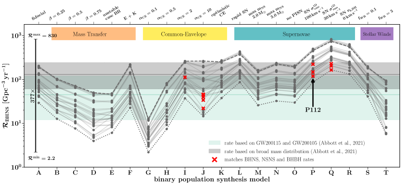
Figure 1: Predicted local BHNS merger rate density, $\mathcal{R}_{\rm{BHNS}}$, for our $560$ model variations. The shaded horizontal bars mark the corresponding GW-inferred $90\%$ credible intervals for the merger rate densities from Abbott et al. (2021c): $\mathcal{R}_{\rm{BHNS}}={45}_{-33}^{+75}$$\,\rm{Gpc}^{-3}\,\rm{yr}^{-1}$ (green) and $\mathcal{R}_{\rm{BHNS}}={130}_{-69}^{+112}$$\,\rm{Gpc}^{-3}\,\rm{yr}^{-1}$ (gray). We connect simulation predictions that use the same SFRD$(Z,z)$ model with a line for visual clarity only. Two SFRD$(Z,z)$ variations, 231 (dashed) and 312 (dotted), are highlighted. Model realizations matching one of the inferred $\mathcal{R}_{\rm{BHNS}}$ and also the $90\%$ credible intervals for the BHBH and NSNS merger rates from Abbott et al. (2021a) are marked with red crosses. In the top we added colored labels to indicate what physics assumptions are varied compared to our fiducial assumptions in the models. An arrow points to model P112 (§3.2).

3.1 Local BHNS merger rates

In Figure 1 we show the predicted local merger rate densities from our $560$ model realizations for the overall BHNS population, in comparison to the $90\%$ credible intervals from Abbott et al. (2021c). We find that the majority of the $560$ model realizations match one of the two observed BHNS merger rate densities. Model realizations that underpredict the observed rates include most SFRD$(Z,z)$ variations of model G ($\alpha_{\rm{CE}}=0.1$) corresponding to inefficient CE ejection, which increases the number of stellar mergers during the CE phase (our fiducial model uses $\alpha_{\rm{CE}}=1$), and about half of the SFRD$(Z,z)$ variations of model D, which assumes a high mass transfer efficiency ($\beta=0.75$), as opposed to our fiducial model that assumes an adaptive $\beta$ based on the stellar type and thermal timescale and typically results in $\beta\lesssim 0.1$ for systems leading to BHNS mergers. Conversely, some model realizations overpredict the observed rates, in particular about half of the SFRD$(Z,z)$ variations of models P, Q and R. These models have moderate or low SN natal kick magnitudes, increasing the number of BHNS systems that stay bound during the SNe. The SFRD$(Z,z)$ variations that overpredict the observed rates correspond to lower average metallicities, thereby increasing the formation efficiency of BHNS mergers (Broekgaarden et al., 2021b).

On the other hand, we find that only a small subset of the $560$ model realizations (shown with red crosses in Figure 1) also match the inferred $90\%$ credible intervals of the observed BHBH and NSNS merger rate densities (§1), namely, models I, J, P and Q in conjunction with a few of the SFRD$(Z,z)$ variations. Both the higher $\alpha_{\rm{CE}}$ values in models I and J ($\alpha_{\rm{CE}}\gtrsim 2$), and the low SN natal kicks in models P and Q ($\sigma\approx 30$ or $100\,\rm{km}\,\rm{s}^{-1}$, where $\sigma$ is the one-dimensional rms velocity dispersion of the Maxwellian distribution used to draw the SN natal kick magnitudes), result in relatively higher NSNS rates that can match the high observed $\mathcal{R}_{\rm{NSNS}}$ ^,. Requiring a match with the observed $\mathcal{R}_{\rm{BHBH}}$ mostly constrains the SFRD$(Z,z)$ models to those with moderate average star formation metallicities, as our models with typically lower $Z$ overestimate the inferred $\mathcal{R}_{\rm{BHBH}}$. Similar results were found by earlier work including Giacobbo & Mapelli (2018) and Santoliquido et al. (2021).

Within the matching models, models I, P and Q match the inferred $\mathcal{R}_{\rm{BHNS}}$ that is based on a broader BHNS mass distribution, whereas the matching model J variations overlap only with the observed rate based on a $\rm{GW200115}$- and $\rm{GW200105}$-like population. We note, however, that our binary population synthesis models in all cases predict a broader mass distribution compared to just $\rm{GW200115}$- and $\rm{GW200105}$-like events. We investigate this in detail in Figure 2, where we plot the cumulative BHNS chirp mass distributions of our model variations, in comparison to the chirp masses spanned by $\rm{GW200115}$ and $\rm{GW200105}$, $2.35\lesssim{m}_{\rm{chirp}}/\,\rm{M}_{\odot}\lesssim 3.49$. We find that $\approx 60\%$ of the GW-detectable BHNS systems in model J are expected to have ${m}_{\rm{chirp}}$ outside of this range, while for matching models I, P and Q this is about $60\%$, $50\%$, and $50\%$, respectively. For models I, P and Q this result is expected since they match the $\mathcal{R}_{\rm{BHNS}}$ range that is based on a broader mass distribution, but for model J the low percentage of $60\%$ conflicts the match with $\mathcal{R}_{\rm{BHNS}}$ based on a BHNS population defined by $\rm{GW200115}$- and $\rm{GW200105}$-like events. From Figure 2 it can be seen that besides models I, J, P and Q all other model realizations generally predict BHNS populations with broader chirp mass distributions compared to the range spanned by $\rm{GW200115}$ and $\rm{GW200105}$ alone. The models using the rapid supernova prescription (model L) predict the highest fraction ($\approx 75\%$) of BHNS systems with $2.35\lesssim{m}_{\rm{chirp}}/\,\rm{M}_{\odot}\lesssim 3.49$, whereas the model assuming that case BB mass transfer is always unstable (model E) results in the lowest percentages ($\approx 8\%$).

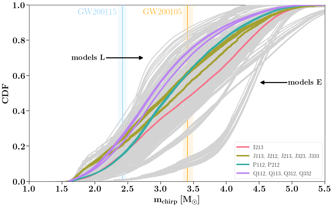
Figure 2: Cumulative distributions of the chirp mass for the models matching $\mathcal{R}_{\rm{BHNS}}$, $\mathcal{R}_{\rm{BHBH}}$ and $\mathcal{R}_{\rm{NSNS}}$ (colored lines) and all of the other $560$ model realizations (light gray lines). We also show the $90\%$ credible intervals for $\rm{GW200115}$ and $\rm{GW200105}$ (vertical bars; Abbott et al. 2021c). The legend indicates the label names of the matching models, while the arrows point to models E and L, which predict the lowest and highest fraction of BHNS mergers within the chirp mass range spanning $\rm{GW200115}$ and $\rm{GW200105}$, respectively.

3.2 Properties of the BHNS systems

In the following discussion we focus on the specific model ‘P112’, as an example of a model realization that matches all of the various observed merger rate densities. We take this approach for simplicity, but note that we are not claiming that only this model realization represents the correct isolated binary evolution pathway to the observed GW mergers. Below we examine the properties of the systems at the time of merger (chirp mass, component masses and mass ratio), as well as at the time of formation on the zero-age main sequence (ZAMS) (component masses, mass ratio and semimajor axis).

3.2.1 BHNS properties at merger

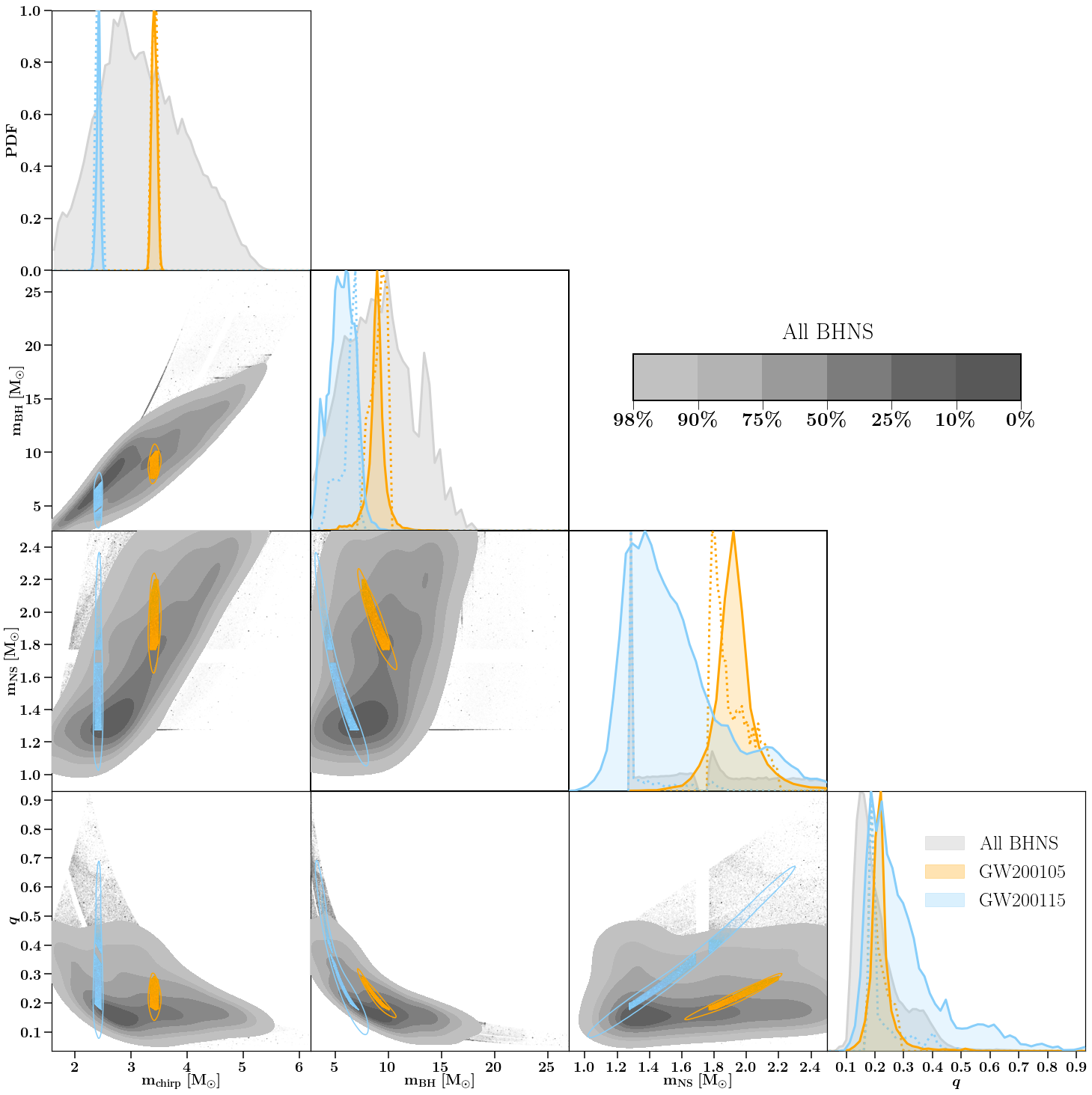
Figure 3: Corner plot showing the 1D and 2D distributions of the properties of the detectable BHNS mergers from our binary population synthesis model P112. We show the chirp mass, BH mass, NS mass, and the mass ratio at the time of merger. In gray we show the overall BHNS population, whereas in blue (orange) we show BHNS systems that have properties matching $\rm{GW200115}$ ($\rm{GW200105}$). Our $\rm{GW200115}$ ($\rm{GW200105}$) predictions are shown with blue (orange) scatter points and dotted histograms, whereas the posterior samples from Abbott et al. (2021c) are shown with $90\%$ contour levels in the 2D plots and with filled histograms in the 1D panels. The gray contours show the percentage of the detectable BHNS systems enclosed. All distributions are weighted using the GW-detection probability. The 1D distributions are normalized such that the peak is equal to one.

In Figure 3 we show the 1D and 2D distributions of the predicted properties for the GW-detectable BHNS population for all BHNS systems (gray contours and 1D distributions) and for $\rm{GW200115}$- and $\rm{GW200105}$-like BHNS systems (blue and orange scatter points and dotted histograms, respectively). The LIGO-Virgo inferred posterior samples for $\rm{GW200115}$ and $\rm{GW200105}$ are shown with orange and blue $90\%$ credible contours in the 2D histograms and with filled histograms in the 1D plots, respectively. We show ${m}_{\rm{chirp}}$, $m_{\rm{BH}}$, $m_{\rm{NS}}$ and $q_{\rm{f}}$. In the top panels we normalize each 1D distribution to peak at a value of 1.

Overall, we find that model P112 predicts the majority ($90\%$ percentiles) of the GW-detectable BHNS mergers to have $2\lesssim{m}_{\rm{chirp}}/\,\rm{M}_{\odot}\lesssim 4.6$, $4.1\lesssim m_{\rm{BH}}/\,\rm{M}_{\odot}\lesssim 14.7$, $1.3\lesssim m_{\rm{NS}}/\,\rm{M}_{\odot}\lesssim 2.4$, and $0.1\lesssim q_{\rm{f}}\lesssim 0.4$. We emphasize that the neutron star mass and lower black hole mass boundaries of $1$$\,\rm{M}_{\odot}$ and $2.5$$\,\rm{M}_{\odot}$, respectively, are set by our binary population synthesis assumptions for the lower and upper NS mass from the delayed Fryer et al. (2012) remnant mass prescription.

In detail, we find several interesting features in the model distributions compared to the observed BHNS mergers. First, we note that the inferred properties of $\rm{GW200115}$ and $\rm{GW200105}$ lie well within the predicted population of the GW-detectable BHNS population. In particular, the $\rm{GW200115}$ and $\rm{GW200105}$ credible intervals typically overlap with the highest probability region for the corresponding distribution of the predicted BHNS population. We stress that this result does not follow trivially from the match of model P112 with the inferred $\mathcal{R}_{\rm{BHNS}}$ (§3.1) as the properties of the intrinsic and detectable BHNS populations could be significantly different due to the strong bias in the sensitivity of GW detectors for more massive systems, meaning that the underlying intrinsic mass distributions can be significantly different from the observed mass distributions. Only for $m_{\rm{NS}}$ the posterior samples of $\rm{GW200115}$ reach well below the predicted distribution of our models, but this is due to the remnant mass prescription, which has an artificial lower $m_{\rm{NS}}$ limit of about $1.3$$\,\rm{M}_{\odot}$. The overlap between our predictions and the inferred posterior distributions can also be seen from the matches between the LVK distributions and our model-weighted distributions for $\rm{GW200115}$ and $\rm{GW200105}$.

Second, we find that model P112 suggests the existence of a small, positive, $m_{\rm{BH}}$–$m_{\rm{NS}}$ correlation in the GW-detectable BHNS population (a similar correlation is also visible in the ${m}_{\rm{chirp}}$–$m_{\rm{NS}}$ distribution, but we note that the chirp mass is dependent on $m_{\rm{NS}}$). This means that we expect, on average, that BHNS with more massive BHs have more massive NSs. Interestingly, this correlations also holds for $\rm{GW200115}$ and $\rm{GW200105}$. This correlation is visible in most of our other model variations, and was also noted by earlier work, including Kruckow et al. (2018) and Broekgaarden et al. (2021b). The correlation is due to the preference in the isolated binary evolution channel for more equal mass binaries. The BHNS with more massive BH typically form from binaries with a more massive primary (the initially more massive star), and such systems also have on average more massive secondaries at ZAMS (see Sana et al. 2012). In addition, the more massive secondaries at ZAMS typically lead to binaries with more equal mass ratios at the moment of the first mass transfer, making it likely more stable and successfully leading to a BHNS (Broekgaarden et al., 2021b). This results on average in a more massive NS in binaries with a more massive BH.

Finally, we note that several of the panels in Figure 3 show sharp gaps or peaks in the distributions, particularly visible in the scatter points and 1D histograms. These gaps are artificial discontinuities present in some of the prescriptions in our COMPAS model (see Broekgaarden et al., 2021b, and references therein).

3.2.2 BHNS properties at ZAMS

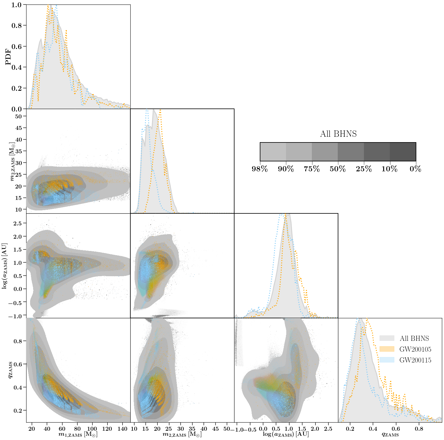
Figure 4: Same as Figure 3 but showing the binary system properties at ZAMS for the detectable BHNS population of model P112. We show the primary mass, secondary mass, semimajor axis and mass ratio. We do not show inferred credible intervals from LIGO-Virgo in this figure as the ZAMS properties are not measurable through GWs.

In Figure 4 we show the ZAMS properties of the binary systems that successfully form detectable BHNS mergers: primary mass ($m_{1,\rm{ZAMS}}$), secondary mass ($m_{2,\rm{ZAMS}}$), semimajor axis ($a_{\rm{ZAMS}}$), and mass ratio ($q_{\rm{ZAMS}}\equiv m_{2,\rm{ZAMS}}/m_{1,\rm{ZAMS}}$). In blue (orange) we show the ZAMS properties of binaries in our simulation that eventually form BHNS matching the inferred credible intervals of $\rm{GW200115}$ ($\rm{GW200105}$). The distributions are weighted for the sensitivity of a GW-detector network. Several features can be seen that we describe below.

First, we find that $\rm{GW200115}$- and $\rm{GW200105}$-like GW mergers form from binaries that have 1D distributions ($90$th percentiles) in the ranges $26\lesssim m_{1,\rm{ZAMS}}/\,\rm{M}_{\odot}\lesssim 112$, $13\lesssim m_{2,\rm{ZAMS}}/\,\rm{M}_{\odot}\lesssim 25$, $10^{0.04}\lesssim a_{\rm{ZAMS}}/\,\mathrm{AU}\lesssim 10^{1.5}$, and $0.15\lesssim q_{\rm{ZAMS}}\lesssim 0.75$. From the histograms it can be seen that the initial conditions of the binaries that form $\rm{GW200115}$- and $\rm{GW200105}$-like mergers are representative of the overall BHNS forming population.

Second, when comparing $\rm{GW200115}$ and $\rm{GW200105}$, we find that our model predicts that both systems formed from binaries with similar primary star masses. However, for the other ZAMS properties the model predicts that $\rm{GW200105}$-like BHNS mergers form from binaries with slightly larger $m_{2,\rm{ZAMS}}$, $a_{\rm{ZAMS}}$ and $q_{\rm{ZAMS}}$, compared to $\rm{GW200115}$-like BHNS mergers. The larger secondary masses for $\rm{GW200105}$ are required to form the more massive NS in this system. The larger secondary mass also causes the slight preference for larger $a_{\rm{ZAMS}}$ at ZAMS as the increased secondary mass impacts the timing of mass transfer in several ways, including the time at which the primary will fill its Roche lobe, and the common-envelope phase later on (more/less shrinking due to a different envelope mass). As a result we find that $\rm{GW200105}$-like mergers form from slightly larger $a_{\rm{ZAMS}}$ compared to $\rm{GW200115}$-like mergers.

Third, it can be seen that several of the distributions in Figure 4 show small gaps in ZAMS space that form BHNSs with combinations of BH and NS masses that do not match $\rm{GW200115}$ or $\rm{GW200105}$. These are mostly a consequence from small regions in $m_{1,\rm{ZAMS}}$, $m_{2,\rm{ZAMS}}$ and $q_{\rm{ZAMS}}$ that map to specific BH masses in our stellar evolution prescriptions that do not match $\rm{GW200115}$ or $\rm{GW200105}$.

Finally, in the $a_{\rm{ZAMS}}$–$q_{\rm{ZAMS}}$ plane, we note a small population of BHNS systems around $\log(a_{\rm{ZAMS}})\sim-1$ and $q_{\rm{ZAMS}}\gtrsim 0.6$ that do not form $\rm{GW200115}$- and $\rm{GW200105}$-like mergers. These are a small subset of BHNS systems that form through an early mass transfer episode initiated by the primary star when it is still core-hydrogen burning (case A mass transfer). These systems are the main contributor to the small population of BHNSs in which the NS forms first and with $m_{\rm{BH}}\gtrsim 10\,\rm{M}_{\odot}$ (see Broekgaarden et al. 2021b for further details).

4 Discussion

4.1 Predicted Merging BHNS Distribution Shapes for Models besides P112

In §3.2 we showed for model P112 the predicted GW-detectable BHNS distribution shapes; we now discuss how these are effected when considering the $560$ model realizations varying SFRD$(Z,z)$ and binary population synthesis assumptions.

First, changes in SFRD$(Z,z)$ do not drastically impact the detectable BHNS distribution shapes for ${m}_{\rm{chirp}}$, $m_{\rm{tot}}$ $m_{\rm{NS}}$, $m_{\rm{BH}}$, and $q_{\rm{f}}$ as shown in Broekgaarden et al. (2021b, see Figure 14 and 15). The predicted BHNS merger rate density, on the other hand, is significantly impacted by the choice of SFRD$(Z,z)$ (with factors $\sim 10\times$; Figure 1). The SFRD$(Z,z)$ choice in particular also impacts the predicted BHBH merger rate density, which puts the strongest constraints (out of all compact object merger flavors) on the matching SFRD$(Z,z)$ models in Figure 1 (Broekgaarden et al. 2021, in preperation).

Second, variations in binary stellar evolution assumptions do significantly impact the shape of the detectable BHNS distributions for ${m}_{\rm{chirp}}$, $m_{\rm{tot}}$ $m_{\rm{NS}}$, $m_{\rm{BH}}$ and $q_{\rm{f}}$ as shown in Broekgaarden et al. (2021b, see Figure 14 and 15). Among the binary population synthesis models that match in rate (I, J, P and Q; §3.1), model J ($\alpha_{\rm{CE}}=10$) stands out as it predicts detectable BHNS distributions that peak at low-mass events (${m}_{\rm{chirp}}\lesssim 2\,\rm{M}_{\odot}$) compared to models I, P and Q (that peak near ${m}_{\rm{chirp}}\approx 3\,\rm{M}_{\odot}$). The models with I ($\alpha_{\rm{CE}}=2$) and Q ($\sigma=30\,\rm{km}\,\rm{s}^{-1}$) have similar BHNS distributions compared to model P112, with a small difference mainly in the tail of the mass distributions. We provide corner plots for the interested reader for these models in our Github repository and refer the reader to Broekgaarden et al. (2021b) for more details. Future GW observations might constrain between these models.

4.2 Black Hole Spins and Neutron Star Tidal Disruption

Abbott et al. (2021c) report the inferred $90\%$ credible interval for the primary spin magnitude ${\chi}_{\rm{1}}$ (i.e., spin of the BH), of $\rm{GW200115}$ ($\rm{GW200105}$) to be ${\chi}_{\rm{1}}=0.33_{-0.29}^{+0.48}$ (${\chi}_{\rm{1}}=0.08_{-0.08}^{+0.22}$), while the spins of the NSs are unconstrained. Both reported ${\chi}_{\rm{1}}$ values are consistent with zero. However, for $\rm{GW200115}$ the authors report moderate support for negative effective inspiral spin $\chi_{\rm{eff}}=-0.19_{-0.35}^{+0.23}$, indicating a negatively aligned spin with respect to the orbital angular momentum axis. Theoretical studies of spins in BHNS systems formed through isolated binary evolution are still inconclusive. It has been argued that the black holes are expected to have ${\chi}_{\rm{1}}\approx 0$ due to efficient angular momentum transport during the star’s evolution (e.g. Fragos & McClintock, 2015; Fuller & Ma, 2019). Typically, no antialigned spins are expected (but see, e.g., the discussion in Wysocki et al., 2018; Stegmann & Antonini, 2021). Studies including Qin et al. (2018) and Bavera et al. (2021) argue that if the BH is formed second, it can tidally spin up as a Wolf–Rayet (WR) star if the binary evolves through a tight BH–WR phase. The same might be true for tight NS–WR systems that can form BHNS with a spun up BH if the BH forms after the NS (e.g. if the system inverts its masses early in its evolution). However, we find that none of the $\rm{GW200115}$- and $\rm{GW200105}$-like BHNS mergers in model P112 do so, and hence we predict ${\chi}_{\rm{1}}=0$ for both events, consistent with the LIGO–Virgo inferred credible intervals.

Using the ejecta mass prescription from Foucart et al. (2018, Equation 4) and the BHNS properties from model P112, we can crudely calculate whether our simulated BHNS systems tidally disrupt the NS outside the BH innermost stable orbit and, if so, the amount of baryon mass outside the BH. We find that when assuming ${\chi}_{\rm{1}}=0$ none of the $\rm{GW200115}$- and $\rm{GW200105}$-like BHNS systems have ejecta masses of $\gtrsim 10^{-6}$$\,\rm{M}_{\odot}$ (see Abbott et al., 2021c; Zhu et al., 2021) for reasonable ${R}_{\rm{NS}}=11-13\,\rm{km}$.

4.3 Other Formation Channels

Previous predictions for $\mathcal{R}_{\rm{BHNS}}$ from isolated binary evolution and alternative formation pathways have been made (see Mandel & Broekgaarden 2021 for a review). The various isolated binary evolution studies have predicted rates ranging from a few tenths to $\sim 10^{3}$$\,\rm{Gpc}^{-3}\,\rm{yr}^{-1}$, and a subset can match one of the LIGO–Virgo inferred BHNS rates (e.g. Neijssel et al., 2019; Belczynski et al., 2020). For the other formation channels, there are some studies that predict agreeable rates for formation from triples (e.g. Hamers & Thompson, 2019), formation in nuclear star clusters (McKernan et al., 2020, but see also Petrovich & Antonini 2017; Hoang et al. 2020), dynamical formation in young star clusters (Rastello et al., 2020; Santoliquido et al., 2020) and primordial formation (Wang & Zhao, 2021). On the other hand, much lower BHNS rates ($\mathcal{R}_{\rm{BHNS}}\lesssim 10$$\,\rm{Gpc}^{-3}\,\rm{yr}^{-1}$), which do not match the observed rate, are expected from binaries that evolve chemically homogeneously (Marchant et al., 2017), from Population III stars (Belczynski et al., 2017) and through dynamical formation in globular clusters (Clausen et al., 2013; Arca Sedda, 2020; Hoang et al., 2020; Ye et al., 2020). GW observations of BHNS might therefore provide a useful tool to distinguish between formation channels. We stress, however, that models should not only match the rates, but also the inferred mass and spin distributions of BHNS mergers. This is particularly valuable as some of the formation channels predict BHNS distributions with distinguishable features (e.g. a tail with larger BH masses, $m_{\rm{BH}}\gtrsim 15-20\,\rm{M}_{\odot}$ in dynamical formation; Arca Sedda 2020; Rastello et al. 2020) that could help constrain formation channels (e.g. Stevenson et al., 2017a).

4.4 Other Potential BHNS Merger Events

Besides $\rm{GW200115}$ and $\rm{GW200105}$, LVK reported four potential BHNS candidates (Abbott et al., 2021b, e):

1. GW190425 is most likely an NSNS merger, but a BHNS origin cannot be ruled out. If it is a BHNS then $m_{\rm{BH}}=2.0^{+0.6}_{-0.3}$$\,\rm{M}_{\odot}$ and ${m}_{\rm{chirp}}=1.44^{+0.02}_{-0.02}$$\,\rm{M}_{\odot}$ are uncommon in our simulated BHNS population (e.g., Figure 3 and Broekgaarden et al. 2021b).

2. GW190814 is most likely a BHBH merger, but a BHNS origin cannot be ruled out. If so, it has $m_{\rm{NS}}=2.59^{+0.008}_{-0.009}$$\,\rm{M}_{\odot}$. In Broekgaarden et al. (2021b) we noted that only our model K (which assumes a maximum NS mass of $3\,\rm{M}_{\odot}$) produces such heavy NS masses, but that it does not form many GW190814-like BHNS systems as GW190814’s reported ${m}_{\rm{chirp}}=6.09^{+0.06}_{-0.06}$, $m_{\rm{tot}}=25.8^{+1.0}_{-0.9}$ and $m_{\rm{BH}}=23.2^{+1.1}_{-1.0}$ are rare within the model BHNS population.

3. GW190426$\_$152155 is a BHNS candidate event, but with a marginal detection significance. If this event is real, it is inferred to have BHNS properties very similar to $\rm{GW200115}$ (see Figure 4 in Abbott et al., 2021c) We therefore predict it to be (similarly) common in our simulations.

4. GW190917 is reported in the GWTC2.1 catalog, but the nature of its less massive component cannot be confirmed from the current data, and it was only classified as a BHBH event (i.e., $p_{\rm{BHNS}}=0$) by the pipeline that detected it. If real, it might be a BHNS with ${m}_{\rm{chirp}}=3.7^{+0.2}_{-0.2}$, $m_{\rm{tot}}=11.4^{+3.0}_{-2.9}$, $m_{\rm{BH}}=9.3^{+3.4}_{-4.4}$, $m_{\rm{NS}}=2.1^{+1.5}_{-0.5}$ and $q_{\rm{f}}=0.23^{+0.52}_{-0.09}$. These properties are somewhat similar to $\rm{GW200105}$ (although both the medians of $m_{\rm{BH}}$ and $m_{\rm{NS}}$ for GW190917 are slightly heavier), and we therefore predict it to be (similarly) common in our simulations.

5 Conclusions

In this Letter we studied the formation of the first two detected BHNS systems ($\rm{GW200115}$ and $\rm{GW200105}$) in the isolated binary evolution channel using the $560$ binary population synthesis model realizations presented in Broekgaarden et al. (2021a). We investigate the predicted $\mathcal{R}_{\rm{BHNS}}$, as well as the BHNS system properties (at merger and at ZAMS), and compare these with the data from LIGO–Virgo (Abbott et al., 2021c). Our key findings are:

1. We find that the majority of our $560$ model realizations can match one of the inferred credible intervals for $\mathcal{R}_{\rm{BHNS}}$ from Abbott et al. (2021c). We further find that models with higher CE efficiency ($\alpha_{\rm{CE}}\gtrsim 2$; models I and J) or moderate SN natal kick velocities ($\sigma\lesssim 100\,\rm{km}\,\rm{s}^{-1}$; models P and Q) also match the inferred $90\%$ credible intervals for $\mathcal{R}_{\rm{BHBH}}$ and $\mathcal{R}_{\rm{NSNS}}$.

2. Using model P112 as an example, we find that the isolated binary evolution channel predicts a GW-detectable BHNS population that matches the observed properties (chirp mass, component masses, and mass ratios) of $\rm{GW200115}$ and $\rm{GW200105}$, although we expect a somewhat broader population than just $\rm{GW200115}$- and $\rm{GW200105}$-like BHNS systems.

3. We find that $\rm{GW200115}$- and $\rm{GW200105}$-like BHNS mergers form in model P112 from binaries with ZAMS properties ($90\%$ percentiles) in the range $26\lesssim m_{1,\rm{ZAMS}}/\,\rm{M}_{\odot}\lesssim 112$, $13\lesssim m_{2,\rm{ZAMS}}/\,\rm{M}_{\odot}\lesssim 25$, $10^{0.04}\lesssim a_{\rm{ZAMS}}/\,\mathrm{AU}\lesssim 10^{1.5}$ and $0.15\lesssim q_{\rm{ZAMS}}\lesssim 0.75$. $\rm{GW200115}$ and $\rm{GW200105}$-like BHNS systems have a similar range of primary star masses, but we expect $\rm{GW200105}$-like BHNS mergers to form from binaries with slightly larger $m_{2,\rm{ZAMS}}$, $a_{\rm{ZAMS}}$ and $q_{\rm{ZAMS}}$, compared to $\rm{GW200115}$-like systems.

4. We note that if $\rm{GW200115}$ and $\rm{GW200105}$ were formed through isolated binary evolution, then we expect their BH to have a spin of $\approx 0$, their BH to have formed first, and neither system to have produced an electromagnetic counterpart.

5. We discuss the four other BHNS candidates reported by LIGO–Virgo, and find that the properties of GW190425 and GW190814 do not match our predicted BHNS population, making them instead more likely to be NSNS and BHBH mergers, respectively. On the other hand, the properties of the BHNS candidates GW190426$\_$152155 and GW190917 do match our predicted BHNS population, but were reported by LIGO-Virgo with low signal-to-noise ratios.

We thus conclude that $\rm{GW200115}$ and $\rm{GW200105}$ can be explained from formation through the isolated binary evolution channel, at least for some of the model realizations within our range of exploration. With a rapidly increasing population of BHNS systems expected in Observing Run 4 and beyond, it will be possible to carry out a more detailed comparison to model simulations, and to eventually determine the evolutionary histories of BHNS systems.

Data Availability

All code to reproduce the figures and results in this work are publicly available at https://github.com/FloorBroekgaarden/NSBH_GW200105_and_GW200115 corresponding to the Zenodo doi 10.5281/zenodo.5541950.

References

- Aasi et al. (2015) Aasi, J., Abbott, B. P., Abbott, R., et al. 2015, Classical and Quantum Gravity, 32, 074001, doi: 10.1088/0264-9381/32/7/074001
- Abbott et al. (2016) Abbott, B. P., Abbott, R., Abbott, T. D., et al. 2016, Living Reviews in Relativity, 19, 1, doi: 10.1007/lrr-2016-1
- Abbott et al. (2018) —. 2018, Living Reviews in Relativity, 21, 3, doi: 10.1007/s41114-018-0012-9
- Abbott et al. (2021a) Abbott, R., Abbott, T. D., Abraham, S., Acernese, F., et al. 2021a, ApJ, 913, L7, doi: 10.3847/2041-8213/abe949
- Abbott et al. (2021b) —. 2021b, Physical Review X, 11, 021053, doi: 10.1103/PhysRevX.11.021053
- Abbott et al. (2021c) Abbott, R., Abbott, T. D., Abraham, S., et al. 2021c, ApJ, 915, L5, doi: 10.3847/2041-8213/ac082e
- Abbott et al. (2021d) —. 2021d, SoftwareX, 13, 100658, doi: 10.1016/j.softx.2021.100658
- Abbott et al. (2021e) Abbott, R., Abbott, T. D., Acernese, F., et al. 2021e, arXiv e-prints, arXiv:2108.01045. https://arxiv.org/abs/2108.01045
- Arca Sedda (2020) Arca Sedda, M. 2020, Communications Physics, 3, 43, doi: 10.1038/s42005-020-0310-x
- Arca Sedda (2021) —. 2021, ApJ, 908, L38, doi: 10.3847/2041-8213/abdfcd
- Astropy Collaboration et al. (2013) Astropy Collaboration, Robitaille, T. P., Tollerud, E. J., et al. 2013, A&A, 558, A33, doi: 10.1051/0004-6361/201322068
- Astropy Collaboration et al. (2018) Astropy Collaboration, Price-Whelan, A. M., Sipőcz, B. M., et al. 2018, AJ, 156, 123, doi: 10.3847/1538-3881/aabc4f
- Barrett et al. (2017) Barrett, J. W., Mandel, I., Neijssel, C. J., Stevenson, S., & Vigna-Gómez, A. 2017, in IAUS, Vol. 325, IAUS, 46–50, doi: 10.1017/S1743921317000059
- Bavera et al. (2021) Bavera, S. S., Fragos, T., Zevin, M., et al. 2021, A&A, 647, A153, doi: 10.1051/0004-6361/202039804
- Belczynski et al. (2017) Belczynski, K., Ryu, T., Perna, R., et al. 2017, MNRAS, 471, 4702, doi: 10.1093/mnras/stx1759
- Belczynski et al. (2020) Belczynski, K., Klencki, J., Fields, C. E., et al. 2020, A&A, 636, A104, doi: 10.1051/0004-6361/201936528
- Broekgaarden et al. (2019) Broekgaarden, F. S., Justham, S., de Mink, S. E., et al. 2019, MNRAS, 490, 5228, doi: 10.1093/mnras/stz2558
- Broekgaarden et al. (2021a) Broekgaarden, F. S., Berger, E., Mandel, I., et al. 2021a, BHNS simulations from: Impact of Massive Binary Star and Cosmic Evolution on Gravitational Wave Observations II: Double Compact Object Mergers, v1.0, Zenodo, doi: 10.5281/zenodo.5178777
- Broekgaarden et al. (2021b) Broekgaarden, F. S., Berger, E., Neijssel, C. J., et al. 2021b, arXiv e-prints, arXiv:2103.02608. https://arxiv.org/abs/2103.02608
- Chruslinska et al. (2018) Chruslinska, M., Belczynski, K., Klencki, J., & Benacquista, M. 2018, MNRAS, 474, 2937, doi: 10.1093/mnras/stx2923
- Clausen et al. (2013) Clausen, D., Sigurdsson, S., & Chernoff, D. F. 2013, MNRAS, 428, 3618, doi: 10.1093/mnras/sts295
- Collette (2013) Collette, A. 2013, Python and HDF5 (O’Reilly)
- Foucart et al. (2018) Foucart, F., Hinderer, T., & Nissanke, S. 2018, Phys. Rev. D, 98, 081501, doi: 10.1103/PhysRevD.98.081501
- Fragione & Loeb (2019) Fragione, G., & Loeb, A. 2019, MNRAS, 486, 4443, doi: 10.1093/mnras/stz1131
- Fragos et al. (2019) Fragos, T., Andrews, J. J., Ramirez-Ruiz, E., et al. 2019, ApJ, 883, L45, doi: 10.3847/2041-8213/ab40d1
- Fragos & McClintock (2015) Fragos, T., & McClintock, J. E. 2015, ApJ, 800, 17, doi: 10.1088/0004-637X/800/1/17
- Fryer et al. (2012) Fryer, C. L., Belczynski, K., Wiktorowicz, G., et al. 2012, ApJ, 749, 91, doi: 10.1088/0004-637X/749/1/91
- Fuller & Ma (2019) Fuller, J., & Ma, L. 2019, ApJ, 881, L1, doi: 10.3847/2041-8213/ab339b
- García et al. (2021) García, F., Simaz Bunzel, A., Chaty, S., Porter, E., & Chassande-Mottin, E. 2021, A&A, 649, A114, doi: 10.1051/0004-6361/202038357
- Giacobbo & Mapelli (2018) Giacobbo, N., & Mapelli, M. 2018, MNRAS, 480, 2011, doi: 10.1093/mnras/sty1999
- Hamers et al. (2021) Hamers, A. S., Fragione, G., Neunteufel, P., & Kocsis, B. 2021, MNRAS, doi: 10.1093/mnras/stab2136
- Hamers & Thompson (2019) Hamers, A. S., & Thompson, T. A. 2019, ApJ, 883, 23, doi: 10.3847/1538-4357/ab3b06
- Harris et al. (2020) Harris, C. R., Millman, K. J., van der Walt, S. J., et al. 2020, Nature, 585, 357–362, doi: 10.1038/s41586-020-2649-2
- Hoang et al. (2020) Hoang, B.-M., Naoz, S., & Kremer, K. 2020, ApJ, 903, 8, doi: 10.3847/1538-4357/abb66a
- Hunter (2007) Hunter, J. D. 2007, Computing in Science and Engineering, 9, 90, doi: 10.1109/MCSE.2007.55
- Kluyver et al. (2016) Kluyver, T., Ragan-Kelley, B., Pérez, F., et al. 2016, in ELPUB, 87–90
- Kruckow et al. (2018) Kruckow, M. U., Tauris, T. M., Langer, N., Kramer, M., & Izzard, R. G. 2018, MNRAS, 481, 1908, doi: 10.1093/mnras/sty2190
- Langer & Norman (2006) Langer, N., & Norman, C. A. 2006, ApJ, 638, L63, doi: 10.1086/500363
- Mandel & Broekgaarden (2021) Mandel, I., & Broekgaarden, F. S. 2021, arXiv e-prints, arXiv:2107.14239. https://arxiv.org/abs/2107.14239
- Mandel & de Mink (2016) Mandel, I., & de Mink, S. E. 2016, MNRAS, 458, 2634, doi: 10.1093/mnras/stw379
- Marchant et al. (2017) Marchant, P., Langer, N., Podsiadlowski, P., et al. 2017, A&A, 604, A55, doi: 10.1051/0004-6361/201630188
- McKernan et al. (2020) McKernan, B., Ford, K. E. S., & O’Shaughnessy, R. 2020, MNRAS, 498, 4088, doi: 10.1093/mnras/staa2681
- Neijssel et al. (2019) Neijssel, C. J., Vigna-Gómez, A., Stevenson, S., et al. 2019, MNRAS, 490, 3740, doi: 10.1093/mnras/stz2840
- Perez & Granger (2007) Perez, F., & Granger, B. E. 2007, Computing in Science and Engineering, 9, 21, doi: 10.1109/MCSE.2007.53
- Petrovich & Antonini (2017) Petrovich, C., & Antonini, F. 2017, ApJ, 846, 146, doi: 10.3847/1538-4357/aa8628
- Qin et al. (2018) Qin, Y., Fragos, T., Meynet, G., et al. 2018, A&A, 616, A28, doi: 10.1051/0004-6361/201832839
- Rastello et al. (2020) Rastello, S., Mapelli, M., Di Carlo, U. N., et al. 2020, arXiv e-prints, arXiv:2003.02277. https://arxiv.org/abs/2003.02277
- Sana et al. (2012) Sana, H., de Mink, S. E., de Koter, A., et al. 2012, Science, 337, 444, doi: 10.1126/science.1223344
- Santoliquido et al. (2020) Santoliquido, F., Mapelli, M., Bouffanais, Y., et al. 2020, ApJ, 898, 152, doi: 10.3847/1538-4357/ab9b78
- Santoliquido et al. (2021) Santoliquido, F., Mapelli, M., Giacobbo, N., Bouffanais, Y., & Artale, M. C. 2021, MNRAS, 502, 4877, doi: 10.1093/mnras/stab280
- Schreier et al. (2021) Schreier, R., Hillel, S., Shiber, S., & Soker, N. 2021, arXiv e-prints, arXiv:2106.11601. https://arxiv.org/abs/2106.11601
- Shao & Li (2021) Shao, Y., & Li, X.-D. 2021, arXiv e-prints, arXiv:2107.03565. https://arxiv.org/abs/2107.03565
- Stegmann & Antonini (2021) Stegmann, J., & Antonini, F. 2021, Phys. Rev. D, 103, 063007, doi: 10.1103/PhysRevD.103.063007
- Stevenson et al. (2017a) Stevenson, S., Berry, C. P. L., & Mandel, I. 2017a, MNRAS, 471, 2801, doi: 10.1093/mnras/stx1764
- Stevenson et al. (2017b) Stevenson, S., Vigna-Gómez, A., Mandel, I., et al. 2017b, Nature Communications, 8, 14906, doi: 10.1038/ncomms14906
- van Rossum (1995) van Rossum, G. 1995, Python tutorial, Tech. Rep. CS-R9526, Centrum voor Wiskunde en Informatica (CWI), Amsterdam
- Vigna-Gómez et al. (2018) Vigna-Gómez, A., Neijssel, C. J., Stevenson, S., et al. 2018, MNRAS, 481, 4009, doi: 10.1093/mnras/sty2463
- Virtanen et al. (2020) Virtanen, P., Gommers, R., Oliphant, T. E., et al. 2020, Nature Methods, 17, 261, doi: 10.1038/s41592-019-0686-2
- Wang et al. (2021) Wang, H., Stephan, A. P., Naoz, S., Hoang, B.-M., & Breivik, K. 2021, ApJ, 917, 76, doi: 10.3847/1538-4357/ac088d
- Wang & Zhao (2021) Wang, S., & Zhao, Z.-C. 2021, arXiv e-prints, arXiv:2107.00450. https://arxiv.org/abs/2107.00450
- Waskom & the seaborn development team (2020) Waskom, M., & the seaborn development team. 2020, mwaskom/seaborn, Tech. rep., doi: 10.5281/zenodo.592845
- Wes McKinney (2010) Wes McKinney. 2010, in Proceedings of the 9th Python in Science Conference, ed. Stéfan van der Walt & Jarrod Millman, 56 – 61, doi: 10.25080/Majora-92bf1922-00a
- Wysocki et al. (2018) Wysocki, D., Gerosa, D., O’Shaughnessy, R., et al. 2018, Phys. Rev. D, 97, 043014, doi: 10.1103/PhysRevD.97.043014
- Ye et al. (2020) Ye, C. S., Fong, W.-f., Kremer, K., et al. 2020, ApJ, 888, L10, doi: 10.3847/2041-8213/ab5dc5
- Zhu et al. (2021) Zhu, J.-P., Wu, S., Yang, Y.-P., et al. 2021, arXiv e-prints, arXiv:2106.15781. https://arxiv.org/abs/2106.15781
- Ziosi et al. (2014) Ziosi, B. M., Mapelli, M., Branchesi, M., & Tormen, G. 2014, MNRAS, 441, 3703, doi: 10.1093/mnras/stu824