Distinguish the $f(T)$ model from $\Lambda$CDM model with Gravitational Wave observations

Abstract

Separately, neither electromagnetic (EM) observations nor gravitational wave (GW) observations can distinguish between the $f(T)$ model and the $\Lambda$CDM model effectively. To break this degeneration, we simulate the GW measurement based on the coming observation facilities, explicitly the Einstein Telescope. We make cross-validations between the simulated GW data and factual EM data, including the Pantheon, H(z), BAO and CMBR data, and the results show that they are consistent with each other. Anyway, the EM data itself have the $H_{0}$ tension problem which plays critical role in the distinguishable problem as we will see. Our results show that the GW$+$BAO$+$CMBR data could distinguish the $f(T)$ theory from the $\Lambda$CDM model in $2\sigma$ regime.

1 Introduction

The direct detection of gravitational wave (GW) confirms a major prediction of Einstein’s General Relativity (GR) and initiates the era of gravitational wave physicsAbbott:2016blz ; Abbott:2016nmj ; TheLIGOScientific:2016pea ; Abbott:2017xzu ; Abbott:2017vtc ; Abbott:2017oio ; Abbott:2017gyy ; Abbott:2020niy ; LIGOScientific:2021qlt . Anyway, not only General Relativity (GR) which based on the symmetric metric with Levi-Civita connection could produce GW events, but also the Teleparallel Gravity with Weitaenb$\ddot{o}$ck connection Bengochea:2008gz ; Linder:2010py ; Wu:2010av ; Cai:2015emx could produce observable GW events. Until now, 56 GW events have been discovered. In the coming decade, ground-based (e.g.Einstein Telescope (ET) Punturo:2010zz ; Sathyaprakash:2009xt and space-based GW (e.g.Taiji Wu , Tianqin Luo:2015ght , and LISA Lisa ) experiments are predicted to discover more GW sources and provide a new and powerful tool to probe the fundamental properties of gravities.

The most accurate observation on late acceleration, Planck data, favors $\Lambda$CDM model in GR Ade:2015xua ; Ade . As an extension of Teleparallel Gravity, the $f(T)$ theory could provide the late acceleration for our universe as well. The EM data can not distinguish the $f(T)$ model from the $\Lambda$CDM model effectively Ferraro:2012wp ; Clifton:2011jh ; Zhang:2011qp ; Awad:2017yod ; Bamba:2010iw ; Paliathanasis:2016vsw ; Bamba:2010wb ; Nassur:2016gzr ; Salako:2013gka ; Nesseris:2013jea ; Nunes:2016qyp ; Basilakos:2018arq ; Nunes:2018xbm ; Zhang:2012jsa ; Capozziello:2018hly ; Nunes:2018evm ; Nunes:2019bjq ; Qi:2017xzl ; Yan:2019gbw which denotes the degeneration between Teleparallel Gravity and General Relativity. Furthermore, the Hubble constant $H_{0}$ tension between the early EM measurements (e.g. BAO and CMBR) and late EM measurement (e.g, Pantheon and H(z)), which is the most significant, long-lasting and widely persisting tension, is inherited in modified gravity. Specifically, the typical cited prediction from Planck in a flat $\Lambda$CDM model for the Hubble constant is $H_{0}=67.27\pm 0.60km/s/Mpc$ at $68\%$ confidence level (CL) for Planck 2018 Aghanim:2018eyx , while that from the SH0ES Team is $H_{0}=73.2\pm 1.3km/s/Mpc$ Riess:2020fzl which yields a $4.14\sigma$ tension (see e.g.DiValentino:2021izs for a review and references therein for various models to solve the $H_{0}$ tension proposed so far).

For GW signals, besides the $``+"$ and $``\times"$ polarization patterns, the simplest $f(T)$ gravity in four dimensional space-time provides one extra degrees of freedom, namely a massive vector field. Such an extra degree of tensor perturbation in $f(T)$ Teleparallel Gravity does not propagate because of its Yukawa-like potential. Then, the effective degree of tensor perturbation in $f(T)$ model could be regarded as the same as GR in the Post-Minkowskian limit Bamba:2013ooa ; Cai:2018rzd ; Abedi:2017jqx . The literature Basilakos:2018arq constrains the $f(T)$ model by using the GW phase effect based on the TaylorF2 GW waveform. It shows that detection sensitivity within ET can improve up two orders of magnitude of the current bound on the $f(T)$ gravity. The TylorF2 form is based on post-Newtonian (PN) method which is related to metric gravity, and uses the stationary phase approximation which assumes slowly varying amplitude and phase. Then, it is necessary to consider the effect of the GW amplitude which is proportional to the luminosity distance Baker:2017hug ; Ezquiaga:2017ekz . The GW sources are distance indicators which is called dark siren as shown in Refs. Holz:2005df ; Schutz . Furthermore, the propagation of gravitational wave is different in modified gravity and General Relativity Belgacem:2019pkk ; Amendola:2017ovw ; Belgacem:2017ihm ; Lagos:2019kds ; Calcagni:2019kzo .

Numerical simulations present valuable approach to forecast results of surveys and targeted observations that will be performed with next generation instrument like Einstein Telescope gwbook ; Zhao:2010sz ; Cai:2016sby . The Einstein Telescope will detect thousands of NSB (Neutron Star Binary) and BHB (Black Hole Binary) mergers to probe the cosmic expansion at high redshifts. In view that only the EM data cannot distinguish the $f(T)$ model from the $\Lambda$CDM model effectively, we will simulate the GW data from Einstein Telescope design and the $f(T)$ model parameters. And we try to search the $H_{0}$ tension and distinguishable problem in $f(T)$ theory by using the GW data.

The outline of the paper is as follows. In Section 2, we introduce the Teleparallel Gravity and two explicit $f(T)$ models ($f_{p}$CDM and $f_{e}$CDM models). In Section 3, we display the differences between EM and GW data. In Section 4, we introduce our EM data firstly, and then our simulated GW data. After checking consistence, we combine the GW data and the EM data to constrain the $f(T)$ models separately. In Section 5, we discuss the constraining results. At last, in Section 6, we concisely summarize this paper.

2 A brief review of $f(T)$ theory

In $f(T)$ cosmology, the action reads,

$$S = \int d^{4}x\sqrt{-g}(f(T)+\Omega_{m0}(1+a)^{3})$$ (1)

$$= \int d^{4}x\sqrt{-g}(T+F(T)+\Omega_{m0}(1+a)^{3}),$$

where $\sqrt{-g}$ is the determination of co-tetrad $e_{\mu}^{A}$ in $f(T)$ model, $T$ is the torsion scalar playing the role of $R$ in GR, $\Omega_{m0}$ stand for the present matter energy density, the index $``0"$ denotes the present value, the $F(T)$ term plays the role of acceleration. Here, we neglect the effects of radiation for the evolution of the universe. And, we assume the background manifold to be a spatially flat Friedmann-Robert-Walker (FRW) universe, then the torsion scalar reads $T=-6H^{2}$ where $H$ is the Hubble parameter. Routinely, one obtains effective energy density $\rho_{T}$ and effective pressure $p_{T}$ for the FRW universe,

$$\rho_{T}=\frac{1}{16\pi G}(-12H^{2}f_{T}-f+6H^{2}),$$ (2)

$$p_{T}=\frac{f-Tf_{T}+2T^{2}f_{TT}}{16\pi G(1+f_{T}+2Tf_{TT})},$$ (3)

where $f_{T}=df/dT$, $f_{TT}=d^{2}f/dT^{2}$. For convenience, we define a dimensionless parameter related to cosmological model,

$$E^{2}(z)=\frac{H^{2}}{H_{0}^{2}}=\Omega_{m0}(1+z)^{3}+(1-\Omega_{m0})\frac{f-2Tf_{T}}{T_{0}\Omega_{T0}},$$ (4)

where $\Omega_{T0}=8\pi G\rho_{T0}/(3H_{0}^{2})$. And, the effective equation of state (EoS) parameter reads

$$w_{eff}=\frac{p_{T}}{\rho_{T}}=-\frac{f/T-f_{T}+2Tf_{TT}}{[1+f_{T}+2Tf_{TT}][f/T-2f_{T}]}.$$ (5)

Once $F_{T}=constant$, then $w_{eff}=-1$, the model comes back to the $\Lambda$CDM model. In the following text, we explore one of the most interesting and tractable $f(T)$ models with one extra parameter.

2.1 The power-law form: $f_{p}$CDM model

In the literatures, the power-law $f(T)$ model Bengochea:2008gz (hereafter $f_{p}$CDM model) is an interesting and notable model,

$$F(T)=\alpha(-T)^{b},$$ (6)

where $\alpha=(6H_{0}^{2})^{1-b}(1-\Omega_{m0})/(2b-1)$. Essentially the distortion parameter $b$ is the solo new freedom which quantifies deviation from the $\Lambda$CDM model. When $b=0$, this model degenerates to the $\Lambda$CDM model.

2.2 The square-root exponential form: $f_{e}$CDM model

Then, we introduce the square-root exponential model Linder:2010py (henceafter $f_{e}$CDM model )

$$F(T)=\alpha T_{0}(1-e^{-p\sqrt{T/T_{0}}}),$$ (7)

where $\alpha=(1-\Omega_{m0})(1-(1+p)e^{-p})$ and $p$ is a model parameter. A similar model is proposed in literature, in which $f(T)=\alpha T_{0}(1-e^{-pT/T_{0}})$ Nesseris:2013jea . For convenience, we set $b=1/p$. Anyway, $b\to+0$ corresponds to $p\to+\infty$, while $b\to-0$ corresponds to $p\to-\infty$. Then, for us, getting across $b=0$ means crossing the singularity $p$. Therefore, in the numerical processes, for convenience, we set the prior $b>0$ which is favored by Ref Basilakos:2018arq . When $b<0$, $e^{-p\sqrt{T/T_{0}}}>1$ grows exponentially. In numerical calculation, since it is difficult to cross $b=0$ we just set the prior that $b>0$.

2.3 A short Discussion

In both $f(T)$ models, an additional parameter $b$ appears. When $b=0$, the $f(T)$ model comes back to $\Lambda$CDM model. And $b\neq 0$ in $f(T)$ model indicates an essential deviation from $\Lambda$CDM model.

3 The luminosity distance in EM data and GW data

The gravitational wave (GW) standard sirens offer a new independent way to probe the cosmic expansion. From the GW signal, we can measure the luminosity distance $d_{L}^{GW}$ directly, without invoking the cosmic distance ladder, since the standard sirens are self-calibrating. The gravitational waves from compact systems are viewed as standard sirens to probe the evolution of the universe Holz:2005df ; Schutz . We can extract luminosity distance from the GW amplitude

$$h_{A}=\frac{4}{d_{L}^{GW}}(\frac{GM_{c}}{c^{2}})^{5/3}(\frac{\pi f_{GW}}{c})^{2/3},$$ (8)

where $h_{A}$ is the GW amplitude, “$A$” could be “$+$” or “$\times$”, $d_{L}^{GW}$ is the luminosity for gravitational wave, $M_{c}$ is the chirp mass, and $f_{GW}$ is the GW frequency. Here we ignore the lower index of “$A$” because the “$+$” or “$\times$” polarization pattern of GW shares the same luminosity form. From Eq.(8), one sees the significant property of GWs, that is, the amplitude of GWs is inversely proportional to its luminosity distance. If the EM counterpart of the GW event is observed, a redshift measurement of the source enables us to constrain the cosmic expansion history. For the $f(T)$ theory, the evolution equation of GW in Fourier form is Bamba:2013ooa ; Cai:2018rzd ; Abedi:2017jqx ,

$$\ddot{h}_{k}+3H(1-\beta_{T})\dot{h}_{k}+\frac{k^{2}}{a^{2}}h_{k}=0,$$ (9)

where the extra friction term reads,

$$\beta_{T}=-\frac{\dot{f_{T}}}{3Hf_{T}}=-\frac{2\dot{H}}{3H^{2}}\frac{Tf_{TT}}{f_{T}}.$$ (10)

When $\beta_{T}=0$, it reduces to the $\Lambda$CDM Model in GR gravity. When $f_{TT}=0$, it means $F(T)=c_{1}T+c_{2}$ where $c_{1}$ and $c_{2}$ are constants, as the $c_{1}$ will be nomorlization by the T, so $F(T)=constant$, the model comes back to the $\Lambda$CDM model. The extra friction term ($3H\beta_{T}\dot{h}_{ij}$) affects the amplitude of $h_{ij}$. If $\beta_{T}>0$, the damping will be slower. If $\beta_{T}<0$, the damping will be more remarkable. Then, if the cosmic evolution is deviated from $\Lambda$CDM model, the constraint result of EM data should reveal a non-zero $\beta_{T}$ as well.

To simplify the propagation equation of of $h_{A}$ in $f(T)$ theory, we define a new scale factor $\tilde{a}$ as $\tilde{a}^{\prime}/\tilde{a}=\mathcal{H}[1-\beta_{T}]$, where $\mathcal{H}=a^{\prime}/a$ and the prime ($``^{\prime}"$) is respect to the comoving time. And, after defining a new parameter $\chi_{k}=h_{k}/\tilde{a}$, the propagation equation of of $h_{A}$ becomes,

$$\chi^{{}^{\prime\prime}}_{k}+(k^{2}-\frac{\tilde{a}^{\prime\prime}}{\tilde{a}})=0.$$ (11)

When the gravitational wave propagates across cosmological distance, $\chi_{k}$ decreases as $1/\tilde{a}$ rather than $1/a$. In small scale, the term $\tilde{a}^{\prime\prime}/\tilde{a}$ is negelectable. Then, this effect is best to test in cosmological scale.

As shown in Ref.Belgacem:2017ihm ; Lagos:2019kds , the relation between the EM luminosity distance and GW luminosity distance is

$$d_{L}^{GW}(z)=\frac{a(z)}{\tilde{a}(z)}d_{L}^{EM}=d_{L}^{EM}exp{(-\int_{0}^{z}\frac{dz^{\prime}}{1+z^{\prime}}\beta_{T}(z^{\prime}))},$$ (12)

where $d_{L}^{EM}=(1+z)/H_{0}\int_{0}^{z}d\tilde{z}/E(\tilde{z})$. This equation shows that the extra friction term ($3H\beta_{T}\dot{h}_{ij}$) makes the EM luminosity data are different from that of GW. Meanwhile, the difficulty of test of luminosity of SN Ia roots in distance, the test of luminosity of GW is redshift. The two observational difficulties are complementary, which can be solved in the meantime by a combined constraint using EM and GW data. The joint EM and GW data are predicted to yield a non-zero $\beta_{T}$ and break the parameter degeneration .

4 The Data

First, we constrain cosmological models by using realistic EM data and simulated GW data. The EM data contain the Pantheon, H(z), BAO and CMBR data which are widely used in explorations of cosmology. We follow the simulation in Ref.Cai:2016sby to explore the cosmological constraints on $f(T)$ or General Relativity by simulated data based on Einstein Telescope and the $f(T)$ model. If the simulated GW data are consistent with the EM data, it is reasonable to combine them to constrain cosmologies.

4.1 The EM data

Here, we briefly introduce the Pantheon, H(z), BAO and CMBR data.

The Pantheon sample of 1048 supernovae Ia (SNe Ia), whose redshift range is $0.01<z<2.3$, combines the subset of 276 new Pan-STARRS1 (PS1), SNe Ia with useful distance estimates of SNe Ia from SNLS, SDSS, low-z and Hubble space telescope (HST) samples Scolnic:2017caz .

In the H(z) measurements, $41$ data Zhang:2012mp ; Jimenez:2003iv ; Moresco:2012by ; Moresco:2015cya ; Gaztanaga:2008xz ; Simon:2004tf ; Chuang:2011fy ; Xu:2012fw ; Moresco:2016mzx ; Blake:2012pj ; Stern:2009ep ; Samushia:2012iq ; Busca:2012bu ; Font-Ribera:2013wce ; Delubac:2014aqe are considered which could be obtained via two ways. One is to calculate the differential ages of passively evolving galaxies, usually called cosmic chronometer. The other is based on the detection of radiation BAO features.

The property of baryon acoustic oscillation (BAO) in the clustering of matter in the universe serves as a robust standard ruler and hence can be used to map the expansion history of the universe. For the BAO data, the ratios of distances and the so called dilation scale $D_{V}(z)$ at different redshifts $z$ are taken after Percival:2009xn ; Blake:2011en ; Beutler:2011hx .

The $R$ parameter, which extracts the information in cosmic microwave background (CMB), is defined as

$$R=\sqrt{\Omega_{m0}}\int_{0}^{z_{*}}dz^{\prime}/E(z^{\prime}),$$ (13)

where $z_{*}=1090.43$ denotes the decoupling redshift. We use the first year data of Planck which show $R=1.7499\pm 0.0088$ Ade .

Roughly speaking, we regard the Pantheon, H(z) data as the late EM measurement, and the BAO and CMBR data as the early one.

4.2 The GW data simulation

The detected GW events are limited, however the upcoming apparatuses for GWs are expected to detect unprecedented amount of GW events. It is an urgent need to simulate the GW data for the upcoming apparatuses to display the expected improvements in science. We simulated GW data whose $d_{L}-z$ relation depends on the ET design and the cosmological model parameters $\Omega_{m0}$, $H_{0}$ and $b$. We divide the whole process into two steps. First, we constrain the $f(T)$ models by using the EM data. Then, by using the best fitted value of $f(T)$ models as the fiducial value of the GW simulation, we calculate the GW luminosity distance based on Eq.(12) as the fiducial value. The simulation is parallel the well-known simulation for the case of $\Lambda$CDM model Cai:2016sby .

The gravitational waves originate from binary neutron stars or black holes. In the transverse traceless (TT) gauge, the amplitude $h(t)$ can be obtained by detector

$$h(t)=F_{+}(\theta,\phi,\psi)h_{+}(t)+F_{\times}(\theta,\phi,\psi)h_{\times}(t),$$ (14)

where $F_{+}$, $F_{\times}$ are the antenna pattern functions sensed by the detector, $\psi$ is the polarization angle, and $(\theta,\phi)$ are angles describing the location of the source in the sky relative to the detector. Base on the sensitivity of the Einstein Telescope we study the constraint precision on the cosmological parameters by simulating binary systems of NS-NS and NS-BH that have an accompanying EM signal by using Fisher matrix Cai:2016sby which is expected 1000 events will be found in the Einstein Telescope in one year. It could be event of NS-BH, or NS-NS. Roughly we assume there are 500 NS-BH events vs 500 NS-NS events. The redshift distribution of the events is followed by Ref. gwbook ; Zhao:2010sz ; Cai:2016sby . The simulation redshift is chosen as $z<5$. The performance of a GW detector is characterized by its one-side noise power spectral density (PSD). The PSD of Einstein Telescope is taken to get our error of simulating data as shown in Ref.Zhao:2010sz . Furthermore, the luminosity distance is also affected by an additional error lens due to the weak lensing effects. According to the studies in gwbook ; Zhao:2010sz , we assume the error is $0.05z$. Thus, the total uncertainty on the measurement of $d_{L}$ is taken to be

$$\sigma_{d_{L}}=\sqrt{\sigma_{inst}^{2}+\sigma_{lens}^{2}}=\sqrt{(\frac{2d_{L}}{\rho})^{2}+(0.05zd_{L})^{2}},$$ (15)

where $\rho$ is the ratio of signal to noise which is usually chosen as $\rho>8$. And based on the above discussions , we derive the GW simulated data.

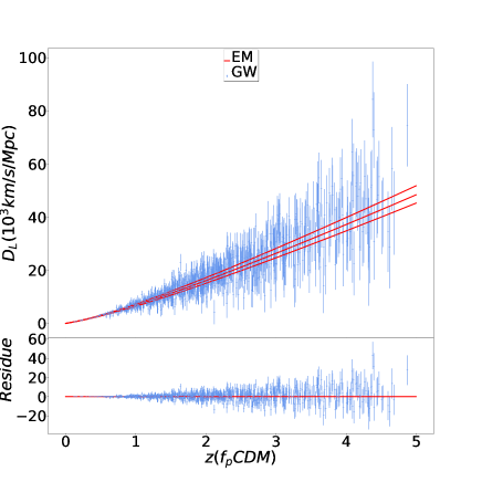
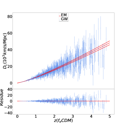
Figure 1: The data with error-bar are the simulated GW data. The red lines are the best fitted values and the $1\sigma$ errors from the EM fitting results. Specifically, the left panel is for the $f_{p}$CDM model, while the right panel is for the $f_{e}$CDM model.

Table 1: Best fitted values with $1\sigma$ and $2\sigma$ standard errors for the GW, EW and GW $+$ EM (combined) data for the $f_{e}$CDM and $f_{p}$CDM models.

$f_{p}CDM$	$\Omega_{m0}$	$H_{0}(km/s/Mpc)$	$b$	$\beta_{T}$	$w_{eff}$
GW	$0.263^{+0.048+0.068}_{-0.021-0.089}$	$68.21^{+1.32+2.51}_{-1.32-2.61}$	$-0.122^{+0.624+0.868}_{-0.361-1.023}$	$-0.018^{+0.131+0.152}_{-0.032-0.241}$	$-1.003^{+0.095+0.239}_{-0.146-0.212}$	$2.69\sigma$
EM	$0.293^{+0.010+0.020}_{-0.010-0.019}$	$68.41^{+1.23+2.44}_{-1.24-2.41}$	$-0.071^{+0.095+0.171}_{-0.078-0.182}$	$0.012^{+0.017+0.031}_{-0.015-0.033}$	$-1.018^{+0.024+0.047}_{-0.024-0.046}$	$2.67\sigma$
GW$+$Pantheon	$0.197^{+0.047+0.075}_{-0.038-0.083}$	$67.62^{+0.50+0.99}_{-0.50-0.97}$	$0.441^{+0.240+0.349}_{-0.151-0.382}$	$-0.151^{+0.120+0.171}_{-0.061-0.196}$	$-0.861^{+0.070+0.131}_{-0.070-0.131}$	$4.01\sigma$
GW$+$H(z)	$0.262^{+0.020+0.034}_{-0.036-0.014}$	$68.20^{+0.65+1.31}_{-0.65-1.31}$	$0.031^{+0.219+0.395}_{-0.178-0.410}$	$-0.014^{+0.052+0.081}_{-0.031-0.092}$	$-0.987^{+0.050+0.110}_{-0.061-0.110}$	$3.46\sigma$
GW$+$BAO	$0.274^{+0.016+0.031}_{-0.016-0.032}$	$68.40^{+0.63+1.21}_{-0.63-1.21}$	$-0.161^{+0.261+0.412}_{-0.170-0.458}$	$0.022^{+0.038+0.066}_{-0.030-0.070}$	$-1.034^{+0.051+0.099}_{-0.051-0.101}$	$3.30\sigma$
GW$+$CMBR	$0.277^{+0.009+0.019}_{-0.009-0.018}$	$68.61^{+0.57+1.12}_{-0.57-1.12}$	$-0.226^{+0.119+0.203}_{-0.090-0.218}$	$0.036^{+0.014+0.028}_{-0.014-0.029}$	$-1.052^{+0.022+0.043}_{-0.022-0.044}$	$3.21\sigma$
GW$+$Pantheon$+$H(z)	$0.258^{+0.020+0.035}_{-0.016-0.037}$	$67.77^{+0.50+0.98}_{-0.50-0.98}$	$0.141^{+0.159+0.292}_{-0.141-0.310}$	$-0.037^{+0.047+0.074}_{-0.030-0.083}$	$-0.956^{+0.043+0.097}_{-0.088-0.050}$	$3.90\sigma$
GW$+$Pantheon$+$BAO	$0.269^{+0.013+0.027}_{-0.013-0.026}$	$67.82^{+0.46+0.90}_{-0.46-0.90}$	$0.042^{+0.110+0.211}_{-0.110-0.279}$	$-0.009^{+0.018+0.050}_{-0.014-0.053}$	$-0.989^{+0.020+0.065}_{-0.072-0.024}$	$3.90\sigma$
GW$+$BAO$+$CMBR	$0.280^{+0.009+0.017}_{-0.009-0.016}$	$68.51^{+0.57+1.12}_{-0.57-1.12}$	$-0.223^{+0.118+0.221}_{-0.099-0.221}$	$0.035^{+0.016+0.029}_{-0.014-0.032}$	$-1.052^{+0.023+0.048}_{-0.023-0.045}$	$3.28\sigma$
GW $+$EM	$0.286^{+0.007+0.015}_{-0.007-0.014}$	$68.06^{+0.46+0.90}_{-0.46-0.89}$	$-0.117^{+0.086+0.152}_{-0.070-0.160}$	$0.020^{+0.013+0.025}_{-0.013-0.026}$	$-1.030^{+0.019+0.038}_{-0.019-0.038}$	$3.73\sigma$
$f_{e}CDM$	$\Omega_{m0}$	$H_{0}(km/s/Mpc)$	$b$	$\beta_{T}$	$w_{eff}$	Tension
GW	$0.261^{+0.028+0.040}_{-0.015-0.050}$	$67.46^{+0.78+1.33}_{-0.64-1.38}$	$b<0.404<0.708$	$-0.249^{+0.235+0.251}_{+0.046-0.41}$	$-0.869^{+0.034+0.231}_{-0.125-0.154}$	$3.88\sigma$
EM	$0.296^{+0.010+0.020}_{-0.010-0.019}$	$67.71^{+1.11+2.10}_{-1.11-2.09}$	$b<0.162<0.251$	$-0.031^{+0.028+0.031}_{-0.013-0.042}$	$-0.959^{+0.014+0.050}_{-0.041-0.042}$	$3.21\sigma$
GW$+$Pantheon	$0.269^{+0.023+0.035}_{-0.014-0.041}$	$67.58^{+0.50+0.97}_{-0.50-0.99}$	$0.261^{+0.154+0.261}_{-0.168-0.261}$	$-0.093^{+0.072+0.090}_{-0.041-0.169}$	$-0.906^{+0.032+0.11}_{-0.091-0.095}$	$4.03\sigma$
GW$+$H(z)	$0.276^{+0.011+0.021}_{-0.011-0.023}$	$67.68^{+0.71+1.11}_{-0.52-1.27}$	$b<0.282<0.432$	$-0.061^{+0.412+0.750}_{-0.411-0.644}$	$-0.923^{+0.022+0.092}_{-0.075-0.077}$	$3.84\sigma$
GW$+$BAO	$0.280^{+0.012+0.023}_{-0.012-0.023}$	$67.67^{+0.60+1.03}_{-0.47-1.08}$	$b<0.225<0.372$	$-0.048^{+0.063+0.121}_{-0.148-0.077}$	$-0.941^{+0.017+0.080}_{-0.059-0.060}$	$3.93\sigma$
GW$+$CMBR	$0.292^{+0.010+0.019}_{-0.010-0.018}$	$67.55^{+0.43+0.82}_{-0.43-0.88}$	$b<0.145<0.233$	$-0.028^{+0.027+0.028}_{-0.009-0.036}$	$-0.963^{+0.012+0.046}_{-0.036-0.037}$	$4.13\sigma$
GW$+$Pantheon$+$H(z)	$0.278^{+0.011+0.020}_{-0.010-0.023}$	$67.70^{+0.51+0.92}_{-0.46-0.99}$	$0.211^{+0.128+0.168}_{-0.114-0.211}$	$-0.058^{+0.056+0.058}_{-0.024-0.065}$	$-0.929^{+0.041+0.069}_{-0.047-0.071}$	$3.96\sigma$
GW$+$Pantheon$+$BAO	$0.282^{+0.012+0.021}_{-0.010-0.023}$	$67.64^{+0.45+0.86}_{-0.45-0.92}$	$b<0.220<0.338$	$-0.045^{+0.044+0.045}_{-0.013-0.058}$	$-0.944^{+0.020+0.065}_{-0.056-0.057}$	$4.04\sigma$
GW$+$BAO$+$CMBR	$0.292^{+0.009+0.018}_{-0.009-0.017}$	$67.54^{+0.42+0.78}_{-0.38-0.84}$	$b<0.142<0.230$	$-0.027^{+0.027+0.027}_{-0.008-0.036}$	$-0.964^{+0.011+0.045}_{-0.035-0.036}$	$4.16\sigma$
GW $+$ EM	$0.294^{+0.007+0.015}_{-0.007-0.014}$	$67.84^{+0.36+0.69}_{-0.36-0.74}$	$b<0.154<0.236$	$-0.029^{+0.026+0.029}_{-0.012-0.038}$	$-0.961^{+0.012+0.045}_{-0.038-0.039}$	$3.97\sigma$

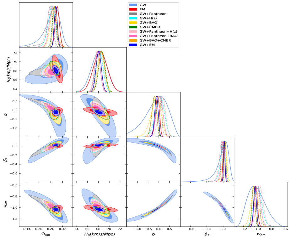
Figure 2: The probability density functions (pdfs) , the $68\%$ ($1\sigma$) and $95\%$ ($2\sigma$) confidence regions for the parameters ($\Omega_{m0}$, $H_{0}$, $b$, $\beta_{T}$ and $w_{e}ff$) in the $f_{p}$CDM model respectively.

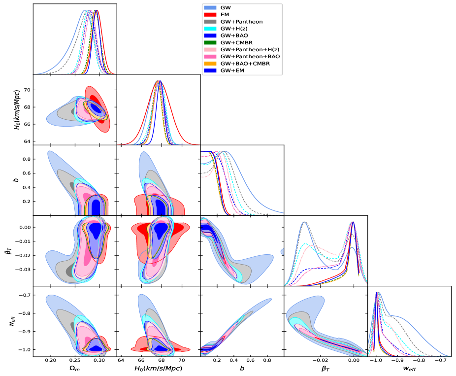
Figure 3: The probability density functions (pdfs) , the $68\%$ ($1\sigma$) and $95\%$ ($2\sigma$) confidence regions for the parameters ($\Omega_{m0}$, $H_{0}$, $b$, $\beta_{T}$ and $w_{e}ff$) in the $f_{e}$CDM model respectively.

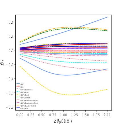
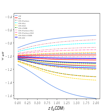
Figure 4: The evolution of $w_{eff}$ and $\beta_{T}$ of the $f_{p}$CDM model in $1\sigma$ region for the GW, EM and combined data separately.

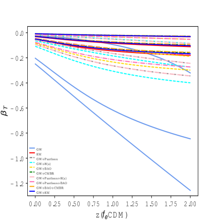
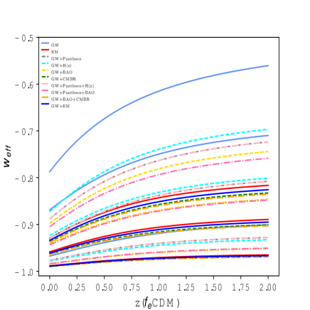
Figure 5: The evolution of $w_{eff}$ and $\beta_{T}$ of the $f_{e}$CDM model in $1\sigma$ region for the GW, EM and combined data separately.

4.3 Data Comparison

The Markov Chain Monte Carlo (MCMC) method Lewis:2002ah and the maximum likelihood method are used to constrain the $f(T)$ parameters. Firstly, we constrain the $f(T)$ models by using all the EM data (Pantheon$+$H(z)$+$BAO$+$CMBR). And we use the best fitted values of the results for EM data and ET design to simulate the GW data. We list the simulated GW data and the $1\sigma$ fitting results of EM data in Fig.1.

Comparing the best fitted value of GW data with its fiducial data, we could see the best fitted values of parameter $\Omega_{m0}$, $b$ and $H_{0}$ are smaller than the fiducial data. Meanwhile, $\beta_{T}$ is smaller the fiducial value and $w_{eff}$ is larger than the fiducial value. Furthermore, the constraining regions of $\Omega_{m0}$, $b$, $\beta_{T}$ and $w_{eff}$ given by GW constraint are much larger than that of the EM data. While that of GW data lead to a comparative constraint with the EM data for the $H_{0}$ parameter. Then, through the fiducial values are changed in the GW data, the best fitted values of all the parameters are still in the $1\sigma$ region of the EM constraining results. We calculate the residues by using the $1\sigma$ values to subtract the fiducial values. The residues have normal distributions which denote there is no evidence for a systematic difference between GW and EM-based estimated. Then, the simulated GW data are consistent with the EM data. And, the combinations of GW data with the EM data is reasonable.

As the $H_{0}$ tension is mainly between the early data and the late data, we consider three ways of combinations. Firstly, we combined GW with the Pantheon, H(z), BAO and CMBR data separately. Then we combined GW to the late measurements( Pantheon $+$ H(z)) and the early measurements ( BAO $+$CMBR) separately. And, the crossing combination (GW$+$BAO$+$Pantheon) is added as supplements. At last, we combined them all. To denote the $H_{0}$ problem, the data tension Raveri:2018wln is calculated

$$T_{1}(\theta)=\frac{|\theta(D_{1})-\theta(D_{2})|}{\sqrt{\sigma_{\theta}^{2}(D_{1})+\sigma_{\theta}^{2}(D_{2})}}$$ (16)

where $\theta$ is chosen as the best fitted values of $H_{0}$, the first data set $D_{1}$ is separately chosen as the three kinds of data discussed in the above, the second data is set as the SH0Es Teams data ($H_{0}=73.2\pm 1.3km/s/Mpc$ at $68\%$ confidence level) in this letter.

5 Constraining results

In Table 1, we show the constraining results of the constant parameters $\Omega_{m0}$, $H_{0}$, and $b$. Furthermore, we compute the evolving parameters $\beta_{T}$ and $w_{eff}$ as well. In Figs. 2 and 3 , we present the triangle plots of the parameters which include the probability density function (pdf) and the contours for both $f(T)$ models. In addition, we plot the $1\sigma$ evolutions of $\beta_{T}$ and $w_{eff}$ in Figs. 4 and 5 .

5.1 The $f_{p}$CDM model

The contours are closed and smooth and the pdfs are gaussian-distributed in $f_{p}$CDM model. Explicitly, either the EM or GW data alone can not distinguish the $f(T)$ model from the $\Lambda$CDM model. The constraining tendencies of GW$+$Pantheon and GW$+$H(z) data are similar which give out the positive best fitted $b$ and negative best fitted $\beta_{T}$. In the contrast, that of GW$+$BAO and GW$+$CMBR data are similar which give the negative best fitted $b$ and positive best fitted $\beta_{T}$. This is caused by the $H_{0}$ tension between the early and late EM data, and denotes the parameters $\beta_{T}$ and $b$ negatively related.

Because of the $H_{0}$ tension, the GW$+$Pantheon$+$H(z) and GW$+$BAO$+$CMBR both have tight constraining results. And the GW$+$BAO$+$CMBR data has the tightest constrain while the GW$+$EM one which includes all the EM data does not. The GW$+$Pantheon$+$BAO data has larger contours than the GW $+$Pantheon$+$H(z) and GW$+$BAO$+$CMBR data which denotes the $H_{0}$ tension as well. Obviously, the GW data combined with both the early and late EM data improve the constraint significantly. After the solution of the $H_{0}$ tension, the distinguishable problem will be more clear.

The $w_{eff}=0$ value is not included in $2\sigma$ regime for $f_{p}$CDM model by the constraining of the GW$+$BAO$+$CMBR data. In another saying, the $f_{p}$CDM model could be distinguished from $\Lambda$CDM in $2\sigma$ constraints by adding the GW data. The distinguishable effect is mainly from the $\beta_{T}$ parameter which is related to the GW luminosity data and breaks the main degeneration between the parameters.

5.2 The $f_{e}$CDM model

As shown in Table 1, we obtain a minus $\beta_{T}$ and a quintessence-like $w_{eff}$ in $f_{e}$CDM model as the setting of the prior $b>0$. The evolutions of $w_{eff}$ and $\beta_{T}$ almost follow $\Lambda$CDM model at late time which are quite flat. The contours of $\beta_{T}$ have two peaks for $f_{e}$CDM model. There is a non-gaussian behavior for $b$ which is caused by the prior $b>0$. Though the contours related to $b$ are not closed, but the contours related to $w_{eff}$ and $\beta_{T}$ are nearly closed.

Generally, the GW$+$Pantheon data constrains the $b$ parameter more effectively in the $f_{e}$CDM model. And, the best fitted value of all the data of the $\beta_{T}$ and $w_{eff}$ are close to $\Lambda$CDM model. As we set the $b>0$ prior for $f_{e}$CDM model, it does not face to the distinguishable problem.

5.3 Short summary

Comparing the constraining results for $f_{p}$CDM and $f_{e}$CDM models, the $1\sigma$ constraining regions of all the GW related data of $f_{e}$CDM model are comparable with that of $f_{p}$CDM model. The constraining precisions do not sensitive to the prior $b>0$. And the shape of the $f(T)$ function almost does not affect the constraining precision as well. And considering the tension between our data and the SH0Es data as list in Table 1, the combined data have larger tensions than the GW or EM data, that is mainly because the precision of the data are improved, while the shift of the best-fitted value is slight.

Finally, as shown in Figs. 4 and 5, at high $z$, the deviations from $\Lambda$CDM model become evident. Then more high $z$ data may help to distinguish them.

6 Conclusion

In this paper, we focused on the detection ability of the future GW data to constrain the $f(T)$ models and discussed the related $H_{0}$ tension problem. The GW$+$BAO$+$CMBR data give the tightest constraints. The GW data are powerful probes to distinguish the modified gravity from the GR, especially the degenerated ones in view of early EM data. As our computations show, the gravitational wave detections offer a remarkable approach to explore the universe from a new perspective, providing an access to astrophysical processes that are completely ignorant to EM observations.

Acknowledgments. YZ thanks Dr. Jingzhao Qi, Prof. Hao Wei, Dr. Tao Yang, Prof.Wen Zhao, YZ is supported by National Natural Science Foundation of China under Grant No.11905023, CQ CSTC under grant cstc2020jcyj-msxmX0810 and cstc2020jcyj-msxmX0555. HZ is supported by Shandong Province Natural Science Foundation under grant No. ZR201709220395, and the National Key Research and Development Program of China (No. 2020YFC2201400).

References

- (1) B. P. Abbott et al. [LIGO Scientific and Virgo Collaborations], Phys. Rev. Lett. 116, no. 6, 061102 (2016) doi:10.1103/PhysRevLett.116.061102 [arXiv:1602.03837 [gr-qc]].
- (2) B. P. Abbott et al. [LIGO Scientific and Virgo Collaborations], Phys. Rev. Lett. 116, no. 24, 241103 (2016) doi:10.1103/PhysRevLett.116.241103 [arXiv:1606.04855 [gr-qc]].
- (3) B. P. Abbott et al. [LIGO Scientific and Virgo Collaborations], Phys. Rev. X 6, no. 4, 041015 (2016) doi:10.1103/PhysRevX.6.041015 [arXiv:1606.04856 [gr-qc]].
- (4) B. P. Abbott et al. [LIGO Scientific and Virgo and 1M2H and Dark Energy Camera GW-E and DES and DLT40 and Las Cumbres Observatory and VINROUGE and MASTER Collaborations], Nature 551, no. 7678, 85 (2017) doi:10.1038/nature24471 [arXiv:1710.05835 [astro-ph.CO]].
- (5) B. P. Abbott et al. [LIGO Scientific and VIRGO Collaborations], Phys. Rev. Lett. 118, no. 22, 221101 (2017) doi:10.1103/PhysRevLett.118.221101 [arXiv:1706.01812 [gr-qc]].
- (6) B. P. Abbott et al. [LIGO Scientific and Virgo Collaborations], Phys. Rev. Lett. 119, no. 14, 141101 (2017) doi:10.1103/PhysRevLett.119.141101 [arXiv:1709.09660 [gr-qc]].
- (7) B. . P. .Abbott et al. [LIGO Scientific and Virgo Collaborations], Astrophys. J. 851, no. 2, L35 (2017) doi:10.3847/2041-8213/aa9f0c [arXiv:1711.05578 [astro-ph.HE]].
- (8) R. Abbott et al. [LIGO Scientific and Virgo], [arXiv:2010.14527 [gr-qc]].
- (9) R. Abbott et al. [LIGO Scientific, KAGRA and VIRGO], Astrophys. J. Lett. 915 (2021) no.1, L5 doi:10.3847/2041-8213/ac082e [arXiv:2106.15163 [astro-ph.HE]].
- (10) G. R. Bengochea and R. Ferraro, Phys. Rev. D 79, 124019 (2009) doi:10.1103/PhysRevD.79.124019 [arXiv:0812.1205 [astro-ph]].
- (11) E. V. Linder, Phys. Rev. D 81, 127301 (2010) Erratum: [Phys. Rev. D 82, 109902 (2010)] doi:10.1103/PhysRevD.81.127301, 10.1103/PhysRevD.82.109902 [arXiv:1005.3039 [astro-ph.CO]].
- (12) P. Wu and H. W. Yu, Eur. Phys. J. C 71, 1552 (2011) doi:10.1140/epjc/s10052-011-1552-2 [arXiv:1008.3669 [gr-qc]].
- (13) Y. F. Cai, S. Capozziello, M. De Laurentis and E. N. Saridakis, Rept. Prog. Phys. 79, no. 10, 106901 (2016) doi:10.1088/0034-4885/79/10/106901 [arXiv:1511.07586 [gr-qc]].
- (14) M. Punturo et al., Class. Quant. Grav. 27 (2010), 194002 doi:10.1088/0264-9381/27/19/194002
- (15) B. S. Sathyaprakash, B. F. Schutz and C. Van Den Broeck, Class. Quant. Grav. 27, 215006 (2010) doi:10.1088/0264-9381/27/21/215006 [arXiv:0906.4151 [astro-ph.CO]].
- (16) W.R. Hu and Y.L. Wu Y-L, National Science Review 4(5) (2017) doi: 10.1093/nsr/nwx116
- (17) J. Luo et al. [TianQin], Class. Quant. Grav. 33, no.3, 035010 (2016) doi:10.1088/0264-9381/33/3/035010 [arXiv:1512.02076 [astro-ph.IM]].
- (18) https://sci.esa.int/web/lisa
- (19) P. A. R. Ade et al. [Planck Collaboration], Astron. Astrophys. 594, A13 (2016) doi:10.1051/0004-6361/201525830 [arXiv:1502.01589 [astro-ph.CO]].
- (20) P. Ade, N. Aghanim, C. Armitage-Caplan, M. Arnaud, M. Ashdown, F. Atrio-Barandela, J. Aumont, C. Bac- cigalupi, A. Banday, R. Barreiro, et al., Astronomy Astrophysics 571, A16 (2014)
- (21) R. Ferraro, AIP Conf. Proc. 1471, 103 (2012) doi:10.1063/1.4756821 [arXiv:1204.6273 [gr-qc]].
- (22) T. Clifton, P. G. Ferreira, A. Padilla and C. Skordis, Phys. Rept. 513, 1 (2012) doi:10.1016/j.physrep.2012.01.001 [arXiv:1106.2476 [astro-ph.CO]].
- (23) Y. Zhang, H. Li, Y. Gong and Z. H. Zhu, JCAP 1107, 015 (2011) doi:10.1088/1475-7516/2011/07/015 [arXiv:1103.0719 [astro-ph.CO]].
- (24) A. Awad, W. El Hanafy, G. G. L. Nashed and E. N. Saridakis, JCAP 1802, no. 02, 052 (2018) doi:10.1088/1475-7516/2018/02/052 [arXiv:1710.10194 [gr-qc]].
- (25) K. Bamba, C. Q. Geng and C. C. Lee, arXiv:1008.4036 [astro-ph.CO].
- (26) A. Paliathanasis, J. D. Barrow and P. G. L. Leach, Phys. Rev. D 94, no. 2, 023525 (2016) doi:10.1103/PhysRevD.94.023525 [arXiv:1606.00659 [gr-qc]].
- (27) K. Bamba, C. Q. Geng, C. C. Lee and L. W. Luo, JCAP 1101, 021 (2011) doi:10.1088/1475-7516/2011/01/021 [arXiv:1011.0508 [astro-ph.CO]].
- (28) S. B. Nassur, M. J. S. Houndjo, I. G. Salako and J. Tossa, arXiv:1601.04538 [physics.gen-ph].
- (29) I. G. Salako, M. E. Rodrigues, A. V. Kpadonou, M. J. S. Houndjo and J. Tossa, JCAP 1311, 060 (2013) doi:10.1088/1475-7516/2013/11/060 [arXiv:1307.0730 [gr-qc]].
- (30) S. Nesseris, S. Basilakos, E. N. Saridakis and L. Perivolaropoulos, Phys. Rev. D 88, 103010 (2013) doi:10.1103/PhysRevD.88.103010 [arXiv:1308.6142 [astro-ph.CO]].
- (31) R. C. Nunes, S. Pan and E. N. Saridakis, JCAP 1608, no. 08, 011 (2016) doi:10.1088/1475-7516/2016/08/011 [arXiv:1606.04359 [gr-qc]].
- (32) R. C. Nunes, JCAP 1805, no. 05, 052 (2018) doi:10.1088/1475-7516/2018/05/052 [arXiv:1802.02281 [gr-qc]].
- (33) S. Basilakos, S. Nesseris, F. K. Anagnostopoulos and E. N. Saridakis, JCAP 08 (2018), 008 doi:10.1088/1475-7516/2018/08/008 [arXiv:1803.09278 [astro-ph.CO]].
- (34) W. S. Zhang, C. Cheng, Q. G. Huang, M. Li, S. Li, X. D. Li and S. Wang, Sci. China Phys. Mech. Astron. 55, 2244 (2012) doi:10.1007/s11433-012-4945-9 [arXiv:1202.0892 [astro-ph.CO]].
- (35) S. Capozziello, O. Luongo, R. Pincak and A. Ravanpak, Gen. Rel. Grav. 50, no. 5, 53 (2018) doi:10.1007/s10714-018-2374-4 [arXiv:1804.03649 [gr-qc]].
- (36) R. C. Nunes, S. Pan and E. N. Saridakis, Phys. Rev. D 98, no. 10, 104055 (2018) doi:10.1103/PhysRevD.98.104055 [arXiv:1810.03942 [gr-qc]].
- (37) R. C. Nunes, M. E. S. Alves and J. C. N. de Araujo, arXiv:1905.03237 [gr-qc].
- (38) J. Z. Qi, S. Cao, M. Biesiada, X. Zheng and H. Zhu, Eur. Phys. J. C 77, no. 8, 502 (2017) doi:10.1140/epjc/s10052-017-5069-1 [arXiv:1708.08603 [astro-ph.CO]].
- (39) S. F. Yan, P. Zhang, J. W. Chen, X. Z. Zhang, Y. F. Cai and E. N. Saridakis, Phys. Rev. D 101 (2020) no.12, 121301 doi:10.1103/PhysRevD.101.121301 [arXiv:1909.06388 [astro-ph.CO]].
- (40) N. Aghanim et al. [Planck], Astron. Astrophys. 641, A6 (2020) doi:10.1051/0004-6361/201833910 [arXiv:1807.06209 [astro-ph.CO]].
- (41) A. G. Riess, S. Casertano, W. Yuan, J. B. Bowers, L. Macri, J. C. Zinn and D. Scolnic, Astrophys. J. Lett. 908, no.1, L6 (2021) doi:10.3847/2041-8213/abdbaf [arXiv:2012.08534 [astro-ph.CO]].
- (42) E. Di Valentino, O. Mena, S. Pan, L. Visinelli, W. Yang, A. Melchiorri, D. F. Mota, A. G. Riess and J. Silk, [arXiv:2103.01183 [astro-ph.CO]].
- (43) K. Bamba, S. Capozziello, M. De Laurentis, S. Nojiri and D. Sa´ez-Go´mez, Phys. Lett. B 727, 194 (2013) doi:10.1016/j.physletb.2013.10.022 [arXiv:1309.2698 [gr-qc]].
- (44) Y. F. Cai, C. Li, E. N. Saridakis and L. Xue, Phys. Rev. D 97, no. 10, 103513 (2018) doi:10.1103/PhysRevD.97.103513 [arXiv:1801.05827 [gr-qc]].
- (45) H. Abedi and S. Capozziello, Eur. Phys. J. C 78, no. 6, 474 (2018) doi:10.1140/epjc/s10052-018-5967-x [arXiv:1712.05933 [gr-qc]].
- (46) T. Baker, E. Bellini, P. G. Ferreira, M. Lagos, J. Noller and I. Sawicki, Phys. Rev. Lett. 119, no. 25, 251301 (2017) doi:10.1103/PhysRevLett.119.251301 [arXiv:1710.06394 [astro-ph.CO]].
- (47) J. M. Ezquiaga and M. Zumalacárregui, Phys. Rev. Lett. 119 (2017) no.25, 251304 doi:10.1103/PhysRevLett.119.251304 [arXiv:1710.05901 [astro-ph.CO]].
- (48) D. E. Holz and S. A. Hughes, Astrophys. J. 629, 15 (2005) doi:10.1086/431341 [astro-ph/0504616].
- (49) B.F. Schutz, 1986, Nature, 323, 310
- (50) E. Belgacem, Y. Dirian, S. Foffa and M. Maggiore, Phys. Rev. D 97, no. 10, 104066 (2018) doi:10.1103/PhysRevD.97.104066 [arXiv:1712.08108 [astro-ph.CO]].
- (51) E. Belgacem et al. [LISA Cosmology Working Group], arXiv:1906.01593 [astro-ph.CO].
- (52) L. Amendola, I. Sawicki, M. Kunz and I. D. Saltas, JCAP 1808 (2018) 030 doi:10.1088/1475-7516/2018/08/030 [arXiv:1712.08623 [astro-ph.CO]].
- (53) M. Lagos, M. Fishbach, P. Landry and D. E. Holz, Phys. Rev. D 99, no. 8, 083504 (2019) doi:10.1103/PhysRevD.99.083504 [arXiv:1901.03321 [astro-ph.CO]].
- (54) G. Calcagni, S. Kuroyanagi, S. Marsat, M. Sakellariadou, N. Tamanini and G. Tasinato, arXiv:1904.00384 [gr-qc].
- (55) Extracting Physics from Gravitational Waves: Testing the Strong-field Dynamics of General Relativity and Inferring the Large-scale Structure of the Universe,Authors: Li, Tjonnie G. F. 2015, Springer Theses
- (56) W. Zhao, C. Van Den Broeck, D. Baskaran and T. G. F. Li, Phys. Rev. D 83, 023005 (2011) doi:10.1103/PhysRevD.83.023005 [arXiv:1009.0206 [astro-ph.CO]].
- (57) R. G. Cai and T. Yang, Phys. Rev. D 95, no. 4, 044024 (2017) doi:10.1103/PhysRevD.95.044024 [arXiv:1608.08008 [astro-ph.CO]].
- (58) D. M. Scolnic, D. O. Jones, A. Rest, Y. C. Pan, R. Chornock, R. J. Foley, M. E. Huber, R. Kessler, G. Narayan and A. G. Riess, et al. Astrophys. J. 859, no.2, 101 (2018) doi:10.3847/1538-4357/aab9bb [arXiv:1710.00845 [astro-ph.CO]].
- (59) C. Zhang, H. Zhang, S. Yuan, T. J. Zhang and Y. C. Sun, Res. Astron. Astrophys. 14, no. 10, 1221 (2014) doi:10.1088/1674-4527/14/10/002 [arXiv:1207.4541 [astro-ph.CO]].
- (60) R. Jimenez, L. Verde, T. Treu and D. Stern, Astrophys. J. 593, 622 (2003) doi:10.1086/376595 [astro-ph/0302560].
- (61) M. Moresco, L. Verde, L. Pozzetti, R. Jimenez and A. Cimatti, JCAP 1207, 053 (2012) doi:10.1088/1475-7516/2012/07/053 [arXiv:1201.6658 [astro-ph.CO]].
- (62) M. Moresco, Mon. Not. Roy. Astron. Soc. 450, no. 1, L16 (2015) doi:10.1093/mnrasl/slv037 [arXiv:1503.01116 [astro-ph.CO]].
- (63) E. Gaztanaga, A. Cabre and L. Hui, Mon. Not. Roy. Astron. Soc. 399, 1663 (2009) doi:10.1111/j.1365-2966.2009.15405.x [arXiv:0807.3551 [astro-ph]].
- (64) J. Simon, L. Verde and R. Jimenez, Phys. Rev. D 71, 123001 (2005) doi:10.1103/PhysRevD.71.123001 [astro-ph/0412269].
- (65) C. H. Chuang and Y. Wang, Mon. Not. Roy. Astron. Soc. 426, 226 (2012) doi:10.1111/j.1365-2966.2012.21565.x [arXiv:1102.2251 [astro-ph.CO]].
- (66) X. Xu, A. J. Cuesta, N. Padmanabhan, D. J. Eisenstein and C. K. McBride, Mon. Not. Roy. Astron. Soc. 431, 2834 (2013) doi:10.1093/mnras/stt379 [arXiv:1206.6732 [astro-ph.CO]].
- (67) M. Moresco et al., JCAP 1605, no. 05, 014 (2016) doi:10.1088/1475-7516/2016/05/014 [arXiv:1601.01701 [astro-ph.CO]].
- (68) C. Blake et al., Mon. Not. Roy. Astron. Soc. 425, 405 (2012) doi:10.1111/j.1365-2966.2012.21473.x [arXiv:1204.3674 [astro-ph.CO]].
- (69) D. Stern, R. Jimenez, L. Verde, M. Kamionkowski and S. A. Stanford, JCAP 1002, 008 (2010) doi:10.1088/1475-7516/2010/02/008 [arXiv:0907.3149 [astro-ph.CO]].
- (70) L. Samushia et al., Mon. Not. Roy. Astron. Soc. 429, 1514 (2013) doi:10.1093/mnras/sts443 [arXiv:1206.5309 [astro-ph.CO]].
- (71) N. G. Busca et al., Astron. Astrophys. 552, A96 (2013) doi:10.1051/0004-6361/201220724 [arXiv:1211.2616 [astro-ph.CO]].
- (72) A. Font-Ribera et al. [BOSS Collaboration], JCAP 1405, 027 (2014) doi:10.1088/1475-7516/2014/05/027 [arXiv:1311.1767 [astro-ph.CO]].
- (73) T. Delubac et al. [BOSS Collaboration], Astron. Astrophys. 574, A59 (2015) doi:10.1051/0004-6361/201423969 [arXiv:1404.1801 [astro-ph.CO]].
- (74) W. J. Percival et al. [SDSS Collaboration], Mon. Not. Roy. Astron. Soc. 401, 2148 (2010) doi:10.1111/j.1365-2966.2009.15812.x [arXiv:0907.1660 [astro-ph.CO]].
- (75) C. Blake et al., Mon. Not. Roy. Astron. Soc. 418, 1707 (2011) doi:10.1111/j.1365-2966.2011.19592.x [arXiv:1108.2635 [astro-ph.CO]].
- (76) F. Beutler et al., Mon. Not. Roy. Astron. Soc. 416, 3017 (2011) doi:10.1111/j.1365-2966.2011.19250.x [arXiv:1106.3366 [astro-ph.CO]].
- (77) A. Lewis and S. Bridle, Phys. Rev. D 66, 103511 (2002) doi:10.1103/PhysRevD.66.103511 [astro-ph/0205436].
- (78) M. Raveri and W. Hu, Phys. Rev. D 99 (2019) no.4, 043506 doi:10.1103/PhysRevD.99.043506 [arXiv:1806.04649 [astro-ph.CO]].