Gravitational Waves and Primordial Black Holes from
Supersymmetric Hybrid Inflation

Vassilis C. Spanos and Ioanna D. Stamou

National and Kapodistrian University of Athens, Department of Physics,
Section of Nuclear & Particle Physics, GR–15784 Athens, Greece

We study the effect of supergravity corrections due to a linear and a squared term in the Kähler potential, in the context of a supersymmetric hybrid inflation model. By appropriate choice of the parameters associated to these terms, we are able to satisfy the main cosmological constraints for the spectral index $n_{s}$ and the tensor-to-scalar ratio $r$. In addition, this model predicts primordial black hole abundance enough to account for the whole dark matter of the Universe and gravitational wave spectra within the reach of future detection experiments. The predictions of the model can be made compatible to the NANOGrav reported signal, at the cost of significantly lower primordial black hole abundance.

1 Introduction

An important milestone in Cosmology was the detection of Gravitational Waves (GWs) by LIGO and Virgo collaborations [1, 2, 3]. The detection of such signals, related to the merging of black holes or neutron stars, triggered numerous studies, exploring the possibility that the primordial black holes (PBHs) constitute a significant part or the whole of the Dark Matter (DM) of the Universe. In addition, recently, it was reported strong evidence for stochastic common-spectrum process by the NANOGrav collaboration [4, 5, 6]. Needless to say, that analogous and more precise detection signals for GWs are expected from future space-based GW interferometers such as LISA, BBO, DECIGO, SKA and Tianquin,[7, 8, 9, 10, 11, 12].

As a result, many theoretical studies have appeared in the literature [13, 14, 15, 16, 17, 18, 19, 20, 21, 22, 23, 24, 25, 26, 27, 29, 28, 30, 31, 32, 33, 34, 35, 36, 37, 38, 39, 40], which explain the production of PBH as a fraction of DM of the Universe. This PBH production during the radiation dominance epoch, can be associated to a significant enhancement of the scalar power spectrum. Many of these models are based on single field inflation and especially on models with a near inflection point in the effective scalar potential [13, 14, 15, 16, 17, 18, 19, 20, 21, 22]. The required enhancement factor of the power spectrum is calculated to be seven order of magnitudes [13, 14, 15, 16, 17, 18, 19, 20, 21, 22]. A severe drawback of these models, is the high level of the necessary fine-tuning, in order to achieve such a big amplification of the power spectrum. For this reason, alternative methods have been proposed to alleviate the issue of the fine-tuning, for example the multi-field inflation models [25, 26, 27, 29, 28, 30] or models with a step behavior in the effective scalar potential[41, 42, 23, 24].

In this paper we follow a different avenue in order to explain the generation of GWs and the production of PBHs. Specifically, we study the case of a hybrid inflation model [43, 44], including supergravity (SUGRA) corrections. The main advantage of the hybrid models, is that the required fine-tuning is significantly smaller than in models where the PBHs are produced due to an inflection point in the scalar potential. The characteristic feature of a hybrid model, is that the minimum of the scalar effective potential corresponds to the false vacuum with non-vanishing energy density [43, 45]. This false vacuum dominates and becomes unstable, when the inflaton field acquires a critical value[45]. Needless to say, that the inflationary predictions from the hybrid false vacuum models are quite different than the true vacuum models. Specifically, in the true vacuum models inflation ends with oscillations in the minimum of the potential, which designate the reheating. Moreover, it appears that the inflation scale in true vacuum models differs from this in the false vacuum. In particular, in the false vacuum models inflation occurs far below the Planck scale, therefore they are similar to the embedded SUGRA models [45]. On the contrary, the inflation scale in the true vacuum models is predicted to be usually high.

The main drawback of hybrid inflationary models was their prediction for the spectral index $n_{s}\gtrsim 1$  [45, 46, 47], value excluded by the Planck data [48, 49]. In [50, 51] introduced one-loop radiative corrections in order to achieve a reduction to $n_{s}$, although during the last years alternative methods have been proposed [52, 53, 54, 55, 56, 57, 58, 59, 60, 61, 62, 63, 64, 65]. Specifically, in the context of no-scale SUGRA hybrid models, a reduced value for $n_{s}$ can be predicted [66, 67, 68]. In the context of hybrid models the production of PBHs has already be studied [69, 70, 71, 72], also with small values for $n_{s}$. This PBH production obtained by an appropriate enhancement of the power spectrum of the scalar perturbations. In addition, the production of GWs can be obtained by this enhancement [73, 74, 75, 76, 77, 78, 79, 80, 81].

In this work we present a pure hybrid model, where we achieve cosmologically accepted values for $n_{s}<1.0$ due to SUGRA corrections. These corrections are related to a linear and a squared term, added in the Kähler potential. The enhancement of the power spectrum in hybrid models, such as shown in Ref. [70], occurs during the mild waterfall phase. Specifically, these models are based on a two-field inflation scenario, where one field acquires tachyonic solution in the critical point and the other, which plays the role of the inflaton, becomes unstable. Thus, the analysis of the background dynamics is decomposed in two phases: a slow-roll phase until the critical point and a second waterfall phase till the end of the inflation. The evaluation of the inflationary observables during these phases has been performed analytically in the slow-roll approximation [70, 82]. For comparison we have performed also a numerical solution of the background equations as well as the perturbations.

In the context of our model we have chose two representative sets of parameters for the extra Kähler terms. In any case we are able to satisfy the main cosmological constraints for the spectral index $n_{s}$ and the tensor-to-scalar ratio $r$. Moreover, this model predicts PBH abundance enough to account for the total DM of the Universe and GW spectra that can be detected in the future experiments like LISA, DELIGO etc. With an appropriate choice of the parameters, the GW spectrum can be made compatible to NANOGrav signal, but in this case the PBH abundance is much smaller, due to the SUBARU constraints.

The layout of the paper is as follows: In Section 2 we introduce the hybrid model with the SUGRA correction as discussed before, in order to derive acceptable values for the spectral index $n_{s}$ and the tensor-to-scalar ratio $r$. In Section 3 we present the background dynamics of the waterfall as well as the perturbation of the fields. We calculate analytically the scalar power spectrum based on the slow-roll approximation and for comparison we evaluate also the spectrum using a numerical solution. In Section 4 we evaluate the energy density of the GWs and we show that the model yields detectable spectra for the future experiments, like LISA, but also can explain the reported signal from the NANOGrav collaboration. In Section 5 we evaluate the fractional abundance of PBHs, which for a particular choice of the parameters, can account for the whole DM of the Universe. Furthermore, in Section 6 we estimate the amount of the required fine-tuning and we present our concluding remarks.

2 The Hybrid Model

The hybrid model [43, 45, 50] results from the globally supersymmetric renormalizable superpotential

$$W=\kappa\,S(\Psi_{1}{\Psi}_{2}-m^{2})\,,$$ (2.1)

where $\Psi_{1},\Psi_{2}$ are chiral superfields, the scalar component of the superfield, $S$ is the gauge singlet inflaton field, $\kappa$ is a dimensionless coupling constant and $m$ is a mass. It is important to notice that this superpotential is symmetric under $R$-symmetry, or in other words, transformations of the field such as $X\rightarrow e^{i\omega}X$ lead to the transformation of the superpotential $W\rightarrow e^{i\omega}W$. This symmetry removes the undesirable self-couplings of the inflaton field $S$, and it is the only symmetry which treats the false vacuum in a natural way [50].

The scalar potential in SUSY is given from the following expression

$${V_{F}^{SUSY}=\sum_{i}\left|\frac{\partial W}{\partial F_{i}}\right|^{2}}$$ (2.2)

where $F_{i}$ indicates the superfields: $\Psi_{1},\Psi_{2}$ and $S$. In the case of superpotential (2.1), one gets we have:

$${V_{F}^{SUSY}=\left|\kappa(\Psi_{1}{\Psi}_{2}-m^{2})\right|^{2}+\left|\kappa S\Psi_{1}\right|^{2}+\left|\kappa S{\Psi}_{2}\right|^{2}}$$ (2.3)

We consider the following form of the Kähler potential:

$$K=S\bar{S}+\Psi_{1}{\bar{\Psi}_{1}}+\Psi_{2}{\bar{\Psi}_{2}}$$ (2.4)

For the choice of Eq. (2.4) we have the following Kähler metric

$${K_{i\bar{j}}=\frac{\partial^{2}K}{\partial F^{i}\partial{F}^{\bar{j}}}=\begin{pmatrix}1&0&0\\ 0&1&0\\ 0&0&1\\ \end{pmatrix}.}$$ (2.5)

So the kinetic term of the Langrangian is given

$${L_{kin}={K_{i\bar{j}}\partial_{\mu}F^{i}\partial^{\mu}F^{\bar{j}}}}$$ (2.6)

Hence the scalar potential is given from

$${V_{F}^{\text{SUSY}}=\Lambda\left[\left(1-\frac{\psi^{2}}{M^{2}}\right)^{2}+\frac{2\phi^{2}\psi^{2}}{M^{4}}\right]}\,,$$ (2.7)

where we have assumed $\Lambda=\kappa^{2}m^{4}$ and $M^{2}\equiv 2m^{2}$. In order to fix the non-canonical kinetic term we have $|S|=\phi/\sqrt{2}$ and $|\Psi_{1}|=|\Psi_{2}|=\psi/\sqrt{2}$  [45, 56]. The potential is flat along the direction $\psi=0$, $|\phi|>|\phi_{c}|=m\sqrt{2}$ and is given by a constant value for the energy density $V=\kappa^{2}m^{4}$. One the other hand, the field $\psi$ develops tachyonic solutions if

$${\kappa^{2}(-2m^{2}+\phi^{2}+3\psi^{2})<0}\,,$$ (2.8)

Along the flat direction this condition becomes,

$${\phi^{2}<\phi_{c}^{2}=2m^{2}\equiv M^{2}}\,,$$ (2.9)

where $\phi_{c}$ is the critical value of the field $\phi$, after which this field $\psi$ becomes tachyonic. The main phenomenological issue of this model is that the predicted spectral index, $n_{s}$, is almost equal to unity, value rejected by the Planck data [48]. It has been proposed that incorporating the one-loop radiative corrections, leads to a red spectral index [50].

However, there is an alternative way to fix this problematic feature. By incorporating SUGRA corrections, one maintains the basic characteristics of the model, such as the waterfall behavior or the false vacuum inflation, and predicts $n_{s}\lesssim 1$. Specifically we consider a Kähler potential like

$$K=S\bar{S}+b_{1}(S+\bar{S})+b_{2}(S+\bar{S})^{2}+\Psi_{1}{\bar{\Psi}_{1}}+\Psi_{2}{\bar{\Psi}_{2}}\,$$ (2.10)

where $b_{1}$ is a dimensionful parameter with mass dimensions and $b_{2}$ is dimensionless. As for the origin of these parameters here we will remain agnostic, but their role and their phenomenologically preferred values will be discussed in the following. This form of Kähler potential is similar to Eq. (2.4) plus a shift-symmetric term  [83].

We calculate the $F$-term of the scalar potential using its general form is SUGRA models [84]

$$V_{F}^{\text{SUGRA}}=e^{K/{M_{P}}^{2}}\left[\left({K^{-1}}\right)^{i}_{\bar{j}}\left(W^{\bar{j}}+\frac{WK^{\bar{j}}}{{M_{P}}^{2}}\right)\left(\bar{W}_{i}+\frac{\bar{W}K_{i}}{{M_{P}}^{2}}\right)-\frac{3|W|^{2}}{{M_{P}}^{2}}\right]\,,$$ (2.11)

where $({K^{-1}})^{i}_{\bar{j}}$ is the inverse Kähler metric, $K_{i}=\frac{\partial K}{\partial F^{i}}$ and $W_{i}=\frac{\partial W}{\partial F^{i}}$. $M_{P}$ is the reduced Planck mass. The indices $i,j$ in this equation and thereafter, run over the chiral superfields $S$, $\Psi_{1}$ and $\Psi_{2}$ and with bar we denote the conjugate pair of each superfield. For the superpotential, we use the (2.1). In order to calculate the corrections in the effective scalar potential we expand the exponential in Eq. (2.11) as

$${e^{K/M_{P}^{2}}=1+\frac{K}{M_{P}^{2}}+\frac{K^{2}}{2\,M_{P}^{4}}+\mathcal{O}\left(\frac{1}{M_{P}^{6}}\right)\,.}$$ (2.12)

The Kähler metric for the Kähler potential (2.10) takes the form

$${K_{i\bar{j}}=\begin{pmatrix}1+2b_{2}&0&0\\ 0&1&0\\ 0&0&1\\ \end{pmatrix}}.$$ (2.13)

Using in (2.11), the Eqs. (2.1), (2.10), (2.12) and (2.13), the scalar potential reads as

$${V_{F}^{\text{SUGRA}}=\frac{\kappa^{2}(M^{4}-2M^{2}\psi^{2}+2\psi^{2}\phi^{2}+\psi^{4})}{4+8b_{2}}+\frac{\mathcal{A}_{1}}{M_{P}^{2}}+\frac{\mathcal{A}_{2}}{M_{P}^{4}}+\mathcal{O}\left(\frac{1}{M_{P}^{6}}\right)}\,,$$ (2.14)

where we have assumed that $|\Psi_{1}|=|\Psi_{2}|=\psi/\sqrt{2}$, as before. For the superfield $S$, we need to fix the non-canonical kinetic term by considering the Kähler metric in Eq. (2.13). Hence we have considered the following redefinition of the field

$$S=\frac{\phi}{\sqrt{2+4b_{2}}}\,.$$ (2.15)

The $\mathcal{A}_{1,2}$ are functions of $M,\phi,\psi$ with mass dimensions 6 and 8, respectively. Detailed expression for these can be found in Appendix A in Eqs. (A.7) and (A.8). One can notice that the first term in (2.14) is $V_{F}^{\text{SUSY}}/(1+2b_{2})$. In the limit $M_{P}\rightarrow\infty$ and $b_{2}\rightarrow 0$ apparently one derives the SUSY potential as in Eq. (2.7).

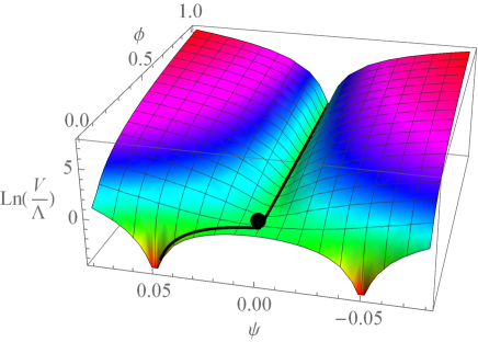
Figure 1: The quantity $\ln\left(\frac{V}{\Lambda}\right)$, using Eq. (2.16) with $b_{1}=3.506\times 10^{-4}\,M_{P}$, $b_{2}=-3.5\times 10^{-3}$ and $m=0.05\,M_{P}$. The fields $\phi$ and $\psi$ are measured in $M_{P}$ units. The black bullet denotes the position of the critical point.

Therefore, the total effective scalar potential is

$$V\equiv V_{F}^{\text{SUGRA}}=\Lambda\left[\left(1-\frac{\psi^{2}}{M^{2}}\right)^{2}+\frac{2\phi^{2}\psi^{2}}{M^{4}}+\tilde{V}_{F}^{\text{correction}}\right],$$ (2.16)

where $V_{F}^{\text{correction}}=V_{F}^{\text{SUGRA}}-V_{F}^{\text{SUSY}}$ from Eqs. (2.7) and (2.14) and $\tilde{V}_{F}^{\text{correction}}=V_{F}^{\text{correction}}/\Lambda$. If we expand this expression around the critical value of $\phi$ we derive[70, 85]

$$\tilde{V}_{F}^{\text{correction}}=a_{0}+a_{1}(\phi-\phi_{c})+a_{2}(\phi-\phi_{c})^{2}+a_{3}(\phi-\phi_{c})^{3}+a_{4}(\phi-\phi_{c})^{4}.$$ (2.17)

In this expansion, terms up to $a_{2}$ are related to $\mathcal{A}_{1}$ in (2.14), where these up to $a_{4}$ are related to $\mathcal{A}_{2}$. The numerical calculation reveals that the terms which appear in (2.14), suffice to approximate the $V_{F}^{\text{SUGRA}}$ in (2.11). More details can be found in the Appendix.

In Fig. 1 we present the effective scalar potential in Eq. (2.16). As one can notice, the inflaton field moves through the valley until it reaches the critical point. After that the other field, which is called waterfall, acquires tachyonic solution and the inflaton moves through the waterfall. Finally, the inflation ends in false vacuum. We can show that the prediction of the $n_{s}$ in this model is indeed compatible with the Planck cosmological data. In the slow-roll limit it is known that

$$n_{s}=1+2\eta_{V}-6\epsilon_{V}\,,$$ (2.18)

with

$$\varepsilon_{V}=\frac{M_{P}^{2}}{2}\left(\frac{V^{\prime}}{V}\right)^{2},\quad\eta_{V}=M_{P}^{2}\,\frac{V^{\prime\prime}}{V}\,.$$ (2.19)

Prime denotes derivation with respect to the fields. It is worth noting that in this model we get $n_{s}=0.965$, consistent with the current data. For the tensor-to-scalar ratio we use the corresponding slow-roll expression

$$r=16\,\varepsilon_{V}\,.$$ (2.20)

Detailed phenomenological analysis delineating values for $b_{1,2}$ compatible with the experimental constraints for $n_{s}$ and $r$ will be discussed in the following section.

3 Background Dynamics And Perturbations Along The Waterfall

In the hybrid inflation models two scalar fields are required: the inflaton field $\phi$ and the waterfall field $\psi$. The field $\psi$ becomes tachyonic at some critical value $\phi=\phi_{c}$, where its mass squared gets negative values. In this section we discuss the background dynamics for both $\phi$ and $\psi$ fields. In addition, we present the evaluation of scalar power spectrum with analytical and numerical tools, adopting methods from Refs [70, 82].

Model	$M(M_{P})$	$b_{1}(10^{-4}M_{P})$	$b_{2}(10^{-3})$	$\Lambda(10^{-20}M_{P}^{4})$	$n_{s}$	$r$
set 1	$0.05$	${3.506}$	${-3.5}$	${4.9}$	${0.9651}$	${1.55\times 10^{-12}}$
set 2	$0.10$	$8.918$	$-5.0$	$140$	$0.9684$	$1.54\times 10^{-10}$

Table 1: The prediction for the spectral index $n_{s}$ and ratio tensor-to-scalar $r$ for two representative sets of the parameters $b_{1,2}$.

First we calculate the evolution of the fields with respect to the cosmic time, as described from the potential (2.16). Consequently, we evaluate the spectral index $n_{s}$ and the tensor-to-scalar ratio $r$ using the Eqs. (2.18) and (2.20), respectively. Our results for two sets for the parametres $b_{1,2}$ are shown in Table 1. We notice that the additional terms, that depend on $b_{1,2}$ are found to be numerically at least three orders of magnitude smaller than the dominant $M$-term. On the other hand, their presence is important in order to satisfy the cosmological constraints. This can be understood, because the subdominant terms contribute in the derivatives of the potential $V$ and through these to $n_{s}$. In Fig. 2 we plot these predictions for the observables $n_{s}$ and $r$ along with the current allowed regions by the Planck 2018 collaboration [48].

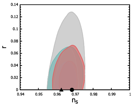
Figure 2: The predictions of our models for $n_{s}$ and $r$ plotted against the Planck 2018 constraints [48]. Triangle corresponds to set 1 and bullet to set 2, as given in Table 1.

The background dynamics is described by the Friedmann-Lemaître equation

$$H^{2}=\frac{1}{3M_{P}^{2}}\Big{(}\frac{\dot{\phi}^{2}}{2}+\frac{\dot{\psi}^{2}}{2}+V(\phi,\psi)\Big{)}$$ (3.1)

and the Klein-Gordon equations

$$\begin{split}\ddot{\phi}+3H\dot{\phi}+\frac{\partial V}{\partial\phi}=0\\ \ddot{\psi}+3H\dot{\psi}+\frac{\partial V}{\partial\psi}=0\,,\end{split}$$ (3.2)

where the dots denote differentiation with respect to cosmic time. In Fig. 3 we display the full solution of the (3.2) for the fields $\phi$ and $\psi$. As initial conditions for the solution we assume those of the critical point. Specifically, we assume $\phi_{ic}=\phi_{c}=0.05\,M_{P}$ and $\psi_{ic}=1.3\times 10^{-10}\,M_{P}$ and we calculate the background equations until the end of inflation, or equivalently until the parameter $\varepsilon=-\dot{H}/H^{2}$ reaches the value 1.

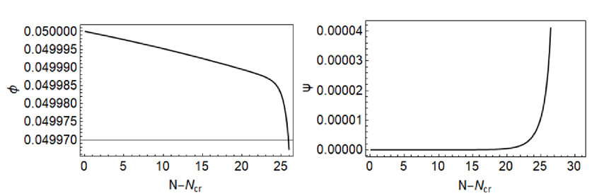
Figure 3: The fields $\phi$, $\psi$ as functions of the number of e-folds $N$ in $M_{P}$ units, starting from the critical point. We evaluate them solving the full background Eqs. (3.2) using the scalar potential (2.16).

The potential, we proposed in Eq. (2.16), gives significant enhancement in the power spectrum, almost by seven order of magnitude, due to the waterfall behavior, as it has been pointed out in [70]. In the following we present the analytical calculation of the power spectrum based on the slow-roll approximation and for comparison the corresponding numerical result based on the integration of curvature perturbations of the fields.

3.1 The slow-roll approximation

The equations of motion (3.2) can be solved numerically. However, it is possible to derive analytical solutions by considering the usual slow-roll approximation [82, 70, 86]. In this subsection we derive the analytical solution and we use these results in order to evaluate the scalar power spectrum [70].

The equations of motion in slow-roll approximation, ignoring the seconds derivatives in (3.2), are

$$\begin{split}3H\dot{\phi}=-\frac{\partial V}{\partial\phi}\\ 3H\dot{\psi}=-\frac{\partial V}{\partial\psi}\end{split}$$ (3.3)

and the Friedmann-Lemaître equation is

$$H^{2}=\frac{\Lambda}{3M_{P}^{2}}.$$ (3.4)

We consider the potential as in Eq. (2.16) with the SUGRA corrections cas in Eq. (2.17). Expanding the field $\phi$ in a Taylor series around the critical point, the potential takes the form

$$V=\Lambda\left[\left(1-\frac{\psi^{2}}{M^{2}}\right)^{2}+\frac{2\phi^{2}\psi^{2}}{M^{4}}+a_{0}+a_{1}(\phi-\phi_{c})+a_{2}(\phi-\phi_{c})^{2}+a_{3}(\phi-\phi_{c})^{3}+a_{4}(\phi-\phi_{c})^{4}\right],$$ (3.5)

where $a_{0}=0.00707364$, $a_{1}=4.331\times 10^{-7}\,M_{P}^{-1}$, $a_{2}=-0.0088\,M_{P}^{-2}$, $a_{3}=0.0242\,M_{P}^{-3}$ and $a_{4}=0.118\,M_{P}^{-4}$. These values correspond to the parameters $M=0.05\,M_{P}$, $b_{1}=3.506\times 10^{-4}M_{P}$ and $b_{2}=-3.5\times 10^{-3}$, as in the set 1.

Evaluating the potential derivatives, the equations of motion read as

$$3H\dot{\phi}=-\Lambda a_{1}\left(1+\frac{4\psi^{2}\phi}{M^{4}a_{1}}\right)$$ (3.6)

$$3H\dot{\psi}=-\frac{4\psi\Lambda}{M^{2}}\left(\frac{\phi^{2}-M^{2}}{M^{2}}+\frac{\psi^{2}}{M^{2}}\right).$$ (3.7)

In order to solve analytically these equations, we follow the standard procedure to divide the inflationary period into three phases [82, 70, 86]. In the so-called phase 0, we neglect the second term of rhs of Eq.(3.6) and the first term of rhs of Eq.(3.7). Consequently in the phase 1 the first term of rhs of Eq.(3.6) as well as the first term of Eq.(3.7) are dominant. Finally in the phase 2 the dominant terms are the second term of rhs of Eq.(3.6) and the first term of rhs of Eq.(3.7). We omit the terms proportional to $a_{2}$, $a_{3}$ and $a_{4}$ in Eq. (3.6) because in phases 0 and 1 $\phi$ varies quite slowly with respect to $\phi_{c}$. Moreover, in phase 2 this term does not contribute. As it is shown in Refs. [82, 86], the duration of the phase 0 is small. Therefore, we consider only phases 1 and 2.

For convenience we introduce two new variable $\xi,\chi$, which are related to $\phi,\psi$ as:

$$\begin{split}\phi=&\phi_{c}e^{\xi}\\ \psi=&\psi_{0}e^{\chi}.\end{split}$$ (3.8)

During the waterfall, as long as the slow-roll approximation is valid ($|\chi|\ll 1$), we use the approximation $\phi\simeq\phi_{c}(1+\xi)$. Moreover, in Eq. (2.9), we assume that the value of the critical point is $\phi_{c}=M$.

The equations of motion (3.6) and (3.7) during the two phases, phase 1 and phase 2 get the form

• Phase 1:

  $$\begin{split}3H\dot{\xi}=&-\Lambda\frac{a_{1}}{M}\,,\\ 3H\dot{\chi}=&-\frac{4\Lambda}{M^{2}}(2\xi)\,,\end{split}$$ (3.9)

• Phase 2:

  $$\begin{split}3H\dot{\xi}=&-\Lambda\left(\frac{4\psi^{2}}{M^{4}}\right)\,,\\ 3H\dot{\chi}=&-\frac{4\Lambda}{M^{2}}\left(2\xi\right)\,.\end{split}$$ (3.10)

Thus, the field trajectory through the phase 1, is governed by Eqs.(3.9): $\frac{d\xi}{d\chi}\frac{4}{M^{2}}(2\xi)=\frac{a_{1}}{M}$, so $2\xi d\xi=\frac{Ma_{1}}{4}d\chi$ with solution

$$\xi^{2}=\frac{Ma_{1}}{4}\chi.$$ (3.11)

The number of e-folds during phase 1 of inflation can be evaluated from Eqs. (3.9). Hence, one gets

$$N_{1}(\xi)=-\frac{\xi M}{a_{1}M_{P}^{2}}\,.$$ (3.12)

Assuming that there is exact match between phase 1 and 2, we get for the field $\chi$

$$\chi_{2}=\ln\Big(\frac{M^{3/2}\sqrt{a_{1}}}{2\psi_{0}}\Big{missing}).$$ (3.13)

Hence from the second equation of (3.9), we derive:

$$N_{1}=\frac{\chi_{2}^{1/2}M^{3/2}}{2M_{p}^{2}\sqrt{a_{1}}},$$ (3.14)

which gives the total number of e-folds during phase 1. This number of e-folds is valid, if $\chi_{2}>m^{2}a_{1}/8$ [82].

As for the phase 2 the solution of (3.10) is

$$\xi^{2}=\xi_{2}^{2}+\frac{Ma_{1}}{4}(e^{2(\chi-\chi_{2})}-1)$$ (3.15)

and from Eq. (3.11)

$$\xi_{2}=-\frac{\sqrt{a_{1}\chi_{2}M}}{2}\,,$$ (3.16)

where we match the phase 1 with phase 2. The total number of efolds during phase 2 is given to a good approximation by [82, 70, 86]:

$$N_{2}=\frac{M{\phi_{c}}^{1/2}}{4\,M_{P}^{2}\,a_{1}^{1/2}\,x_{2}^{1/2}}\,.$$ (3.17)

For the evaluation of the scalar power spectrum we have in the $\delta N$ formalism [86, 87, 88]:

$$P_{R}=\frac{H^{2}}{4\pi^{2}}\Big{(}N^{2}_{,\psi}+N^{2}_{,\phi}\Big{)},$$ (3.18)

where $N_{,\phi}=N_{1,\phi}+N_{2,\phi}$ and $N_{,\psi}=N_{1,\psi}+N_{2,\psi}$ are the partial derivatives with respect to fields $\psi$ and $\phi$. The subscripts $1,2$ denote the phases 1 and 2 respectively. It has been shown [86] that the partial derivatives in phase 2 do not have a significant contribution. Hence we neglect them and we evaluate those in phase 1. For the derivatives we get:

$$N_{,\phi}=-\frac{1}{a_{1}M_{P}^{2}},\quad{N_{,\psi}=-\frac{M^{2}}{8\,M_{P}^{2}\,\xi_{2}\,\psi_{k}}.}$$ (3.19)

So the power spectrum in the slow-roll approximation is

$${P_{R}=\frac{1}{4\pi^{2}}\frac{\Lambda}{3M_{P}^{2}}\left(\frac{1}{a_{1}^{2}M_{P}^{4}}+\frac{M^{4}}{64M_{P}^{4}\,\xi_{2}^{2}\,\psi_{k}^{2}}\right)\approx\frac{1}{4\,\pi^{2}}\frac{\Lambda}{3\,M_{P}^{2}}\frac{M^{4}}{64\,M_{P}^{4}\,\psi_{k}^{2}\,\xi_{2}^{2}}\,,}$$ (3.20)

where, as it has pointed out in [86], in a good approximation we have also neglected the term $N_{,\phi}$[86]. With $\psi_{k}$ we denote the following quantity

$$\psi_{k}=\psi_{0}\,e^{\chi_{k}},$$ (3.21)

where

$$\chi_{k}=\frac{4a_{1}M_{P}^{4}}{M^{3}}\,(N_{1}+N_{2}-N)^{2}.$$ (3.22)

Eventually, the analytical expression for the power spectrum we use is

$$P_{R}=\frac{\Lambda M^{3}}{192\,\pi^{2}a_{1}\,M_{P}^{6}\,x_{2}\,\psi_{k}^{2}}\,.$$ (3.23)

3.2 Numerical solution beyond the slow-roll

In order to check our analytical calculation for the scalar power spectrum, we also evaluate it numerically. Thus, in this section we present this numerical evaluation for the perturbation of the fields and the power spectrum. This way we will check that the previous analytical calculation can be regarded as a good approximation.

The perturbed metric is given by

$$ds^{2}=a^{2}\left[-(1+2\Phi)d\tau^{2}+\left(\left(1-2\Psi\right)\delta_{ij}+\frac{1}{2}h_{ij}\right)dx^{i}dx^{j}\right]$$ (3.24)

where $h_{ij}$ are the tensor perturbations. With $\Phi$ and $\Psi$ we denote the Bardeen potentials which are equal in the conformal-Newtonian gauge.

For evaluating the scalar perturbations, which are denoted as $\varphi_{i}+\delta\varphi_{i}$, we assume the linear equations

$$\delta\varphi_{i}^{\prime\prime}+(3-\epsilon)\delta\varphi_{i}^{\prime}+\sum\frac{1}{H^{2}}\frac{\partial^{2}V}{\partial\varphi_{i}\partial\varphi_{j}}\delta\varphi_{i}+\frac{k^{2}}{a^{2}H^{2}}\delta\varphi_{i}=4\Phi^{\prime}\varphi_{i}^{\prime}-\frac{2\Phi}{H^{2}}\frac{\partial V}{\partial\varphi_{i}}\,,$$ (3.25)

where the subscript $i$ refers to the fields $\phi,\psi$ and the Bardeen potential $\Phi$ is given by the solution of equation

$$\Phi^{\prime\prime}+(7-\epsilon)\Phi^{\prime}+\left(2\frac{V}{H^{2}}+\frac{k^{2}}{a^{2}H^{2}}\right)\Phi=-\frac{V_{,\varphi}}{H^{2}}.$$ (3.26)

With $k$ we denote the comoving wavenumber and both Eqs. (3.25) and (3.26) are expressed in terms of the number of e-folds. Primes denote derivatives in e-fold time. Integrating this equation, we evaluate the scalar power spectrum using the expression

$$P_{R}=\frac{k^{3}}{2\pi^{2}}\left|R_{k}\right|^{2},$$ (3.27)

where $R_{k}$ is the comoving curvature perturbation:

$$R_{k}=\Phi+\frac{\delta\varphi}{\varphi^{\prime}}.$$ (3.28)

The initial conditions of these equations as well as the numerical treatment of them are found in Ref. [89].

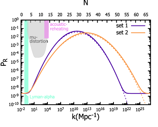
Figure 4: The power specta in the slow-roll approximation (solid lines) and using the exact equation (3.27) of perturbations (dashed lines). Purple line corresponds to the set 1 and orange line to set 2, given in Table 1. Details are on main text.

In Fig. 4 we present the exact (numerical) and analytical (in the slow-roll approximation) power spectrum for the potential (2.16). In this plot we also depict for comparison reasons the current bounds from the Lyman-alpha forest [90], the mu-distortion [91] and the acoustic-reheating bound [92, 93]. The exact results are plotted as dashed lines and the slow-roll analytical results as solid lines. For the analytical expression we use the Eq. (3.23) and for the numerical expression we use the Eq. (3.27). For the numerical evaluation we follow the analysis described in Refs. [70, 86]. Specifically, we solve numerically the background equations (3.2), the fields’ perturbation (3.25) and the Bardeen potential (3.26) simultaneously until the end of inflation (the parameter $\varepsilon$ reaches value 1) starting from the critical point as initial condition. We obtain at around 27 efold, as it is shown in Fig.3. We integrate again the system of the different equations, (3.2), 3.25) and (3.26), until $k=0.05Mpc^{-1}$ and we find the initial conditions and we obtain the rest number of efold. Finally, we integrate again the system from the new initial conditions until the end of inflation. We notice that the analytical and the numerical results are very similar, as it is expected [70]. Therefore for convenience we shall use the analytical slow-roll solution hereinafter.

4 Gravitational Waves Production

In the previous sections, we have presented a mechanism in the context of a SUGRA based hybrid model, that can produce a significant enhancement in the scalar power spectrum. The amount of GWs is evaluated by the second-order (tensor) perturbations, which appear as $h_{ij}$ in Eq. (3.24). However, the tensor second-order perturbations can be related to the scalar first-order perturbations, and hence to the scalar power spectrum [94, 95, 96, 97, 98, 99, 100]. In this section we show that the enhancement of the power spectrum can be interpreted as a source of GWs created during the radiation dominance era.

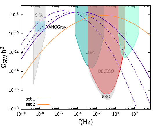
Figure 5: The energy density of gravitational waves for the analytical expression Eq. (3.23). Purple curves correspond to set 1 and the orange to set 2, as given in Table 1. Detailed description of the various curve shapes can be found in the main text.

The present-day energy density of the GWs is [101]

$${\Omega_{GW}(k)}=\frac{1}{24}\left(\frac{k}{aH}\right)^{2}\overline{P_{h}(\tau,k)}\,,$$ (4.1)

where $P_{h}$ is the tensor perturbation and the over-line denotes the average over the time. In terms of scalar power spectrum this expression reads as [98]:

$${\Omega_{GW}(k)}=\frac{c_{g}\,\Omega_{r}}{36}\int^{\frac{1}{\sqrt{3}}}_{0}\mathrm{d}d\int^{\infty}_{\frac{1}{\sqrt{3}}}\mathrm{d}s\left[\frac{(s^{2}-1/3)(d^{2}-1/3)}{s^{2}+d^{2}}\right]^{2}\,P_{R}(kx)P_{R}(ky)(I_{c}^{2}+I_{s}^{2}).$$ (4.2)

The radiation density $\Omega_{r}$ gets its measured present day value $\Omega_{r}=5.4\times 10^{-5}$ and $c_{g}=0.4$ in the case of Standard Model (SM) spectrum, while $c_{g}=0.3$ in the Minimal Supersymmetric SM (MSSM). The variables $x$ and $y$ are:

$$x=\frac{\sqrt{3}}{2}(s+d),\quad y=\frac{\sqrt{3}}{2}(s-d).$$ (4.3)

Finally, the functions $I_{c}$ and $I_{s}$ are given by the equations

$$I_{c}=-36\,\pi\,\frac{(s^{2}+d^{2}-2)^{2}}{(s^{2}-d^{2})^{3}}\,\Theta(s-1)$$ (4.4)

$$I_{s}=-36\,\frac{(s^{2}+d^{2}-2)^{2}}{(s^{2}-d^{2})^{2}}\Bigg{[}\frac{(s^{2}+d^{2}-2)}{(s^{2}-d^{2})}\,\ln\left|\frac{d^{2}-1}{s^{2}-1}\right|+2\Bigg{]}\,.$$ (4.5)

Using that $1\,\mathrm{Mpc}^{-1}=0.97154\times 10^{-14}\,\mathrm{s}^{-1}$ and $k=2\pi f$, we can evaluate the energy density of the GWs as a function of the frequency.

In Fig. 5 we plot the energy density of GWs using the analytical expression in Eq. (3.23). Purple curves correspond to set 1 and the orange to set 2, as given in Table 1. Moreover, the solid (dashed, dashed-double dot) purple line correspond to $a_{1}=4.33$ ($a_{1}=5$, $a_{1}=6$), in units $10^{-7}/M_{P}$. The parameter $a_{1}$ is defined in (2.17). As can be seen from the figure, the predicted GW spectra for these parameter choices, in the context of our hybrid model, lie well within the detection range of the future GW experiments, like LISA, DESIGO, BBO, SKA and ET [7, 8, 9, 12, 10]. Interestingly enough, we notice that the recently reported NANOGrav [5, 6, 4] signal of can be interpreted in the context of this model (purple lines). In this figure we display the NANOGrav 12.5 yrs region.

5 Primordial Black Holes Abundance

The significant enhancement of scalar power spectrum not only can explain the energy density of GWs, as it is was discussed in the previous section, but also the production of the PBHs. A main result of Ref. [102] is that the GWs spectrum , which is compatible to the NANOGrav region, can be related to a particular prediction for the PBH abundance. In this section we evaluate the mass of PBHs and their fractional abundances. As usual it is assumed that the PBH are formed in the radiation dominated epoch, as the GWs.

The fractional abundance of PBHs, $\Omega_{PBH}/\Omega_{DM}$, can be evaluated as a function of the PBH mass using that

$$\frac{\Omega_{PBH}}{\Omega_{DM}}(M_{\mathrm{PBH}})=\frac{\beta(M_{\mathrm{PBH}})}{8\times 10^{-16}}\left(\frac{\gamma}{0.2}\right)^{3/2}\left(\frac{g_{*}(T_{f})}{106.75}\right)^{-1/4}\left(\frac{M_{\mathrm{PBH}}\,}{10^{-18}\;\mathrm{grams}}\right)^{-1/2}\,,$$ (5.1)

where we assume that the DM abundance is $\Omega_{DM}\simeq 0.26$. With $\gamma$ we denote a factor which depends on the gravitation collapse and we choose $\gamma=0.2$ [103]. With $\beta$ we denote the mass fraction of Universe collapsing in PBH mass. The $T_{f}$ denotes the temperature of PBH formation and the $g_{*}(T_{f})$ are the effective degrees of freedom during this formation. In order to evaluate the abundance of PBHs, we integrate the expression in Eq. (5.1) as

$$f_{PBH}=\int\frac{dM_{\mathrm{PBH}}}{M_{\mathrm{PBH}}}\,\frac{\Omega_{PBH}}{\Omega_{DM}}\,.$$ (5.2)

The mass of PBHs, which are created after the inflation when the scales reenter the horizon is related to the mass inside the Hubble horizon. Specifically, the mass of PBHs is

$$M_{\mathrm{PBH}}=\gamma\frac{4\,\pi\,\rho}{3}H^{-3}\,,$$ (5.3)

where $\rho$ is the energy density of Universe during collapse. If we consider that the PBHs are formed during the radiation epoch, their mass is [13]

$$M_{\mathrm{PBH}}=\gamma\frac{4\,\pi\,\rho}{3}\,H_{m-r}^{-3}\left(\frac{g(T_{f})}{g(T_{m-r})}\right)^{1/2}\left(\frac{g_{s}(T_{f})}{g_{s}(T_{m-r})}\right)^{-2/3}\left(\frac{k}{k_{m-r}}\right)^{-2}\,,$$ (5.4)

where the subscript ${m-r}$ refers to the time of equality of matter and radiation domination and $g_{s}$ refers to the entropy density. The equation above arises from the entropy conservation $d(g_{s}(T)T^{3}a^{3})/dt=0$ between the epoch of the reentry of the comoving wavenumbers and the epoch of radiation-matter equality. Thus we can express the mass of PBHs as a function of the comoving wavenumber $k$

$$M_{\mathrm{PBH}}(k)=10^{18}\left(\frac{\gamma}{0.2}\right)\left(\frac{g_{*}(T_{f})}{106.75}\right)^{-1/6}\left(\frac{k}{7\times 10^{13}\,\mathrm{Mpc}^{-1}}\right)^{-2}\mathrm{in\leavevmode\nobreak\ grams}\,,$$ (5.5)

where we use the approximation $g(T)=g_{s}(T)$ [13]. Assuming that the spectrum of the our model is like the SM, we can use ${g_{*}(T)=106.75}$. On the other hand assuming a spectrum like the MSSM, we get $g_{*}(T)=228.75$. Thus the PBH fractional abundance in the SM is 1.13 times larger than in the MSSM. This relative factor to a good approximation can be ignored.

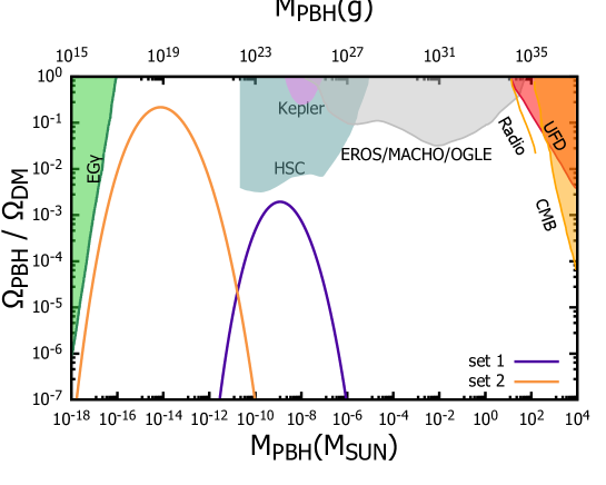
Figure 6: The fractional abundance of PBHs as a function of mass. As before, the purple line corresponds to set 1 and orange line to set 2 given in Table 1.

The mass fraction $\beta$ is evaluated using the Press-Schechter approach. In this approach, the mass fraction $\beta$ is calculated assuming that the overdensity $\delta$ follows a gaussian probability, with a threshold of collapse $\delta_{c}$. So the mass fraction is given from the integral

$$\beta(M_{\mathrm{PBH}})=\frac{1}{\sqrt{2\pi\sigma^{2}(M_{\mathrm{PBH}})}}\int^{\infty}_{\delta_{c}}d\delta\,\exp\left(-\frac{\delta^{2}}{2\sigma^{2}(M_{\mathrm{PBH}})}\right)\,,$$ (5.6)

where $\sigma$ is the variance of curvature perturbation, related to the comoving wavenumber as

$$\sigma^{2}\left(M_{\mathrm{PBH}}(k)\right)=\frac{16}{81}\int\frac{dk^{\prime}}{k^{\prime}}\left(\frac{k^{\prime}}{k}\right)^{4}P_{R}(k^{\prime})\tilde{W}\left(\frac{k^{\prime}}{k}\right).$$ (5.7)

where $\tilde{W}(x)$ is a window function. We consider the Gaussian distribution for this function: $\tilde{W}(x)=e^{-x^{2}/2}$. For $\delta_{c}$, following recent studies [104, 105, 106, 107, 108, 109, 110, 111], we consider values in the range between 0.4 and 0.6.

In Fig. 6 we plot the fractional abundance of PBHs from Eq. (5.1). We use the analytical expression for the scalar power spectrum from Eq. (3.23). In this plot we use the value of the $\delta_{c}=0.50$ for the set 1 (purple curve) and $\delta_{c}=0.43$ for the set 2 (orange curve). In both cases, a significant fractional abundance of PBHs is obtained. To form an idea of the allowed parameter space, in the Fig. 6 we also display the disallowed regions due to various observational groups and studies [112, 113, 114, 115, 116, 117, 118, 119, 120, 121, 122, 123].

Specifically, we notice a tension between the NANOGrav data for the GW spectrum and the SUBARU HSC experiment exclusion limit for the PBH fraction. As a result of this, for the set 1 (purple curve) the calculated abundance of PBHs from Eq. (5.2) is ${f_{PBH}\simeq 0.01}$, while for set 2 (orange line) we get $f_{PBH}\simeq 1$. That is, in former case PBH can account just for the ${1\%}$ of the DM of the Universe, while in the latter can be almost $100\%$. In order to understand this one has to compare Fig. 6 with Fig. 5. In particular, in Fig. 5 the frequency $f$ is proportional to comoving wavenumber $k$, but the $M_{\mathrm{PBH}}$ in Fig. 6 is proportional to $k^{-2}$. Thus, to fulfil the NANOGrav region result to move the GW spectrum to the right close to the disallowed regions. In any case, the hybrid model under consideration can be regarded as proper candidate to explain the whole DM in the Universe. Finally, hybrid models can also explain the production of PBHs in a wide range of masses.

6 Fine-tuning estimation and Conclusions

A drawback of the models, where an enhancement of scalar power spectrum is produced due to a modification of the potential, is the high level of required fine-tuning of the parameters involved in this modification. In particular, models, where an inflection point in effective scalar potential is developed, demand a significant amount of fine -tuning [20, 21]. In this section we perform an analogous study for the hybrid model under consideration and we show that the corresponding amount of the fine-tuning is much smaller, at least by 3 or 4 orders of magnitudes.

As discussed in Section 2, the basis of our hybrid model is the original hybrid model introduced in [43], with the addition of extra SUGRA terms, that correct the value of the spectral index $n_{s}$. Hence, we have had two extra parameters, $b_{1}$ and $b_{2}$. Generally speaking, using the parameter $b_{2}$ we decreased the value of the $n_{s}$ to be in accordance with the observable constraints, while the other parameter $b_{1}$ is used for explaining the enhancement in power spectrum and then the production of GWs and PBHs.

In order to have a measure of the required fine-tuning in this model, we calculate the quantity $\Delta_{p}$, as discussed in [124], for the parameter $b_{1}$. $\Delta_{p}$ is the maximum value of the logarithmic derivative of the peak value of the power spectrum, with respect to $b_{1}$

$$\Delta_{p}=\mathrm{Max}\left|\frac{\partial\ln(P_{R}^{PEAK})}{\partial\ln(b_{1})}\right|.$$ (6.1)

The larger the $\Delta_{p}$, the larger the amount of the required fine-tuning. Evaluating numerically $\Delta_{p}$ from Eq. (6.1), for the function $P_{R}^{(peak)}(b_{1})$ we find that $\Delta_{p}\sim 100$, if we demand a peak of power spectrum at around $5\times 10^{-2}$. Thus, we conclude that the amount of the fine -tuning is significantly smaller, by almost four orders of magnitude in the case of this hybrid model, compared to the single field inflation models, where an inflection point is the source for producing PBHs [20]. Finally, we notice here that the fine-tuning for an acceptable values for the $n_{s}$ is mainly based on the parameter $b_{2}$ and this issue. For analogous equation of Eq. (6.1) we obtain a quantity at $\Delta_{p}\sim 10$ in the range near to $b_{2}$.

Concluding, in this work we presented a two-field inflationary model based on the original simple hybrid model, in order to explain the generation of both GWs and PBHs. The effective scalar potentials derived by hybrid models have the advantage that they do not require a high level of fine-tuning of the parameters in order to describe an amplification in scalar power spectrum. As the issue of fine-tuning is regarded as a main problematic feature in many proposed models, studying hybrid models should be a plausible scenario in order to describe enhancement in scalar power spectrum. A disadvantage of these models is that they cannot predict acceptable values for the spectral index $n_{s}$. For this reason we introduced specific SUGRA-type corrections in the inflaton field, where we evaluated the prediction for the cosmological constraints. In our proposed model we have achieved acceptable values for both spectral index and tensor-to-scalar ratio.

Hybrid models can explain the production of GWs and PBHs due to the amplification of the scalar power spectrum. This enhancement occurs because of the mild waterfall of one of the two fields. We presented an analytical procedure for evaluating the scalar power spectrum of our proposed model based on slow-roll approximation. For comparison, we evaluated numerically the exact equations of perturbations by using the exact proposed potential. We conclude that the results for analytical and numerical procedure are quite similar, since they differ up to $10\%$.

Having calculated the scalar power spectrum we evaluated the amount of the produced GWs in the radiation dominated epoch. To facilitate the phenomenological analysis of our model we have chose two representative sets of the two parameters for the extra terms in the Kähler potential. The first set corresponds to a model that predicts GW spectra that lie within the NANOGrav detection region. Unfortunately the associated factional abundance of PBHs is restricted by the SUBARU HSC exclusion region. As a result in this case only 1% of DM can be interpreted by PBHs. On the other hand, in the second set we relax the NANOGrav constrain. This way we are able to increase the factional abundance of PBHs up to 100%.

Appendix A Appendix

In order to evaluate the SUGRA corrections in the scalar potential, we consider the Kähler potential:

$${K=S\bar{S}+b_{1}(S+\bar{S})+b_{2}(S+\bar{S})^{2}+\Psi_{1}{\bar{\Psi}_{1}}+\Psi_{2}{\bar{\Psi}_{2}}}\,$$ (A.1)

and we assume that the superpotential is given from

$$W=\kappa\,S(\Psi_{1}{\Psi}_{2}-\frac{M^{2}}{2})\,$$ (A.2)

We calculate the $F$-term of scalar potential from Eq. (2.11) and we find

$${\begin{split}V_{F}^{\text{SUGRA}}&={\frac{\kappa^{2}}{4{M_{P}}^{4}}}\exp[\frac{1}{M_{P}^{2}}\left(\frac{b_{1}\phi}{\sqrt{b_{2}+\frac{1}{2}}}+\frac{{b_{2}}\phi^{2}}{b_{2}+\frac{1}{2}}+\frac{\phi^{2}}{4b_{2}+2}+{\psi^{2}}\right)\Bigg{]}\\ &\times\Bigg{[}\frac{\left(M^{2}-\psi^{2}\right)^{2}\left({b_{1}}\sqrt{4{b_{2}}+2}\phi+(4{b_{2}}+2){M_{P}}^{2}+(4{b_{2}}+1)\phi^{2}\right)^{2}}{4(2{b_{2}}+1)^{3}}\\ &+\frac{\phi^{2}\psi^{2}\left(-M^{2}+2{M_{P}}^{2}+\psi^{2}\right)^{2}}{4{b_{2}}+2}-\frac{3{M_{P}}^{2}\phi^{2}\left(M^{2}-\psi^{2}\right)^{2}}{4b_{2}+2}\Bigg{]}\end{split}}$$ (A.3)

where we have fix the non-canonical kinetic terms by the definition of the chiral fields

$$S=\frac{\phi}{\sqrt{2+4b_{2}}},\quad|\Psi_{1}|=|{\Psi}_{2}|={\psi/\sqrt{2}}.$$ (A.4)

Moreover, we derive the scalar potential using the general form

$$\begin{split}V_{F}^{\text{SUGRA}}&=\left(1+\frac{K}{M_{P}^{2}}+\frac{K^{2}}{2M_{P}^{4}}+\frac{K^{3}}{6M_{P}^{6}}\right)\\ &\times\left[\left({K^{-1}}\right)^{i}_{\bar{j}}\left(W^{\bar{j}}+\frac{WK^{\bar{j}}}{{M_{P}}^{2}}\right)\left(\bar{W}_{i}+\frac{\bar{W}K_{i}}{{M_{P}}^{2}}\right)-\frac{3|W|^{2}}{{M_{P}}^{2}}\right]\end{split}$$ (A.5)

and we have

$$V_{F}^{\text{SUGRA}}=\frac{\kappa^{2}(M^{4}-2M^{2}\psi^{2}+2\psi^{2}\phi^{2}+\psi^{4})}{4+8b_{2}}+\frac{\mathcal{A}_{1}}{M_{P}^{2}}+\frac{\mathcal{A}_{2}}{M_{P}^{4}}+\frac{\mathcal{A}_{3}}{M_{P}^{6}}+\mathcal{O}\left(\frac{1}{M_{P}^{8}}\right)$$ (A.6)

In the limit $M_{P}\rightarrow\infty$ we derive the SUSY scalar potential. The SUGRA corrections $\mathcal{A}_{1}$, $\mathcal{A}_{2}$ and $\mathcal{A}_{3}$ are calculated as

$$\begin{split}\mathcal{A}_{1}=&\frac{\kappa^{2}}{4(2b_{2}+1)^{5/2}}\Big{[}2\sqrt{2}{b_{1}}(2{b_{2}}+1)\phi\left(M^{4}-2m^{2}\psi^{2}+\phi^{2}\psi^{2}+\psi^{4}\right)+\\ +&2\sqrt{2}{b_{1}}(2{b_{2}}+1)\phi\left(M^{4}-2M^{2}\psi^{2}+\phi^{2}\psi^{2}+\psi^{4}\right)+\\ +&{b_{2}}\Big{(}M^{4}\left(3\phi^{2}+2\psi^{2}\right)+2M^{2}\psi^{2}\left(-5\phi^{2}-2\psi^{2}+2M_{P}^{2}\right)+\\ +&\psi^{2}\left(4\phi^{4}+11\phi^{2}\psi^{2}-2M_{P}^{2}\left(2\phi^{2}+3\psi^{2}\right)+2\psi^{4}\right)\Big{)}\Big{]}\end{split}$$ (A.7)

$$\begin{split}\mathcal{A}_{2}=&\frac{\kappa^{2}}{32(2{b_{2}}+1)^{7/2}}\Big{[}4{b_{1}}^{2}(2{b_{2}}+1)^{3/2}\phi^{2}\left(7M^{4}-14M^{2}\psi^{2}+4\phi^{2}\psi^{2}+7\psi^{4}\right)+\\ +&8\sqrt{2}{b_{1}}\phi\Big{(}\left(8{b_{2}}^{2}+6{b_{2}}+1\right)\phi^{4}\psi^{2}+5\left(6{b_{2}}^{2}+5{b_{2}}+1\right)\phi^{2}\psi^{4}+\\ +&(2{b_{2}}+1)M^{4}\left((7{b_{2}}+1)\phi^{2}+2(2{b_{2}}+1)\psi^{2}\right)-\\ -&2(2{b_{2}}+1)M^{2}\psi^{2}\left((9{b_{2}}+2)\phi^{2}+2(2{b_{2}}+1)\psi^{2}\right)+2(2{b_{2}}+1)^{2}\psi^{6}\Big{)}+\\ +&\sqrt{2{b_{2}}+1}\Big{(}M^{4}\big{[}\left(64{b_{2}}^{2}+20{b_{2}}+1\right)\phi^{4}+\\ +&4\left(16{b_{2}}^{2}+10{b_{2}}+1\right)\phi^{2}\psi^{2}+4(2{b_{2}}+1)^{2}\psi^{4}\big{]}-\\ -&2M^{2}\psi^{2}\big{[}\left(96{b_{2}}^{2}+44{b_{2}}+5\right)\phi^{4}+12\left(8{b_{2}}^{2}+6{b_{2}}+1\right)\phi^{2}\psi^{2}-\\ -&8(2{b_{2}}+1)^{2}{M_{P}}^{4}+4(2{b_{2}}+1)^{2}\psi^{4}\big{]}+\\ +&\psi^{2}\big{[}\left(192{b_{2}}^{2}+116{b_{2}}+17\right)\phi^{4}\psi^{2}+4\left(40{b_{2}}^{2}+34{b_{2}}+7\right)\phi^{2}\psi^{4}-\\ -&8(2{b_{2}}+1)^{2}{M_{P}}^{4}\left(2\phi^{2}+3\psi^{2}\right)+2(4{b_{2}}+1)^{2}\phi^{6}+4(2{b_{2}}+1)^{2}\psi^{6}\big{]}\Big{)}\Big{]}\end{split}$$ (A.8)

$$\begin{split}\mathcal{A}_{3}=&\frac{\kappa^{2}}{96(2{b_{2}}+1)^{9/2}}\Big{[}4\sqrt{2}{b_{1}}^{3}(2{b_{2}}+1)^{2}\phi^{3}\left(11M^{4}-22M^{2}\psi^{2}+4\phi^{2}\psi^{2}+11\psi^{4}\right)+\\ +&6{b_{1}}^{2}\sqrt{2{b_{2}}+1}\phi^{2}\Big{(}4\left(8{b_{2}}^{2}+6{b_{2}}+1\right)\phi^{4}\psi^{2}+5\left(32{b_{2}}^{2}+26{b_{2}}+5\right)\phi^{2}\psi^{4}+\\ +&(2{b_{2}}+1)M^{4}\left((48{b_{2}}+9)\phi^{2}+14(2{b_{2}}+1)\psi^{2}\right)-\\ -&2(2{b_{2}}+1)M^{2}\psi^{2}\big{[}(56{b_{2}}+13)\phi^{2}+14(2{b_{2}}+1)\psi^{2}\big{)}+14(2{b_{2}}+1)^{2}\psi^{6}\Big{)}+\\ +&6\sqrt{2}{b_{1}}\phi\Big{(}2M^{4}\big{(}\left(56{b_{2}}^{3}+50{b_{2}}^{2}+13{b_{2}}+1\right)\phi^{4}+\\ +&(16{b_{2}}+3)\phi^{2}(2{b_{2}}\psi+\psi)^{2}+2(2{b_{2}}+1)^{3}\psi^{4}\big{]}-\\ -&4M^{2}\psi^{2}\left(\left(72{b_{2}}^{3}+70{b_{2}}^{2}+21{b_{2}}+2\right)\phi^{4}+5(4{b_{2}}+1)\phi^{2}(2{b_{2}}\psi+\psi)^{2}+2(2{b_{2}}+1)^{3}\psi^{4}\right)+\\ +&10\left(24{b_{2}}^{3}+26{b_{2}}^{2}+9{b_{2}}+1\right)\phi^{4}\psi^{4}+(2{b_{2}}+1)\phi^{6}(4{b_{2}}\psi+\psi)^{2}+\\ +&2(28{b_{2}}+9)\psi^{6}(2{b_{2}}\phi+\phi)^{2}+4(2{b_{2}}+1)^{3}\psi^{8}\Big{)}+\\ +&\sqrt{2{b_{2}}+1}\Big{(}M^{4}\big{[}3\left(160{b_{2}}^{3}+144{b_{2}}^{2}+38{b_{2}}+3\right)\phi^{4}\psi^{2}+(4{b_{2}}+1)^{2}(17{b_{2}}+2)\phi^{6}+\\ +&12(5{b_{2}}+1)\psi^{4}(2{b_{2}}\phi+\phi)^{2}+4(2{b_{2}}+1)^{3}\psi^{6}\big{]}+\\ +&\psi^{2}\big{[}3\left(352{b_{2}}^{3}+384{b_{2}}^{2}+134{b_{2}}+15\right)\phi^{4}\psi^{4}-\\ -&24(2{b_{2}}+1)^{3}{M_{P}}^{6}\left(2\phi^{2}+3\psi^{2}\right)+(4{b_{2}}+1)^{3}\phi^{8}+\\ +&(41{b_{2}}+14)\phi^{6}(4b_{2}\psi+\psi)^{2}+4(31{b_{2}}+11)\psi^{6}(2{b_{2}}\phi+\phi)^{2}+4(2b_{2}+1)^{3}\psi^{8}\big{]}-\\ -&2M^{2}\psi^{2}\big{[}-24(2{b_{2}}+1)^{3}{M_{P}}^{6}+(4{b_{2}}+1)^{2}(23b_{2}+5)\phi^{6}+\\ +&21(2b_{2}+1)\phi^{4}(4b_{2}\psi+\psi)^{2}+12(7b_{2}+2)\psi^{4}(2{b_{2}}\phi+\phi)^{2}+4(2b_{2}+1)^{3}\psi^{6}\big{]}\Big{)}\Big{]}\end{split}$$ (A.9)

we derive that around the critical point $\phi_{c}=0.05M_{P}$ the numerical values of the corrections are: $\mathcal{A}_{1}/{{M_{P}}^{6}\kappa^{2}}\approx 10^{-9}$, $\mathcal{A}_{2}/{{M_{P}}^{8}\kappa^{2}}\approx 10^{-10}$ and $\mathcal{A}_{3}/{{M_{P}}^{12}\kappa^{2}}\approx 10^{-12}$. Moreover for these parameters, the spectral index is $n_{s}={0.96505}$. If we consider corrections up to $\mathcal{O}(1/{M_{p}}^{2})$ we derive $n_{s}={0.9577}$. Therefore, it is essential for the precise $n_{s}$ calculation to include corrections up to $\mathcal{O}(1/{M_{p}}^{4})$.

References

- [1] B. Abbott et al. [LIGO Scientific and Virgo], Phys. Rev. Lett. 116 (2016) no.6, 061102 doi:10.1103/PhysRevLett.116.061102 [arXiv:1602.03837 [gr-qc]].
- [2] B. P. Abbott et al. [LIGO Scientific and Virgo], Phys. Rev. Lett. 116 (2016) no.24, 241103 doi:10.1103/PhysRevLett.116.241103 [arXiv:1606.04855 [gr-qc]].
- [3] B. Abbott et al. [LIGO Scientific and Virgo], Phys. Rev. Lett. 119 (2017) no.14, 141101 doi:10.1103/PhysRevLett.119.141101 [arXiv:1709.09660 [gr-qc]].
- [4] Z. Arzoumanian et al. [NANOGrav], Astrophys. J. Lett. 905 (2020) no.2, L34 doi:10.3847/2041-8213/abd401 [arXiv:2009.04496 [astro-ph.HE]].
- [5] Z. Arzoumanian et al. [NANOGRAV], Astrophys. J. 859 (2018) no.1, 47 doi:10.3847/1538-4357/aabd3b [arXiv:1801.02617 [astro-ph.HE]].
- [6] K. Aggarwal, Z. Arzoumanian, P. T. Baker, A. Brazier, M. R. Brinson, P. R. Brook, S. Burke-Spolaor, S. Chatterjee, J. M. Cordes and N. J. Cornish, et al. Astrophys. J. 880 (2019), 2 doi:10.3847/1538-4357/ab2236 [arXiv:1812.11585 [astro-ph.GA]].
- [7] P. Amaro-Seoane et al. [LISA], [arXiv:1702.00786 [astro-ph.IM]].
- [8] S. Sato, S. Kawamura, M. Ando, T. Nakamura, K. Tsubono, A. Araya, I. Funaki, K. Ioka, N. Kanda and S. Moriwaki, et al. J. Phys. Conf. Ser. 840 (2017) no.1, 012010 doi:10.1088/1742-6596/840/1/012010
- [9] B. S. Sathyaprakash and B. F. Schutz, Living Rev. Rel. 12 (2009), 2 doi:10.12942/lrr-2009-2 [arXiv:0903.0338 [gr-qc]].
- [10] K. Yagi and N. Seto, Phys. Rev. D 83 (2011), 044011 [erratum: Phys. Rev. D 95 (2017) no.10, 109901] doi:10.1103/PhysRevD.83.044011 [arXiv:1101.3940 [astro-ph.CO]].
- [11] J. Luo et al. [TianQin], Class. Quant. Grav. 33 (2016) no.3, 035010 doi:10.1088/0264-9381/33/3/035010 [arXiv:1512.02076 [astro-ph.IM]].
- [12] W. Zhao, Y. Zhang, X. P. You and Z. H. Zhu, Phys. Rev. D 87 (2013) no.12, 124012 doi:10.1103/PhysRevD.87.124012 [arXiv:1303.6718 [astro-ph.CO]].
- [13] G. Ballesteros and M. Taoso, Phys. Rev. D 97 (2018) no.2, 023501 doi:10.1103/PhysRevD.97.023501 [arXiv:1709.05565 [hep-ph]].
- [14] T. Gao and Z. Guo, Phys. Rev. D 98 (2018) no.6, 063526 doi:10.1103/PhysRevD.98.063526 [arXiv:1806.09320 [hep-ph]].
- [15] M. Cicoli, V. A. Diaz and F. G. Pedro, JCAP 06 (2018), 034 doi:10.1088/1475-7516/2018/06/034 [arXiv:1803.02837 [hep-th]].
- [16] I. Dalianis, A. Kehagias and G. Tringas, JCAP 01 (2019), 037 doi:10.1088/1475-7516/2019/01/037 [arXiv:1805.09483 [astro-ph.CO]].
- [17] J. Garcia-Bellido and E. Ruiz Morales, Phys. Dark Univ. 18 (2017), 47-54 doi:10.1016/j.dark.2017.09.007 [arXiv:1702.03901 [astro-ph.CO]].
- [18] J. M. Ezquiaga, J. Garcia-Bellido and E. Ruiz Morales, Phys. Lett. B 776 (2018), 345-349 doi:10.1016/j.physletb.2017.11.039 [arXiv:1705.04861 [astro-ph.CO]].
- [19] D. V. Nanopoulos, V. C. Spanos and I. D. Stamou, Phys. Rev. D 102 (2020) no.8, 083536 doi:10.1103/PhysRevD.102.083536 [arXiv:2008.01457 [astro-ph.CO]].
- [20] I. D. Stamou, Phys. Rev. D 103 (2021) no.8, 083512 doi:10.1103/PhysRevD.103.083512 [arXiv:2104.08654 [hep-ph]].
- [21] M. P. Hertzberg and M. Yamada, Phys. Rev. D 97 (2018) no.8, 083509 doi:10.1103/PhysRevD.97.083509 [arXiv:1712.09750 [astro-ph.CO]].
- [22] G. Ballesteros, J. Rey and F. Rompineve, JCAP 06 (2020), 014 doi:10.1088/1475-7516/2020/06/014 [arXiv:1912.01638 [astro-ph.CO]].
- [23] K. Kefala, G. P. Kodaxis, I. D. Stamou and N. Tetradis, [arXiv:2010.12483 [astro-ph.CO]].
- [24] I. Dalianis, G. P. Kodaxis, I. D. Stamou, N. Tetradis and A. Tsigkas-Kouvelis, [arXiv:2106.02467 [astro-ph.CO]].
- [25] M. Braglia, D. K. Hazra, L. Sriramkumar and F. Finelli, JCAP 08 (2020), 025 doi:10.1088/1475-7516/2020/08/025 [arXiv:2004.00672 [astro-ph.CO]].
- [26] M. Braglia, D. K. Hazra, F. Finelli, G. F. Smoot, L. Sriramkumar and A. A. Starobinsky, JCAP 08 (2020), 001 doi:10.1088/1475-7516/2020/08/001 [arXiv:2005.02895 [astro-ph.CO]].
- [27] M. Braglia, X. Chen and D. K. Hazra, JCAP 03 (2021), 005 doi:10.1088/1475-7516/2021/03/005 [arXiv:2012.05821 [astro-ph.CO]].
- [28] G. A. Palma, S. Sypsas and C. Zenteno, Phys. Rev. Lett. 125 (2020) no.12, 121301 doi:10.1103/PhysRevLett.125.121301 [arXiv:2004.06106 [astro-ph.CO]].
- [29] J. Fumagalli, S. Renaux-Petel, J. W. Ronayne and L. T. Witkowski, [arXiv:2004.08369 [hep-th]].
- [30] A. Gundhi, S. V. Ketov and C. F. Steinwachs, Phys. Rev. D 103 (2021) no.8, 083518 doi:10.1103/PhysRevD.103.083518 [arXiv:2011.05999 [hep-th]].
- [31] M. Khlopov, Symmetry 7 (2015) no.2, 815-842 doi:10.3390/sym7020815 [arXiv:1505.08077 [astro-ph.CO]].
- [32] S. V. Ketov and M. Y. Khlopov, Symmetry 11 (2019) no.4, 511 doi:10.3390/sym11040511
- [33] S. Mukherjee and J. Silk, doi:10.1093/mnras/stab1932 [arXiv:2105.11139 [gr-qc]].
- [34] S. Mukherjee, M. S. P. Meinema and J. Silk, [arXiv:2107.02181 [astro-ph.CO]].
- [35] S. Vagnozzi, Mon. Not. Roy. Astron. Soc. 502 (2021) no.1, L11-L15 doi:10.1093/mnrasl/slaa203 [arXiv:2009.13432 [astro-ph.CO]].
- [36] S. Pi, Y. l. Zhang, Q. G. Huang and M. Sasaki, JCAP 05 (2018), 042 doi:10.1088/1475-7516/2018/05/042 [arXiv:1712.09896 [astro-ph.CO]].
- [37] R. G. Cai, Z. K. Guo, J. Liu, L. Liu and X. Y. Yang, JCAP 06 (2020), 013 doi:10.1088/1475-7516/2020/06/013 [arXiv:1912.10437 [astro-ph.CO]].
- [38] K. Kohri and T. Terada, Phys. Lett. B 813 (2021), 136040 doi:10.1016/j.physletb.2020.136040 [arXiv:2009.11853 [astro-ph.CO]].
- [39] A. Ashoorioon, A. Rostami and J. T. Firouzjaee, JHEP 07 (2021), 087 doi:10.1007/JHEP07(2021)087 [arXiv:1912.13326 [astro-ph.CO]].
- [40] A. Ashoorioon, A. Rostami and J. T. Firouzjaee, Phys. Rev. D 103 (2021), 123512 doi:10.1103/PhysRevD.103.123512 [arXiv:2012.02817 [astro-ph.CO]].
- [41] J. A. Adams, B. Cresswell and R. Easther, Phys. Rev. D 64 (2001), 123514 doi:10.1103/PhysRevD.64.123514 [arXiv:astro-ph/0102236 [astro-ph]].
- [42] D. K. Hazra, M. Aich, R. K. Jain, L. Sriramkumar and T. Souradeep, JCAP 10 (2010), 008 doi:10.1088/1475-7516/2010/10/008 [arXiv:1005.2175 [astro-ph.CO]].
- [43] A. D. Linde, Phys. Rev. D 49 (1994), 748-754 doi:10.1103/PhysRevD.49.748 [arXiv:astro-ph/9307002 [astro-ph]].
- [44] A. D. Linde, Phys. Lett. B 259 (1991), 38-47 doi:10.1016/0370-2693(91)90130-I
- [45] E. J. Copeland, A. R. Liddle, D. H. Lyth, E. D. Stewart and D. Wands, Phys. Rev. D 49 (1994), 6410-6433 doi:10.1103/PhysRevD.49.6410 [arXiv:astro-ph/9401011 [astro-ph]].
- [46] S. Mollerach, S. Matarrese and F. Lucchin, Phys. Rev. D 50 (1994), 4835-4841 doi:10.1103/PhysRevD.50.4835 [arXiv:astro-ph/9309054 [astro-ph]].
- [47] A. D. Linde and A. Riotto, Phys. Rev. D 56 (1997), R1841-R1844 doi:10.1103/PhysRevD.56.R1841 [arXiv:hep-ph/9703209 [hep-ph]].
- [48] Y. Akrami et al. [Planck], Astron. Astrophys. 641 (2020), A10 doi:10.1051/0004-6361/201833887 [arXiv:1807.06211 [astro-ph.CO]].
- [49] P. Ade et al. [Planck], Astron. Astrophys. 594 (2016), A20 doi:10.1051/0004-6361/201525898 [arXiv:1502.02114 [astro-ph.CO]].
- [50] G. R. Dvali, Q. Shafi and R. K. Schaefer, Phys. Rev. Lett. 73 (1994), 1886-1889 doi:10.1103/PhysRevLett.73.1886 [arXiv:hep-ph/9406319 [hep-ph]].
- [51] M. Bastero-Gil, S. F. King and Q. Shafi, Phys. Lett. B 651 (2007), 345-351 doi:10.1016/j.physletb.2006.06.085 [arXiv:hep-ph/0604198 [hep-ph]].
- [52] S. Dimopoulos, G. R. Dvali and R. Rattazzi, Phys. Lett. B 410 (1997), 119-124 doi:10.1016/S0370-2693(97)00970-2 [arXiv:hep-ph/9705348 [hep-ph]].
- [53] G. R. Dvali, G. Lazarides and Q. Shafi, Phys. Lett. B 424 (1998), 259-264 doi:10.1016/S0370-2693(98)00145-2 [arXiv:hep-ph/9710314 [hep-ph]].
- [54] C. Panagiotakopoulos and N. Tetradis, Phys. Rev. D 59 (1999), 083502 doi:10.1103/PhysRevD.59.083502 [arXiv:hep-ph/9710526 [hep-ph]].
- [55] N. Tetradis, Phys. Rev. D 57 (1998), 5997-6002 doi:10.1103/PhysRevD.57.5997 [arXiv:astro-ph/9707214 [astro-ph]].
- [56] G. Lazarides and N. Tetradis, Phys. Rev. D 58 (1998), 123502 doi:10.1103/PhysRevD.58.123502 [arXiv:hep-ph/9802242 [hep-ph]].
- [57] S. Clesse, Phys. Rev. D 83 (2011), 063518 doi:10.1103/PhysRevD.83.063518 [arXiv:1006.4522 [gr-qc]].
- [58] C. Pallis, JCAP 04 (2009), 024 doi:10.1088/1475-7516/2009/04/024 [arXiv:0902.0334 [hep-ph]].
- [59] R. Armillis and C. Pallis, [arXiv:1211.4011 [hep-ph]].
- [60] C. Pallis and Q. Shafi, Phys. Lett. B 725 (2013), 327-333 doi:10.1016/j.physletb.2013.07.029 [arXiv:1304.5202 [hep-ph]].
- [61] C. Pallis and Q. Shafi, Phys. Lett. B 736 (2014), 261-266 doi:10.1016/j.physletb.2014.07.031 [arXiv:1405.7645 [hep-ph]].
- [62] K. Dimopoulos and C. Owen, JCAP 10 (2016), 020 doi:10.1088/1475-7516/2016/10/020 [arXiv:1606.06677 [hep-ph]].
- [63] K. Kadota, T. Kobayashi and K. Sumita, JCAP 11 (2017), 033 doi:10.1088/1475-7516/2017/11/033 [arXiv:1707.00813 [hep-ph]].
- [64] M. U. Rehman, Q. Shafi and J. R. Wickman, Phys. Lett. B 683 (2010), 191-195 doi:10.1016/j.physletb.2009.12.010 [arXiv:0908.3896 [hep-ph]].
- [65] M. Yamaguchi and J. Yokoyama, Phys. Rev. D 70 (2004), 023513 doi:10.1103/PhysRevD.70.023513 [arXiv:hep-ph/0402282 [hep-ph]].
- [66] L. Wu, S. Hu and T. Li, Eur. Phys. J. C 77 (2017) no.3, 168 doi:10.1140/epjc/s10052-017-4741-9 [arXiv:1605.00735 [hep-ph]].
- [67] A. Moursy, JHEP 02 (2021), 230 doi:10.1007/JHEP02(2021)230 [arXiv:2009.14149 [hep-ph]].
- [68] S. Antusch, K. Dutta and P. M. Kostka, Phys. Lett. B 677 (2009), 221-225 doi:10.1016/j.physletb.2009.05.043 [arXiv:0902.2934 [hep-ph]].
- [69] D. H. Lyth, [arXiv:1107.1681 [astro-ph.CO]].
- [70] S. Clesse and J. Garc$́\iota$a-Bellido, Phys. Rev. D 92 (2015) no.2, 023524 doi:10.1103/PhysRevD.92.023524 [arXiv:1501.07565 [astro-ph.CO]].
- [71] T. Kanazawa, M. Kawasaki and T. Yanagida, Phys. Lett. B 482 (2000), 174-182 doi:10.1016/S0370-2693(00)00499-8 [arXiv:hep-ph/0002236 [hep-ph]].
- [72] K. Y. Choi, S. b. Kang and R. N. Raveendran, JCAP 06 (2021), 054 doi:10.1088/1475-7516/2021/06/054 [arXiv:2102.02461 [astro-ph.CO]].
- [73] J. Garcia-Bellido and D. G. Figueroa, Phys. Rev. Lett. 98 (2007), 061302 doi:10.1103/PhysRevLett.98.061302 [arXiv:astro-ph/0701014 [astro-ph]].
- [74] M. Civiletti, M. U. Rehman, Q. Shafi and J. R. Wickman, Phys. Rev. D 84 (2011), 103505 doi:10.1103/PhysRevD.84.103505 [arXiv:1104.4143 [astro-ph.CO]].
- [75] M. Kawasaki, K. Saikawa and N. Takeda, Phys. Rev. D 87 (2013) no.10, 103521 doi:10.1103/PhysRevD.87.103521 [arXiv:1208.4160 [astro-ph.CO]].
- [76] G. Lazarides, M. U. Rehman, Q. Shafi and F. K. Vardag, Phys. Rev. D 103 (2021) no.3, 035033 doi:10.1103/PhysRevD.103.035033 [arXiv:2007.01474 [hep-ph]].
- [77] G. Lazarides and C. Panagiotakopoulos, Phys. Rev. D 92 (2015) no.12, 123502 doi:10.1103/PhysRevD.92.123502 [arXiv:1505.04926 [hep-ph]].
- [78] R. g. Cai, S. Pi and M. Sasaki, Phys. Rev. Lett. 122 (2019) no.20, 201101 doi:10.1103/PhysRevLett.122.201101 [arXiv:1810.11000 [astro-ph.CO]].
- [79] R. G. Cai, S. Pi, S. J. Wang and X. Y. Yang, JCAP 05 (2019), 013 doi:10.1088/1475-7516/2019/05/013 [arXiv:1901.10152 [astro-ph.CO]].
- [80] G. Domènech, V. Takhistov and M. Sasaki, [arXiv:2105.06816 [astro-ph.CO]]. LaTeX (EU)
- [81] S. Pi and M. Sasaki, JCAP 09 (2020), 037 doi:10.1088/1475-7516/2020/09/037 [arXiv:2005.12306 [gr-qc]].
- [82] H. Kodama, K. Kohri and K. Nakayama, Prog. Theor. Phys. 126 (2011), 331-350 doi:10.1143/PTP.126.331 [arXiv:1102.5612 [astro-ph.CO]].
- [83] S. V. Ketov and T. Terada, Eur. Phys. J. C 76 (2016) no.8, 438 doi:10.1140/epjc/s10052-016-4283-6 [arXiv:1606.02817 [hep-th]].
- [84] E. Cremmer, B. Julia, J. Scherk, S. Ferrara, L. Girardello and P. van Nieuwenhuizen Nuclear Physics B, Volume 147, Issues 1–2, 1979, Pages 105-131, doi://doi.org/10.1016/0550-3213(79)90417-6.
- [85] H. Bernardo and H. Nastase, JHEP 09 (2016), 071 doi:10.1007/JHEP09(2016)071 [arXiv:1605.01934 [hep-th]].
- [86] S. Clesse, B. Garbrecht and Y. Zhu, Phys. Rev. D 89 (2014) no.6, 063519 doi:10.1103/PhysRevD.89.063519 [arXiv:1304.7042 [astro-ph.CO]].
- [87] M. Sasaki and E. D. Stewart, Prog. Theor. Phys. 95 (1996), 71-78 doi:10.1143/PTP.95.71 [arXiv:astro-ph/9507001 [astro-ph]].
- [88] T. Fujita, M. Kawasaki and Y. Tada, JCAP 10 (2014), 030 doi:10.1088/1475-7516/2014/10/030 [arXiv:1405.2187 [astro-ph.CO]].
- [89] C. Ringeval, Lect. Notes Phys. 738 (2008), 243-273 doi:10.1007/978-3-540-74353-8_7 [arXiv:astro-ph/0703486 [astro-ph]].
- [90] S. Bird, H.V. Peiris, M. Viel , L. Verde MNRAS, May 2011,Vol 413, Issue 3, 1717–1728 doi:10.1111/j.1365-2966.2011.18245.x [arXiv:1010.1519 [astro-ph.CO]].
- [91] D. J. Fixsen, E. S. Cheng, J. M. Gales, J. C. Mather, R. A. Shafer and E. L. Wright, Astrophys. J. 473 (1996), 576 doi:10.1086/178173 [arXiv:astro-ph/9605054 [astro-ph]].
- [92] T. Nakama, T. Suyama and J. Yokoyama, Phys. Rev. Lett. 113 (2014), 061302 doi:10.1103/PhysRevLett.113.061302 [arXiv:1403.5407 [astro-ph.CO]].
- [93] D. Jeong, J. Pradler, J. Chluba and M. Kamionkowski, Phys. Rev. Lett. 113 (2014), 061301 doi:10.1103/PhysRevLett.113.061301 [arXiv:1403.3697 [astro-ph.CO]].
- [94] V. Acquaviva, N. Bartolo, S. Matarrese and A. Riotto, Nucl. Phys. B 667 (2003), 119-148 doi:10.1016/S0550-3213(03)00550-9 [arXiv:astro-ph/0209156 [astro-ph]].
- [95] S. Mollerach, D. Harari and S. Matarrese, Phys. Rev. D 69 (2004), 063002 doi:10.1103/PhysRevD.69.063002 [arXiv:astro-ph/0310711 [astro-ph]].
- [96] K. N. Ananda, C. Clarkson and D. Wands, Phys. Rev. D 75 (2007), 123518 doi:10.1103/PhysRevD.75.123518 [arXiv:gr-qc/0612013 [gr-qc]].
- [97] D. Baumann, P. J. Steinhardt, K. Takahashi and K. Ichiki, Phys. Rev. D 76 (2007), 084019 doi:10.1103/PhysRevD.76.084019 [arXiv:hep-th/0703290 [hep-th]].
- [98] J. R. Espinosa, D. Racco and A. Riotto, JCAP 09 (2018), 012 doi:10.1088/1475-7516/2018/09/012 [arXiv:1804.07732 [hep-ph]].
- [99] K. Kohri and T. Terada, Phys. Rev. D 97 (2018) no.12, 123532 doi:10.1103/PhysRevD.97.123532 [arXiv:1804.08577 [gr-qc]].
- [100] S. Matarrese, S. Mollerach and M. Bruni, Phys. Rev. D 58 (1998), 043504 doi:10.1103/PhysRevD.58.043504 [arXiv:astro-ph/9707278 [astro-ph]].
- [101] M. Maggiore, Phys. Rept. 331 (2000), 283-367 doi:10.1016/S0370-1573(99)00102-7 [arXiv:gr-qc/9909001 [gr-qc]].
- [102] V. De Luca, G. Franciolini and A. Riotto, Phys. Rev. Lett. 126 (2021) no.4, 041303 doi:10.1103/PhysRevLett.126.041303 [arXiv:2009.08268 [astro-ph.CO]].
- [103] B. J. Carr, Astrophys. J. 201 (1975), 1-19 doi:10.1086/153853
- [104] T. Harada, C. M. Yoo and K. Kohri, Phys. Rev. D 88 (2013) no.8, 084051 [erratum: Phys. Rev. D 89 (2014) no.2, 029903] doi:10.1103/PhysRevD.88.084051 [arXiv:1309.4201 [astro-ph.CO]].
- [105] I. Musco, J. C. Miller and A. G. Polnarev, Class. Quant. Grav. 26 (2009), 235001 doi:10.1088/0264-9381/26/23/235001 [arXiv:0811.1452 [gr-qc]].
- [106] I. Musco, J. C. Miller and L. Rezzolla, Class. Quant. Grav. 22 (2005), 1405-1424 doi:10.1088/0264-9381/22/7/013 [arXiv:gr-qc/0412063 [gr-qc]].
- [107] I. Musco and J. C. Miller, Class. Quant. Grav. 30 (2013), 145009 doi:10.1088/0264-9381/30/14/145009 [arXiv:1201.2379 [gr-qc]].
- [108] I. Musco, Phys. Rev. D 100 (2019) no.12, 123524 doi:10.1103/PhysRevD.100.123524 [arXiv:1809.02127 [gr-qc]].
- [109] A. Escrivà, C. Germani and R. K. Sheth, Phys. Rev. D 101 (2020) no.4, 044022 doi:10.1103/PhysRevD.101.044022 [arXiv:1907.13311 [gr-qc]].
- [110] A. Escrivà, C. Germani and R. K. Sheth, JCAP 01 (2021), 030 doi:10.1088/1475-7516/2021/01/030 [arXiv:2007.05564 [gr-qc]].
- [111] I. Musco, V. De Luca, G. Franciolini and A. Riotto, Phys. Rev. D 103 (2021) no.6, 063538 doi:10.1103/PhysRevD.103.063538 [arXiv:2011.03014 [astro-ph.CO]].
- [112] B. J. Carr, K. Kohri, Y. Sendouda and J. Yokoyama, Phys. Rev. D 81 (2010), 104019 doi:10.1103/PhysRevD.81.104019 [arXiv:0912.5297 [astro-ph.CO]].
- [113] Y. Inoue and A. Kusenko, JCAP 10 (2017), 034 doi:10.1088/1475-7516/2017/10/034 [arXiv:1705.00791 [astro-ph.CO]].
- [114] P. Montero-Camacho, X. Fang, G. Vasquez, M. Silva and C. M. Hirata, JCAP 08 (2019), 031 doi:10.1088/1475-7516/2019/08/031 [arXiv:1906.05950 [astro-ph.CO]].
- [115] A. Katz, J. Kopp, S. Sibiryakov and W. Xue, JCAP 12 (2018), 005 doi:10.1088/1475-7516/2018/12/005 [arXiv:1807.11495 [astro-ph.CO]].
- [116] V. Poulin, P. D. Serpico, F. Calore, S. Clesse and K. Kohri, Phys. Rev. D 96 (2017) no.8, 083524 doi:10.1103/PhysRevD.96.083524 [arXiv:1707.04206 [astro-ph.CO]].
- [117] F. Capela, M. Pshirkov and P. Tinyakov, Phys. Rev. D 87 (2013) no.12, 123524 doi:10.1103/PhysRevD.87.123524 [arXiv:1301.4984 [astro-ph.CO]].
- [118] H. Niikura, M. Takada, N. Yasuda, R. H. Lupton, T. Sumi, S. More, T. Kurita, S. Sugiyama, A. More and M. Oguri, et al. Nature Astron. 3 (2019) no.6, 524-534 doi:10.1038/s41550-019-0723-1 [arXiv:1701.02151 [astro-ph.CO]].
- [119] L. Wyrzykowski, J. Skowron, S. Kozlowski, A. Udalski, M. K. Szymanski, M. Kubiak, G. Pietrzynski, I. Soszynski, O. Szewczyk and K. Ulaczyk, et al. Mon. Not. Roy. Astron. Soc. 416 (2011), 2949 doi:10.1111/j.1365-2966.2011.19243.x [arXiv:1106.2925 [astro-ph.GA]].
- [120] K. Griest, A. M. Cieplak and M. J. Lehner, Phys. Rev. Lett. 111 (2013) no.18, 181302 doi:10.1103/PhysRevLett.111.181302
- [121] P. Tisserand et al. [EROS-2], Astron. Astrophys. 469 (2007), 387-404 doi:10.1051/0004-6361:20066017 [arXiv:astro-ph/0607207 [astro-ph]].
- [122] Y. Ali-Ha$̈\iota$moud and M. Kamionkowski, Phys. Rev. D 95 (2017) no.4, 043534 doi:10.1103/PhysRevD.95.043534 [arXiv:1612.05644 [astro-ph.CO]].
- [123] D. Gaggero, G. Bertone, F. Calore, R. M. T. Connors, M. Lovell, S. Markoff and E. Storm, Phys. Rev. Lett. 118 (2017) no.24, 241101 doi:10.1103/PhysRevLett.118.241101 [arXiv:1612.00457 [astro-ph.HE]].
- [124] R. Barbieri and G. F. Giudice, Nucl. Phys. B 306 (1988), 63-76 doi:10.1016/0550-3213(88)90171-X