A coefficient related to splay-to-root traversal, correct to thousands of decimal places

Abstract

This paper takes another look at the cost of traversing a binary tree using repeated splay-to-root. This was shown to cost $O(n)$ (in rotations) by Tarjan [4] and later, in different ways, by others [1].

It would be interesting to know the minimal possible coefficient implied by the $O(n)$ cost; call this coefficient $\beta$. In this paper we define a related coefficient $\alpha$ describing the cost of splay-to-root traversal on maximal (i.e., complete) binary trees, and show that $\beta\geq 2+\alpha$. We give the first 3009 digits of $\alpha$, including the decimal point, and show that every digit is correct.

We make two conjectures: first, that $\beta=2+\alpha$, and second, that $\alpha$ is irrational.

1 Introduction

In this paper, ‘tree’ means ‘binary tree.’ The size of a tree $T$, the number of nodes in the tree, is denoted $|T|$ and $\emptyset$ denotes the empty tree, of size zero. The splay operations, ‘zig’ (1 rotation), ‘zigzig’ and ‘zigzag’ (2 rotations) were introduced in [3], and shown to lead to optimal amortised costs for several operations.

This paper takes another look at the cost of traversing a tree using repeated splay-to-root. By $\text{\rm cost}(T)$ is meant the number of rotations in a complete splay-to-root traversal of a tree $T$. Tarjan [4] showed that $\text{\rm cost}(T)$ is $O(|T|)$. Elmasry [1] gave a very elegant derivation of this result, giving a concrete upper bound of $4.5|T|$, but it appears that this estimate counts links (splay operations) rather than rotations, and the implicit bound, counting rotations, would be $8|T|$.

An interesting problem is to determine the exact value of $\beta$, where

$$\beta=\inf\left\{\beta^{\prime}\in{\mathbb{R}}:~{}(\forall\epsilon>0)(\exists N)(\forall T\not=\emptyset)\left(|T|\geq N\implies\left(\frac{\text{\rm cost}(T)}{|T|}<\beta^{\prime}+\epsilon\right)\right)\right\}.$$

This infimum $\beta$ exists [4,1] and $\beta\leq 8$ [1].

We were able to calculate not $\beta$, but a related constant $\alpha$, correct to several thousand decimal places, and provably so. Here

$$\alpha=\lim_{h\to\infty}\frac{\text{\rm cost}(M_{h})}{|M_{h}|},$$

where $M_{h}$ is the maximal tree of height $h$ (Definition 2) and the cost is the number of rotations in the splay-to-root traversal of $M_{h}$. Actually, $\alpha$ is studied as the limit of a slightly different sequence

$$\alpha=\lim_{h}\frac{\text{\rm cost}(M_{h})+1}{|M_{h}|+1}=\lim_{h}\frac{\text{\rm tsl}(M_{h})}{2^{h+1}}$$

(Definition 7; tsl is ‘total spine length.’).

What makes this interesting is that $\alpha$ is almost certainly irrational, though proofs of irrationality are notoriously difficult [2].

We show also that $\beta\geq 2+\alpha$.

Our analysis is different from the traditional $O(\ldots)$ because we aim at an accurate determination of $\alpha$. The analysis mostly involves the definition, convergence, and estimation of various series.

We make two conjectures: (i) that $\beta=2+\alpha$ and (ii) that $\alpha$ is irrational.

1.1 Computing notes

The number $\alpha_{10049}$ was originally computed in 60 hours using lazy evaluation of ‘root persistence’ of $M_{h}^{[1]}$, $0\leq h\leq 10498$, all to be defined later. There is nothing magical about 10049: the program was stopped after sixty hours, that is all.

Actually, the root persistence of the relevant $M_{h}^{[2]}$, and then $M_{h}^{[1]}$, can be computed in 22 seconds. There would be no difficulty in producing $\alpha_{N}$ for much larger $N$, possibly in the millions.

It seems unlikely that this would shed much light on the question of periodicity of $\alpha$, though it might be of interest to study the statistical distribution of digits.

2 The constant $\alpha$

Here is $\alpha$ to 3007 decimal places, and every digit is correct.

2.4146453231134266413572105992995073644707722968086800537335735452582627406241052709735369458966648946123833871331401435837625126164781355614286064288849821865109967561998433943559594398275126178907483349665025508009154585908947818600450563839441148389867404541297919650936741753468781878310106156632048267486795135551606715687813836511942778036445149238821898220035037296172434065926647433143400078616634513025688467682617102717461677648758084703838678593889272488420022735726530126011292902428726830451289928933554012308338226070565852903863884217226623340740116380336801125542664867713593347299299395197919439890378605878338449068457402706672081019249264091529514474592586417192559930580605757531425081052567781134083182941875775392054562368379584338464242624099164489697233372775761982930647206283833774577192257755235647190176672592133294987556286924209920071962981946197555417137668491633800385764316127007476404122457847921152647237555581161737633053149584594492523637803343121387447870909378536449539445023339622338606613085762454506694594937137707000057087668358312829629944289649127516072435372090707955572309174718981538167526611451124863360966809226358996396963660337927026341392837615929543809383793534957141012590712487704983953605803254154040608810622775878412730700488916344621531832221204023020324048396436293147771764985207068857689434535607297400343699910682783972998350946769799730685469380069957582763661847207759482022362106606817207185249175670881947327566972294825982924837054784918084682098718396870797125112998140797735276765512607206091515820810684137514667102055273770542581490971529289561262502780864046114682107387796782939836021136317806326521145487676022739183519854741192712986119954282667769315039504134241219657466544730608658650805143734540489195536260440246159088901178330682465245070089664144159195043023934386059335422404227281126486873705576624384602952875091051601099787393105559156529520518288828656362790974323557339096891331413959952838448169110953811060264508785546525964264410918225932390806913732320816254273685041076786682097197712812201979942001490611762616863978115881551792397364615892100356071495589529828415979631264403960958986205871499043721661462313211035036713109129366780424935885352505353868931579424411182910431741623568322771304576555905031402969234466095715469632246449558455586874191221358350344049887646336592811307492336581837653016727916872336298805360853986593589363767038563359093776948499772272644410353046707274139060905827949996769797881256122388937269218559009076081544129307167284161089169540733559543136024978144522641203838440365258296116120623833729478962343869730961192743582536600187150107446002431807957835268023887676251646716118886314819424666594719292313890266703361909193083007837703080218435852574588003092549439738555463939477705811754940133813953030458681560584949955880308901823154692099632400578717275003880135554963167113109913616699600867929624278862052537884913130875294295119205291521849749337282042856555796587734387

Lemma 1

The above is correct in all 3007 decimal places.

Proof. We know that

$$\alpha\leq\alpha_{10049}+8\times\frac{10053^{4}}{2^{10049}}$$

(Corollary 40). The tolerance, that is, the number $8\times\frac{10053^{4}}{2^{10049}}$, was computed exactly (10050 decimal places), then truncated to 3150 characters. The last 3 lines (210 digits) of the tolerance are:

000000000000000000000000000000000000000000000000000000000000000000000090940283315458969610838511031789717169961869909565751187545405070073466666935419158412707593514820820039606856557926859110469901790668773529

Also, $\alpha_{10049}$ was calculated exactly. Truncated, the last 3 lines are

0525378849131308752942951192052915218497493372820428565557965877343873                                                                    *92483285534742084328369253192094825439642566613375681029000903519788679254269613807704859718778867190874549841852135271086734458892430187008This is a lower bound. The sum of $\alpha_{10049}$ and the tolerance was calculated exactly, and again truncated, to give an upper bound whose last 3 lines are

0525378849131308752942951192052915218497493372820428565557965877343874                                                                    *01577313866287981289453104295273797156638753604332256147755444026796025920963155723546130478130349272878510527507927956997781449071497064361It is evident that the lower and upper bound agree up the point marked: hence the result.      

2.1 Is $\alpha$ irrational?

We believe so because it looks irrational. If it is rational, it is periodic. The methods of Knuth, Morris, and Pratt were used in a naïve way to look for self-overlaps, from right to left. This showed a maximum self-overlap length of $3$, which means that there are no periods.

3 Splay-to-root traversal

3.1 Various definitions

The coefficient $\alpha$ describes the traversal cost of maximal trees. We use the word ‘maximal’ in preference to ‘complete’ because the latter is ambiguous.

Definition 2

The height of a nonempty tree $T$ is the number of links (not nodes) in the longest path from the root to a leaf. The empty tree has height $-1$.

A tree $T$ of height $h$ is maximal if it has the maximal possible number of nodes, $2^{h+1}-1$, for trees of height $h$. For each $h\geq-1$, there is exactly one maximal tree of height $h$. We denote by

$$M_{h}$$

the maximal tree of height $h$ ($M_{-1}$ can be identified with the empty tree).

Then $\alpha$ can be described as follows, though we shall work with an equivalent version, introduced later.

Definition 3

The coefficient $\alpha$: first version.

$$\alpha=\lim_{h\to\infty}\frac{\text{\rm cost}(M_{h})}{|M_{h}|}$$

It is easier to work with ‘fetch and discard,’ introduced below, instead of ‘splay to root.’ Both procedures have the same cost.

3.2 Spine lengths

In traversing a tree $T$ by repeated splay-to-root, at the first step the leftmost node in $T$ is brought to the root, or ‘fetched.’ At that time the leftmost branch from the root is called the spine. The length of the spine is the number of nodes on the spine. The cost (in rotations) of the first fetch is the spine length minus 1.

In all subsequent steps, the spine is the leftmost branch from the right child of the root, and since that child has depth 1, the cost of fetching equals the length of the spine.

Corollary 4

Given a nonempty tree $T$, $\text{\rm cost}(T)$, the cost in rotations of traversing $T$ by repeated splay-to-root, is the total spine length minus 1.      

3.3 Fetch and discard

Figure 1: One step of fetch-and-discard; $k$ is the spine length. (i) $k$ odd; (ii) $k$ even.

This is a modification of splay-to-root where every time a node is brought to the root by fetching, it is deleted from the tree. If $T^{\prime}$ is the result of $k$ steps of splay-to-root, and $T^{\prime\prime}$ is the result of $k$ steps of fetch-and-discard, where $k>0$, then $T^{\prime\prime}$ is isomorphic to the right subtree of the root in $T^{\prime}$.

Therefore the spine in fetch-and-discard, i.e., the leftmost branch containing the next node to be fetched, is always the leftmost branch from the root.

3.4 Fetch and discard, in detail

The effect of fetching on a tree $T$ is illustrated in Figure 1. The spine is labelled $x_{1},\ldots,x_{k}$, from bottom to top. Also, $X_{j}$ is the right subtree of $x_{j}$, $1\leq j\leq k$. The effect of fetching the leftmost node $x_{1}$ by splay operations is as follows.

• If $k=1$ then $T$ is replaced by $X_{1}$ (i.e., the root of $T$ is the root of $X_{1}$) and the operation is finished. Otherwise, $k>1$.

• For $j=2,4,\ldots$, if $j<k$, $x_{j+1}$ is ‘pushed off the spine’ in the sense that $x_{j}$ remains on the spine, and $x_{j+1}$ becomes the right child of $x_{j}$, $X_{j}$ becomes the left subtree of $x_{j+1}$, and $X_{j+1}$ continues as the right subtree of $x_{j+1}$.

• If $k$ is even, then $x_{k}$ remains on top of the spine and its right subtree continues as $X_{k}$. If $k$ is odd (and $k>1$), then $x_{k}$ has been made the right child of $x_{k-1}$.

• $X_{1}$ becomes the left subtree of $x_{2}$.

• $x_{1}$ is discarded.

Definition 5

(a) Given $0\leq k\leq|T|$,

$$\text{\rm fetch}(k,T)$$

is the tree which results when fetch and discard is applied to $T$ $k$ times.

(b) $|\text{\rm spine}(T)|$ is the spine length, the number of nodes in $\text{\rm spine}(T)$, and

$$\text{\rm(c)}\quad\text{\rm tsl}(T)=\sum_{k\leq|T|}|\text{\rm spine}(\text{\rm fetch}(k,T))|.$$

(In other words, $\text{\rm tsl}(T)$ is the total spine length in fetch-and-discard.)

Corollary 6

If $T$ is a nonempty tree, then $\text{\rm cost}(T)$, the cost in rotations of splay-to-root traversal of $T$, satisfies $\text{\rm cost}(T)=\text{\rm tsl}(T)-1$.      

Figure 2 shows how traversal by splay to root and by fetch and discard have the same cost, if one counts total spine length.

Figure 2: Comparing splay-to-root with fetch-and-discard

It is convenient to use $\text{\rm tsl}(T)$, rather than rotation count, as the cost of traversing a tree by fetch and discard. The difference, $1$ if $T$ is nonempty, is negligible.

From Definition 3, and Corollary 6, and since $|M_{h}|=2^{h+1}-1$,

$$\alpha=\lim_{h\to\infty}\frac{\text{\rm tsl}(M_{h})-1}{2^{h+1}-1}.$$

In fact, we shall use the following equivalent definition of $\alpha$. It is easier to handle. Both the numerator and denominator have been increased by $1$. We have yet to show that the limit exists.

Definition 7

The coefficient $\alpha$: second, and equivalent, version.

$$\alpha=\lim_{h\to\infty}\alpha_{h},\quad\text{where}$$

$$\alpha_{h}=\frac{\text{\rm tsl}(M_{h})}{2^{h+1}}$$

4 $\beta\geq 2+\alpha$

Figure 3: $2^{r}+r$ nodes reduce to $M_{r-1}$.

Theorem 8

$\beta\geq 2+\alpha$

Proof. Let $T$ be a tree of $2^{r}+r$ nodes, whose leftmost node is on a spine of $2^{r}+1$ nodes and from which there is a rightmost branch of $r$ nodes.

Now, $r$ fetches will reduce spine to a single node whose right subtree is $M_{r-1}$. One more fetch will reduce the tree to $M_{r-1}$.

The total spine length in these $r+1$ fetches is

$$2^{r}+1+2^{r-1}+1+\ldots+2+1+1=r+2^{r+1}-1.$$

Therefore

$$\text{\rm tsl}(T)=2^{r+1}+r-1+\text{\rm tsl}(M_{r-1})$$

Divide by $2^{r}$:

$$\left(\frac{\text{\rm tsl}(T)}{2^{r}+r}\right)\left(1+\frac{r}{2^{r}}\right)=2+\frac{r-1}{2^{r}}+\alpha_{r-1}$$

For large $r$, the left-hand side is close to $\text{\rm tsl}(T)/|T|$ and the right-hand side is close to $2+\alpha_{r-1}$. See Figure 3.      

5 Upper segments

Figure 4: Upper segment marked by the heavy line.

The following will be used in Lemma 23.

Definition 9

An upper segment of a tree $T$ is a subset $E$ of $\text{\rm spine}(T)$ with the property that if $u\in E$ and $u$ is not the root then the parent of $u$ is also in $E$. See Figure 4.

Figure 5: Lemma 10, case (i) illustrated. The argument is that $v$ was above $e$ at an earlier step.

Lemma 10

Suppose that $E$ is an upper segment of a tree $A$ subject to $n$ fetch-and-discard steps. Then

(*) for every subtree $T$ of $\text{\rm fetch}(n,A)$, $E\cap\text{\rm spine}(T)$ is an upper segment of $T$.

Proof. By induction on the number $n$ of fetch operations.

Suppose that the first $n$ operations preserve the condition (*) but the $n+1$-st does not.

Let $B=\text{\rm fetch}(n,A)$. There are two possibilities.

(i) The first possibility is that a spine node $u$ in $B$ has parent $v$ and right child $e$ where $e\in E$ and $v\notin E$, and $v$ is pushed off the spine. Thus $v$, not in $E$, acquires a left child which is in $E$. Since $e$ was a right child of $u$, there must have been an earlier step when $e$ was parent of $u$ on the spine and became its right child.

We claim that at this earlier step, $v$ was above $e$ on the spine. See Figure 5.

In support of this claim, (a) $v$ cannot have been in the left subtree at $u$, since it follows $u$ in inorder; (b) $v$ cannot have been in the right subtree at $u$ since it would not reach the spine until $u$ was fetched; (c) $v$ cannot have been in the right subtree of any spine node above $u$, since again it would not reach the spine until after $u$ was fetched. So $v$ is above $u$ on the spine, and since $e$ was the parent of $u$ at this time, $v$ is above $e$ on the spine, as claimed. Then (*) was violated at an earlier step.

(ii) The other possibility is that the node $x$ being fetched from $B$ has right subtree $T$, the root $e$ of $T$ is in $E$, and the parent $v$ of $x$ (on the spine) is not in $E$. Again, $e$ must have been pushed off the spine by $x$ at an earler step.

(a) $v$ cannot have been in the left subtree at $x$ since it would have been fetched before $x$; (b) $v$ cannot have been in the right subtree at $x$, since it would remain off the spine until $x$ is fetched; and (c) $v$ cannot be in the right subtree of any other spine node since it would remain off the spine until $x$ is fetched. Therefore, $v$ was above $x$ when $x$ pushed $e$ off the spine, so $e$ was below $v$ on the spine, $e\in E$, $v\notin E$, and (*) was violated at an earlier step.      

6 Extending and combining trees

The two results in this section applicable to estimating $\text{\rm tsl}(M_{h})$ and hence $\alpha$, are Corollary 16 and Corollary 19.

6.1 Extensions

Definition 11

Given two trees $A,B$ and a node $x$ not in $A$ or $B$, $A^{x}B$ is the tree with root $x$ and left and right subtrees $A$ and $B$. Also, $A^{x}=A^{x}\emptyset$: that is, $A^{x}$ has root $x$, and $x$ has left subtree $A$ and empty right subtree: $x$ is the rightmost node in inorder.

Figure 6: Illustrating Lemma 14.

Definition 12

Given a tree $T$ with root $x$, under fetch-and-discard traversal, the root persistence of $T$, ${\text{\rm rp}}(T)$, is the number of steps $k$, $0\leq k\leq|T|$, in which $x$ is the root of $\text{\rm fetch}(k,T)$ (or equivalently, on the spine) (see Figure 7).

Figure 7: ${\text{\rm rp}}((M_{1})^{[2]})=4$. Occurrences of the rightmost node on the spine are circled.

Definition 13

The highest echelon of a tree $T$ is the rightmost branch leading from the root of $T$.

Lemma 14

(a) $\text{\rm tsl}(A^{x}B)=\text{\rm tsl}(A^{x})+\text{\rm tsl}(B)$; (b) $\text{\rm tsl}(A^{x})=\text{\rm tsl}(A)+{\text{\rm rp}}(A^{x})$; (c) $\text{\rm tsl}(A^{x}B)=\text{\rm tsl}(A)+{\text{\rm rp}}(A^{x})+\text{\rm tsl}(B)$ (obviously).

Sketch proof. (a) For $0\leq i\leq|A|$, it can be shown that $\text{\rm fetch}(i,A^{x})$ takes one of the two forms (i,ii) shown in Figure 6. In either case, $x$ is rightmost on the highest echelon of $\text{\rm fetch}(i,A^{x})$.

In version (i), write $A^{\prime}$ for $\text{\rm fetch}(i,A)$. In this case,

$$A^{\prime x}=\text{\rm fetch}(i,A^{x}),$$

$$|\text{\rm spine}(A^{\prime x})|=1+\text{\rm spine}(A^{\prime}),\text{and}$$

$$A^{\prime x}B=\text{\rm fetch}(i,A^{x}B)$$

In this case, $A^{x}$ contributes $1$ more unit to $\text{\rm tsl}(A^{x})$ than to $\text{\rm tsl}(A)$, and it contributes $1$ more unit to ${\text{\rm rp}}(A^{x})$.

In version (ii), there is a node $u$ on the highest echelon of $\text{\rm fetch}(i,A)$, and in $\text{\rm fetch}(i,A^{x})$, $u$ has right child $x$ and right subtree $X^{x}$, where $X$ is the right subtree of $u$ in $\text{\rm fetch}(i,A)$.

In this case, $B$ is the right subtree of $x$ in $\text{\rm fetch}(i,A^{x}B$. Also, $x$ is not at the root, so this step does not contribute to ${\text{\rm rp}}(A^{x})$. Also, $\text{\rm fetch}(i,A)$, $\text{\rm fetch}(i,A^{x})$, and $\text{\rm fetch}(i,A^{x}B)$ all have identical spines and the same spine length.

With $i=|A^{x}|$, $\text{\rm fetch}(i,A^{x})=\emptyset$ and $\text{\rm fetch}(i,A^{x}B)=B$. At this point the total contribution of $A^{x}$ and $A^{x}B$ to the total spine length of both trees is $\text{\rm tsl}(A^{x})$. Continue the traversal for $|B|$ more steps on $\text{\rm fetch}(|A^{x}|,A^{x}B)$ to complete the traversal with total spine length $\text{\rm tsl}(B)$. Therefore

$$\text{\rm tsl}(A^{x}B)=\text{\rm tsl}(A^{x})+\text{\rm tsl}(B),$$

proving (a).

For (b), having observed that $x$ is on the spine, and contributes an extra unit to $\text{\rm tsl}(A^{x})$ beyond $\text{\rm tsl}(A)$, and also to ${\text{\rm rp}}(A^{x})$, in case (i) but not case (ii), we conclude (b):

$$\text{\rm tsl}(A^{x})=\text{\rm tsl}(A)+{\text{\rm rp}}(A^{x}).\nobreak\hskip 0.0pt\hskip 15.00002pt minus 5.0pt\nobreak\vrule height=7.5pt,width=5.0pt,depth=2.5pt$$

These facts will be used in estimating $\text{\rm tsl}(M_{h})$. Next, the notation $A^{x}$ will be extended to $A^{E}$, where $E$ is a list (ordered) of nodes not in $A$.

Definition 15

Let $A$ be a tree and $E=e_{1},\ldots,e_{k}$ a list of nodes not in $A$. Inductively one defines $A^{[E]}$ by: $A^{[\emptyset]}=A$, and for $k>0$ $A^{[e_{1},\ldots,e_{k}]}=(A^{[e_{1},\ldots,e_{k-1}]})^{[e_{k}]}$.

Clearly all trees $A^{E}$ with $|E|=k$ are isomorphic and it is often convenient to write $A^{[k]}$ without make the nodes $e_{j}$ explicit.

The following corollary is a version of Lemma 14, applied to maximal trees.

Corollary 16

$$\text{\rm tsl}(M_{h+1})=\text{\rm tsl}(M_{h}^{[1]})+\text{\rm tsl}(M_{h})=2\,\text{\rm tsl}(M_{h})+{\text{\rm rp}}(M_{h}^{[1]}).\nobreak\hskip 0.0pt\hskip 15.00002pt minus 5.0pt\nobreak\vrule height=7.5pt,width=5.0pt,depth=2.5pt$$

Corollary 17

With $\alpha_{h}$ as defined in Definition 7, $\alpha_{h}$ is monotonically increasing, $\alpha$ is well-defined, and $\alpha_{h}<\alpha$ for each $h$.

Proof.

$$\alpha_{h+1}=\frac{\text{\rm tsl}(M_{h+1})}{2^{h+2}}=$$

$$\frac{2\text{\rm tsl}(M_{h})+{\text{\rm rp}}(M_{h}^{[1]})}{2^{h+2}}=$$

$$\frac{\text{\rm tsl}(M_{h})}{2^{h+1}}+\frac{{\text{\rm rp}}(M_{h}^{[1]})}{2^{h+2}}=$$

$$\alpha_{h}+\frac{{\text{\rm rp}}(M_{h}^{[1]})}{2^{h+2}}>\alpha_{h},$$

as claimed. By Elmasry’s result the sequence $\alpha_{h}$ is bounded by $8$, so its least upper bound $\alpha$ is well-defined and for all $h$, $\alpha_{h}<\alpha$.      

Figure 8: Illustrating Lemma 18.

Note that the following lemma is about root persistence, not total spine length.

Lemma 18

Given an extended tree $(A^{x}B)^{y}$,

$${\text{\rm rp}}(A^{x}B)^{y}={\text{\rm rp}}((A^{x})^{y})-1+{\text{\rm rp}}(B^{y}).$$

Sketch proof. See Figure 8. Also, Figure 7.      

Corollary 19

$${\text{\rm rp}}((M_{h+1})^{[1]})={\text{\rm rp}}(M_{h}^{[1]})+{\text{\rm rp}}(M_{h}^{[2]})-1.\nobreak\hskip 0.0pt\hskip 15.00002pt minus 5.0pt\nobreak\vrule height=7.5pt,width=5.0pt,depth=2.5pt$$

7 The initial root persistence of $M_{h}^{[2]}$

From Lemma 14 (c),

$$\text{\rm tsl}(M_{h+1})=2\text{\rm tsl}(M_{h})+{\text{\rm rp}}(M_{h}^{[1]}).$$

So in order to get a fairly sharp upper bound on the estimate of $\alpha$, we need a fairly sharp upper bound on ${\text{\rm rp}}(M_{h}^{[1]})$, and, in view of the lemma below, we can use an upper bound on ${\text{\rm rp}}(M_{h}^{[2]})$.

In this section we derive an upper bound on the initial root persistence of $M_{h}^{[2]}$, which is the least $k$ such that $y\notin\text{\rm spine}(k,M_{h}^{[2]})$, where $y$ is the root and rightmost node of $M_{h}^{[2]}$ (Lemma 27).

Since ${\text{\rm rp}}(M_{h}^{[2]})\geq 1$ always, it follows from Corollary 19 that ${\text{\rm rp}}(M_{h}^{[1]})$ is nondecreasing for $h\geq 0$. Also, ${\text{\rm rp}}(M_{h})$, since ${\text{\rm rp}}(M_{h}^{[1]})={\text{\rm rp}}(M_{h+1})$.

Corollary 20

$${\text{\rm rp}}(M_{h}^{[1]})\leq\sum_{0\leq j<h}{\text{\rm rp}}(M_{j}^{[2]}).\nobreak\hskip 0.0pt\hskip 15.00002pt minus 5.0pt\nobreak\vrule height=7.5pt,width=5.0pt,depth=2.5pt$$

Proof. Immediate from Corollary 19.

Definition 21

If $T$ is a tree and $v$ is the parent of $u$ $\text{\rm spine}(T)$, and a fetch operation causes $v$ to be made the right child of $u$ (splay operation), we say that $u$ pushes $v$ off the spine.

Recall that $\text{\rm fetch}(k,A)$ is the tree after $k$ steps of fetch-and-discard traversal.

A node $u$ is a repeat node in $\text{\rm fetch}(k,A)$ if $u$ is on the spine of that tree, but was pushed off the spine in a previous step and later restored to the spine.

Figure 9: Illustrating Lemma 22.

Lemma 22

Suppose that $u$ is a spine node in $A$ whose rightmost descendant has inorder rank $k$. Then there are no repeat nodes in $\text{\rm fetch}(k,A)$.

Put another way: if $D$ is the subtree with root $u$, then after all of $D$ is fetched, there are no repeat nodes. See Figure 9.

Proof. Let $P$ be the parent of the root of $D$ in $A$, and $R$ its inorder predecessor, the node in $D$ with inorder rank $k$.

There were no nodes in the right subtree at $R$ before $R$ was fetched, for all such nodes would be between $R$ and $P$ in inorder, and there are none. Therefore no nodes are restored when $R$ is fetched.

If $q$ is a repeat node restored before $R$ is fetched, then it must have been pushed off the spine by its left child $p$ which is later fetched. But then $p\in D$ and therefore $q\in D$, so $q$ is fetched before all of $D$ is fetched. Therefore when all of $D$ is fetched, there are no repeat nodes.      

Lemma 23

Given a tree $A$, let $E$ be an upper segment of $A$ (Definition 9). Traversing $A$ by fetch-and discard: after $\lceil\log_{2}(|E|)\rceil$ fetches, at most $1$ node from $E$ has remained continuously on the spine.

Proof. Let $L_{0}=E$, and for all relevant $i$ let $L_{i}$ be the set of nodes (in $E$) which have remained on the spine throughout the first $i$ fetches. The $(i+1)$-st fetch keeps every second node in $L_{i}$ on the spine and pushes the other nodes in $L_{i}$ off the spine, so by induction, firstly, $L_{i+1}$ is an interval of contiguous nodes on the spine, and secondly

$$|L_{i+1}|\leq\left\lceil\frac{|L_{i}|}{2}\right\rceil$$

so

$$|L_{i+1}|\leq\frac{|L_{i}|}{2}+\frac{1}{2}.$$

By induction,

$$|L_{i}|\leq\frac{|L_{0}|}{2^{i}}+1-\left(\frac{1}{2}\right)^{i}.$$

Let $i=\lceil\log|E|\rceil$. Then

$$|L_{i}|\leq 1+1-\left(\frac{1}{2}\right)^{i}<2$$

so $|L_{i}|\leq 1.$      

Lemma 24

Let $A=M_{h}^{[E]}$ be an extension of $M_{h}$. Let $k=2\lceil\log_{2}(h+1+|E|)\rceil-1$. Suppose that $k\leq|M_{h}|$. Then within $k$ steps (or fewer), the spine is reduced to a single node.

Proof. Let $k^{\prime}$ be the smallest number of steps such that $\text{\rm spine}(\text{\rm fetch}(k^{\prime},A))$ contains at most one node which has remained continuously on the spine since the beginning. From Lemma 23, $k^{\prime}\leq\lceil\log_{2}(h+1+|E|)\rceil$. Let $u$ be the smallest subtree of $A$ whose root $u$ is on the spine such that $|D|\geq k^{\prime}$. Then $|D|\leq 2k^{\prime}-1$ (since $D$ is itself a maximal tree), so $|D|\leq k$, and when all of $D$ is fetched there is just one node on the spine (Lemma 22).      

Corollary 25

In the above lemma, suppose that $y$ is the highest node of $E$, $|E|\geq 2$, and $k\leq|M_{h}|$. Then within $k$ steps, $y$ is pushed off the spine.

Proof. Let $x\in E$ be the left child of $y$. Within $k$ steps, the spine is reduced to a single node. It cannot be $y$, because $y$ is the last node to be fetched, and no node in $E$ has been fetched.      

Definition 26

Let $T$ be a tree with root $y$. The initial root persistence of $T$, $\text{\rm irp}(T)$, is the smallest $k$ such that $y$ is not on the spine of $\text{\rm fetch}(k,T)$.

Corollary 27

$\text{\rm irp}(M_{h}^{[2]})\leq 2\lceil\log_{2}(h+3)\rceil$.      

8 Clusters

The rest of this paper is concerned with estimating the root persistence of $M_{h}^{[2]}$. Recall that the initial root persistence, $\text{\rm irp}(M_{h}^{[2]})$, is at most $2\lceil\log_{2}(h+3)\rceil$.

Because we are interested in the result of fetches near the top rather than the bottom of trees, the components of a tree $A^{[2]}$ are labelled as follows.

(a) The nodes on $\text{\rm spine}(A^{[2]})$ are labelled $y,x_{0},x_{1},\ldots$ in descending order.

(b) The right subtrees at $y$ and at $x_{0}$ are empty. For any other spine node $x_{i}$, $i>0$, the right subtree at $x_{i}$ is labelled $A_{i-1}$. See Figure 10.

Figure 10: Formation of clusters in $A^{[2]}$.

The general effect of a single splay operation on a doubly-extended tree $A^{[2]}$ is as follows:

• We call the right branch extending from the left child of the root the second echelon. This is of interest only when $y$ is on the spine, i.e., $y$ is the root and the only node on the highest echelon.

  Suppose that the spine is $x_{N},x_{N-1},\ldots,x_{0},y$ in bottom to top order (the indices are decreasing, and $x_{N}$ is the lowest vertex on the spine).

• $x_{N}$ is discarded.

• $A_{N}$ is brought onto the spine. That is, if the spine contains just 1 node ($x_{N}$) then the tree itself becomes $A_{N}$, and otherwise the root of $A_{N}$ is made the left child of $x_{N-1}$.

• If $N-i$ is odd, and $i\not=0$, then $x_{i},A_{i-1},x_{i-1},A^{i-2}$ are combined into a single tree with root $x_{i}$ and right subtree $(A_{i-1})^{x_{i-1}}A_{i-2}$.

  We are interested in the second echelon (when $y$ is on the spine). The node $x_{0}$ is the only node on the second echelon in $A^{[2]}$, but more generally, as the traversal proceeds, we may allow more elements on the second echelon, so $x_{0}$ has a right subtree $H$, say.

  If $N$ is even then $x_{1},X_{0},x_{0},H$ is replaced by making $(X_{0})^{x_{0}}H$ the right subtree of $x_{1}$. This means that $x_{1}$ joins the second echelon and $x_{0}$ is ‘pushed further along’ the second echelon.

• If $N$ is odd then $y$ pushed off the spine, so $H^{y}$ becomes the right subtree of $x_{0}$.

Figure 11: Given $A^{[2]}$ has initial root persistence 4: first, second, and third clusters are pushed on the second echelon, then $y$ is pushed off the spine.

Definition 28

In traversing $A^{[2]}$, suppose that $t<\text{\rm irp}(A^{[2]})$. Let $A^{\prime}=\text{\rm fetch}(t,A^{[2]})$: since $t<\text{\rm irp}(A^{[2]})$, $y$ is the root of $A^{\prime}$ and has empty right subtree.

The $t$-base is the smallest subtree $D$ of $A^{[2]}$, not $A^{\prime}$, whose root is on the spine of $A^{[2]}$, and which contains the node of $A^{[2]}$ of inorder rank $t$.

Looking at $\text{\rm fetch}(t,A^{[2]})$, beginning at the top, there are

• Highest node $y$.

• On the second echelon, $t+1$ nodes. The left subtree of each $t$ off-spine node is a cluster or partial cluster, or possibly neither, a subtree containing nodes only from the base tree $D$. The leftmost subtree is a $t-1$ cluster or partial cluster or possibly neither.

• Next, some nodes whose right subtree is a $t$-cluster, possibly none.

• Next, possibly, a partial cluster.

• Then a bottom subtree containing only nodes from the $t$-base subtree $D$.

Lemma 29

If $u,v$ are consecutive nodes on the spine of $\text{\rm fetch}(t-1,M_{2}^{[2]})$, where in the next fetch $u$ pushes $v$ off the spine, (a) if the right subtrees of $u$ and $v$ are $t-1$-clusters, then the combined subtree is a $t$-cluster; (b) if the right subtree of $u$ is a partial cluster, and $v$ is not on the second echelon, then the combined subtree is a partial $t$-cluster; (c) if $u$ is in the bottom subtree and $v$ is not on the second echelon and the right subtree of $v$ is a cluster or partial cluster, then the combined subtree is a partial cluster; (d) if the right subtree of $v$ is from $D$ then the combined subtree is; (e) if $v$ is on the second echelon, then $u$ joins the second echelon, with right child $v$, and the right subtree of $u$ becomes the left subtree of $v$. In this way another cluster, or partial cluster, or perhaps part of the bottom subtree, which is before the fetch right subtree of $u$, becomes the left subtree of $v$. That subtree is either a $t-1$-cluster, or a partial $t-1$-cluster, or perhaps neither, being composed entirely of nodes in $D$.

See Figures 12 and 13.      

Figure 12: Combining two clusters into one.

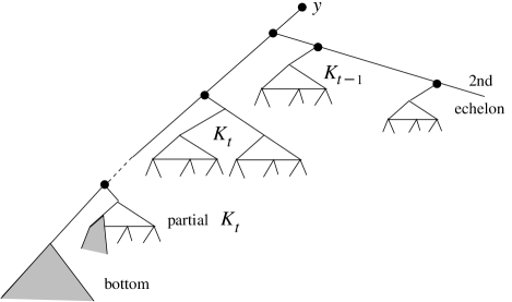
Figure 13: The clusters in $\text{\rm fetch}(t,M_{h}^{[2]})$, given $t<\text{\rm irp}(M_{h}^{[2]}$).

Below the left and right depth of nodes in a tree are defined. This will enable us to prove an important bound on the length of extensions in traversing a cluster.

Definition 30

The depth of a node $q$ in a tree $T$ is, of course, the number of proper ancestors of $q$. Here we define left and right depths.

Paradoxically, left depth counts right ancestors and vice-versa.

A right (respectively, left) ancestor of $q$ is a node whose left (respectively, right) subtree contains $q$. The left depth of $q$ is the number of right ancestors and the right depth is the number of left ancestors.

Thus the depth is the sum of left and right depths. If a node is on the spine, then its left depth is the number of nodes above it on the spine.

Lemma 31

(i) Fetch-and-discard on any tree $T$ does not increase the left depth of any node. (ii) if $T=C^{[2]}$ where $C$ is a cluster, fetch does not increase the number of right ancestors which are $x$-nodes.

Proof. (i) Let $q$ be a node before the fetch. If $q$ is leftmost then it is fetched and (implicitly) the result follows automatically. So we assume that $q$ is not leftmost in $T$.

• If $q\notin\text{\rm spine}(T)$, say it is in the right subtree $R$ of a spine node $p$. Let $S$ be that part of $\text{\rm spine}(T)$ above $p$.

• If $q\notin\text{\rm spine}(T)$ and $p$ is leftmost and fetched, $R$ will be attached to a subsequence of $S$ which brings $q$ closer to the root of $\text{\rm fetch}(1,T)$.

• If $q\notin\text{\rm spine}(T)$ and $p$ is not leftmost and not pushed off the spine, then $p$ is brought closer to the root and so is $q$.

• If $q\in\text{\rm spine}(T)$ and $q$ is pushed off the spine by another node $p$, then $q$ acquires a new ancestor $p$, but it is a left ancestor.

• If $q\in\text{\rm spine}(T)$ and is not pushed off the spine, then it is no further from the root after than before the fetch.

(ii): similarly.      

Corollary 32

Let $C=K_{t-1}(M_{h}^{[2]})$ be a cluster. Suppose that after $f$ fetches, $A_{i}$ is attached to the spine, i.e., the root of $A_{i}$ is on $\text{\rm spine}(\text{\rm fetch}(f,C^{[2]}))$. Let $E$ be the set of spine nodes above this root. Then $|E|\leq t+1$.      

Lemma 33

When $A=M_{h}$, the $t$-base $D$ (Definition 28) has size $|D|\leq 2t-1$. Left subtrees of nodes on the second echelon which contain only nodes from $D$ have size $\leq|D|$. In a partial cluster, there are at most $|D|$ nodes from $D$ (Obviously).      

Figure 14: parts of $C^{[2]}$ (see Lemma 35).

Figure 15: A regular tree $C^{\prime}$.

.

In the lemma below, $t$, and $t\leq\log_{2}(h+3)$, will be replaced at one point by $h$, which is assumed to be no smaller. But $h\geq\log_{2}(h+3)$ is only valid for $h\geq 3$. So, consider $0,1,2$ separately.

Lemma 34

$${\text{\rm rp}}(M_{0}^{[2]}=2,{\text{\rm rp}}(M_{1}^{[2]}=4,~{}\text{\rm and}~{}{\text{\rm rp}}(M_{2}^{[2]}=2.$$

Sketch proof. See Figure 7 for ${\text{\rm rp}}(M_{1}^{[2]})$; check that $\text{\rm irp}(M_{1}^{[2]})=1$; ${\text{\rm rp}}(M_{0}^{[2]}$ is easily checked.

Lemma 35

If $C$ is a $t$-cluster, or partial cluster, or pseudo-cluster, derived as part of the fetch-and-discard traversal of $M_{h}^{[2]}$, then

$${\text{\rm rp}}(C^{[2]})\leq 14\log_{2}^{2}(4(h+1))+2|X|\log_{2}(4(h+1))$$

where $X$ is the set of $x$-nodes in $C$.

Proof. We divide $C$ into four parts, $D,U,I,R$ as in Figure 14. Usually all but the last will be empty.

The argument is based on the facts that $D$ is small, $U$ is small ($U$ is based on an index $i_{0}$ where $h-i_{0}$ is small), $I$ does not contribute to the root persistence, and the base trees $A_{i}$ are sufficiently large to admit Lemma 24.

(i) $D$ consists of all nodes in the $t$-base. An obvious upper bound for the cost of traversing $D$ is $|D|^{2}$ which is less than $4t^{2}$. Since this counts all steps whether or not $y$ is at the root, it gives an upper bound for the contribution of these steps to ${\text{\rm rp}}(C^{[2]})$.

Let $C^{\prime}=\text{\rm fetch}(|D|,C^{[2]})$. Once $D$ is fetched, $C^{\prime}$ is regular, meaning that it consists of an upper part formed of $x$-nodes, with subtrees $A_{i}$ attached to it (Figure 15).

Let $E$ be the $x$-nodes (plus $y$ if it is on the spine) on the spine of $C^{\prime}$, and $A_{i}$ the leftmost $A$-tree, so $A_{i}^{[E]}$ is part of $C^{\prime}$ and $|E|\leq t+1$ (Corollary 32).

Now, $A_{i}=M_{h-i-1}$ with height $h-i-1$. Let $k=2\lceil\log_{2}(h-i+|E|)\rceil-1$.

From Lemma 24, if $k\leq|A_{i}|$ then within at most $k$ steps the spine is reduced to a single node, and either that node is $y$, the only node left, or it isn’t and $y$ has been pushed off the spine (see Corollary 25).

(ii) The set $U$ allows for the possibility that $k>|A_{i}|$. We focus on those subtrees $A_{i}$, the $A$-subtrees, which are attached to the regular tree $C^{\prime}$.

If $k>|A_{i}|$ then

$$2\lceil\log_{2}(h-i+|E|)\rceil>2^{h-i}-1$$

$$\lceil\log_{2}(h-i+|E|)\rceil\geq 2^{h-i-1}$$

$$\log_{2}(h-i+|E|)>2^{h-i-1}-1$$

The above condition implies the simpler condition

$$\log_{2}(h+t+1)>2^{h-i-1}-1.$$

and we define $U$ by this condition, which may include more of $C^{\prime}$ than is necessary, but leaves nothing out.

If $A_{i}\in U$ and $i^{\prime}>i$ then $A_{i^{\prime}}\in U$. So let $i_{0}$ be the smallest $i$ satisfying

$$\log_{2}(h+t+1)>2^{h-i-1}-1$$

$$2^{h-i-1}<\log_{2}(h+t+1)+1=\log_{2}(2(h+t+1))$$

$$h-i-1<\log_{2}\log_{2}(2(h+t+1))$$

$$i>h-1-\log_{2}\log_{2}(2(h+t+1))$$

$$i_{0}$$ is minimal:

$$i_{0}=1+\lfloor h-1-\log_{2}\log_{2}(2(h+t+1))\rfloor$$

$$i_{0}=\lfloor h-\log_{2}\log_{2}(2(h+t+1))\rfloor$$

The indices $i$ are decreasing and bounded above by $h$. For each index $i$, there is the tree $A_{i}$, and the successor $x$-node, in $U$. The range of values for $i\geq i_{0}$ is at most

$$\{i:h-i_{0}\leq i\leq h\}$$

The total number of nodes in $U$ is bounded by

$$\sum_{i_{0}}^{h}(1+|A_{i}|)=\sum 2^{h-i}<2^{h-i_{0}+1}\leq 4\log_{2}(2(h+t+1))$$

The cost of fetching a node in $U$ is bounded by $t+1+h-i_{0}+1$, i.e.,

$$t+2+\lceil\log_{2}\log_{2}(2(h+t+1))\rceil$$

Therefore the total cost of fetching all the nodes in $U$ is at most

$$4\log_{2}(2(h+t+1))\times(t+2+\lceil\log_{2}\log_{2}(2(h+t+1))\rceil)$$

This is an upper bound on the contribution of $U$ to ${\text{\rm rp}}(C^{[2]})$.

(iii) The part $I$ allows for $y$ to be restored to the spine in case after fetching $D$ and $U$ it has been pushed off the spine. There is no contribution to the root persistence of $C^{[2]}$.

(iv) Given $C^{\prime}=\text{\rm fetch}(|D|+|U|+|I|,C^{[2]})$, $C^{\prime}$ is regular, and $y$ is on the spine. Suppose that $A_{i}$ is the $A$-subtree aligned with the spine, and $E$ is the remainder of the spine. Within at most $k=2\lceil\log_{2}(h-i+|E|)\rceil-1$ fetches, since this time $k$ is not too large, $y$ is pushed off the spine.

This contributes less than $2\lceil\log_{2}(h+t+1)\rceil$ to the root persistence of $C^{[2]}$.

After a certain number of fetches, which do not contribute to the root persistence, $y$ is restored to the spine, by a fetch which removed one of the $x$-nodes.

So this process repeats at most $|X|$ times, where $X$ is the number of $x$-nodes in $C^{[2]}$, and the overall root persistence in traversing $R$ (see Figure 14) is bounded by

$$2|X|\lceil\log_{2}(h+t+1)\rceil$$

The total estimate is as follows.

$${\text{\rm rp}}(C^{[2]})\leq 4t^{2}+$$

$$4\log_{2}(2(h+t+1))\times(t+2+\lceil\log_{2}\log_{2}(2(h+t+1))\rceil)+$$

$$2|X|\lceil\log_{2}(h+t+1)\rceil.$$

To simplify this we make some observations.

$$1\leq t<\text{\rm irp}(M_{h}^{[2]})\leq\lceil\log_{2}(h+3)\rceil$$

$$\log_{2}(h+3)\leq\log_{2}(2(h+t+2))$$

$$\text{if}~{}x\geq 2,\quad\lceil\log_{2}x\rceil\leq x$$

$$\log_{2}(2(h+t+1))\geq 2$$

$$\lceil\log_{2}\log_{2}(2(h+t+1))\rceil\leq\log_{2}(2(h+t+1))\leq\log_{2}(2(h+t+2)).$$

so

$${\text{\rm rp}}(C^{[2]}\leq 4(\log_{2}^{2}(2(h+t+2))+$$

$$4\log_{2}(2(h+t+2))\times(\log_{2}(2(h+t+2))+2+\log_{2}(2(h+t+2))+$$

$$2|X|\log_{2}(2(h+t+2)).$$

The root persistence of $M_{h}^{[2]}$ for $h=0,1,2,$ is known (Lemma 34): $2,4,2$. Assuming $h\geq 3$, $t\leq h$ and we replace $h+t$ by $2h$.

$${\text{\rm rp}}(C^{[2]}\leq 4(\log_{2}^{2}(4(h+1))+$$

$$4\log_{2}(4(h+1))\times(\log_{2}(4(h+1))+2+\log_{2}(4(h+1))+$$

$$2|X|\log_{2}(4(h+1))=$$

$$12\log_{2}^{2}(4(h+1))+8\log_{2}(4(h+1))+2|X|\log_{2}(4(h+1))$$

(36) $${\text{\rm rp}}(C^{[2]})\leq 14\log_{2}^{2}(4(h+1))+2|X|\log_{2}(4(h+1)).$$

(This is obviously true when $h\leq 2$.)      

Adding these for $1\leq t\leq 2\log_{2}(h+3)$, the sets $X$ are disjoint and have total size $\leq h+2$, so

Corollary 37

$${\text{\rm rp}}(M_{h}^{[2]})\leq 14\log_{2}^{2}(4(h+1))(h+3)+2(h+2)\log_{2}(4(h+1))\leq$$

$$(h+3)(14\log_{2}^{2}(4(h+1))+2\log_{2}(4(h+1))\leq$$

$$15(h+3)\log_{2}^{2}(4(h+1))$$

From Corollary 19,

$${\text{\rm rp}}(M_{h}^{[1]}\leq\sum_{j<h}15(j+3)\log_{2}^{2}(4(j+1))\leq 15\log_{2}^{2}(4(h+1))(h+3)(h+2)/2$$

$$\leq 8(\log_{2}(h+3)+2)^{2}(h+3)^{2}$$

Now, the estimates of $M_{h}^{[2]}$ were needed for all $h\geq 0$, but we may assume $\log_{2}(h+3)+2\leq h+3$ without further investigation since we need estimates of $M_{h}^{[1]}$ only for large $h$. Therefore

Corollary 38

For almost all $h$,

$${\text{\rm rp}}(M_{h}^{[1]})\leq 8(h+3)^{4}.\nobreak\hskip 0.0pt\hskip 15.00002pt minus 5.0pt\nobreak\vrule height=7.5pt,width=5.0pt,depth=2.5pt$$

Lemma 39

$$\sum_{n\geq N}\frac{n^{4}}{2^{n}}=\frac{N^{4}+4N^{3}+18N^{2}+52N+75}{2^{N-1}}\leq\frac{(N+3)^{4}}{2^{N-1}}$$

The equation can be derived easily by assuming that the sum is a quartic in $N$ divided by $2^{N}$, and applying the method of undetermined coefficients.      

Corollary 40

For any $N>1$,

$$\alpha\leq\alpha_{N-1}+8\frac{(N+3)^{4}}{2^{N-1}}.\nobreak\hskip 0.0pt\hskip 15.00002pt minus 5.0pt\nobreak\vrule height=7.5pt,width=5.0pt,depth=2.5pt$$

References

1. Amr Elmasry (2004). On the sequential access conjecture and deque conjecture for splay trees. Theoretical Computer Science 314:3, 459–466.

2. Simon Kristensen (2017). Arithmetic properties of series of reciprocals of algebraic integers. Talk delivered to the Department of Mathematics, Maynooth University, 27 March 2017.

3. Daniel Sleator and Robert E. Tarjan (1985). Self-adjusting binary search trees. Journal Assoc. Computing Machinery 32:3, 652–686.

4. Robert E. Tarjan (1985). Sequential access in splay trees takes linear time. Combinatorica 5:4, 367–378.