EDA: EXAFS Data Analysis software package

Abstract

The EXAFS data analysis software package EDA consists of a suite of programs running under Windows operating system environment and designed to perform all steps of conventional EXAFS data analysis such as the extraction of the XANES/EXAFS parts of the x-ray absorption coefficient, the Fourier filtering, the EXAFS fitting using the Gaussian and cumulant models. Besides, the package includes two advanced approaches, which allow one to reconstruct the radial distribution function (RDF) from EXAFS based on the regularization-like method and to calculate configurational-averaged EXAFS using a set of atomic configurations obtained from molecular dynamics or Monte Carlo simulations.

1 General concept

Below the EXAFS data analysis software package EDA [EDA] is described in details emphasising its key features. The full package, documentation and application examples are available for download at http://www.dragon.lv/eda/.

The EDA package has been under continuous development from 1988. It has been created with an idea to be intuitively simple and fast, guiding the user step by step through each part of the EXAFS analysis. Originally developed for the MS-DOS compatible operating systems, the current version of the package consists of a set (Table 1) of interactive programs running under Windows operating system environment. The originality of the EDA package is mainly related to (i) the procedure of the EXAFS oscillation extraction from the experimental data performed by the EDAEES code, (ii) the regularization-like method for the radial distribution function (RDF) reconstruction from EXAFS by the EDARDF code [EDARDF] and (iii) the calculation of configuration-averaged EXAFS based on the results of molecular dynamics or Monte Carlo simulations by the EDACA code [Kuzmin2009].

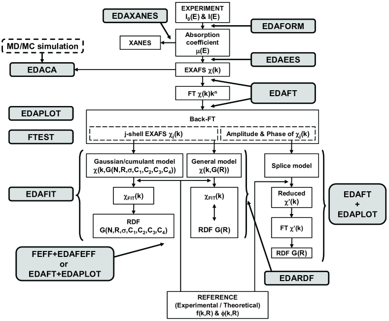
Figure 1: Flowchart of the EXAFS data analysis by the EDA package.

The various components of the EDA package and their relation are shown in Fig. 1, where the main steps of the analysis and the computer codes involved are given. We will describe it briefly below.

When performing XAS experiment, one usually obtains two signals $I_{0}(E)$ and $I(E)$, which are proportional to the intensity of the X-ray beam with the energy $E$ before and after interaction with the sample. These two signals are used to calculated the X-ray absorption coefficient $\mu(E)$ by the EDAFORM code.

At this point, the X-ray absorption near edge structure (XANES) of $\mu(E)$ can be isolated and analysed by calculating its first and second derivatives using the EDAXANES code. This step allows one to determine precisely the position of the absorption edge and, thus, to check the reproducibility of the energy scale for the single sample or to determine the absorption edge shift $\Delta E$ due to a variation of the effective charge of the absorbing atom in different compounds.

The extraction of the EXAFS $\chi(E)=(\mu(E)-\mu_{b}(E)-\mu_{0}(E))/\Delta\mu_{0}(E)$ is implemented in the EDAEES code using the following sophisticated procedure. The background contribution $\mu_{b}(E)$ is determined by extrapolating the pre-edge background as $\mu_{b}(E)=A-B/E^{3}$. Next, the atomic-like contribution $\mu_{0}(E)$ is determined as $\mu_{0}(E)=\mu_{0}^{I}(E)+\mu_{0}^{II}(k)+\mu_{0}^{III}(k)$, where the three functions $\mu_{0}^{I}(E)=P_{n}(E)$, $\mu_{0}^{II}(k)=P_{m}(k)$ ($P_{n}$ is the polynomial of n-order) and $\mu_{0}^{III}(k)=S_{3}(k,p)$ ($S_{3}(k,p)$ is the smoothing cubic spline with the parameter $p$) are calculated in series, the first one in $E$-space whereas the last two in $k$-space ($k$ is the photoelectron wavenumber). The EXAFS normalization is performed as $\Delta\mu_{0}(E)=\mu_{0}^{I}(E)$. Such procedure guarantees accurate determination of the $\mu_{0}(E)$ function, and as a result, the EXAFS $\chi(k)$, even if experimental data are far from ideal. The $k$ scale is conventionally defined as $k=\sqrt{(2m_{e}/\hbar^{2})(E-E_{0})}$, where $m_{e}$ is the electron mass, $\hbar$ is the Planck’s constant, and $E_{0}$ is the threshold energy, i.e., the energy of a free electron with zero momentum. Deglitching and normalization of the EXAFS to the edge jump $\Delta\mu_{0}(E)$ obtained from the reference compound, theoretical tables [Teo1986] or equal to a constant are also possible.

The extracted experimental EXAFS $\chi(k)$ can be directly compared with the configuration-averaged EXAFS calculated based on the results of molecular dynamics (MD) or Monte Carlo (MC) simulations by the EDACA code or can be analysed in more conventional way. In the latter case, the Fourier filtering procedure (i.e. direct and back Fourier transforms (FTs) with some suitable ”window”-function) is applied using the EDAFT code to separate a contribution from the required range in $R$-space into the total EXAFS. Such approach allows one to simplify the analysis, at least, for a contribution from the first coordination shell of the absorbing atom.

Finally, the EXAFS from a single or several coordination shells can be simulated using different models to extract structural information. The EDA package allows one to use three models (the first two will be discussed below): (i) conventional multi-component parameterized model within the Gaussian or cumulant approximation (the EDAFIT code, see Section 2), (ii) arbitrary RDF model determined by the regularization-like approach (the EDARDF code, see Section 3), (iii) the so-called ”splice” model [stern92] (combined use of the EDAFT and EDAPLOT codes is required). To perform simulations, one needs to provide the scattering amplitude $f(k,R)$  and phase shift $\phi(k,R)$ functions for each scattering path. These data can be obtained from experimental EXAFS spectrum of some reference compound, taken from tables [Teo1986, McKale1988] or calculated theoretically. In the EDA package, one has possibility to use the theoretical data calculated by the FEFF8/9 codes [FEFF8, FEFF9], which can be extracted from the feff****.dat files by the EDAFEFF code.

Finally, the EDAPLOT code is provided for visualization, comparison and simple mathematical analysis of any data obtained within the EDA package. Note that since all data are kept in simple ASCII format, they can be easily imported to and treated by any other codes.

2 Multi-component model within the Gaussian/cumulant approximation.

The fitting of the EXAFS $\chi(k)$ in the $k$-space within the single-scattering curved-wave approximation is implemented in the EDAFIT code which is based on the cumulant expansion of the EXAFS equation [Rehr2000, Kuzmin2014IUCR]

$$\chi(k) = \sum_{i}^{shells}S_{0}^{2}{{N_{i}}\over{kR^{2}_{i}}}f_{i}(\pi,k,R_{i})\exp(-2\sigma_{i}^{2}k^{2}+{2\over 3}C_{4i}k^{4}$$ (1)

$$- {4\over 45}C_{6i}k^{6})\exp(-2R_{i}/\lambda(k))\sin(2kR_{i}-{4\over 3}C_{3i}k^{3}$$

$$+ {4\over 15}C_{5i}k^{5}+\phi_{i}(\pi,k,R_{i}))$$

where $k=\sqrt{k^{\prime 2}+(2m_{e}/\hbar^{2})\Delta E_{0i}}$ is the photoelectron wavenumber corrected for the difference $\Delta E_{0i}$ in the energy origin between experiment and theory; $S_{0}^{2}$  is the scale factor taking into account amplitude damping due to multielectron effects; $N_{i}$  is the coordination number of the i-th shell; $R_{i}$  is the radius of the i-th shell; $\sigma_{i}$  is the mean-square relative displacement (MSRD) or Debye-Waller factor; $C_{3i}$, $C_{4i}$, $C_{5i}$ and $C_{6i}$ are cumulants of a distribution taking into account anharmonic effects and/or non-Gaussian disorder; $\lambda(k)=k/\Gamma$  ($\Gamma$ is a constant) is the mean free path (MFP) of the photoelectron; $f(\pi,k,R_{i})$  is the backscattering amplitude of the photoelectron due to the atoms of the i-th shell; $\phi(\pi,k,R_{i})=\psi(\pi,k,R_{i})+2\delta_{l}(k)-l\pi$ is the phase shift containing contributions from the absorber $2\delta_{l}(k)$ and the backscatterer $\psi(\pi,k,R_{i})$ ($l$ is the angular momentum of the photoelectron).

The fitting parameters of the model are $S_{0}^{2}N_{i}$, $R_{i}$, $\sigma^{2}_{i}$, $\Delta E_{0i}$, $C_{3i}$, $C_{4i}$, $C_{5i}$, $C_{6i}$ and $\Gamma$. The maximum number of fitting parameters, which can be used in the EXAFS model, is limited by the Nyquist criterion $N_{\rm par}=2\Delta k\Delta R/\pi$ [Stern1993].

Note that when the functions $f(\pi,k,R_{i})$  and $\phi(\pi,k,R_{i})$ are extracted from the EXAFS spectrum of a reference compound, the values of fitting parameters will be relative. To compare different models obtained by fitting of the EXAFS using the EDAFIT code, Fisher’s $F_{0.95}$ criterion, implemented in the FTEST code [EDA], can be applied.

3 Regularization-like method

The regularization-like method implemented in the EDARDF code allows one to determine model independent RDF $G(R)$ from the experimental EXAFS. It is especially suitable for the analysis of the first coordination shell in locally distorted or disordered materials, such as low-symmetry crystals (e.g. with Jahn-Teller distortions), amorphous compounds, glasses, and systems with strongly anharmonic behaviour, where a decomposition into the cumulant series fails. At the same time, the method can be also used in more simple cases as a starting point for the selection of a conventional model described in the previous section.

The RDF $G(R)$ is determined by inversion of the EXAFS equation within the single-scattering approximation

$$\chi(k)=S_{0}^{2}\int_{R_{\rm{min}}}^{R_{\rm{max}}}{{G(R)}\over{kR^{2}}}f(\pi,k,R)\sin(2kR+\phi(\pi,k,R))dR$$ (2)

using the iterative method described in [Kuzmin2000]. Two regularizing criteria are applied after each iteration to restrict the shape of $G(R)$ to physically significant solutions: it must be positive-defined and smooth function.

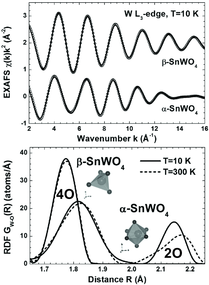
Figure 2: Upper panel: comparison of the experimental (circles) and calculated (solid lines) W L₃-edge EXAFS spectra $\chi(k)k^{2}$ for the first coordination shell of tungsten in $\alpha$-SnWO₄ (lower curves) and $\beta$-SnWO₄ (upper curves) at 10 K. Lower panel: calculated radial distribution functions (RDF’s) $G_{\rm W-O}(R)$ for W–O bonds within the first coordination shell of tungsten in $\alpha$-SnWO₄ and $\beta$-SnWO₄ at 10 K (solid lines) and 300 K (dashed lines). The two groups of 4 and 2 oxygen atoms are indicated.

The use of the method is demonstrated in Fig. 2 for the case of tin tungstate, which exists in two phases – $\alpha$-SnWO₄ and $\beta$-SnWO₄ [Kuzmin2015]. In orthorhombic $\alpha$-SnWO₄ phase tungsten atoms are six-fold coordinated by oxygen atoms, and the WO₆ octahedra are strongly distorted due to the second-order Jahn-Teller effect because of the W⁶⁺(5$d^{0}$) electronic configuration. The six W–O bonds in $\alpha$-SnWO₄ are split into two groups of four short bonds at $\sim$1.82 Å and two long bonds at $\sim$2.15 Å. In cubic $\beta$-SnWO₄ tungsten atoms have slightly deformed WO₄ tetrahedral coordination with the W–O bond lengths of about 1.77 Å. An increase of temperature from 10 K to 300 K affects weakly the W–O bonding in the WO₄ tetrahedra and also the group of four shortest W–O bonds in the WO₆ octahedra. At the same time, the distant group of weakly bound two oxygen atoms in the WO₆ octahedra shifts to longer distances and becomes more broadened. Thus, the reconstructed RDFs reproduce nicely the W L₃-edge EXAFS in both tin tungstates and allow one to follow a distortion of the tungsten first shell in details.

Another example, shown in Fig. 2, is concerned the local atomic structure relaxation upon crystallite size reduction in ZnWO₄ [Kalinko2011]. Crystalline ZnWO₄ has monoclinic ($P2/c$) wolframite-type structure built up of distorted WO₆ and ZnO₆  octahedra joined by edges into infinite zigzag chains. The distortion of the metal-oxygen octahedra leads to the splitting of the W–O and Zn–O distances into three groups of two oxygen atoms each with the bond lengths of about 1.79, 1.91 and 2.13 Å around tungsten atoms and 2.03, 2.09 and 2.22 Å around zinc atoms. Note that the three W–O groups are well resolved in the RDF. Upon the reduction of crystallite size down to $\sim$2 nm, significant relaxation of the atomic structure occurs leading to some broadening of the RDF peaks, especially at large distances (2.1-2.4 Å), whereas the nearest oxygen atoms become stronger bound. Such structural changes in ZnWO₄ nanoparticles correlate with their optical and vibrational properties.

Other application examples of the method include dehydration process in molybdenum oxide hydrate [Kuzmin2000], the effect of composition and crystallite size reduction in tungstates [Kuzmin2001, Anspoks2014b, Kuzmin2014], and studies of the local environment in glasses [Kuzmin1997a, Rocca1998, Rocca1999, Kuzmin2006].

4 Configuration-averaged EXAFS simulations

A particular feature of the EDA package is its ability to perform more advanced calculations of the configuration-averaged EXAFS based on the results of MD simulations (Fig. 4) [Kuzmin2009, Kuzmin2014IUCR, Kuzmin2016val]. Note that a set of atomic configurations generated using the MC simulation [PIMC2008] can be also used in a similar manner. To use this approach, called MD-EXAFS, one needs to provide an *.XYZ file containing temporal snapshots of atomic coordinates, which can be obtained from most MD codes such as GULP [Gale2003], DLPOLY [DLPOLY], LAMMPS [LAMMPS1995] or CP2K [VandeVondele2005]. Additionally the input file with a set of commands for the FEFF8/9 code is also required.

A care should be taken to get proper configuration-averaged EXAFS. This means that a number of snapshots should be sufficiently large (usually few thousands) to get good statistics, and the time step between subsequent snapshots should be enough small to sample properly the dynamic properties of the material. The MD-EXAFS approach allows one to validate different theoretical models, e.g. force-fields, and/or perform the EXAFS interpretation far beyond the nearest coordination shells.

Application examples of this method cover several compounds: SrTiO₃ [Kuzmin2009], ReO₃ [Kalinko2009jpcs], Ge [Timoshenko2011], NiO [Anspoks2010, Anspoks2012, Anspoks2014], LaCoO₃ [Kuzmin2011], ZnO [Timoshenko2014zno], AWO₄ (A=Ca, Sr, Ba) tungstates [Kalinko2016], Y₂O₃ [Jonane2016y2o3], FeF₃ [Jonane2016fef3] and UO₂ [Bocharov2017].

The case of microcrystalline and nanocrystaline (6 nm) NiO [Anspoks2012] is illustrated in Fig. 5. The Ni K-edge EXAFS spectra of both compounds are dominated by a contribution from the first two coordination shells (Ni–O₁ and Ni–Ni₂) of nickel. However, the outer shells are responsible for a number of well resolved peaks located above $\sim$3 Å in the Fourier transforms. Due to cubic rock-salt structure of NiO, the multiple-scattering events play an important role in the formation of EXAFS and must be treated properly. The classical MD simulations [Anspoks2012] were performed using the force-field model included two-body central force interactions between atoms described by a sum of the Buckingham and Coulomb potentials. The effects of crystallite size, thermal disorder and Ni vacancy concentration were taken into account. The calculated configuration-averaged EXAFS reproduces well the experimental data for both nickel oxides. In the case of nanocrystalline NiO, the damping of the EXAFS oscillations due to the atomic structure relaxation and the progressive decrease of the FT peaks amplitude at longer distances are observed as a result of the crystallite size reduction.

This work was supported by the Latvian Science Council grant no. 187/2012.

5 References

Table 1: A set of programs for EXAFS data analysis and simulations included in the EDA software package.

Code title	Code description
EDAFORM	converts original experimental data from several beamlines into
	the EDA file format (ASCII, 2 columns).
EDAXANES	extracts the XANES part of the experimental X-ray absorption
	spectrum and calculates its first and second derivatives.
EDAEES	extracts the EXAFS part $\chi(k)$ using original algorithm for the
	atomic-like (”zero-line”) background removal.
EDAFT	performs Fourier filtering procedure (direct and back Fourier
	transforms) with or without amplitude/phase correction using
	a number of different (rectangular, Gaussian, Kaiser-Bessel,
	Hamming and Norton-Beer F3) window functions.
EDAFIT	is a non-linear least-squares fitting code, based on a high speed
	algorithm without matrix inversion. A multi-shell Gaussian or
	cumulant model within the single-scattering approximation can
	contain up to 20 shells with up to 8 fitting parameters ($N_{i}$, $S_{o}^{2}$,
	$R_{i}$, $\sigma_{i}^{2}$, $\Delta E_{0i}$, $C_{3i}$, $C_{4i}$, $C_{5i}$, $C_{6i}$) in each. Constrains on the range
	of any fitting parameter or its value can be imposed.
EDARDF	is the regularization-like least-squares-fitting code allowing one
	to determine model-independent RDF in the first coordination
	shell for a compound with arbitrary degree of disorder.
FTEST	performs analysis of variance of the fitting results based on
	the Fisher’s $F_{0.95}$-test.
EDAPLOT	is a general-purpose program for plotting, comparison, and
	mathematical calculations frequently used in the EXAFS data
	analysis (more than 20 different operations).
EDAFEFF	extracts the scattering amplitude and phase shift functions from
	FEFF****.dat files, calculated by the FEFF8/9 code, for the use
	with the EDAFIT or EDARDF codes.
EDACA	calculates configuration-averaged EXAFS based on the results
	of molecular dynamics simulations.

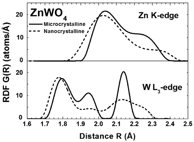
Figure 3: The reconstructed RDFs $G(R)$ for the first coordination shell of tungsten and zinc in nanoparticles and microcrystalline ZnWO₄.

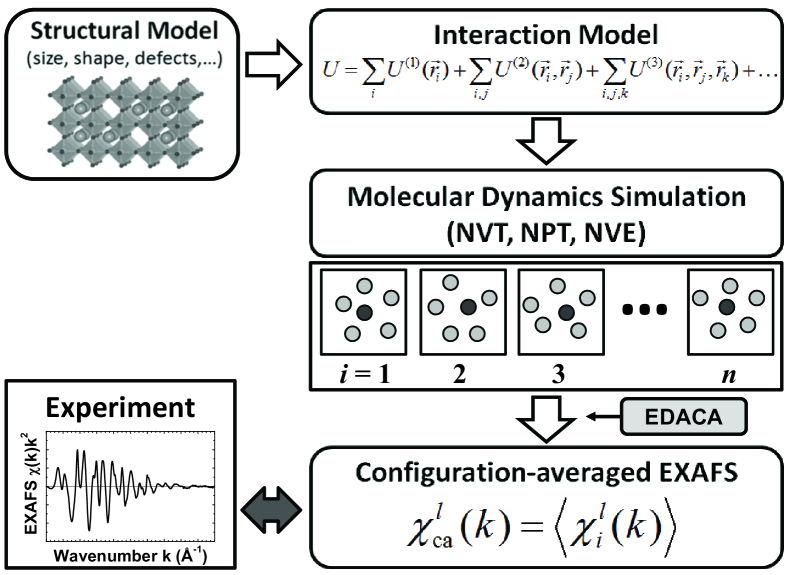
Figure 4: Flowchart of the MD-EXAFS calculations.

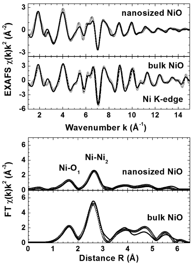
Figure 5: Comparison of the experimental (circles) and calculated configuration-averaged (solid lines) Ni K-edge EXAFS spectra $\chi(k)k^{2}$ (upper panel) and their Fourier transforms (lower panel) for bulk and nanosized NiO at 300 K.

References

- [1] \harvarditema Beccara \harvardand Fornasini2008PIMC2008 a Beccara, S. \harvardand Fornasini, P. \harvardyearleft2008\harvardyearright. Phys. Rev. B, \volbf77, 172304.
- [2] \harvarditem[Ankudinov et al.]Ankudinov, Ravel, Rehr \harvardand Conradson1998FEFF8 Ankudinov, A. L., Ravel, B., Rehr, J. J. \harvardand Conradson, S. D. \harvardyearleft1998\harvardyearright. Phys. Rev. B, \volbf58, 7565–7576.
- [3] \harvarditem[Anspoks et al.]Anspoks, Kalinko, Kalendarev \harvardand Kuzmin2012Anspoks2012 Anspoks, A., Kalinko, A., Kalendarev, R. \harvardand Kuzmin, A. \harvardyearleft2012\harvardyearright. Phys. Rev. B, \volbf86, 174114.
- [4] \harvarditem[Anspoks et al.]Anspoks, Kalinko, Kalendarev \harvardand Kuzmin2014aAnspoks2014 Anspoks, A., Kalinko, A., Kalendarev, R. \harvardand Kuzmin, A. \harvardyearleft2014a\harvardyearright. Thin Solid Films, \volbf553, 58–62.
- [5] \harvarditem[Anspoks et al.]Anspoks, Kalinko, Timoshenko \harvardand Kuzmin2014bAnspoks2014b Anspoks, A., Kalinko, A., Timoshenko, J. \harvardand Kuzmin, A. \harvardyearleft2014b\harvardyearright. Solid State Commun. \volbf183, 22–26.
- [6] \harvarditem[Anspoks et al.]Anspoks, Kuzmin, Kalinko \harvardand Timoshenko2010Anspoks2010 Anspoks, A., Kuzmin, A., Kalinko, A. \harvardand Timoshenko, J. \harvardyearleft2010\harvardyearright. Solid State Commun. \volbf150, 2270–2274.
- [7] \harvarditem[Bocharov et al.]Bocharov, Chollet, Krack, Bertsch, Grolimund, Martin, Kuzmin, Purans \harvardand Kotomin2017Bocharov2017 Bocharov, D., Chollet, M., Krack, M., Bertsch, J., Grolimund, D., Martin, M., Kuzmin, A., Purans, J. \harvardand Kotomin, E. \harvardyearleft2017\harvardyearright. Prog. Nucl. Energy, \volbf94, 187–193.
- [8] \harvarditemGale \harvardand Rohl2003Gale2003 Gale, J. D. \harvardand Rohl, A. L. \harvardyearleft2003\harvardyearright. Mol. Simul. \volbf29, 291–341.
- [9] \harvarditem[Jonane et al.]Jonane, Lazdins, Timoshenko, Kuzmin, Purans, Vladimirov, Gräning \harvardand Hoffmann2016aJonane2016y2o3 Jonane, I., Lazdins, K., Timoshenko, J., Kuzmin, A., Purans, J., Vladimirov, P., Gräning, T. \harvardand Hoffmann, J. \harvardyearleft2016a\harvardyearright. J. Synchrotron Rad. \volbf23, 510–518.
- [10] \harvarditem[Jonane et al.]Jonane, Timoshenko \harvardand Kuzmin2016bJonane2016fef3 Jonane, I., Timoshenko, J. \harvardand Kuzmin, A. \harvardyearleft2016b\harvardyearright. Phys. Scr. \volbf91, 104001.
- [11] \harvarditem[Kalinko et al.]Kalinko, Bauer, Timoshenko \harvardand Kuzmin2016Kalinko2016 Kalinko, A., Bauer, M., Timoshenko, J. \harvardand Kuzmin, A. \harvardyearleft2016\harvardyearright. Phys. Scr. \volbf91, 114001.
- [12] \harvarditem[Kalinko et al.]Kalinko, Evarestov, Kuzmin \harvardand Purans2009Kalinko2009jpcs Kalinko, A., Evarestov, R., Kuzmin, A. \harvardand Purans, J. \harvardyearleft2009\harvardyearright. J. Phys.: Conf. Series, \volbf190, 012080.
- [13] \harvarditemKalinko \harvardand Kuzmin2011Kalinko2011 Kalinko, A. \harvardand Kuzmin, A. \harvardyearleft2011\harvardyearright. J. Non-Cryst. Solids, \volbf357, 2595–2599.
- [14] \harvarditemKuzmin1995EDA Kuzmin, A. \harvardyearleft1995\harvardyearright. Physica B, \volbf208-209, 175–176.
- [15] \harvarditemKuzmin1997EDARDF Kuzmin, A. \harvardyearleft1997\harvardyearright. J. Physique IV (France), \volbf7, C2–213–C2–214.
- [16] \harvarditem[Kuzmin et al.]Kuzmin, Anspoks, Kalinko \harvardand Timoshenko2016Kuzmin2016val Kuzmin, A., Anspoks, A., Kalinko, A. \harvardand Timoshenko, J. \harvardyearleft2016\harvardyearright. Z. Phys. Chem. \volbf230, 537–549.
- [17] \harvarditem[Kuzmin et al.]Kuzmin, Anspoks, Kalinko, Timoshenko \harvardand Kalendarev2014Kuzmin2014 Kuzmin, A., Anspoks, A., Kalinko, A., Timoshenko, J. \harvardand Kalendarev, R. \harvardyearleft2014\harvardyearright. Phys. Scr. \volbf89, 044005.
- [18] \harvarditem[Kuzmin et al.]Kuzmin, Anspoks, Kalinko, Timoshenko \harvardand Kalendarev2015Kuzmin2015 Kuzmin, A., Anspoks, A., Kalinko, A., Timoshenko, J. \harvardand Kalendarev, R. \harvardyearleft2015\harvardyearright. Sol. Energy Mater. Sol. Cells, \volbf143, 627–634.
- [19] \harvarditemKuzmin \harvardand Chaboy2014Kuzmin2014IUCR Kuzmin, A. \harvardand Chaboy, J. \harvardyearleft2014\harvardyearright. IUCrJ, \volbf1, 571–589.
- [20] \harvarditem[Kuzmin et al.]Kuzmin, Dalba, Fornasini, Rocca \harvardand Šipr2006Kuzmin2006 Kuzmin, A., Dalba, G., Fornasini, P., Rocca, F. \harvardand Šipr, O. \harvardyearleft2006\harvardyearright. Phys. Rev. B, \volbf73, 174110.
- [21] \harvarditem[Kuzmin et al.]Kuzmin, Efimov, Efimova, Sikolenko, Pascarelli \harvardand Troyanchuk2011Kuzmin2011 Kuzmin, A., Efimov, V., Efimova, E., Sikolenko, V., Pascarelli, S. \harvardand Troyanchuk, I. O. \harvardyearleft2011\harvardyearright. Solid State Ionics, \volbf188, 21–24.
- [22] \harvarditemKuzmin \harvardand Evarestov2009Kuzmin2009 Kuzmin, A. \harvardand Evarestov, R. A. \harvardyearleft2009\harvardyearright. J. Phys.: Condens. Matter, \volbf21, 055401.
- [23] \harvarditemKuzmin \harvardand Purans1997Kuzmin1997a Kuzmin, A. \harvardand Purans, J. \harvardyearleft1997\harvardyearright. Proc. SPIE, \volbf2968, 180–185.
- [24] \harvarditemKuzmin \harvardand Purans2000Kuzmin2000 Kuzmin, A. \harvardand Purans, J. \harvardyearleft2000\harvardyearright. J. Phys.: Condens. Matter, \volbf12, 1959–1970.
- [25] \harvarditemKuzmin \harvardand Purans2001Kuzmin2001 Kuzmin, A. \harvardand Purans, J. \harvardyearleft2001\harvardyearright. Rad. Meas. \volbf33, 583–586.
- [26] \harvarditem[McKale et al.]McKale, Veal, Paulikas, Chan \harvardand Knapp1988McKale1988 McKale, A. G., Veal, B. W., Paulikas, A. P., Chan, S. K. \harvardand Knapp, G. S. \harvardyearleft1988\harvardyearright. J. Am. Chem. Soc. \volbf110, 3763–3768.
- [27] \harvarditemPlimpton1995LAMMPS1995 Plimpton, S. \harvardyearleft1995\harvardyearright. J. Comp. Phys. \volbf117, 1–19.
- [28] \harvarditemRehr \harvardand Albers2000Rehr2000 Rehr, J. J. \harvardand Albers, R. C. \harvardyearleft2000\harvardyearright. Rev. Mod. Phys. \volbf72, 621–654.
- [29] \harvarditem[Rehr et al.]Rehr, Kas, Vila, Prange \harvardand Jorissen2010FEFF9 Rehr, J. J., Kas, J. J., Vila, F. D., Prange, M. P. \harvardand Jorissen, K. \harvardyearleft2010\harvardyearright. Phys. Chem. Chem. Phys. \volbf12, 5503–5513.
- [30] \harvarditem[Rocca et al.]Rocca, Dalba, Grisenti, Bettinelli, Monti \harvardand Kuzmin1998Rocca1998 Rocca, F., Dalba, G., Grisenti, R., Bettinelli, M., Monti, F. \harvardand Kuzmin, A. \harvardyearleft1998\harvardyearright. J. Non-Cryst. Solids, \volbf232-234, 581–586.
- [31] \harvarditem[Rocca et al.]Rocca, Dalmasso, Monti, Kuzmin \harvardand Pasqualini1999Rocca1999 Rocca, F., Dalmasso, A., Monti, F., Kuzmin, A. \harvardand Pasqualini, D. \harvardyearleft1999\harvardyearright. J. Synchrotron Rad. \volbf6, 737–739.
- [32] \harvarditemStern1993Stern1993 Stern, E. A. \harvardyearleft1993\harvardyearright. Phys. Rev. B, \volbf48, 9825–9827.
- [33] \harvarditem[Stern et al.]Stern, Ma, Hanske-Petitpierre \harvardand Bouldin1992stern92 Stern, E. A., Ma, Y., Hanske-Petitpierre, O. \harvardand Bouldin, C. E. \harvardyearleft1992\harvardyearright. Phys. Rev. B, \volbf46, 687–694.
- [34] \harvarditemTeo1986Teo1986 Teo, B. K. \harvardyearleft1986\harvardyearright. EXAFS: Basic Principles and Data Analysis. Berlin: Springer.
- [35] \harvarditem[Timoshenko et al.]Timoshenko, Anspoks, Kalinko \harvardand Kuzmin2014Timoshenko2014zno Timoshenko, J., Anspoks, A., Kalinko, A. \harvardand Kuzmin, A. \harvardyearleft2014\harvardyearright. Acta Mater. \volbf79, 194–202.
- [36] \harvarditem[Timoshenko et al.]Timoshenko, Kuzmin \harvardand Purans201Timoshenko2011 Timoshenko, J., Kuzmin, A. \harvardand Purans, J. \harvardyearleft201\harvardyearright. Centr. Eur. J. Phys. \volbf9, 710–715.
- [37] \harvarditem[Todorov et al.]Todorov, Smith, Trachenko \harvardand Dove2006DLPOLY Todorov, I. T., Smith, W., Trachenko, K. \harvardand Dove, M. T. \harvardyearleft2006\harvardyearright. J. Mater. Chem. \volbf16, 1911–1918.
- [38] \harvarditem[VandeVondele et al.]VandeVondele, Krack, Mohamed, Parrinello, Chassaing \harvardand Hutter2005VandeVondele2005 VandeVondele, J., Krack, M., Mohamed, F., Parrinello, M., Chassaing, T. \harvardand Hutter, J. \harvardyearleft2005\harvardyearright. Comp. Phys. Commun. \volbf167, 103–128.
- [39]