Mean Field Analysis of Hypergraph Contagion Models

Abstract

We typically interact in groups, not just in pairs. For this reason, it has recently been proposed that the spread of information, opinion or disease should be modelled over a hypergraph rather than a standard graph. The use of hyperedges naturally allows for a nonlinear rate of transmission, in terms of both the group size and the number of infected group members, as is the case, for example, when social distancing is encouraged. We consider a general class of individual-level, stochastic, susceptible-infected-susceptible models on a hypergraph, and focus on a mean field approximation proposed in [Arruda et al., Phys. Rev. Res., 2020]. We derive spectral conditions under which the mean field model predicts local or global stability of the infection-free state. We also compare these results with (a) a new condition that we derive for decay to zero in mean for the exact process, (b) conditions for a different mean field approximation in [Higham and de Kergorlay, Proc. Roy. Soc. A, 2021], and (c) numerical simulations of the microscale model.

92D30, 60J27

1 Motivation and Background

Biological and social contagion processes can be used to model the way that opinions, rumours, ideas or diseases propagate through a community [9, 16]. Traditionally a graph, or network, is used to represent the possible routes for person-to-person transmission [11, 13, 19, 24]. Recent work has suggested that it is beneficial to account directly for the higher-order group structures that arise in human-to-human interactions, using hypergraphs [7, 14, 18] or simplicial complexes [15, 21, 23]. Indeed, beyond-pairwise interactions are also relevant in many other social, economic and technological settings [1, 2, 3, 4, 10].

In the context of opinion dynamics, an individual may be affected differently if multiple members of the same group (such as a workplace or household) express a view than if the same number of contacts from different groups express that view [15]; this is an example of a majority effect [17]. Similarly, in the spread of a disease, having multiple infected contacts in the same group may lead to a different infection rate than having the same number of contacts across independent groups [18]. For example, (unknowingly) sharing a photocopier with four infected colleagues may not be four times as risky as sharing it with one infected colleague, if the item is cleaned regularly. On the other hand, if there is a viral load threshold [8] then sharing a car with four infected colleagues may be more than four times as risky as sharing a car with one infected colleague. Moreover the overall group size may have an effect—for a fixed classroom space, there may be a cutoff on the number students beyond which attempts at social distancing become ineffective.

For these reasons, it is natural to consider a model of spreading that (a) uses information about the groups present, rather than simply the resulting pairwise interactions, and (b) allows for the transmission rate to be a nonlinear function of the number of active individuals. Particular nonlinearities of interest are the concave, or collective suppression, case [14] and the threshold, or collective contagion, case [7, 14, 15, 18]. This leads to the hypergraph-based model that we describe in section 2, and the mean field approximation from [7] that we describe in section 3. Sections 4 and 5 give stability analysis for the exact and mean field processes, respectively. In section 6 we compare results with those for an alternative mean field model of [14]. An unusual feature of the mean field model in [7] is that although it takes the form of a deterministic ODE system with real-valued components, it evaluates the nonlinear infection rate function only at non-negative integer arguments, just as the exact stochastic model does. This feature complicates the analysis, but we show that it offers concrete benefits when the nonlinearity is concave. Illustrative computational experiments are described in section 7. Corresponding results for a more general and flexible version of the hypergraph-based model are given in section 8, and conclusions appear in section 9.

To be concrete, we describe the models and analysis in the language of epidemiology, but we emphasize that the concepts and results are relevant in other scenarios.

The main contributions of this work are:

• for the exact model: a condition that guarantees decay to zero in mean of the infection level (Theorem 3) and, for concave nonlinearity, a condition that guarantees exponential decay to zero of the disease level (Theorem 1),

• for the mean field model of [7]: a condition for local asymptotic stability of the disease-free state (Theorem 1), and conditions for global asymptotic stability of the disease-free state with collective suppression and collective infection nonlinearities (Theorems 2 and 3),

• extensions for the mean field model associated with a more general multi-type model where the nonlinear infection rate may depend on the category and size of the hyperedge (Theorems 1, 2 and 3).

2 Notation and Individual-level Model

Before describing the model, we first introduce some definitions and notation.

A hypergraph [6] is a generalization of graph in which an edge, now called a hyperedge, may join any number of vertices. More formally, a hypergraph is a is a tuple $\displaystyle\mathcal{H}\mathrel{\mathop{\ordinarycolon}}=(V,E)$, where $\displaystyle V$ is a set of vertices and $\displaystyle E$ is a set of nonempty subsets of $\displaystyle V$ which specifies the hyperedges.

We denote the number of nodes and hyperedges by $\displaystyle n$ and $\displaystyle m$, respectively; that is, $\displaystyle|V|=n$ and $\displaystyle|E|=m$. Assuming that the vertices and hyperedges have been ordered in some (arbitrary) way, we use $\displaystyle{\mathcal{I}}$ to denote the corresponding incidence matrix; here $\displaystyle{\mathcal{I}}\in\mathbb{R}^{n\times m}$ has $\displaystyle{\mathcal{I}}_{ih}=1$ if node $\displaystyle i$ belongs to hyperedge $\displaystyle h$ and $\displaystyle{\mathcal{I}}_{ih}=0$ otherwise.

In our context the vertices represent individuals in a population of size $\displaystyle n$, and the hyperedges record group interactions. For example, a set of vertices may form a hyperedge if the corresponding individuals live in the same household, work in the same office or sing in the same choir.

Following the original idea in [5], which has also been studied in [7, 15], we use a continuous time Markov process to track the propagation of disease through the population in a susceptible-infected-susceptible (SIS) framework. The state vector $\displaystyle X(t)\in\mathbb{R}^{n}$ is such that $\displaystyle X_{i}(t)=1$ if vertex $\displaystyle i$ is infected at time $\displaystyle t$ and $\displaystyle X_{i}(t)=0$ otherwise.

We assume that the instantaneous recovery rate is given by a constant $\displaystyle\delta>0$, and we let $\displaystyle\lambda_{i}(X(t))$ denote the state-dependent instantaneous infection rate for vertex $\displaystyle i$, given $\displaystyle X(t)$; that is,

(1) $$\displaystyle\mathbb{P}\left(X_{i}(t+\varepsilon)=1\,|\,X(t)\right) \displaystyle=\begin{cases}\lambda_{i}(X(t))\,\varepsilon+o(\varepsilon),&\text{\leavevmode\nobreak\ if\leavevmode\nobreak\ }X_{i}(t)=0,\\ 1-\delta\,\varepsilon+o(\varepsilon),&\text{\leavevmode\nobreak\ if\leavevmode\nobreak\ }X_{i}(t)=1,\end{cases}$$

and

(2) $$\displaystyle\mathbb{P}\left(X_{i}(t+\varepsilon)=0\,|\,X(t)\right) \displaystyle=\begin{cases}\delta\,\varepsilon+o(\gamma),&\text{\leavevmode\nobreak\ if\leavevmode\nobreak\ }X_{i}(t)=1,\\ 1-\lambda_{i}(X(t))\,\varepsilon+o(\varepsilon),&\text{\leavevmode\nobreak\ if\leavevmode\nobreak\ }X_{i}(t)=0.\end{cases}$$

In this way, specifying the model reduces to defining the infection rates, $\displaystyle\lambda_{i}(X(t))$. We mention that in the standard graph setting [11, 19, 24], where interactions involve only pairs of vertices, $\displaystyle\lambda_{i}(X(t))$ is taken to be proportional to the number of infected neighbours of vertex $\displaystyle i$ at time $\displaystyle t$. Hence, in that case, the infection rate is linear in the number of infected neighbours. As discussed in section 1, we are interested in the setting of group interactions and possibly nonlinear infection rates.

Now, writing $\displaystyle X_{j}$ rather than $\displaystyle X_{j}(t)$ for convenience, we will assume that for a given vertex $\displaystyle i$, the contribution to the overall infection rate from a given hyperedge $\displaystyle h$ is

(3) $$\beta\,{\mathcal{I}}_{ih}\,f(\sum_{j=1}^{n}{\mathcal{I}}_{jh}X_{j}).$$

Here, when $\displaystyle{\mathcal{I}}_{ih}=1$, so that $\displaystyle i$ is a member of the hyperdge, the argument passed to the function $\displaystyle f$ is the number of infected individuals to which $\displaystyle i$ is exposed in this hyperedge. Hence $\displaystyle f$ describes the dependence of the infection rate on the number of infected individuals. The disease cannot spread unless there is at least one infected individual in the hyperedge, so we may assume throughout that $\displaystyle f(0)=0$. The factor $\displaystyle\beta$ in (3) represents the inherent infectiousness of the disease.

For example, consider a one-hour meeting between a predefined group of co-workers (forming a hyperedge) that takes place in a dedicated meeting room. Suppose further that, for this size of meeting room, five infected individuals, but no fewer, generate sufficient viral load to pass on the infection (perhaps through airborne microdroplets or through indirect contact). Then a suitable nonlinearity in (3) could be $\displaystyle f(x)=c\,\max\{0,x-4\}$ or $\displaystyle f(x)=c\,\mathbbm{1}(x\geq 5)$, for some constant $\displaystyle c$; these are of collective contagion form [7, 14, 15, 18]. Now suppose that the meeting room is in continual use, for different groups (hyperedges) within the workforce, and that vertex $\displaystyle i$ may participate in several meetings. We may then take the sum of (3) over all groups (hyperedges).

For the purpose of analysis, it will be useful to categorize these hyperedges according to their size, so we have categories $\displaystyle{\mathcal{C}}_{2},\dots,{\mathcal{C}}_{K}$ with $\displaystyle h\in{\mathcal{C}}_{k}\Leftrightarrow|h|=k$. Then the overall infection rate for vertex $\displaystyle i$ may be written

(4) $$\lambda_{i}(X(t))=\beta\,\sum_{k=2}^{K}\sum_{h\in\mathcal{C}_{k}}{\mathcal{I}}_{ih}\,f(\sum_{j=1}^{n}{\mathcal{I}}_{jh}X_{j}).$$

It is natural to generalize the expression (4) to incorporate different types of hyperedge; for example these may correspond to groups that congregate in various sizes of classroom, workspace, residence, or vehicle, and groups that interact through various kinds of sports or leisure activities. Each different type of hyperedge may be given its own function $\displaystyle f$ to quantify the dependence of the infection rate on the number of infected individuals in that setting, and $\displaystyle\lambda_{i}(X(t))$ in (4) would generalize to include the sum over all contributions. The analysis below extends readily to this case, at the expense of notational complexity. For the sake of clarity, we therefore state and prove results for the one-type model (4), and in Section 8 we explain how the results extend to the multi-type model.

In [7] the authors considered a model of the form (1), (2), (4) with a particular collective contagion nonlinearity $\displaystyle f$. (More precisely, the model in [7] is covered by the multi-type setting of Section 8.) A first order, or mean field, approximation to the individual-level model was derived in [7], and the dynamical behaviour of the resulting ODE system was investigated numerically. In the next section we describe this mean field approach for a general nonlinearity, $\displaystyle f$. Later, in section 6, we compare the performance of this model with another, simpler, mean field approximation that was derived and studied in [14] based on the idea of commuting the order of $\displaystyle\mathbb{E}$ and $\displaystyle f$.

3 Mean Field Hypergraph Models

The rate of infection expressed in (4) is random. To make large-scale simulations tractable, and to facilitate analysis, it is natural to focus on the evolution of the the expected processes $\displaystyle(p_{i}(t))_{t\geq 0}\mathrel{\mathop{\ordinarycolon}}=(\mathbb{E}[X_{i}(t)])_{t\geq 0}$, $\displaystyle i\in\{1,2,\dots,n\}$. Substituting the random rates of infection by their expectation, gives

(5) $$\frac{dp_{i}}{dt}=\mathbb{E}[\lambda_{i}(X(t))](1-p_{i})-\delta p_{i}.$$

Taking expected values in (4), the expected rate of infection may be written

(6) $$\displaystyle\mathbb{E}[\lambda_{i}(X(t))] \displaystyle= \displaystyle\beta\sum_{k=2}^{K}\sum_{h\in\mathcal{C}_{k}}\mathcal{I}_{ih}\mathbb{E}[f(\sum_{j=1}^{n}X_{j}\mathcal{I}_{jh})]$$

$$\displaystyle= \displaystyle\beta\sum_{k=2}^{K}\sum_{h\in\mathcal{C}_{k}}\mathcal{I}_{ih}\sum_{l=1}^{k}f(l)\mathbb{P}(\sum_{j=1}^{n}X_{j}\mathcal{I}_{jh}=l).$$

This expression defines the expected rate exactly, but it does not appear to be amenable to numerical simulation. In [7], an approximation was introduced by assuming independence of the $\displaystyle X_{j}$, giving

(7) $$\mathbb{P}(\sum_{j=1}^{n}X_{j}\mathcal{I}_{jh}=l)\approx\Psi(h,l)\mathrel{\mathop{\ordinarycolon}}=\sum_{J_{l}\subset h}\prod_{j\in J_{l}}p_{j}\prod_{j\in h\setminus J_{l}}(1-p_{j}),$$

where $\displaystyle J_{l}$ runs over all possible subsets of nodes of hyperedge $\displaystyle h$, of size $\displaystyle l$. To avoid cumbersome notation, we do not explicitly denote the dependence of $\displaystyle p_{j}$ on $\displaystyle t$ or the dependence of $\displaystyle\Psi(h,l)$ on the $\displaystyle p_{j}$. With this approximation, the expected processes $\displaystyle P(t)\mathrel{\mathop{\ordinarycolon}}=(p_{i}(t))_{i=1}^{n}$ satisfy the deterministic ODE system

(8) $$\frac{dP(t)}{dt}=g(P(t)),$$

where $\displaystyle g\mathrel{\mathop{\ordinarycolon}}\mathbb{R}^{n}\to\mathbb{R}^{n}$ is defined by

(9) $$g_{i}(P(t))\mathrel{\mathop{\ordinarycolon}}=\beta\sum_{k=2}^{K}\sum_{h\in\mathcal{C}_{k}}\mathcal{I}_{ih}(\sum_{l=1}^{k}f(l)\Psi(h,l))(1-p_{i}(t))-\delta p_{i}(t).$$

We emphasize that, with a slight abuse of notation, $\displaystyle p_{i}(t)$ is now being used to denote a mean field approximation to $\displaystyle\mathbb{E}[X_{i}(t)]$. We also note that the factors $\displaystyle\mathcal{I}_{ih}$ in (9) implicitly depend on $\displaystyle k$ through the hyperedge constraint $\displaystyle h\in\mathcal{C}_{k}$. To make the model physically reasonable we assume that the initial conditions satisfy $\displaystyle 0\leq p_{i}(0)\leq 1$ for $\displaystyle i=1,\ldots,n$, and we note that $\displaystyle 0\leq p_{i}(t)\leq 1$ for $\displaystyle i=1,\ldots,n$ then follows for all $\displaystyle t>0$.

This mean field ODE was derived and studied numerically in [7] with an emphasis on first-and second-order transitions, bistability and hysteresis. Our aim in this work is to derive analytical results that address a more fundamental question: under what conditions will the disease will die out? We do this by studying the local and global stability of the disease-free state. In the next section, we show that it is possible to analyse the exact expected process, and in section 5 we move on to the mean field approximation (8)–(9).

4 The Exact Expected Process

Here we show that, while the exact equation describing the dynamics of the expected processes (5) does not seem to be amenable to numerical simulation, an upper bound argument allows us to derive vanishing conditions. In the following analysis, and throughout the remaining sections, we define the symmetric matrix $\displaystyle W\in\mathbb{R}^{n\times n}$ by

$$W_{ij}\mathrel{\mathop{\ordinarycolon}}=\sum_{k=2}^{K}\sum_{h\in\mathcal{C}_{k}}\mathcal{I}_{ih}\mathcal{I}_{jh},$$

so that $\displaystyle W_{ij}$ records the number of hyperedges containing both nodes $\displaystyle i$ and $\displaystyle j$. Given a symmetric matrix $\displaystyle A$, we let $\displaystyle\lambda(A)$ denote its largest eigenvalue. Recall from (5) and (6) that we have, for $\displaystyle i\in\{1,2,\dots,n\}$,

(10) $$\frac{dp_{i}}{dt}=\beta(1-p_{i})\sum_{k=2}^{K}\sum_{h\in\mathcal{C}_{k}}\mathcal{I}_{ih}\mathbb{E}[f(X_{j}\mathcal{I}_{jh})]-\delta p_{i}.$$

We also define the constant $\displaystyle c_{f}$ as follows.

Definition 4.1.

Let

$$c_{f}\mathrel{\mathop{\ordinarycolon}}=\max_{x\in\{1,2,\dots,K\}}\frac{f(x)}{x}.$$

With this definition, we have

$$\displaystyle\beta\sum_{k=2}^{K}\sum_{h\in\mathcal{C}_{k}}\mathcal{I}_{ih}\mathbb{E}[f(\sum_{j=1}^{n}X_{j}\mathcal{I}_{jh})] \displaystyle\leq\beta\,c_{f}\sum_{k=2}^{K}\sum_{h\in\mathcal{C}_{k}}\mathcal{I}_{ih}\sum_{j=1}^{n}p_{j}\mathcal{I}_{jh}$$

$$\displaystyle=\beta\,c_{f}\sum_{j=1}^{n}W_{ij}p_{j}.$$

Hence, from (10), we have the following differential inequalities, for $\displaystyle i\in\{1,2,\dots,n\}$,

(11) $$\frac{dp_{i}}{dt}\leq c_{f}\,\beta\,\sum_{j=1}^{n}W_{ij}p_{j}(1-p_{i})-\delta p_{i}.$$

This system of differential inequalities can be analyzed after invoking the result below.

Theorem 4.1 ([20]).

Suppose that $\displaystyle u$ satisfies $\displaystyle u^{\prime}(t)\leq f(u(t),t)$ and $\displaystyle y$ satisfies $\displaystyle y^{\prime}(t)=f(y(t),t)$, with boundary condition $\displaystyle u(t_{0})=y(t_{0})$. Then

$$\begin{cases}\forall\ t<t_{0},\ u(t)\geq y(t)\\ \forall\ t>t_{0},\ u(t)\leq y(t).\end{cases}$$

This result readily extends to a system of differential inequalities as in $\displaystyle(\ref{eq: ODI})$, as follows.

Theorem 4.2.

Suppose that $\displaystyle\{u_{i}\}_{i=1}^{n}$ satisfies

$$\forall\ i\in\{1,2,\dots,n\},\ \forall\ t\in\mathbb{R},\ u_{i}^{\prime}(t)\leq f_{i}(u(t),t),$$

that $\displaystyle\{y_{i}\}_{i=1}^{n}$ satisfies

$$\forall\ i\in\{1,2,\dots,n\},\ \forall\ t\in\mathbb{R},\ y_{i}^{\prime}(t)=f_{i}(y(t),t),$$

and that for all $\displaystyle i\in\{1,2,\dots,n\}$, $\displaystyle u_{i}(t_{0})=y_{i}(t_{0})$. Then for all $\displaystyle i\in\{1,2,\dots,n\}$

$$\begin{cases}\forall\ t<t_{0},\ u_{i}(t)\geq y_{i}(t)\\ \forall\ t>t_{0},\ u_{i}(t)\leq y_{i}(t).\end{cases}$$

For our purposes, we have the following.

Corollary 4.1.

If for all $\displaystyle i\in\{1,2,\dots,n\}$, $\displaystyle u_{i}^{\prime}(t)\leq g_{i}(u(t))$, $\displaystyle y_{i}^{\prime}(t)=g_{i}(y(t))$ and $\displaystyle u_{i}(0)=y_{i}(0)$, then for all $\displaystyle i\in\{1,2,\dots,n\}$ and all $\displaystyle t\geq 0,$ $\displaystyle u_{i}(t)\leq y_{i}(t).$

We are interested in finding conditions under which the spread of the disease predicted by $\displaystyle(\ref{eq: exact mean field model})$ vanishes as $\displaystyle t\to\infty$. By Corollary 4.1 and $\displaystyle(\ref{eq: ODI})$, it suffices to find such conditions for the following, more simple, model

(12) $$\frac{dP(t)}{dt}=\widetilde{g}(P(t)),$$

where $\displaystyle\widetilde{g}\mathrel{\mathop{\ordinarycolon}}\mathbb{R}^{n}\to\mathbb{R}^{n}$ is defined by

(13) $$\widetilde{g}_{i}(P(t))\mathrel{\mathop{\ordinarycolon}}=\beta\,c_{f}\,\sum_{j=1}^{n}W_{ij}p_{j}(t)(1-p_{i}(t))-\delta p_{i}(t).$$

This system can be analysed by appealing to [14, Theorem $\displaystyle 6.4$] in the case where the infection function is the identity (which, in particular, is concave), and we deduce the following result.

Theorem 3 (Extinction in mean for the exact process).

If

(14) $$\frac{\beta\,c_{f}\,\lambda(W)}{\delta}<1,$$

then $\displaystyle 0$ is a globally asymptotically stable equilibrium for $\displaystyle(\ref{eq:concave upper bound dynamical system})$ and hence for $\displaystyle(\ref{eq: exact mean field model})$, that is, for all $\displaystyle i\in\{0,1,\dots,n\}$ and all initial conditions, $\displaystyle\lim_{t\to\infty}p_{i}(t)=0$ in $\displaystyle(\ref{eq: exact mean field model})$.

Considering the collective suppression case, where $\displaystyle f$ is concave and $\displaystyle f(0)=0$, we have for all $\displaystyle x\in\mathbb{N}$, $\displaystyle f(x)\leq f(1)x$; hence $\displaystyle c_{f}=f(1)$.

For a collective contagion model of the form $\displaystyle f(x)\mathrel{\mathop{\ordinarycolon}}=c_{2}\,\mathbbm{1}(x\geq c_{1})$ for some constants $\displaystyle c_{1}\geq 1$ and $\displaystyle c_{2}>0$, we have for all $\displaystyle x\in\mathbb{N}$, $\displaystyle f(x)\leq c_{2}\,x/c_{1}$, hence $\displaystyle c_{f}\leq c_{2}/c_{1}$.

Theorem 3 gives a practical condition for the exact model that guarantees decay to zero in mean of the infection level of every component. In the next section we seek similar results for the mean field approximation (8)–(9). This allows us (a) to judge the accuracy of this mean field approximation in terms of a corresponding spectral threshold, and (b) to get insights into the behaviour of a system that can be simulated directly. Also, in section 6 we use this analysis to compare predictions against those of the alternative mean field model from [14].

5 Analysis of Mean Field Hypergraph Model

Here we analyze the mean field model described in (8)–(9). We find conditions for local and global asymptotic stability of the disease-free state of the process, considering various assumptions on the infection function $\displaystyle f$, including collective contagion and collective suppression cases. Our first result is a spectral condition for local asymptotic stability.

Theorem 1 (General condition for local asymptotic stability).

If

(15) $$\frac{\beta\,f(1)\,\lambda(W)}{\delta}<1,$$

then $\displaystyle 0\in\mathbb{R}^{n}$ is a locally asymptotically stable equilibrium for (8)–(9).

Proof 5.1.

We have $\displaystyle g(0)=0$ in (8)–(9), so $\displaystyle 0\in\mathbb{R}^{n}$ is an equilibrium. From a standard linearization result [22], local asymptotic stability follows if every eigenvalue of the Jacobian matrix $\displaystyle\nabla g(0)$ has a negative real part. For $\displaystyle j_{0}\neq i$ we compute

(16) $$\frac{\partial g_{i}}{\partial p_{j_{0}}}=\beta\sum_{k}\sum_{h\in\mathcal{C}_{k}}\mathcal{I}_{ih}\mathcal{I}_{j_{0}h}\sum_{l=1}^{k}f(l)\frac{\partial\Psi}{\partial p_{j_{0}}}(h,l)(1-p_{i}),\\$$

and along the diagonal

(17) $$\frac{\partial g_{i}}{\partial p_{i}}=\beta\sum_{k}\sum_{h\in\mathcal{C}_{k}}\mathcal{I}_{ih}\sum_{l=1}^{k}f(l)\frac{\partial\Psi}{\partial p_{i}}(h,l)(1-p_{i})-\beta\sum_{k}\sum_{h\in\mathcal{C}_{k}}\mathcal{I}_{ih}\sum_{l=1}^{k}f(l)\Psi(h,l)-\delta.$$

We see that $\displaystyle\nabla g(0)=B-\delta I$, where

$$B_{ij}\mathrel{\mathop{\ordinarycolon}}=\beta\sum_{k}\sum_{h\in\mathcal{C}_{k}}\mathcal{I}_{ih}\mathcal{I}_{jh}\sum_{l=1}^{k}f(l)\frac{\partial\Psi}{\partial p_{j}}(h,l)|_{P=0}.$$

Let $\displaystyle h\in E$ be a hyperedge, let $\displaystyle j_{0}\in V=\{1,2,\dots,n\}$ be a node of the hypergraph, and let $\displaystyle\tilde{h}\mathrel{\mathop{\ordinarycolon}}=h\setminus\{j_{0}\}.$ Using (7), we find

$$\frac{\partial\Psi(h,l)}{\partial p_{j_{0}}}=\mathcal{I}_{j_{0}h}\left(\sum_{J_{l-1}\cup\{j_{0}\}\subset h}\prod_{j\in J_{l-1}}p_{j}\prod_{j\in\tilde{h}\setminus J_{l-1}}(1-p_{j})-\sum_{J_{l}\subset\tilde{h}}\prod_{j\in J_{l}}p_{j}\prod_{j\in\tilde{h}\setminus J_{l}}(1-p_{j})\right)$$

and hence

$$\frac{\partial\Psi(h,l)}{\partial p_{j_{0}}}|_{P=0}=\mathcal{I}_{j_{0}h}\delta_{l1},$$

with Kronecker delta notation, so that $\displaystyle\delta_{xy}=1$ if $\displaystyle x=y$, and $\displaystyle\delta_{xy}=0$ otherwise. It follows that $\displaystyle B_{ij}=\beta f(1)\sum_{k=2}^{K-1}\sum_{h\in\mathcal{C}_{k}}\mathcal{I}_{ih}\mathcal{I}_{jh}=\beta f(1)W_{ij}$.

We see that $\displaystyle\nabla g(0)$ is symmetric and $\displaystyle\lambda(\nabla g(0))=\lambda(B-\delta I)=\lambda(W)f(1)\beta-\delta$. So it suffices for local asymptotic stability that $\displaystyle\lambda(W)f(1)\beta/\delta<1$, as stated.

The above result has the advantage that it does not require specific assumptions on the infection model. However, it is relevant only when the initial proportion of infected individuals is sufficiently small. We now consider particular infection models, with the aim of constructing a global asymptotic stability result. As discussed in section 2, and in more detail in [14], two cases of practical relevance are: a collective suppression model, characterized by a concave infection function $\displaystyle f$, and a collective contagion model, characterized by $\displaystyle f(i)=0$ for $\displaystyle i=0,1,\ldots,m-1$ with some $\displaystyle m\geq 2$. In the latter case, the disease may only start spreading in a hyperedge if the number of infected individuals in that hyperedge reaches a critical threshold value, $\displaystyle m$. When the infection function is concave, the local asymptotic stability result obtained in Theorem 1 extends to the case of global asymptotic stability.

Theorem 2 (Global asymptotic stability for a collective suppression model).

Suppose that $\displaystyle f$ is concave. If the spectral bound (15) holds, then $\displaystyle 0\in\mathbb{R}^{n}$ is globally asymptotically stable for (8)–(9).

To prove this theorem, we first introduce a few preliminary results. Let $\displaystyle h\in E$ be a hyperedge. To avoid cumbersome notation we assume that $\displaystyle|h|=K$ and let the nodes in $\displaystyle h$ be $\displaystyle\{1,2,\dots,K\}$. Any other hyperedge could be analyzed in similar way, but, for example, in Lemma 5.4 below we would then need to write $\displaystyle\{1,2,\ldots,K\}\setminus\{i\}$ rather than $\displaystyle\{1,2,\ldots,K-1\}$. Also, to streamline the presentation, we use the additional notation $\displaystyle[K]=\{1,2,\ldots,K\}$ where convenient.

We seek to estimate the spectrum of the Jacobian matrix of $\displaystyle g$ at all points $\displaystyle P\neq 0$, as in [14, Theorem 6.4]. Hence, from (16)–(17), we need to estimate $\displaystyle\sum_{l=1}^{k}f(l)\frac{\partial\Psi}{\partial p_{K}}(h,l)$. To this end, let us first rewrite $\displaystyle\Psi(h,l)$ according to the following lemma.

Lemma 5.2.

Let $\displaystyle\{z_{i}\}_{i=1}^{K}$ be a set of independent Bernoulli random variables such that for each $\displaystyle i\in\{1,2,\dots,K\}$

$$z_{i}=\begin{cases}1&\text{ with probability }p_{i}\\ 0&\text{ with probability }1-p_{i}.\end{cases}$$

For every $\displaystyle l\in\{1,2,\dots,K\}$

$$\mathbb{P}(\sum_{i=1}^{K}z_{i}=l)=\sum_{J_{l}\subset[K]}\prod_{j\in J_{l}}p_{j}+\sum_{k=l+1}^{K}(-1)^{k-l}{l+k\choose l}\sum_{J_{k}\subset[K]}\prod_{j\in J_{k}}p_{j},$$

where $\displaystyle J_{l}$ runs over all possible subsets of $\displaystyle[K]\mathrel{\mathop{\ordinarycolon}}=\{1,2,\dots,K\}$ of size $\displaystyle l$.

Proof 5.3.

Letting $\displaystyle A_{i}\mathrel{\mathop{\ordinarycolon}}=\{z_{i}=1\}$ for every $\displaystyle i\in\{1,2,\dots,K\},$ we have for $\displaystyle l\in\{1,2,\dots,K\}$

(18) $$\mathbb{P}(\sum_{i=1}^{K}z_{i}=l)=\sum_{J_{l}\subset[K]}\mathbb{P}\left((\cap_{i\in J_{l}}A_{i})\cap(\cap_{j\in[K]\setminus J_{l}}A_{j}^{c})\right),$$

where $\displaystyle A^{c}$ denotes the complement of event $\displaystyle A$.

Let us estimate $\displaystyle\mathbb{P}(A\cap A_{l+1}^{c}\cap\dots\cap A_{K}^{c})$, where $\displaystyle A\mathrel{\mathop{\ordinarycolon}}=A_{1}\cap\dots\cap A_{l}$, thus considering without loss of generality the case $\displaystyle J_{l}=\{1,2,\dots,l\}$. Define the induced probability measure from $\displaystyle A$ by

$$\mathbb{P}_{A}(B)\mathrel{\mathop{\ordinarycolon}}=\frac{\mathbb{P}(A\cap B)}{\mathbb{P}(A)}.$$

By the inclusion-exclusion principle, we have

$$\displaystyle\mathbb{P}(A\cap A_{l+1}^{c}\cap\dots\cap A_{K}^{c})$$

$$\displaystyle=\mathbb{P}(A)\mathbb{P}_{A}(A_{l+1}^{c}\cap\dots\cap A_{K}^{c})$$

$$\displaystyle=\mathbb{P}(A)\left(1-\sum_{i=l+1}^{K}\mathbb{P}_{A}(A_{i})+\right.$$

$$\displaystyle\mbox{}\leavevmode\nobreak\ \leavevmode\nobreak\ \leavevmode\nobreak\ \leavevmode\nobreak\ \leavevmode\nobreak\ \leavevmode\nobreak\ \left.\sum_{l+1\leq i<j\leq K}\mathbb{P}_{A}(A_{i}\cap A_{j})+\dots+(-1)^{K-l}\mathbb{P}_{A}(A_{l+1}\cap\dots\cap A_{K})\right)$$

$$\displaystyle=\mathbb{P}(A)-\sum_{i=l+1}^{K}\mathbb{P}(A\cap A_{i})$$

$$\displaystyle\mbox{}\leavevmode\nobreak\ \leavevmode\nobreak\ \leavevmode\nobreak\ +\sum_{l+1\leq i<j\leq K}\mathbb{P}(A\cap A_{i}\cap A_{j})+\dots+(-1)^{K-l}\mathbb{P}(A\cap A_{l+1}\cap\dots\cap A_{K}).$$

Spanning over all $\displaystyle J_{l}$, we see that for each $\displaystyle i\in\{l+1,\dots,K\},$ $\displaystyle\mathbb{P}(A\cap A_{i})$ is substracted in (18) exactly $\displaystyle l+1$ times. Indeed it is counted once for each $\displaystyle J_{l}$ satisfying

$$\displaystyle\exists\ i_{0}\in[K]\setminus J_{l},\ (\cap_{j\in J_{l}}A_{j})\cap A_{i_{0}}=A\cap A_{i}=A_{1}\cap\dots\cap A_{l}\cap A_{i}$$

$$\displaystyle\Leftrightarrow\ \displaystyle\exists\ i_{0}\in[K]\setminus J_{l},\ J_{l}\cup\{i_{0}\}=\{1,2,\dots,l,i\},$$

which yields $\displaystyle{l+1\choose l}=l+1$ possible choices for $\displaystyle J_{l}$. Likewise, for every $\displaystyle 1\leq i<j\leq K$, $\displaystyle\mathbb{P}(A\cap A_{i}\cap A_{j})$ is added exactly $\displaystyle{l+2\choose l}$ times in (18), and more generally every $\displaystyle(-1)^{k-l}\mathbb{P}(A\cap A_{j_{l+1}}\cap\dots A_{j_{k}})$ is added in (18) exactly $\displaystyle{l+k\choose l}$ times. This, together with the independence of the $\displaystyle z_{i}$, yields the claimed formula.

Using Lemma 5.2, we deduce the following lemma.

Lemma 5.4.

We have

$$\sum_{l=1}^{K}f(l)\frac{\partial\Psi}{\partial p_{K}}(h,l)=f(1)+\sum_{k=2}^{K-1}x_{k}(\sum_{J_{k-1}\subset[K-1]}\prod_{j\in J_{k-1}}p_{j}),$$

where, for $\displaystyle k\geq 2$, we let

(19) $$x_{k}\mathrel{\mathop{\ordinarycolon}}=f(k)+\sum_{l=1}^{k-1}(-1)^{l}{2k-l\choose k-l}f(k-l).$$

Proof 5.5.

By Lemma 5.2, we can rewrite $\displaystyle\Psi(h,l)$ as

(20) $$\Psi(h,l)=\sum_{J_{l}\subset[K]}\prod_{j\in J_{l}}p_{j}+\sum_{k=l+1}^{K}(-1)^{k-l}{l+k\choose l}\sum_{J_{k}\subset[K]}\prod_{j\in J_{k}}p_{j}.$$

From $\displaystyle(\ref{estimated prob})$, we find for $\displaystyle K\geq 2$ (for $\displaystyle K=1$, the partial derivative is equal to $\displaystyle 1$) that $\displaystyle\partial\Psi(h,l)/\partial p_{K}$ takes the form

$$\begin{cases}1+\sum_{k=1}^{K-1}(-1)^{k}{l+k+1\choose l}\sum_{J_{k}\subset[K-1]}\prod_{j\in J_{k}}p_{j},&\text{ if }l=1\\ \sum_{J_{l-1}\subset[K-1]}\prod_{j\in J_{l-1}}p_{j}+\sum_{k=l}^{K-1}(-1)^{k-l+1}{l+k+1\choose l}\sum_{J_{k}\subset[K-1]}\prod_{j\in J_{k}}p_{j},&\text{ otherwise.}\end{cases}$$

Multiplying the above by $\displaystyle f(l)$, summing over $\displaystyle l$ and grouping the terms according to each $\displaystyle\sum_{J_{k}\subset[K-1]}\prod_{j\in J_{k}}p_{j}$, we find that

$$\sum_{l=1}^{K}f(l)\frac{\partial\Psi}{\partial p_{K}}(h,l)$$

may be written

$$f(1)\ +\ \sum_{k=2}^{K-1}(f(k)+\sum_{l=1}^{k-1}(-1)^{l}{2k-l\choose k-l}f(k-l))(\sum_{J_{k-1}\subset[K-1]}\prod_{j\in J_{k-1}}p_{j}).$$

Lemma 5.6.

Suppose that $\displaystyle f$ is concave, then $\displaystyle x_{k}\leq 0$ in (19) for all $\displaystyle k\geq 2.$

Proof 5.7.

It is clear that $\displaystyle x_{2}\leq 0$, so it remains to show that $\displaystyle x_{k}\leq 0$ for all $\displaystyle k\geq 3$. Letting $\displaystyle C_{l}\mathrel{\mathop{\ordinarycolon}}={2k-l\choose k-l}$ for fixed $\displaystyle k\geq 3$, we have

$$\displaystyle\sum_{l=1}^{k-1}(-1)^{l}C_{l}f(k-l)=$$

$$\displaystyle\begin{cases}-\left((C_{1}f(k-1)-C_{2}f(k-2))+\dots+C_{k-1}f(1)\right),&k\equiv 0\ \mathrm{mod}\ 2\\ -\left((C_{1}f(k-1)-C_{2}f(k-2))+\dots+(C_{k-2}f(2)-C_{k-1}f(1))\right),&k\equiv 1\ \mathrm{mod}\ 2.\end{cases}$$

Since $\displaystyle C_{l}f(k-l)$ is decreasing in $\displaystyle l$, it suffices to show, for all $\displaystyle k\geq 3$, that

$$\displaystyle f(k) \displaystyle\leq\begin{cases}C_{k-1}f(1)=(k+1)f(1),&k\equiv 0\ \mathrm{mod}\ 2\\ C_{k-2}f(2)-C_{k-1}f(1)={k+2\choose 2}f(2)-(k+1)f(1),&k\equiv 1\ \mathrm{mod}\ 2.\end{cases}$$

By the concavity of $\displaystyle f$ and $\displaystyle f(0)=0$, we see that the slopes $\displaystyle f(k)/k$ are decreasing in $\displaystyle k\geq 1$. Hence we already have that $\displaystyle f(k)\leq(k+1)f(1)$, and it remains to show that for all $\displaystyle k\geq 3$

$$f(k)\leq{k+2\choose 2}f(2)-(k+1)f(1).$$

Dividing both sides of the above inequality by $\displaystyle k$, we see that the LHS decreases in $\displaystyle k$, while the RHS increases in $\displaystyle k$; hence it suffices to show the inequality for $\displaystyle k=3$. By the concavity of $\displaystyle f$, $\displaystyle f(3)\leq 2f(2)-f(1),$ hence $\displaystyle{5\choose 2}f(2)-4f(1)\geq 4f(3)$.

Proof 5.8 (Proof of Theorem 2).

From the global asymptotic stability result in [12, Lemma $\displaystyle 1^{\prime}$ ] it is sufficient to show that all eigenvalues of the symmetric matrix

$$(\nabla g(P))^{(S)}\mathrel{\mathop{\ordinarycolon}}=(\nabla g(P)+\nabla g(P)^{T})/2$$

are strictly less than $\displaystyle 0$, for all $\displaystyle P\neq 0$.

From (16)–(17), using Lemma $\displaystyle 6.3$ in [14] with diagonal matrix given by $\displaystyle\Lambda_{ii}\mathrel{\mathop{\ordinarycolon}}=\beta\sum_{k}\sum_{h\in\mathcal{C}_{k}}\mathcal{I}_{ih}\sum_{l=1}^{k}f(l)\Psi(h,l)\geq 0$, we deduce that

$$\lambda(\nabla g(P)^{(S)})\leq\lambda(B^{(S)}-\delta I),$$

where $\displaystyle B_{ij}\mathrel{\mathop{\ordinarycolon}}=\beta\sum_{k}\sum_{h\in\mathcal{C}_{k}}\mathcal{I}_{ih}\mathcal{I}_{jh}\sum_{l=1}^{k}f(l)\frac{\partial\Psi}{\partial p_{j}}(h,l)(1-p_{i})$.

Since $\displaystyle f$ is concave, we know by Lemmas 5.4 and 5.6, that for all $\displaystyle j\in\{1,2,\dots,n\}$, $\displaystyle\sum_{l=1}^{K}f(l)\frac{\partial\Psi}{\partial p_{j}}(h,l)\leq f(1)$, from which it follows that

$$0\leq B_{ij}^{(S)}\leq\beta f(1)\sum_{k=2}^{K-1}\sum_{h\in\mathcal{C}_{k}}\mathcal{I}_{ih}\mathcal{I}_{jh}=\beta f(1)W_{ij}.$$

Hence $\displaystyle\lambda((\nabla g(P))^{(S)})\leq\lambda(\beta f(1)W-\delta I)$, and it suffices that $\displaystyle\lambda(W)\frac{f(1)\beta}{\delta}<1$, which completes the proof of Theorem 2.

Applying Lemmas 5.4 and 5.6 to the identity function (which is concave), we find

$$\sum_{l=1}^{K}l\frac{\partial\Psi(h,l)}{\partial p_{K}}\leq 1.$$

Hence for all choices of $\displaystyle f$, if $\displaystyle c_{f}>0$ is such that for all $\displaystyle x\in\mathbb{N}$, $\displaystyle f(x)\leq c_{f}x$, then

$$\sum_{l=1}^{K}f(l)\frac{\partial\Psi(h,l)}{\partial p_{K}}\leq c_{f}\sum_{l=1}^{K}l\frac{\partial\Psi(h,l)}{\partial p_{K}}\leq c_{f}.$$

In particular for a collective infection model, where $\displaystyle f(x)\mathrel{\mathop{\ordinarycolon}}=c_{2}\mathbbm{1}(x\geq c_{1})$, we deduce that

$$\sum_{l=1}^{K}f(l)\frac{\partial\Psi(h,l)}{\partial p_{K}}\leq\frac{c_{2}}{c_{1}},$$

from which the next theorem follows.

Theorem 3 (Global asymptotic stability for a collective contagion model).

Suppose that $\displaystyle f(x)\mathrel{\mathop{\ordinarycolon}}=c_{2}\mathbbm{1}(x\geq c_{1}).$ If

(21) $$\frac{\beta\,c_{2}\,\lambda(W)}{\delta\,c_{1}}<1,$$

then $\displaystyle 0\in\mathbb{R}^{n}$ is globally asymptotically stable for (8)–(9).

The proof of Theorem 2 above may be used to establish this result, substituting $\displaystyle f(1)$ by $\displaystyle c_{2}/c_{1}$ everywhere.

6 Comparison with Alternative Mean Field Model and Exact Model

As mentioned in section 2, an alternative mean field approximation model was introduced and studied in [14]. This is given by

(22) $$\frac{dP(t)}{dt}=\widehat{g}(P(t)),$$

where $\displaystyle\widehat{g}_{i}\mathrel{\mathop{\ordinarycolon}}\mathbb{R}^{n}\to\mathbb{R}$ is defined by

(23) $$\widehat{g}_{i}(P(t))\mathrel{\mathop{\ordinarycolon}}=\beta\sum_{h\in E}\mathcal{I}_{ih}f\left(\sum_{j=1}^{n}p_{j}(t)\mathcal{I}_{jh}\right)(1-p_{i}(t))-\delta p_{i}(t).$$

The key approximation in the derivation of this model is to take the expectation operation inside the function $\displaystyle f$. Comparing (8)–(9) and (22)–(23), one major difference is that while the infection function $\displaystyle f$ is only evaluated over integers in $\displaystyle g$, it is evaluated on a continuous domain in $\displaystyle\widehat{g}$. This leads to different factors in the spectral bounds. Indeed, suppose that $\displaystyle f$ is concave. Theorem 2 tells us that the solution of mean field approximation model given by $\displaystyle g$ in (8)–(9). vanishes if $\displaystyle\beta\,f(1)\,\lambda(W)/\delta<1$. For the model defined by $\displaystyle\widehat{g}$ in (22)–(23), [14, Theorem 6.4] gives the condition

(24) $$\frac{\beta\,f^{\prime}(0)\,\lambda(W)}{\delta}<1$$

for global asymptotic stability. In this concave setting, the slopes $\displaystyle x\mapsto(f(x)-f(0))/(x-0)$ are decreasing in $\displaystyle x>0$. Since $\displaystyle f(0)=0$, we deduce that $\displaystyle f^{\prime}(0)=\lim_{x\to 0}f(x)/x\geq f(1)$ always holds true. Hence, for the mean field model (8)–(9) we have a less restrictive sufficient condition for vanishing of the disease. Moreover, the following theorem shows that a similar condition controls the behavior of the exact solution, and hence, in this sense, (8)–(9) gives a more accurate approximation than (22)–(23) in the concave case.

Theorem 1.

Suppose that $\displaystyle f$ is concave in the mean field model given by (8)–(9). Also assume for simplicity that each node has the same, independent, initial infection probability denoted by $\displaystyle i_{0}$; that is, for $\displaystyle j=1,2,\ldots,n$,

(25) $$\mathbb{P}(X_{j}(0)=1)=i_{0}.$$

Then

$$\mathbb{P}\left(\sum_{i=1}^{n}X_{i}(t)>0\right)\leq n\,i_{0}\,\exp\left((\beta\,f(1)\,\lambda(W)-\delta)t\right).$$

Hence, if $\displaystyle\beta\,f(1)\,\lambda(W)/\delta<1$ the disease vanishes at an exponential rate.

Proof 6.1.

This result may be proved using the arguments in the proof of [14, Theorem $\displaystyle 8.1$], noticing that we can substitute $\displaystyle f^{\prime}(0)$ by $\displaystyle f(1)$.

The following corollary also holds, analogously to [11] and [14, Corollary $\displaystyle 8.2$], where $\displaystyle f^{\prime}(0)$ is again replaced by $\displaystyle f(1)$.

Corollary 6.2.

Suppose $\displaystyle f$ is concave in the mean field model given by (8)–(9). Let $\displaystyle\tau$ denote the time of extinction of the disease and suppose $\displaystyle\beta\,f(1)\,\lambda(W)/\delta<1$. Then

$$\mathbb{E}[\tau]\leq\frac{1+\log n}{\delta-\beta\,f(1)\,\lambda(W)}.$$

7 Computational Experiments

In this section we report on results of computational experiments that allow us to test the sharpness of the results derived in section 5, and also allow us to compare the two mean field models that we have discussed against each other and against the exact stochastic model.

7.1 Simulation algorithm

First, let us summarize our approach for the mean field approximation (8)–(9). Following [7], we use the discrete Fourier representation of $\displaystyle\Psi(h,l)$ derived in [7] to render the computation of (9) more stable. We solve the ODE systems (8)–(9) and (22)–(23) with Euler’s method, using a time step $\displaystyle\Delta t=0.05$. For the exact stochastic model, we use the discretization approach described in [14]. The number of nodes is chosen to be $\displaystyle n=400$, and hyperedges of prescribed sizes are generated independently by choosing nodes uniformly at random. In Figure 1, 2, 3, 4, and 5, there are $\displaystyle 400$ edges, $\displaystyle 200$ hyperedges of size $\displaystyle 3$, $\displaystyle 100$ hyperedges of size $\displaystyle 4$ and $\displaystyle 50$ hyperedges of size $\displaystyle 50$. The sizes and number of hyperedges differ in Figure 6, 7 and 8, and are specified in the descriptions of the figures.

7.2 Experimental Comparisons

In Figures 1, 2, 3, 4 and 5, we compare the time evolution of the two mean field models (8)–(9) and (22)–(23), with the exact model. The figures show the proportion of infected individuals: $\displaystyle\sum_{j=1}^{n}X_{j}(t)/n$ for the exact model and $\displaystyle\sum_{j=1}^{n}p_{j}(t)/n$ for the mean field models. The exact model was run $\displaystyle 100$ times independently. The solid green envelopes represent the span of the runs: at each time point we discard the most extreme $\displaystyle 10\%$ of the values; that is, $\displaystyle 5\%$ of the values above and below the average. In these plots, we used the same initial infection probability $\displaystyle i_{0}$ for each node, as in (25). The figures give results for different $\displaystyle i_{0}$ and $\displaystyle\beta$ values.

Figures 1 and 2 use concave infection rates of $\displaystyle\mathrm{arctan}(x)$ and $\displaystyle\log(1+x)$, respectively. Here, both mean field models are seen to give good qualitative approximations to the exact models, but it is noticeable that the model (22)–(23) (red dashed line), which applies continuous-valued arguments to $\displaystyle f$, overestimates the infection level when $\displaystyle\beta$ and $\displaystyle i_{0}$ are small and hence the disease vanishes over time.

Figure 3 uses another concave infection rate, $\displaystyle f(x)=\min\{3,x\}$. Here, both mean field models substantially overestimate the infection level for small $\displaystyle\beta$ and $\displaystyle i_{0}$. It is intuitively reasonable that the two mean field models behave similarly in this example, since on hyperedges of size less than or equal to $\displaystyle 4$ the infection rate function is linear, and hence commutes with the expectation operation.

In Figure 4, we consider a partitioned collective contagion model defined as follows. Letting $\displaystyle f_{k}$ denote the infection rate function applied to all hyperedges of size $\displaystyle k+1$, we let $\displaystyle f_{1}\mathrel{\mathop{\ordinarycolon}}x\mapsto x$, and $\displaystyle f_{k}\mathrel{\mathop{\ordinarycolon}}x\mapsto c_{2,k}\mathbbm{1}(x\geq c_{1,k})$, $\displaystyle k\in\{2,\dots,4\}$. Here we chose $\displaystyle c_{1,k}=c_{2,k}\mathrel{\mathop{\ordinarycolon}}=k-1$, for $\displaystyle k\in\{2,\dots,4\}$. In this case, the mean field model (8)–(9) (purple dots) fails to predict decay of the disease for small $\displaystyle\beta$ and $\displaystyle i_{0}$.

In Figure 5 we directly compare the accuracy with which the mean field models predict disease outbreak, as a function of $\displaystyle\beta$, and we also test the sharpness of the spectral bounds. Here we use the concave infection rates $\displaystyle 2\log(1+x)$ and $\displaystyle\mathrm{arctan}$. The vanishing conditions predicted by the spectral bounds (15) and (24), yielding the green vertical lines in Figure 5, occur at $\displaystyle\beta_{1}\cong 0.0369$ and $\displaystyle\beta_{2}\cong 0.0268$ respectively for $\displaystyle f(x)=2\log(1+x)$, and at $\displaystyle\beta_{1}\cong 0.0629$ and $\displaystyle\beta_{2}\cong 0.0494$ respectively, for $\displaystyle f(x)=\arctan(x)$. With initial infection probability $\displaystyle i_{0}=0.5$ we averaged the infection level at $\displaystyle T=200$ over $\displaystyle 10$ runs. Blue crosses correspond to the exact model. We see both mean field models are conservative in the sense that they give growth for $\displaystyle\beta$ values where the exact model produces no infection. The figures also show the spectral bounds on $\displaystyle\beta$ arising from (15) and (24) as vertical lines, and we see that they give sharp predictions.

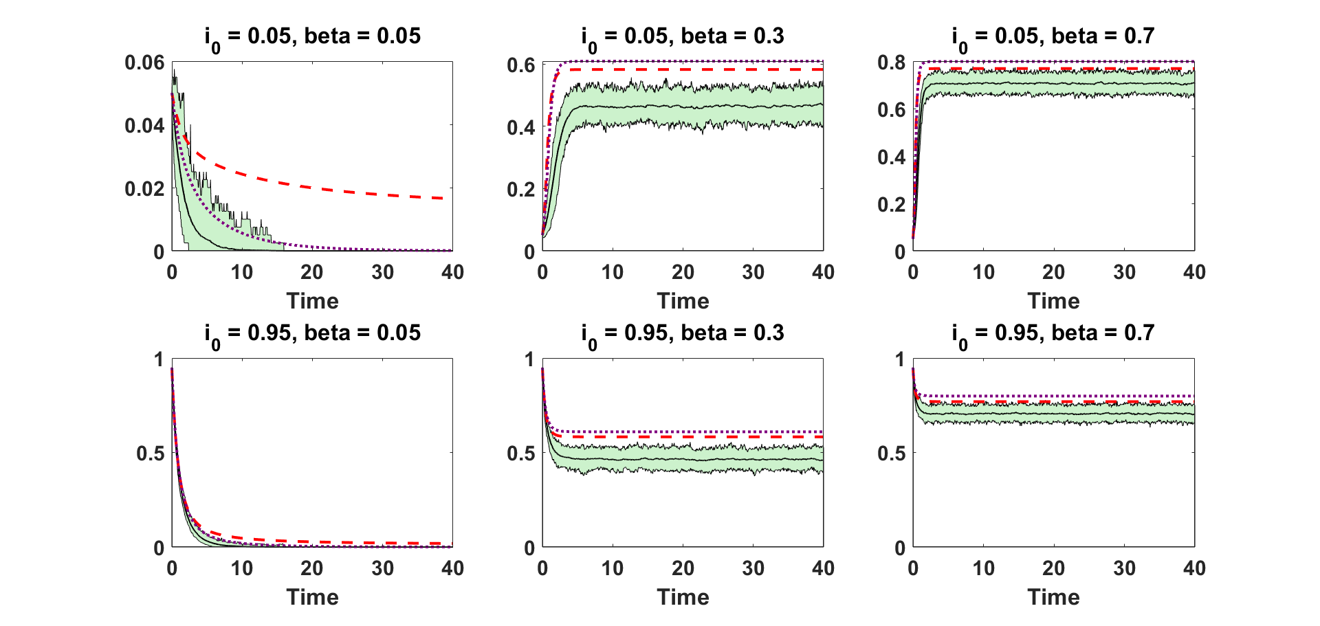
Figure 1: Infection function $\displaystyle f(x)=\mathrm{arctan}(x)$. Purple dots: mean field approximation from (8)–(9). Red dashed line: mean field approximation from (22)–(23). Black solid line: mean of the individual-level stochastic model.

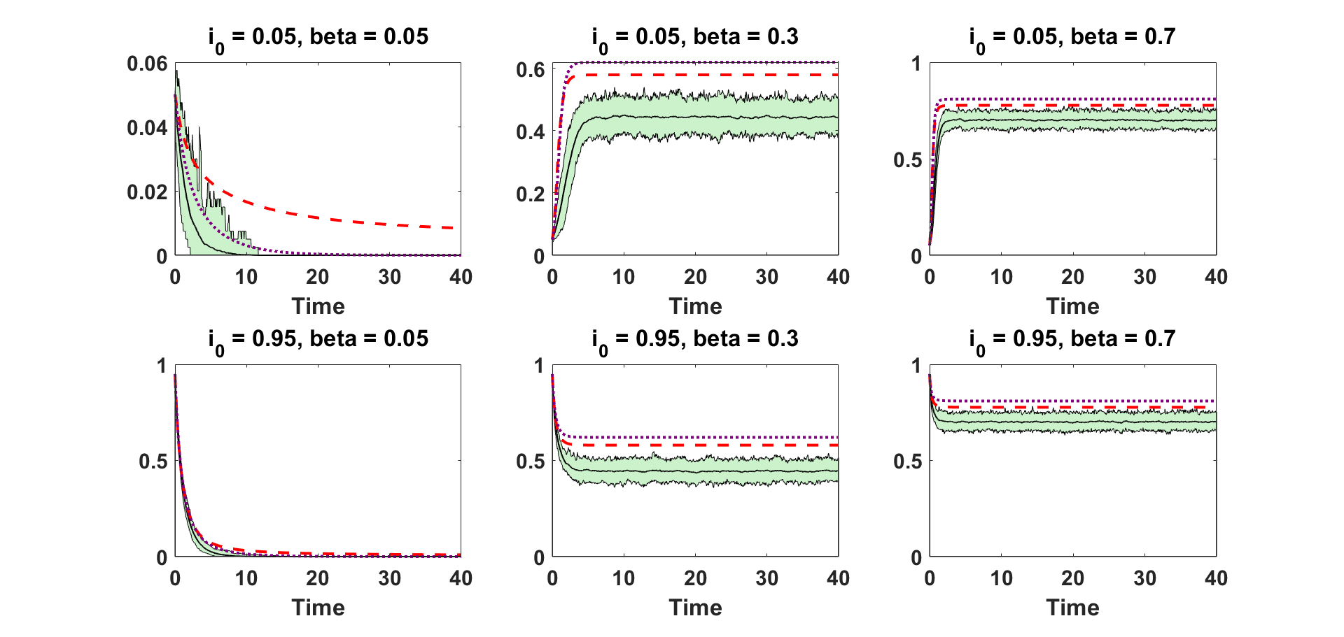
Figure 2: Infection function $\displaystyle f(x)=\log(1+x)$. Purple dots: mean field approximation from (8)–(9). Red dashed line: mean field approximation from (22)–(23). Black solid line: mean of the individual-level stochastic model.

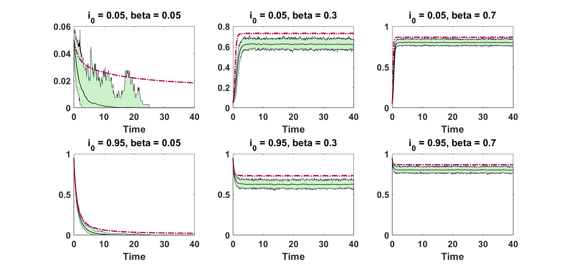
Figure 3: Infection function $\displaystyle f(x)=\min\{3,x\}$. Purple dots: mean field approximation from (8)–(9). Red dashed line: mean field approximation from (22)–(23). Black solid line: mean of the individual-level stochastic model.

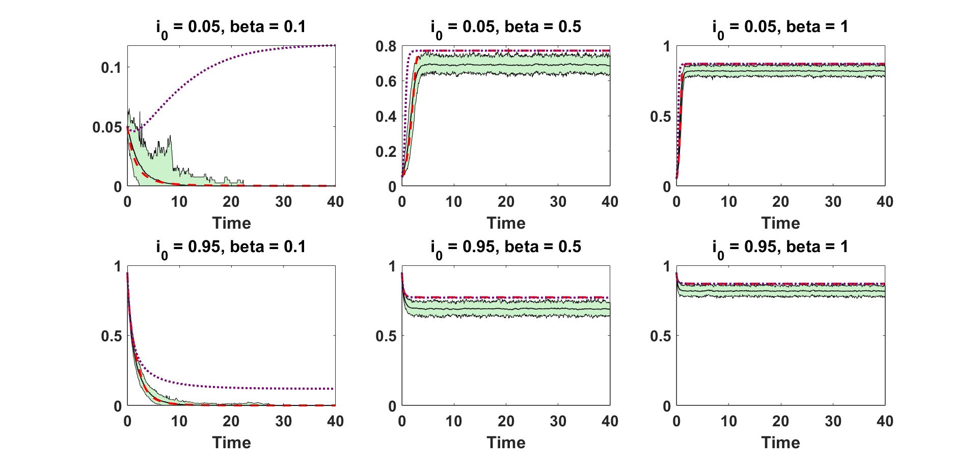
Figure 4: Collective contagion partitioned model. Purple dots: mean field approximation from (8)–(9). Red dashed line: mean field approximation from (22)–(23). Black solid line: mean of the individual-level stochastic model.

Figure 5: Infection function $\displaystyle 2\log(1+x)$ (left) and $\displaystyle\mathrm{arctan}$ (right). Horizontal axis is infection strength, $\displaystyle\beta$. Vertical axis is the proportion of infected individuals at time $\displaystyle T=200$ for the two mean field approximations, (22)–(23) (red dots) and (8)–(9) (black circles), and for the individual-level stochastic model (blue crosses), averaged over $\displaystyle 10$ runs. The spectral bounds on $\displaystyle\beta$ from (15) and (24) relating to the two mean field approximations, are shown respectively as a solid green vertical line (below which the red dots must be $\displaystyle 0$) and a dashed green vertical line (below which the black circles must be $\displaystyle 0$).

7.3 Collective contagion model: sensitivity to the initial condition

An interesting working assumption is that only hyperedges of size three or greater are present, and hence there are no pairwise interactions. This circumstance may arise, for example, if we restrict attention to a workplace or school environment. Here we look how this assumption may impact the predictive performance of the two mean field models, in the case of a collective contagion model. We used the same infection rate functions as in Figure 4. In Figures 6, 7, and 8, we show, for both mean field models and the exact stochastic model, the proportion of infected individuals at time $\displaystyle T=100$ averaged over $\displaystyle 5$ runs, as a function of the initial proportion $\displaystyle i_{0}$ of infected individuals. We observe that the mean field model given by (8)–(9) remains relatively stable, while the behaviour of the mean field model given by (22)–(23) appears to be sensitive to the initial condition $\displaystyle i_{0}$, its predictive performance degrading if $\displaystyle i_{0}$ is small (e.g., red dots in Figure 6). This sensitivity can be understood intuitively by recalling that the model in (8)–(9) is expressed as a continuous function of $\displaystyle P\in\mathbb{R}^{n}$, while the model in (22)–(23) is expressed in terms of step functions of the form $\displaystyle\mathbbm{1}(\sum_{i}p_{i}\mathcal{I}_{ih}\leq c_{1})$; the later are not continuous functions of $\displaystyle P$ and are more sensitive to small perturbations of the initial condition. Furthermore, for initial value $\displaystyle P(0)=(i_{0})_{i=1}^{n}$ sufficiently small that the threshold conditions of the above step functions are not satisfied, the infection rate expressed by (22)–(23) will remain $\displaystyle 0$, while the infection may start to spread according to the other models, thus yielding an underestimate of the propagation of the virus in the population.

We note that if the number of hyperedges is relatively low compared with the number of nodes (as in Figure 8), then the exact model will not propagate, in which case the mean field model given by (22)–(23) will give a better prediction. However, we see that both mean field models fail to accurately predict the behaviour of the model for sufficiently large initial condition $\displaystyle i_{0}$.

Figure 6: Proportion on infected individuals at time $\displaystyle T=100$ for the two mean field approximation models (red dots for (22)–(23) and black circles for (8)–(9)) and the individual-level stochastic model (blue crosses). Using $\displaystyle 200$ hyperedges of size $\displaystyle 3$, $\displaystyle 100$ hyperedges of size $\displaystyle 4$, $\displaystyle 50$ hyperedges of size $\displaystyle 5$ for $\displaystyle 400$ nodes.

Figure 7: Proportion on infected individuals at time $\displaystyle T=100$ for the two mean field approximation models (red dots for (22)–(23) and black circles for (8)–(9)) and the individual-level stochastic model (blue crosses). Using $\displaystyle 200$ hyperedges of size $\displaystyle 4$, $\displaystyle 100$ hyperedges of size $\displaystyle 5$ for $\displaystyle 400$ nodes.

Figure 8: Proportion on infected individuals at time $\displaystyle T=100$ for the two mean field approximation models (red dots for (22)–(23) and black circles for (8)–(9)) and the individual-level stochastic model (blue crosses). Using $\displaystyle 100$ hyperedges of size $\displaystyle 4$, $\displaystyle 50$ hyperedges of size $\displaystyle 5$ for $\displaystyle 400$ nodes.

8 Multi-type Model

In the above results, we assumed for simplicity that a fixed infection function $\displaystyle f$ applies for all hyperedges. The results, however, readily extend to a multi-type partition model, where the infection rate function may depend on the category and size of the hyperedge. As we discussed in section 2, the categories of hyperedge may correspond to locations, such as households, schools, offices, shops and public transport vehicles, and hyperedge size may have an impact on transmission if individuals are attempting to mutually distance. We will therefore explain how the main results change when we extend the infection rate model. Let us partition the hyperedges of the hypergraph into $\displaystyle S$ disjoint families $\displaystyle\{\mathcal{F}_{s}\}_{s=1}^{S}$, such that to each family $\displaystyle\mathcal{F}_{s}$ corresponds an infection function $\displaystyle f_{s}$. For each $\displaystyle s\in\{1,2,\dots,S\}$ we may further partition the hyperedges in $\displaystyle\mathcal{F}_{s}$ into disjoint categories $\displaystyle\mathcal{C}_{2}^{(s)},\dots,\mathcal{C}_{K_{s}}^{(s)}$, where a hyperedge $\displaystyle h\in\mathcal{F}_{s}$ belongs to $\displaystyle\mathcal{C}_{k}^{(s)}$ if and only if $\displaystyle|h|=k$. The infection rate model (4) may then be extended to

(26) $$\lambda_{i}(X(t))=\beta\,\sum_{s=1}^{S}\sum_{k=2}^{K_{s}}\sum_{h\in\mathcal{C}_{k}^{(s)}}{\mathcal{I}}_{ih}^{(s),(k)}\,f_{s}(\sum_{j=1}^{n}{\mathcal{I}}_{jh}^{(s),(k)}X_{j}),$$

where $\displaystyle\mathcal{I}^{(s),(k)}$ is the incidence matrix inducing the subhypergraph spanned by the hyperedges of $\displaystyle\mathcal{C}_{k}^{(s)}\subset\mathcal{F}_{s}$, i.e., $\displaystyle\mathcal{I}^{(s),(k)}_{ih}=1$ if $\displaystyle h\in\mathcal{C}_{k}^{(s)}\subset\mathcal{F}_{s}$ and $\displaystyle i\in h$, and $\displaystyle\mathcal{I}^{(s),(k)}_{ih}=0$ otherwise. We then have the following generalization of the ODE system in (8)–(9)

(27) $$\frac{dP(t)}{dt}=g(P(t)),$$

where $\displaystyle g\mathrel{\mathop{\ordinarycolon}}\mathbb{R}^{n}\to\mathbb{R}^{n}$ is defined by

(28) $$g_{i}(P(t))=\beta\sum_{s=1}^{S}\sum_{k=2}^{K_{s}}\sum_{h\in\mathcal{C}_{k}^{(s)}}\mathcal{I}^{(s),(k)}_{ih}(\sum_{l=1}^{k}f_{s}(l)\Psi(h,l))(1-p_{i}(t))-\delta p_{i}(t).$$

Define also $\displaystyle\mathcal{I}^{(s)}\mathrel{\mathop{\ordinarycolon}}=\sum_{k=2}^{K_{s}}\mathcal{I}^{(s),(k)}$ to be the incidence matrix inducing the subhypergraph spanned by the hyperedges in $\displaystyle\mathcal{F}_{s}$, and let $\displaystyle W^{(s)}\mathrel{\mathop{\ordinarycolon}}=\mathcal{I}^{(s)}(\mathcal{I}^{(s)})^{T}$, so that $\displaystyle W^{(s)}_{ij}$ records the number of hyperedges in $\displaystyle\mathcal{F}_{s}$ containing both $\displaystyle i$ and $\displaystyle j$. We then have the following results for the generalized partition model, which are extensions of Theorems 1, 2 and 3.

Theorem 1 (General condition for local asymptotic stability).

If

(29) $$\frac{\beta\,\lambda\left(\sum_{s=1}^{S}f_{s}(1)W^{(s)}\right)}{\delta}<1,$$

then $\displaystyle 0\in\mathbb{R}^{n}$ is a locally asymptotic stable equilibrium for (27)–(28).

Theorem 2 (Global asymptotic stability for a collective suppression model).

Suppose that $\displaystyle f_{s}$ is concave for all $\displaystyle s\in\{1,2,\dots,S\}$. If (29) holds, then $\displaystyle 0\in\mathbb{R}^{n}$ is globally asymptotically stable for (27)–(28).

Theorem 3 (Global asymptotic stability for a collective contagion model).

Suppose that for each $\displaystyle s\in\{1,2,\dots,S\}$, $\displaystyle f_{s}(x)\mathrel{\mathop{\ordinarycolon}}=c_{2,s}\mathbbm{1}(x\geq c_{1,s})$, where $\displaystyle c_{1,s}\geq 2$ and $\displaystyle c_{2,s}>0$. If

$$\frac{\beta\,\lambda\left(\sum_{s=1}^{S}\frac{c_{2,s}}{c_{1,s}}W^{(s)}\right)}{\delta}<1,$$

then $\displaystyle 0\in\mathbb{R}^{n}$ is globally asymptotically stable for (27)–(28).

9 Summary and Conclusions

Hypergraphs offer more flexibility and realism than pairwise, graph-based models and they are relevant to many spreading processes where members of a population form groups. In the pairwise setting, with linear infection rates, graph-based models have been widely studied, and spectral stability bounds derived [11, 13, 19, 24]. Spectral analysis for the hypergraph case was initially developed in [14], both for an exact individual-level stochastic model and a deterministic mean field approximation. In this work we focused on a more sophisticated mean field approximation that was proposed in [7] and requires a more detailed analysis. Although this ODE system produces real-valued trajectories, it has the unusual feature of evaluating the nonlinear infection rate function only at integer arguments. Intuitively, since the infection function is zero at the origin, this feature is likely to make the approximation more accurate than the version in [14] in the case of concave nonlinearity and small infection levels. This behaviour was observed in our computational tests (Figures 1–3 and Figure 5) and is backed by our theoretical analysis—in the concave case, this mean field model produces a locally asymptotically stable disease-free state under the same condition as the exact model (see Theorem 3 with $\displaystyle c_{f}=f(1)$ and Theorem 2). However, for other types of nonlinear infection rate, it is possible for the mean field model in [14] to give a better approximation (Figure 4). Hence the main conclusion from this work is that both mean field models can be analysed rigorously and both can provide useful information.

It is notable that the spectral conditions for decay of the disease level appearing in our results have the form

$$\frac{\beta\,c\,\lambda(W)}{\delta}<1,$$

for some constant $\displaystyle c$ that is determined by the type of nonlinear infection rate (with generalized versions in section 8). This expression separates out different aspects of the process in a natural manner and offers a means to inform mitigation strategies. The parameters $\displaystyle\beta$ and $\displaystyle\delta$ quantify the inherent infectiousness and recovery rate for the disease, respectively. The constant $\displaystyle c$ is affected by the way that the chance of a new infection depends on the number of infected people in a group. This could be controlled by changing behavioural patterns; for example, through face-covering or social distancing. The factor $\displaystyle\lambda(W)$, which summarizes the interaction structure, could be reduced by lockdown measures that restrict movement and therefore limit physical encounters. Hence, it would be of interest to calibrate a hypergraph model against real data and investigate the predictive power of these spectral bounds.

References

• [1] U. Alvarez-Rodriguez, F. Battiston, G. F. de Arruda, Y. Moreno, M. Perc, and V. Latora, Evolutionary dynamics of higher-order interactions in social networks, Nat. Hum. Behav., (2021).
• [2] F. Battiston, G. Cencetti, I. Iacopini, V. Latora, M. Lucas, A. Patania, J.-G. Young, and G. Petri, Networks beyond pairwise interactions: Structure and dynamics, Physics Reports, 874 (2020), pp. 1–92.
• [3] A. R. Benson, R. Abebe, M. T. Schaub, A. Jadbabaie, and J. Kleinberg, Simplicial closure and higher-order link prediction, Proceedings of the National Academy of Sciences, 115 (2018), pp. E11221–E11230.
• [4] A. R. Benson, D. F. Gleich, and J. Leskovec, Higher-order organization of complex networks, Science, 353 (2016), pp. 163–166.
• [5] A. Bodó, G. Katona, and P. Simon, SIS epidemic propagation on hypergraphs, Bulletin of Mathematical Biology, 78 (2016), pp. 713–735.
• [6] A. Bretto, Hypergraph Theory: An introduction, Springer, Berlin, 2013.
• [7] G. F. de Arruda, G. Petri, and Y. Moreno, Social contagion models on hypergraphs, Phys. Rev. Res., 2 (2020).
• [8] M.-A. de La Vega, G. Caleo, J. Audet, X. Qiu, R. A. Kozak, J. I. Brooks, S. Kern, A. Wolz, A. Sprecher, J. Greig, K. Lokuge, D. K. Kargbo, B. Kargbo, A. D. Caro, A. Grolla, D. Kobasa, J. E. Strong, G. Ippolito, M. V. Herp, and G. P. Kobinger, Ebola viral load at diagnosis associates with patient outcome and outbreak evolution, The Journal of Clinical Investigation, 125 (2015), pp. 4421–4428.
• [9] P. S. Dodds and D. J. Watts, A generalized model of social and biological contagion, Journal of Theoretical Biology, 232 (2005), pp. 587–604.
• [10] E. Estrada and J. A. Rodríguez-Velázquez, Subgraph centrality and clustering in complex hyper-networks, Physica A: Statistical Mechanics and its Applications, 364 (2006), pp. 581–594.
• [11] A. Ganesh, L. Massoulié, and D. Towsley, The effect of network topology on the spread of epidemics, Proceedings - IEEE INFOCOM, 2 (2005), pp. 1455–1466.
• [12] P. Hartman, On the stability in the large for systems of ordinary differential equations, Canadian Journal of Mathematics, 13 (1961), pp. 480–492.
• [13] H. A. Herrmann and J.-M. Schwartz, Why COVID-19 models should incorporate the network of social interactions, Physical Biology, 17, p. 065008.
• [14] D. J. Higham and H.-L. de Kergorlay, Epidemics on hypergraphs: Spectral thresholds for extinction, Proceedings of the Royal Society, Series A, 477 (2021).
• [15] I. Iacoponi, G. Petri, A. Barrat, and V. Latora, Simplicial models of social contagion, Nature Communications, 10 (2019).
• [16] I. Kiss, J. C. Miller, and P. L. Simon, Mathematics of Epidemics on Networks: From Exact to Approximate Models, Springer, Berlin, 2017.
• [17] A. Koriat, S. Adiv-Mashinsky, M. Undorf, and N. Schwarz, The prototypical majority effect under social influence, Personality and Social Psychology Bulletin, 44 (2018), pp. 670–683.
• [18] N. W. Landry and J. G. Restrepo, The effect of heterogeneity on hypergraph contagion models, Chaos, 30 (2020).
• [19] P. V. Mieghem, J. Omic, and R. Kooij, Virus spread in networks, IEEE Transactions on Networking, 17 (2009).
• [20] M. Petrovitch, Sur une manière d’étendre le théorème de la moyenne aux équations différentielles de premier ordre, Mathematische Annalen, 54 (1901), pp. 417–436.
• [21] J. J. Torres and G. Bianconi, Simplicial complexes: higher-order spectral dimension and dynamics, Journal of Physics: Complexity, 1 (2020), p. 015002.
• [22] F. Verhulst, Nonlinear Differential Equations and Dynamical Systems, Springer-Verlag, Berlin, 1990.
• [23] D. Wang, Y. Zhao, J. Luo, and H. Leng, Simplicial SIRS epidemic models with nonlinear incidence rates, Chaos: An Interdisciplinary Journal of Nonlinear Science, 31 (2021), p. 053112.
• [24] Y. Wang, D. Chakrabarti, C. Wang, and C. Faloutsos, Epidemic spreading in real networks: an eigenvalue point of view, Proceedings 22nd International Symposium on Reliable Distributed Systems, (2003).