Probing the $hc\bar{c}$ coupling at a Future Circular Collider
in the electron-hadron mode

Abstract

We study the production of a neutral Higgs boson at a Future Circular Collider in the electron-hadron mode (FCC-eh) through the leading process $e^{-}p\to\nu_{e}hq$ assuming the decay channel $h\to c\bar{c}$, where $h$ is the Standard Model (SM)-like state discovered at the Large Hadron Collider (LHC). This process is studied in the context of a 2-Higgs Doublet Model Type III (2HDM-III) embedding a four-zero texture in the Yukawa matrices and a general Higgs potential, where both Higgs doublets are coupled with up- and down-type fermions. Flavour Changing Neutral Currents (FCNCs) are well controlled by this approach through the adoption of a suitable texture once flavour physics constraints are taken in account. Considering the parameter space where the signal is enhanced and in agreement with both experimental data and theoretical conditions, we analyse the aforementioned signal by taking into account the most important SM backgrounds, separating $c$-jets from light-flavour and gluon ones as well as $b$-jets by means of efficient flavour tagging. We find that the $hc\bar{c}$ coupling strength can be accessed with good significance after a luminosity of $1$ ab^-1 for a 50 TeV proton beam and a 60 GeV electron one, the latter with a 80% (longitudinal) polarisation.

I Introduction

Since the July 2012 discovery of a Higgs boson, $h$, with properties very consistent with those predicted by the Standard Model (SM), at the Large Hadron Collider (LHC), by the ATLAS and CMS experiments, spontaneous Electro-Weak Symmetry Breaking (EWSB) resting on a minimal Higgs mechanism is apparently well established. While a mass of 125 GeV is not really an indication for the SM construct being the one responsible for these LHC signals, as $m_{h}$ is a free parameter in it, the fact that production and decay rates involving couplings to $W^{\pm}$ and $Z$ bosons as well as $t,b,\tau$ and $\mu$ fermions have been measured and are compatible with the SM genuine predictions (once $m_{h}$ is measured) is a strong sign in flavour of such a minimal Higgs construct.

However, a notable absence in the list of the SM-like Higgs couplings so far measured is the one involving the $hc\bar{c}$ vertex, which is presently unconstrained. The reason is that corresponding signals at the LHC are masked by an enormous QCD background. In fact, not even the ability to tag $c$-jets, on a similar footing with what has successfully been done for $b$-jets, is sufficient to enable a measurement of the Yukawa coupling to $c$-(anti)quarks at a level comparable to the case of $b$-ones, as the displaced vertex associated to semi-leptonic $c$-meson decays is much closer to the interaction point (where the gluon and light flavour jet backgrounds originates) than the one stemming from the corresponding $b$-meson transitions. Another drawback is that the strength of the $hc\bar{c}$ vertex in the SM is much smaller than that of the $hb\bar{b}$ vertex, as they scale with the fermion mass, which in turn means that the Branching Ratios (BRs) for $h\to c\bar{c}$ is $(m_{c}/m_{b})^{2}$ times smaller than BR($h\to b\bar{b}$), see, e.g., Ref. Moretti and Stirling (1995). On the other hand, the precise evaluation of decay width $h\to c\bar{c}$ has been studied recently at next-to-next-to-leading order QCD (including the flavour-singlet contribution) and the next-to-leading order electroweak Li et al. (2021).

However, there exist extensions of the SM in which the Higgs sector is enlarged by additional (pseudo)scalar multiplets (singlets, doublets, triplets, etc.), where the $h\to c\bar{c}$ rate can be increased substantially. Herein, owing to the fact that the SM-like Higgs discovered at the LHC has a clear doublet nature, we focus on the simplest extension of the SM involving such Higgs multiplet, the so-called 2-Higgs Doublet Model (2HDM). The latter comes in several guises, known as Type I, II, III (or Y) and IV (or X), wherein Flavour Changing Neutral Currents (FCNCs) mediated by (pseudo)scalars can be eliminated under discrete symmetries Branco et al. (2012); Barger et al. (1990); Grossman (1994); Aoki et al. (2009); Gunion et al. (2000); Donoghue and Li (1979); Barnett et al. (1984), entirely if the latter are exact or sufficiently to comply with experimental limits if they are softly broken. In fact, another, very interesting kind of 2HDM is the one where FCNCs can be controlled by a particular texture in the Yukawa matrices Fritzsch and Xing (2003). In particular, in previous papers, we have implemented a four-zero texture, in a scenario which we have called 2HDM Type III (2HDM-III) Diaz-Cruz et al. (2009). This model has a phenomenology that is very rich, which we studied at colliders in various instances Hernández-Sánchez et al. (2017); Hernandez-Sanchez et al. (2012), and some very interesting aspects, like flavour-violating quarks decays, which can be enhanced for neutral Higgs bosons with intermediate mass (i.e., below the top quark mass). In particular, we have studied the signal $\phi_{i}^{0}\to s\bar{b}+h.c.$ ($\phi_{i}^{0}=h,\,H$) Hernandez-Sanchez et al. (2015); Das et al. (2016). Furthermore, in this model, the parameter space can avoid the current experimental constraints from flavour and Higgs physics and a light charged Higgs boson is allowed Hernandez-Sanchez et al. (2013), so that the decay $H^{-}\to b\bar{c}$ is enhanced and its BR can be dominant Akeroyd et al. (2017, 2012).

In fact, the 2HDM-III is also an ideal candidate in providing enhanced $h\to c\bar{c}$ rates, as the Yukawa texture parameters that affect the aforementioned $H^{\pm}$ signatures also enter the $h\to b\bar{b}$ and $h\to c\bar{c}$ ones. In particular, it is always possible to maintain the Yukawa coupling to the $b$-(anti)quark in the range currently measured at the LHC, and indeed the one foreseen by the end of the High Luminosity LHC (HL-LHC) era Gianotti et al. (2005); Apollinari et al. (2017), while enhancing the $h\to c\bar{c}$ one. It is the purpose of this paper to study the scope of the electron-proton Future Circular Collider (FCC-eh), with a Center-of-Mass (CM) energy of 3.5 TeV Kuze (2018); Britzger and Klein (2018); Abada et al. (2019a). This configuration is obtained by the collisions of a 50 TeV proton beam coming from the FCC-hh Abada et al. (2019b) and a 60 GeV electron beam from an external linear accelerator (Electron Recovery Linac (ERL)) tangential to the FCC main tunnel Abada et al. (2019a) and offers good prospects as a Higgs boson factory, as herein one could elucidate the nature of the couplings of generic Higgs bosons to most fermions, especially the $h\to b\bar{b}$ one, which remains difficult to establish with high precision at both the LHC and the HL-LHC because of the overwhelming QCD background . Given these encouraging results for the $hb\bar{b}$ vertex, we specifically analyse here the prospects of also establishing the $hc\bar{c}$ one.

Our work is organised as follows. In the next section we describe briefly the 2HDM-III, specifically, its Yukawa structure. Then in the following one we discuss the theoretical and experimental constraints applying to it and select some benchmark scenarios for numerical analysis. In section IV we give our results whereas in section V we finally summarise.

II The Higgs sector of the 2HDM-III

The 2HDM-III is described by two scalar Higgs doublets $\Phi_{i}=(\phi_{i}^{-},\,\phi_{i}^{0*})$ ($i=1$, 2), with hypercharge $+1$, which can couple to all fermions. FCNCs are controlled by a specific four-zero texture in the Yukawa matrices, the latter being an effective flavour theory of the Yukawa sector. Therefore, a discrete symmetry is not necessary in this approach, so that the $SU(2)_{L}\times U(1)_{Y}$ invariant scalar potential in its general form can be considered, which is given by Haber and Hempfling (1993); Gunion and Haber (2003); Dubinin and Semenov (2003); Gunion and Haber (2005):

$$V(\Phi_{1},\Phi_{2}) = \mu_{1}^{2}(\Phi_{1}^{\dagger}\Phi_{1})+\mu_{2}^{2}(\Phi_{2}^{\dagger}\Phi_{2})-\Big{(}\mu_{12}^{2}(\Phi_{1}^{\dagger}\Phi_{2}+h.c.)\Big{)}$$ (1)

$$+\frac{1}{2}\lambda_{1}(\Phi_{1}^{\dagger}\Phi_{1})^{2}+\frac{1}{2}\lambda_{2}(\Phi_{2}^{\dagger}\Phi_{2})^{2}+\lambda_{3}(\Phi_{1}^{\dagger}\Phi_{1})(\Phi_{2}^{\dagger}\Phi_{2})+\lambda_{4}(\Phi_{1}^{\dagger}\Phi_{2})(\Phi_{2}^{\dagger}\Phi_{1})$$

$$+\left(\frac{1}{2}\lambda_{5}(\Phi_{1}^{\dagger}\Phi_{2})^{2}+\lambda_{6}(\Phi_{1}^{\dagger}\Phi_{1})(\Phi_{1}^{\dagger}\Phi_{2})+\lambda_{7}(\Phi_{2}^{\dagger}\Phi_{2})(\Phi_{1}^{\dagger}\Phi_{2})+h.c.\right),$$

wherein, for simplicity, we suppose that all parameters are real as so are the Vacuum Expectation Values (VEVs) of the Higgs fields. Besides, notice that, when a discrete symmetry is implemented in the model, the $\lambda_{6,7}$ terms are absent. However, in our model, the latter can be kept in the Higgs potential when the four-zero texture is implemented in the Yukawa matrices. This is rather interesting, as we have shown that these parameters ($\lambda_{6,7}$) can be relevant in one-loop processes but do not contribute to EW parameter $\rho=m_{W}^{2}/m_{Z}^{2}\cos_{W}^{2}$ Cordero-Cid et al. (2014). However, the ordinary custodial symmetry Branco et al. (2012); Gunion et al. (2000)(twisted custodial symmetry Gerard and Herquet (2007)) associated to the $\rho$ parameter is broken when the difference $m_{H^{\pm}}-m_{A}$($m_{H^{\pm}}-m_{H}$) is sizeable, being $H^{\pm}$ the charged Higgs boson and $A(H)$ the heavy CP-odd(even) one belonging to this construct, in addition to the aforementioned SM-like $h$ state. Reasonable models with such an extended Higgs sector are those for which $\rho\approx 1$ when radiative corrections are included Toussaint (1978); Bertolini (1986); Hollik (1986); Gunion and Turski (1989); Gunion et al. (2000); Gunion and Haber (2003); Gerard and Herquet (2007); de Visscher et al. (2009) or, more in general, those in good agreement with the experimental constraints from the oblique parameters $S$, $T$ and $U$ Haller et al. (2018); Kanemura et al. (2011), part of the so-called EW Precision Observables (EWPOs) Zyla et al. (2020). The described Higgs bosons spectrum emerges after EWSB, which provide mass to the $W^{\pm}$ and $Z$ bosons, thus releasing five physical Higgs fields: two CP-even neutral states $h,H$ (with $m_{h}<m_{H}$), one CP-odd neutral state $A$ plus two charged Higgs bosons $H^{\pm}$. Furthermore, one also has the mixing angle $\alpha$, that relates the two CP-even neutral bosons $(h,H)$ and $\beta$ (being $\tan\beta$ the ratio of VEVs of the two Higgs doublets). The masses of these Higgs fields and these two angles are the inputs parameters chosen here to describe the scalar potential.

About the Yukawa sector of our model, this is defined by Hernandez-Sanchez et al. (2013):

$${\cal{L}}_{Y}=-\left(Y_{1}^{u}\bar{Q}_{L}\tilde{\Phi}_{1}u_{R}+Y_{2}^{u}\bar{Q}_{L}\tilde{\Phi}_{2}u_{R}+Y_{1}^{d}\bar{Q}_{L}\Phi_{1}d_{R}+Y_{2}^{d}\bar{Q}_{L}\Phi_{2}d_{R}+Y_{1}^{l}\bar{L}_{L}\tilde{\Phi}_{1}l_{R}+Y_{2}^{l}\bar{L}_{L}\tilde{\Phi}_{2}l_{R}\right),$$ (2)

being $\tilde{\Phi}_{i}=i\sigma_{2}\Phi_{i}^{*}$ ($i=1,2$) and where both Higgs doublets are coupled with up- and down-type fermions. Following the procedure of Refs. Félix-Beltrán et al. (2015); Hernandez-Sanchez et al. (2013), after EWSB, the fermion mass matrices are:

$$M_{f}=\frac{1}{\sqrt{2}}(v_{1}Y_{1}^{f}+v_{2}Y_{2}^{f})\ \ \ (f=u,d,\ell),$$ (3)

where the Yukawa matrices $Y_{1,2}^{f}$ have the four-zero texture form and are Hermitian. Considering the diagonalisation of the fermion mass matrices through $\bar{M}_{f}=V_{fL}^{\dagger}M_{f}V_{fL}$, we have $\tilde{Y}_{n}^{f}=V_{fL}^{\dagger}Y_{n}^{f}V_{fL}$, then one can get a good approximation for the rotated matrix $\tilde{Y}_{n}^{f}$ as follows Hernandez-Sanchez et al. (2013):

$$\Big{(}\tilde{Y}_{n}^{f}\Big{)}_{ij}=\frac{\sqrt{m_{i}^{f}m_{j}^{f}}}{v}(\tilde{\chi}^{f})_{ij}=\frac{\sqrt{m_{i}^{f}m_{j}^{f}}}{v}\chi_{ij}^{f}e^{\theta_{ij}^{f}},$$ (4)

where the $\chi$s are dimensionless and constrained by flavour physics experimental data, which will be discussed in the following section. Then, one can obtain the generic Lagrangian of the Yukawa sector, which gives the interactions of physical (pseudo)scalars fields with fermions, as:

$${\cal{L}}^{\bar{f}_{i}f_{j}\phi} = -\left\{\frac{\sqrt{2}}{v}\bar{u}_{i}\big{(}m_{d_{j}}X_{ij}P_{R}+m_{u_{i}}Y_{ij}P_{L}\big{)}d_{j}H^{+}+\frac{\sqrt{2}m_{l_{j}}}{v}Z_{ij}\bar{\nu}_{L}l_{R}H^{+}+h.c.\right\}$$ (5)

$$-\frac{1}{v}\left\{\bar{f}_{i}m_{f_{j}}h_{ij}^{f}f_{j}h^{0}-i\bar{f}_{i}m_{f_{i}}A_{ij}^{f}f_{j}\gamma_{5}A^{0}\right\},$$

where $X_{ij}$, $Y_{ij}$, $Z_{ij}$, $A_{ij}$ are given in Hernandez-Sanchez et al. (2013). For our study it is sufficient to consider the functions $h_{ij}^{f}$, which are given by:

$$h_{ij}^{u} = \varepsilon_{h}^{u}\delta_{ij}-\frac{\big{(}\varepsilon_{H}^{u}+Y\varepsilon_{h}^{u}\big{)}}{\sqrt{2}f(Y)}\sqrt{\frac{m_{u_{j}}}{m_{u_{i}}}}\chi_{ij}^{u},$$ (6)

$$h_{ij}^{d} = \varepsilon_{h}^{d}\delta_{ij}+\frac{\big{(}\varepsilon_{H}^{d}-X\varepsilon_{h}^{d}\big{)}}{\sqrt{2}f(X)}\sqrt{\frac{m_{d_{j}}}{m_{d_{i}}}}\chi_{ij}^{d},$$ (7)

wherein the parameters $X$, $Y$, $\varepsilon_{h,H}^{u,d}$ are given in Table 1, where it is made clear that our 2HDM-III construct with a four-zero Yukawa texture can be related to the ordinary Yukawa types known as Type I, II and Y (or flipped) by choosing appropriately these parameters.

2HDM-III	$X$	$Y$	$\varepsilon_{h}^{u}$	$\varepsilon_{h}^{d}$
2HDM-I	$-\cot\beta$	$\cot\beta$	$\cos\alpha/\sin\beta$	$\cos\alpha/\sin\beta$
2HDM-II	$\tan\beta$	$\cot\beta$	$\cos\alpha/\sin\beta$	$-\sin\alpha/\cos\beta$
2HDM-Y (flipped)	$\tan\beta$	$\cot\beta$	$\cos\alpha/\sin\beta$	$-\sin\alpha/\cos\beta$

Table 1: The parameters choices for $X$, $Y$ and $\varepsilon_{h}^{u,d}$ of the 2HDM-III needed to obtain the standard 2HDM Type I, II and Y (flipped), which happen when the $\chi$s are zero.

In general, the Higgs-fermion-fermion couplings are expressed as $g^{ff\phi}_{\rm 2HDM-III}=g^{ff\phi}_{\rm any}+\Delta g$, where $g^{ff\phi}_{\rm any}$ represents the $ff\phi$ coupling in any 2HDM with a discrete symmetry and $\Delta g$ is the contribution of the four-zero texture Hernandez-Sanchez et al. (2013).

III Constraints and Benchmark Scenarios

In previous works Diaz-Cruz et al. (2009); Félix-Beltrán et al. (2015); Hernandez-Sanchez et al. (2013); Cordero-Cid et al. (2015), we have constrained our model by considering EWPOs, flavour and Higgs physics constraints from experimental data as well as theoretical bounds (such as unitarityCasalbuoni et al. (1986); Ginzburg and Ivanov (2005), vacuum stability Ferreira et al. (2004); Ivanov (2008) and perturbativity). Since the theoretical bounds and EWPO constraints have been analysed very recently Hernández-Sánchez et al. (2020), and these have not changed, we refer the reader to such a paper. In contrast, experimental constraints evolve continuously so here we have re-evaluated them in the light of the very latest results. Specifically, the parameter space of the model was constrained by flavour physics measurements, through the experimental data bounds from leptonic and semileptonic meson decays, the inclusive decay $B\to X_{s}\gamma$ , the $B_{0}-B_{0}$ and $K_{0}-K_{0}$ mixing as well as the process $B_{s}\to\mu^{+}\mu^{-}$ Hernandez-Sanchez et al. (2013); Crivellin et al. (2013). We have then used HiggsBounds Zyla et al. (2020); Aad et al. (2020a) and HiggsSignals Aad et al. (2016); Sirunyan et al. (2019a) to place bounds over the masses and couplings of neutral Sirunyan et al. (2020); Khachatryan et al. (2016) and charged Higgs bosons Abbiendi et al. (2013); Abbott et al. (1999); Abulencia et al. (2006); Abazov et al. (2009); Sirunyan et al. (2018a, 2019b), so as to make sure that the parameter space of the 2HDM-III considered here is consistent with any Higgs boson searches and measurements conducted at the LHC and previous colliders. In particular, using LHC measurements of the SM-like Higgs boson in the decays $h\to\gamma\gamma$ and $\gamma Z$ Aaboud et al. (2018a, b); Aad et al. (2020b); Aaboud et al. (2017); Sirunyan et al. (2019c, 2018b), we made sure that the Yukawa texture involving the couplings of the charged Higgs boson with fermions in the loops of these processes is in agreement with data. Specifically, in the permitted region of parameter space of our model, rather low masses for the charged Higgs bosons are allowed Cordero-Cid et al. (2014, 2015); Hernández-Sánchez et al. (2020); Flores-Sánchez et al. (2019).

As intimated, in this study, the scalar field $h$ is the SM-like Higgs boson, hence, $m_{h}=125$ GeV. Furthermore, we choose the following parameter space: $m_{A}=150$ GeV, 125 GeV $<m_{H}<$ 200 GeV, 100 GeV $<m_{H^{\pm}}<170$ GeV and $\cos(\beta-\alpha)\approx 0.1$, with $0.014\leq S\leq 0.026$ and $-0.02\leq T\leq 0.028$ and tensioned these against the measured values $S=-0.01\pm 0.07$ and $T=0.04\pm 0.06$ (fixing $U=0$) taken from Workman and Others (2022), being all this parameter space consistent with the aforementioned theoretical conditions and experimental data. Then, we select some sets of free parameters $\chi$’s which will represent our benchmark scenarios for each of the discussed 2HDM-III realisations (or incarnations). Explicitly, these benchmark scenarios are shown in Table 2.

Scenario	$\cos(\beta-\alpha)$	$\chi^{u}_{\{22,23,33\}}$	$\chi^{d}_{\{22,23,33\}}$	$\chi^{l}_{\{22,23,33\}}$
Ia	0.1	$\{1,0.1,1.4\}$	$\{1.8,0.1,1.2\}$	$\{-0.4,0.1,1\}$
IIa	0.1	$\{1,-0.53,1.4\}$	$\{1.8,0.2,1.3\}$	$\{-0-4,0.1,1\}$
Y	0.1	$\{1,-0.53,1.4\}$	$\{1.8,0.2,1.3\}$	$\{-0-4,0.1,1\}$

Table 2: Values for free parameters which define our benchmark scenarios, all being consistent with current theoretical and experimental bounds.

We have characterised these benchmark scenarios in Figure 1, where we show the events rates for the aforementioned production and decay process over the $(X,Y)$ plane for case Ia, IIa and Y of Table 2. These events rates are realised at parton level, taking the efficiency of $c$-tagged jets as $\epsilon_{c}=0.24$ and assuming 1 ab^-1 of (integrated) luminosity. The coloured regions over the $(X,Y)$ plane shown herein are compliant with all aforementioned constraints while the white backgrounds correspond to regions ruled out. Furthermore, we have demanded that for all benchmark points the BR$(h\to b\bar{b})$ is in agreement with the latest experimental observations, which established as ratio of the measured value to the SM prediction the following one $\mu=1.04\pm 0.20$ Sopczak (2020); Aaboud et al. (2018c); Sirunyan et al. (2018c). Moreover, we have considered the most recent and stringent direct constraint for the Higgs-charm Yukawa coupling modifier $\kappa_{c}$ obtained by CMS and ATLAS Aad et al. (2022); CMS (2022), where $1.1<|\kappa_{c}|<5.5$ and this one is interpreted in the $\kappa$-framework Andersen et al. (2013); de Florian et al. (2016). These last constraints are responsible for the absence of continuity across all allowed regions. This is due to the fact that the Yukawa couplings are strongly sensitive to the $X$ and $Y$ values, hence the BR$(h\to b\bar{b})$ is too, as well as BR$(h\to c\bar{c})$. For example, for the Ia scenario, over the region with $2<X<5$, the BR$(h\to b\bar{b})$ is above the mentioned experimental bounds but, if $Y$ grows larger, $h\to c\bar{c}$ starts to be relevant and the BR$(h\to b\bar{b})$ decreases until acceptable values. In contrast, in the region $0<X<1$, the channel $h\to b\bar{b}$ is generally inconsistent with experimental data unless $Y$ is small, so that the $h\to c\bar{c}$ decay rate is small too and the BR$(h\to b\bar{b})$ is within the allowed limits from the experimental data connected at the CERN machine.

The discussed event rates are calculated via the formula $\sigma(ep\to\nu_{e}hj)~{}\times$ BR$(h\to c\bar{c})\times$ 1 ab${}^{-1}~{}\times\epsilon_{c}^{2}$ (as mentioned, we take $\epsilon_{c}=0.24$ as an approximation of the efficiency of a standard $c$-tagging algorithm suitable for the FCC-eh environment U. Klein et al. (2014)). The cross sections and BRs have been calculated using CalcHEP 3.7.5 Belyaev et al. (2013), wherein the 2HDM-III has been implemented by ourselves. The proton beam is taken with $50$ TeV of energy ($E_{b}$), assuming CTEQ6L1 as Parton Distribution Functions (PDFs) Pumplin et al. (2002), while the electron beam is considered to be of $60$ GeV ($E_{e^{-}}$) with a (longitudinal) polarisation ($P_{L}^{\;e^{-}}$) of $-80\%$ Agostini et al. (2020). For each of these BPs we give herein the common cross section, the BRs into $b\bar{b}$, $c\bar{c}$, $s\bar{b}$ plus Charge Conjugate (C.C.) and $s\bar{s}$.

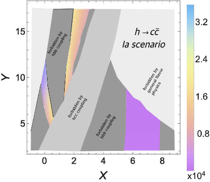
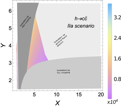
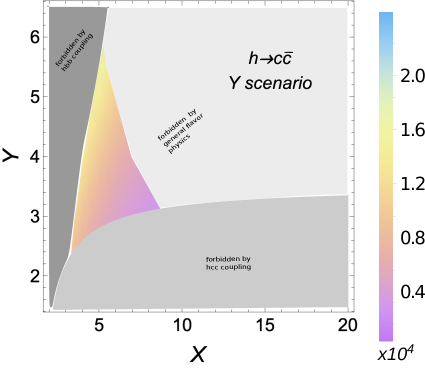
Figure 1: Event rates for each benchmark scenario over the $(X,Y)$ plane computed as $\sigma(ep\to\nu_{e}hj)\times{\rm BR}(h\to c\bar{c})\times\epsilon_{c}^{2}\times 1~{}{\rm ab}^{-1}$. Here, we have $E_{p}=50$ TeV and $E_{e^{-}}=60$ GeV (with $P_{L}^{\;e^{-}}=-80\%$).

Point	$X(Z)$	$Y$	BR$(\phi^{0}\to ab)$	$\sigma(e^{-}p\to e^{-}\phi^{0}q)$	Events (1 ab-1)
			BR$(h\to b\bar{b})=0.513$		$2\times 10^{5}$
Ia	0.5(0.5)	6.5	BR$(h\to c\bar{c})=0.484$		$2\times 10^{4}$
	$\mu=0.88$		BR$(h\to sb)=1.99\times 10^{-3}$	$0.875$ pb	$52$
	$\kappa_{c}=1.5$		BR$(h\to s\bar{s})=8.18\times 10^{-9}$		$0$
			BR$(h\to b\bar{b})=0.67$		$2\times 10^{5}$
IIa	1(1)	4	BR$(h\to c\bar{c})=0.23$	$0.958$ pb	$2\times 10^{4}$
	$\mu=1.16$		BR$(h\to sb)=0.093$		$1\times 10^{3}$
	$\kappa_{c}=2$		BR$(h\to s\bar{s})=2.87\times 10^{-3}$		$7$
			BR$(h\to b\bar{b})=0.498$		$2\times 10^{5}$
Y-min	5(-1/5)	5	BR$(h\to c\bar{c})=0.289$	$1.08$ pb	$2\times 10^{4}$
	$\mu=0.86$		BR$(h\to sb)=0.21$		$7\times 10^{3}$
	$\kappa_{c}=1.7$		BR$(h\to s\bar{s})=1.96\times 10^{-3}$		$5$

Table 3: Relevant cross sections, BRs and event rates (for the machine configuration given in the previous figure caption) for our scenarios Ia, IIa and Y, each mapped in terms of $X,Y$ and $Z$ values. We have included the allowed values for $\mu$ and $\kappa_{c}$ for each BPs. Here, we have included the following tagging efficiencies in the last column: $\epsilon_{b}=0.6$, $\epsilon_{c}=0.24$ and $\epsilon_{s}=0.05$ U. Klein et al. (2014).

As prospect of our work, for ee-colliders as ILC Aihara et al. (2019) ( CLIC et al. (2018)) machine the cross sections of Higgs production would be $\sigma(e^{+}e^{-}\to\nu_{e}\bar{\nu_{e}}h)\sim 220$ fb ($\sim 600$ fb) and the main cross section $\sigma(e^{-}p\to hj\nu_{e})\sim 190$ fb ($\sim 1000fb$) for electron proton-colliders LHeC (FCC-he), with center-of mass energy of $\sqrt{s}=1.3$TeV ( $\sqrt{s}=3.5$ TeV) . One can see, the cross sections are the same order of magnitude. Therefore, the studies of Higgs factories would be complement among ee-colliders and ep- colliders.

IV Numerical Analysis

The first step of our numerical analysis is to compare the production and decay rate of signal events to those of the various backgrounds, in presence of acceptance and selection cuts. The latter are implemented at the parton level as $p_{T}(q)>10$ GeV, $\Delta R(q,q)>0.3$ and $|\eta(q)|<7$, where $q$ represents any quark involved. For our Signal ($S$), we refer to the inclusive rates in Table 3. For the Background ($B$), final states of the type $E_{T}/~{}~{}~{}+3$ jet are considered. In order to not overload with information the forthcoming histograms, we consider the following five compounded contributions (wherein $j$ represents any jet except a $b$-one): $\nu 3j$ (it represents the set of $\nu_{e}jjj$, $\nu_{e}bjj$ and $\nu_{e}bbj$ final states), $\nu_{e}llj$ (for any configuration of charged leptons and quarks), $\nu_{e}tb$, $e3j$ (for $ejjj$, $ebjj$ and $ebbj$) and $ett$. In Table 4, one can see the corresponding cross sections at parton level for all these backgrounds as well as the corresponding event rates for the usual FCC-eh parameters.

Background	Cross section [pb]	Number of events
$\nu_{e}jjj$	172	$1.75\times 10^{8}$
$\nu_{e}bjj$	16.1	$1.61\times 10^{7}$
$\nu_{e}bbj$	1.8	$1.8\times 10^{6}$
$\sum\nu 3j$	189.9	$10^{8}$
$\nu_{e}llj$	3.09	$3.09\times 10^{6}$
$\nu_{e}tb$	12.47	$1.24\times 10^{7}$
$ejjj$	948	$9.48\times 10^{8}$
$ebjj$	17.8	$1.78\times 10^{7}$
$ebbj$	75.4	$75.4\times 10^{7}$
$\sum ejjj$	1040	$10^{9}$
$ett$	0.35	$3.5\times 10^{5}$

Table 4: Background cross sections and event rates at parton level after the following cuts: $p_{T}(q)>10$ GeV, $\Delta R(q,q)>0.3$ and $|\eta(q)|<7$ (assuming the usual FCC-eh parameters).

For the analysis at detector level, we proceed in the following way: we use PYTHIA8 Sjöstrand et al. (2015) as parton shower and hadronisation generator and Delphes de Favereau et al. (2014) as detector simulator. Delphes was run via a FCC-eh card provided in U. Klein et al. (2017). Finally, we employed MadAnalysis5 Conte et al. (2013) to construct histograms and implement the event selections.

In order to reconstruct the final state of interest, enriched by two $c$-jets, we need to worry about the presence of $b$-jets, as both $c$- and $b$-quarks will originate jets with displaced vertices: thus, just like there is a non-zero probability of $b$-jets being tagged as $c$-jets also the vice versa is possible. Furthermore, a value of $60\%$ for $\epsilon_{b}$ essentially means that some $b$-jets (precisely, 40% of them) could be tagged as either $c$-jet or lighter ones. In essence, it is not obvious what will be the number of true $c\bar{c}$ events in the complete di-jet sample (although this is all modelled by Delphes). However, in order to extract the $hc\bar{c}$ vertex strength, we can proceed as follows. To start with, the portion of $b\bar{b}$ events recognised as such, $N_{b}\approx\epsilon_{b}^{2}$, can be filtered out. Conversely, around $1-\epsilon_{b}^{2}$ of $b\bar{b}$ events would be accounted as light di-jets ones (including $c\bar{c}$ ones, that we do not separate out), which we label as $N_{b\to j}$. (In fact, the latter also includes a $\propto(1-\epsilon_{b})$ subleading contribution from mistagged $s\bar{b}$ + C.C. events.) This will add to the true number of events with only light jets, $N_{j}$, where $j=s$. Likewise, the portion of $c\bar{c}$ events recognised as such is $N_{c}=\epsilon_{c}^{2}$, which in turn implies that $1-\epsilon_{c}^{2}$ of these will appear as light jets, labelled as $N_{c\to j}$. These will also add to the $N_{j}$ rate alongside the $N_{b\to j}$ one. In order to perform an unbiased measurement of the Yukawa coupling $hc\bar{c}$ we can only rely on the $N_{c}$ sample. However, we can use the sample constituted by $N_{j}+N_{b\to j}+N_{c\to j}$ di-jet events, wherein it is not necessary to extract the fraction of $b$-jets appearing as $c$-jets, for validation purposes, to ensure that the two measurements are consistent with each other, so that, in the remainder of our analysis, we will consider the two cases in parallel.

Now, having defined two di-jet samples accounting for flavour (mis)tagging effects, in order to remove the contamination from backgrounds having kinematic configurations similar to the signals, irrespectively of the flavour composition, we proceed by enforcing the following sets of cuts. (Notice that the kinematics of any $h$ decay into di-jets is the same, given the much larger value of $m_{h}=125$ GeV with respect to any $m_{q}$ with $q=d,u,s,c$ and $b$.)

• We impose the following initial conditions for jets and leptons: $p_{T}(j)>10$ GeV, $p_{T}(l)>10$ GeV and $|\eta(j)|<6$. Once these requirements are combined with the described tagging procedure, we have events composed of missing (transverse) energy and three jets.

• From the left histogram of Figure 2, one can select the most relevant signature in terms of jet multiplicity, specifically, we select events with exactly two jets. In fact, the third jet typically comes directly from the primary vertex and is very forward, when not outside the detection zone (i.e., $|\eta(j_{3})|>6$), therefore it is not considered in our analysis. Furthermore, for any jet multiplicity $N[j]>3$, the signal yield is far too depleted to be of numerical interest. Another cut is over the missing (transverse) energy, as we take $E_{T}/~{}~{}~{}>30$ GeV (see the histogram on the right-hand side of Figure 2). Specifically, this cut is very strong against the $ejjj$ background, as it keeps only around $20\%$ of such events without penalising the signals excessively.

• The third set of cuts are imposed over the pseudorapidity and transverse momentum of each jet. To start with, we use $\eta$ ordering to tag the first or second jet (i.e., $|\eta(j_{1})|>|\eta(j_{2})|$). About pseudorapidity, we demand $\eta(j_{1})<-3.5$ and $\eta(j_{2})<-4$. These cuts are highly restrictive onto $ejjj$ and $\nu jjj$, keeping around of $8\%$ and $50\%$ of these events, respectively (see top histograms in Figure 3). Furthermore, the selections in jet transverse momentum are $p_{T}(j_{1})<90$ GeV, which has a strong impact on the $ejjj$ and $ett$ backgrounds, and $p_{T}(j_{2})>30$ GeV, which affects mainly the $\nu jjj$ and $\nu tb$ noises (see bottom histograms in Figure 3).

• We impose that $\Delta R(j_{1},j_{2})\equiv\sqrt{\Delta\phi(j_{1},j_{2})^{2}+\Delta\eta(j_{1},j_{2})^{2}}>1.6$. This cut enhances the signal above all backgrounds except $ejjj$: see Figure 4.

• Finally, we impose a selection on invariant mass for of the two jets, which are the candidates to reconstruct the SM-like Higgs boson mass. Specifically, this cut is $100$ GeV$<M(j_{1},j_{2})<125$ GeV: see Figure 5.

(Notice that we have illustrated the kinematics of the Ia incarnation of the 2HDM-III signal but we can confirm that results are extremely similar for the IIa and Y cases as well.)

The response of all signals and backgrounds to each of the above cuts is captured in Table 5. Here, the top value in each row represents the signal rate with no flavour being filtered, i.e., this is the effective di-jet final state defined above as $N_{j}+N_{b\to j}+N_{c\to j}$ while the bottom value is the estimated number of $N_{c}$ events made up by $c\bar{c}$ pairs recognised as such. It is clear that the kinematic selection is effective in significantly reducing all of the latter without greatly affecting all of the former. This is well exemplified by the values of the final $S$ versus $B$ rates, including the significances, defined as $\frac{S}{\sqrt{S+B}}$. The fact that the corresponding values are always well beyond 5, whichever flavour tagging, clearly indicates the discovery potential of both $h\to jj$ and $h\to c\bar{c}$ events at the FCC-eh with a confidence level against the possibility of a background fluctuation far higher than at any hadron collider foreseen at CERN, i.e., a HL-LHC and FCC-hh Apollinari et al. (2017); Abada et al. (2019c), and comparable to that of the FCC-ee Abada et al. (2019d), a future $e^{+}e^{-}$ collider therein.

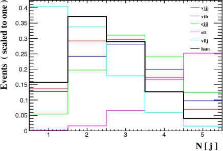
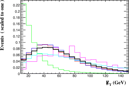
Figure 2: Left) Jet multiplicity (whichever their flavour) distribution. Right) Missing (transverse) energy distribution. These histograms are made for the Ia incarnation of the 2HDM-III signal as well as the five categories of background discussed in the text.

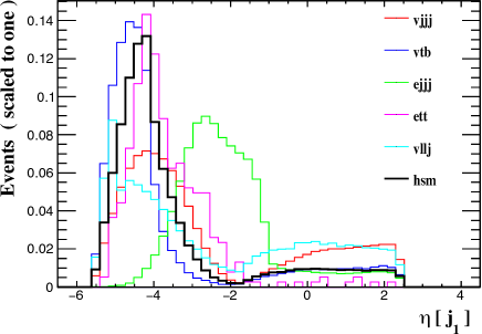
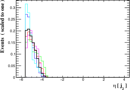
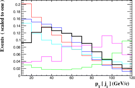
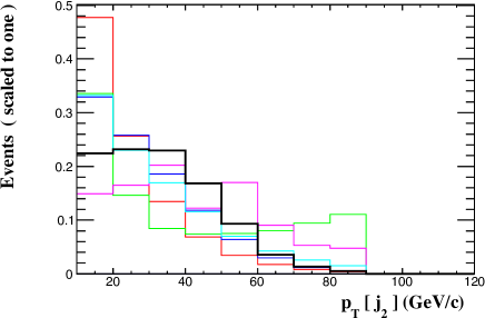
Figure 3: Top-left) Jet pseudorapidity distribution for the first jet. Top-right) Same for the second jet. Bottom-left) Transverse momentum distribution for the first jet. Bottom-right) Same for the second jet. These histograms are made for the Ia incarnation of the 2HDM-III signal as well as the five categories of background discussed in the text.

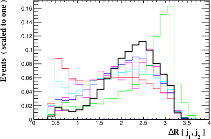
Figure 4: Jet separation distribution. These histograms are made for the Ia incarnation of the 2HDM-III signal as well as the five categories of background discussed in the text.

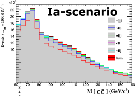
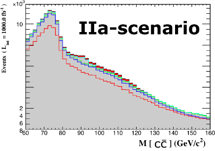
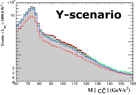
Figure 5: Di-jet invariant mass distribution. These histograms are made for the Ia (top-left), IIa (top-right) and Y (bottom) incarnations of the 2HDM-III signal (red histogram) as well as the five categories of background discussed in the text (here stacked beneath the signal). Here, we present the rates for the case of $c\bar{c}$-tagged sample.

Signal	Raw events	Sim Events	Set A)	Set B)	Set C)	Set D)	Set E)	Significance
Ia	875000	890530	633866	190986	91117	77079	36054	36.3
			36075	10869	5186	4387	2052	8.31
IIa	958000	970336	609152	178088	87714	72312	30898	31.19
			32350	9457	4658	3840	1641	6.67
Y	1070000	1085244	736138	208665	101427	83083	35824	36.08
			41941	11884	5776	4732	2040	8.27
$\Sigma\nu 3j$	$1.89\times 10^{8}$	19956113	176368197	40956844	9327890	4960087	820718
			10334771	2399977	546593	290650	48092
$\nu tb$	$1.24\times 10^{7}$	1254485	7880059	1505048	759201	548492	123961
			501285	95743	48296	34892	7886	$\Sigma\;B=$
$\Sigma e3j$	$10^{9}$	104495242	73393857	3093729	29137	24770	2750	950207
			52792574	2225334	20958	17817	1978	$58865$
$ett$	$350000$	353583	26046	380	109	77	21
			14764	215	62	44	12
$\Sigma\nu llj$	$3090000$	1434318	411923	117562	29915	19052	2757
			134029	38253	9733	6199	897

Table 5: Cutflow for all signals and backgrounds. Here, in each cell, the top line represents the number of light di-jet events while the bottom one refers to those enriched by $c\bar{c}$ states, as described in the text.

V Conclusions

In summary, we have studied the process $e^{-}p\to\nu_{e}hq$ assuming the decay channel $h\to c\bar{c}$, where $h$ is the discovered SM-like state, at a FCC-eh with $E_{b}=50$ TeV and $E_{e^{-}}=60$ GeV in presence of a $-80\%$ polarisation of the $e^{-}$ beam. We considered this channel in the context of a 2HDM-III embedding a four-zero texture in the Yukawa matrices and a general Higgs potential, where both Higgs doublets are coupled with up- and down-type fermions, as a theoretical framework that can be mapped into the standard four types of 2HDM. Hence, we have defined three limits of it reproducing the Type I, II and Y (but not X, which offers no sensitivity to our study) setups. The purpose was to show that this collider has the ability to access the Yukawa coupling between the SM-like Higgs state and $c$-quarks, which can only be determined with significant errors at present and future hadronic machines, like the (HL-)LHC and FCC-hh.

Upon accounting for flavour mistagging effects in a realistic way in presence of parton shower, hadronisation and detector effects and simulating both reducible and irreducible backgrounds, we have proven that large significances can be achieved at such FCC-eh, above and beyond what attainable at the aforementioned hadronic machines and comparable to the FCC-ee expectations. This conclusion applies to all three 2HDM-III incarnations discussed, each being exemplified by two BPs at the edges of the currently allowed (by LHC data) interval on the Yukawa coupling between the SM-like Higgs state and $b$-quarks.

References

- Moretti and Stirling (1995) S. Moretti and W. J. Stirling, Phys. Lett. B 347, 291 (1995), [Erratum: Phys. Lett. B 366, 451 (1996)].
- Li et al. (2021) S.-Y. Li, Z.-Y. Li, P.-C. Lu, and Z.-G. Si, Chin. Phys. C 45, 093105 (2021).
- Branco et al. (2012) G. C. Branco, P. M. Ferreira, L. Lavoura, M. N. Rebelo, M. Sher, and J. P. Silva, Phys. Rept. 516, 1 (2012).
- Barger et al. (1990) V. D. Barger, J. L. Hewett, and R. J. N. Phillips, Phys. Rev. D 41, 3421 (1990).
- Grossman (1994) Y. Grossman, Nucl. Phys. B 426, 355 (1994), arXiv:hep-ph/9401311 .
- Aoki et al. (2009) M. Aoki, S. Kanemura, K. Tsumura, and K. Yagyu, Phys. Rev. D 80, 015017 (2009), arXiv:0902.4665 [hep-ph] .
- Gunion et al. (2000) J. F. Gunion, H. E. Haber, G. L. Kane, and S. Dawson, Front. Phys. 80 (2000).
- Donoghue and Li (1979) J. F. Donoghue and L. F. Li, Phys. Rev. D 19, 945 (1979).
- Barnett et al. (1984) R. M. Barnett, G. Senjanovic, and D. Wyler, Phys. Rev. D 30, 1529 (1984).
- Fritzsch and Xing (2003) H. Fritzsch and Z.-z. Xing, Phys. Lett. B 555, 63 (2003).
- Diaz-Cruz et al. (2009) J. L. Diaz-Cruz, J. Hernandez-Sanchez, S. Moretti, R. Noriega-Papaqui, and A. Rosado, Phys. Rev. D 79, 095025 (2009).
- Hernández-Sánchez et al. (2017) J. Hernández-Sánchez, O. Flores-Sánchez, C. G. Honorato, S. Moretti, and S. Rosado, PoS CHARGED2016, 032 (2017).
- Hernandez-Sanchez et al. (2012) J. Hernandez-Sanchez, S. Moretti, R. Noriega-Papaqui, and A. Rosado, PoS CHARGED2012, 029 (2012).
- Hernandez-Sanchez et al. (2015) J. Hernandez-Sanchez, S. P. Das, S. Moretti, A. Rosado, and R. Xoxocotzi-Aguilar, PoS DIS2015, 227 (2015).
- Das et al. (2016) S. P. Das, J. Hernández-Sánchez, S. Moretti, A. Rosado, and R. Xoxocotzi, Phys. Rev. D 94, 055003 (2016).
- Hernandez-Sanchez et al. (2013) J. Hernandez-Sanchez, S. Moretti, R. Noriega-Papaqui, and A. Rosado, JHEP 07, 044 (2013).
- Akeroyd et al. (2017) A. G. Akeroyd et al., Eur. Phys. J. C 77, 276 (2017).
- Akeroyd et al. (2012) A. G. Akeroyd, S. Moretti, and J. Hernandez-Sanchez, Phys. Rev. D 85, 115002 (2012).
- Gianotti et al. (2005) F. Gianotti et al., Eur. Phys. J. C39, 293 (2005).
- Apollinari et al. (2017) G. Apollinari, I. Béjar Alonso, O. Brüning, P. Fessia, M. Lamont, L. Rossi, and L. Tavian, CERN-2017-007-M 4/2017 (2017).
- Kuze (2018) M. Kuze, Int. J. Mod. Phys. Conf. Ser. 46, 1860081 (2018).
- Britzger and Klein (2018) D. Britzger and M. Klein, PoS DIS2017, 105 (2018).
- Abada et al. (2019a) A. Abada et al. (FCC), Eur. Phys. J. C79, 474 (2019a).
- Abada et al. (2019b) A. Abada et al. (FCC), Eur. Phys. J. ST 228, 755 (2019b).
- Jueid et al. (2021) A. Jueid, J. Kim, S. Lee, and J. Song, Phys. Lett. B 819, 136417 (2021).
- Haber and Hempfling (1993) H. E. Haber and R. Hempfling, Phys. Rev. D 48, 4280 (1993), arXiv:hep-ph/9307201 .
- Gunion and Haber (2003) J. F. Gunion and H. E. Haber, Phys. Rev. D 67, 075019 (2003).
- Dubinin and Semenov (2003) M. N. Dubinin and A. V. Semenov, Eur. Phys. J. C 28, 223 (2003), arXiv:hep-ph/0206205 .
- Gunion and Haber (2005) J. F. Gunion and H. E. Haber, Phys. Rev. D 72, 095002 (2005), arXiv:hep-ph/0506227 .
- Cordero-Cid et al. (2014) A. Cordero-Cid, J. Hernandez-Sanchez, C. G. Honorato, S. Moretti, M. A. Perez, and A. Rosado, JHEP 07, 057 (2014).
- Gerard and Herquet (2007) J. M. Gerard and M. Herquet, Phys. Rev. Lett. 98, 251802 (2007).
- Toussaint (1978) D. Toussaint, Phys. Rev. D 18, 1626 (1978).
- Bertolini (1986) S. Bertolini, Nucl. Phys. B 272, 77 (1986).
- Hollik (1986) W. Hollik, Z. Phys. C 32, 291 (1986).
- Gunion and Turski (1989) J. F. Gunion and A. Turski, Phys. Rev. D 39, 2701 (1989).
- de Visscher et al. (2009) S. de Visscher, J.-M. Gerard, M. Herquet, V. Lemaitre, and F. Maltoni, JHEP 08, 042 (2009).
- Haller et al. (2018) J. Haller, A. Hoecker, R. Kogler, K. Mönig, T. Peiffer, and J. Stelzer, Eur. Phys. J. C 78, 675 (2018).
- Kanemura et al. (2011) S. Kanemura, Y. Okada, H. Taniguchi, and K. Tsumura, Phys. Lett. B 704, 303 (2011).
- Zyla et al. (2020) P. Zyla et al. (Particle Data Group), PTEP 2020, 083C01 (2020).
- Félix-Beltrán et al. (2015) O. Félix-Beltrán, F. González-Canales, J. Hernández-Sánchez, S. Moretti, R. Noriega-Papaqui, and A. Rosado, Phys. Lett. B 742, 347 (2015).
- Aranda et al. (2012) A. Aranda, C. Bonilla, and A. D. Rojas, Phys. Rev. D 85, 036004 (2012).
- Branco et al. (2010) G. Branco, D. Emmanuel-Costa, and C. Simões, Phys. Lett. B 690, 62 (2010).
- Botella et al. (2013) F. Botella, G. Branco, and M. Rebelo, Phys. Lett. B 722, 76 (2013).
- Frigerio et al. (2005) M. Frigerio, S. Kaneko, E. Ma, and M. Tanimoto, Phys. Rev. D 71, 011901 (R) (2005).
- Cordero-Cid et al. (2015) A. Cordero-Cid, J. Hernádez-Sánchez, C. Honorato, and S. Moretti, PoS Charged2014, 026 (2015).
- Casalbuoni et al. (1986) R. Casalbuoni, D. Dominici, R. Gatto, and C. Giunti, Phys. Lett. B 178, 235 (1986).
- Ginzburg and Ivanov (2005) I. F. Ginzburg and I. P. Ivanov, Phys. Rev. D 72, 115010 (2005), arXiv:hep-ph/0508020 .
- Ferreira et al. (2004) P. M. Ferreira, R. Santos, and A. Barroso, Phys. Lett. B 603, 219 (2004), [Erratum: Phys.Lett.B 629, 114–114 (2005)], arXiv:hep-ph/0406231 .
- Ivanov (2008) I. P. Ivanov, Phys. Rev. D 77, 015017 (2008), arXiv:0710.3490 [hep-ph] .
- Hernández-Sánchez et al. (2020) J. Hernández-Sánchez, C. G. Honorato, S. Moretti, and S. Rosado-Navarro, Phys. Rev. D 102, 055008 (2020).
- Crivellin et al. (2013) A. Crivellin, C. Greub, and A. Kokulu, Phys. Rev. D 87, 094031 (2013).
- Aad et al. (2020a) G. Aad et al. (ATLAS), Phys. Rev. D 101, 012002 (2020a).
- Aad et al. (2016) G. Aad et al. (ATLAS, CMS), JHEP 08, 045 (2016).
- Sirunyan et al. (2019a) A. M. Sirunyan et al. (CMS), Eur. Phys. J. C 79, 421 (2019a).
- Sirunyan et al. (2020) A. M. Sirunyan et al. (CMS), JHEP 03, 055 (2020).
- Khachatryan et al. (2016) V. Khachatryan et al. (CMS), Phys. Lett. B 759, 369 (2016).
- Abbiendi et al. (2013) G. Abbiendi et al. (ALEPH, DELPHI, L3, OPAL, LEP), Eur. Phys. J. C 73, 2463 (2013).
- Abbott et al. (1999) B. Abbott et al. (D0), Phys. Rev. Lett. 82, 4975 (1999).
- Abulencia et al. (2006) A. Abulencia et al. (CDF), Phys. Rev. Lett. 96, 042003 (2006).
- Abazov et al. (2009) V. M. Abazov et al. (D0), Phys. Lett. B 682, 278 (2009).
- Sirunyan et al. (2018a) A. M. Sirunyan et al. (CMS), JHEP 11, 115 (2018a), arXiv:1808.06575 [hep-ex] .
- Sirunyan et al. (2019b) A. M. Sirunyan et al. (CMS), JHEP 07, 142 (2019b).
- Aaboud et al. (2018a) M. Aaboud et al. (ATLAS), Phys. Lett. B 784, 345 (2018a).
- Aaboud et al. (2018b) M. Aaboud et al. (ATLAS), Phys. Lett. B 786, 114 (2018b).
- Aad et al. (2020b) G. Aad et al. (ATLAS), Phys. Lett. B 809, 135754 (2020b).
- Aaboud et al. (2017) M. Aaboud et al. (ATLAS), JHEP 10, 112 (2017).
- Sirunyan et al. (2019c) A. M. Sirunyan et al. (CMS), Eur. Phys. J. C 79, 421 (2019c).
- Sirunyan et al. (2018b) A. M. Sirunyan et al. (CMS), JHEP 11, 152 (2018b).
- Flores-Sánchez et al. (2019) O. Flores-Sánchez, J. Hernández-Sánchez, C. G. Honorato, S. Moretti, and S. Rosado-Navarro, Phys. Rev. D 99, 095009 (2019).
- Workman and Others (2022) R. L. Workman and Others (Particle Data Group), PTEP 2022, 083C01 (2022).
- Sopczak (2020) A. Sopczak (ATLAS, CMS), PoS FFK2019, 006 (2020).
- Aaboud et al. (2018c) M. Aaboud et al. (ATLAS), Phys. Lett. B 786, 59 (2018c).
- Sirunyan et al. (2018c) A. M. Sirunyan et al. (CMS), Phys. Rev. Lett. 121, 121801 (2018c).
- Aad et al. (2022) G. Aad et al. (ATLAS), Eur. Phys. J. C 82, 717 (2022), arXiv:2201.11428 [hep-ex] .
- CMS (2022) (2022), arXiv:2205.05550 [hep-ex] .
- Andersen et al. (2013) J. R. Andersen et al. (LHC Higgs Cross Section Working Group), (2013), 10.5170/CERN-2013-004, arXiv:1307.1347 [hep-ph] .
- de Florian et al. (2016) D. de Florian et al. (LHC Higgs Cross Section Working Group), 2/2017 (2016), 10.23731/CYRM-2017-002, arXiv:1610.07922 [hep-ph] .
- U. Klein et al. (2014) U. Klein et al., “ Meeting of the Physics Convenors of the LHeC, Higgs at LHeC/FCC-he conferences,” (2014), https://indico.cern.ch/event/350727/contributions/826001/attachments/693294/.
- Belyaev et al. (2013) A. Belyaev, N. D. Christensen, and A. Pukhov, Comput. Phys. Commun. 184, 1729 (2013).
- Pumplin et al. (2002) J. Pumplin, D. R. Stump, J. Huston, H. L. Lai, P. M. Nadolsky, and W. K. Tung, JHEP 07, 012 (2002).
- Agostini et al. (2020) P. Agostini et al. (LHeC, FCC-he Study Group), JLAB-ACP-20-3180 (2020).
- Aihara et al. (2019) H. Aihara et al. (ILC), (2019), arXiv:1901.09829 [hep-ex] .
- et al. (2018) M. A. et al. (CLIC accelerator), 4/2018 (2018), 10.23731/CYRM-2018-004, arXiv:1903.08655 [physics.acc-ph] .
- Sjöstrand et al. (2015) T. Sjöstrand, S. Ask, J. R. Christiansen, R. Corke, N. Desai, P. Ilten, S. Mrenna, S. Prestel, C. O. Rasmussen, and P. Z. Skands, Comput. Phys. Commun. 191, 159 (2015).
- de Favereau et al. (2014) J. de Favereau, C. Delaere, P. Demin, A. Giammanco, V. Lemaître, A. Mertens, and M. Selvaggi (DELPHES 3), JHEP 02, 057 (2014).
- U. Klein et al. (2017) U. Klein et al., “Final FCChe delphes card & discussion, Higgs & Top at LHeC conferences,” (2017), https://indico.cern.ch/event/624658/.
- Conte et al. (2013) E. Conte, B. Fuks, and G. Serret, Comput. Phys. Commun. 184, 222 (2013).
- Abada et al. (2019c) A. Abada et al. (FCC), Eur. Phys. J. ST 228, 755 (2019c).
- Abada et al. (2019d) A. Abada et al. (FCC), Eur. Phys. J. ST 228, 261 (2019d).