July, 2023

ABSTRACT

Single index models provide an effective dimension reduction tool in regression, especially for high dimensional data, by projecting a general multivariate predictor onto a direction vector. We propose a novel single-index model for regression models where metric space-valued random object responses are coupled with multivariate Euclidean predictors. The responses in this regression model include complex, non-Euclidean data, including covariance matrices, graph Laplacians of networks, and univariate probability distribution functions, among other complex objects that lie in abstract metric spaces. While Fréchet regression has proved useful for modeling the conditional mean of such random objects given multivariate Euclidean vectors, it does not provide for regression parameters such as slopes or intercepts, since the metric space-valued responses are not amenable to linear operations. As a consequence, distributional results for Fréchet regression have been elusive. We show here that for the case of multivariate Euclidean predictors, the parameters that define a single index and projection vector can be used to substitute for the inherent absence of parameters in Fréchet regression. Specifically, we derive the asymptotic distribution of suitable estimates of these parameters, which then can be utilized to test linear hypotheses for the parameters, subject to an identifiability condition. Consistent estimation of the link function of the single index Fréchet regression model is obtained through local linear Fréchet regression. We demonstrate the finite sample performance of estimation and inference for the proposed single index Fréchet regression model through simulation studies, including the special cases where responses are probability distributions and graph adjacency matrices. The method is illustrated for resting-state functional Magnetic Resonance Imaging (fMRI) data from the ADNI study.

KEY WORDS: Single index, Dimension reduction, Random objects, Non-Euclidean data, Local Fréchet regression, M-estimation, FMRI.

1 Introduction

Modeling the regression relationship between a real-valued response $Y$ and a multivariate Euclidean predictor vector X corresponds to specifying the form of the conditional means $m(\textbf{x})=\mathbb{E}{(Y|\textbf{X}=\textbf{x})}.$ Higher dimensionality of X can be problematic when one is interested to go beyond the standard multiple linear models and aims for a nonparametric estimation of $m(\textbf{x}).$ This provides strong motivation to consider regression models that provide dimension reduction. Single index models are one of the most popular approaches to achieve this under the assumption that the influence of the predictors on the response can be collapsed to a single index, i.e., a projection on a specific direction, complemented by a nonparametric link function. This reduces the predictors to a univariate index while still capturing relevant features and since the nonparametric link function acts only on a one-dimensional index, these models are not subject to the curse of dimensionality. The single index model generalizes linear regression, where the link function is the identity. For a real-valued response, $Y$ and a $p$-dimensional predictor X, the semiparametric single index regression model is given by

$$\begin{gathered}\mathbb{E}{(Y|\textbf{X}=\textbf{x})}=\mathbb{E}{(Y|\textbf{X}^{\top}{\bm{\bar{\theta}_{0}}}=t)}=m(t,{\bm{\bar{\theta}_{0}}}).\end{gathered}$$ (1)

In model (1), the dependence between $Y$ and $\textbf{X},$ characterized by the conditional mean, is summarized by the parameter vector ${\bm{\bar{\theta}_{0}}}$ and the link function $m$.

The function $m$ is nonparametric and thus includes location and level changes, and therefore the vector X cannot include a constant that would serve as an intercept. For identifiability reasons, ${\bm{\bar{\theta}_{0}}}$ is often assumed to be a unit vector with a positive first coordinate. A second approach is to require one component to equal one. This presupposes that the component that is set to equal 1 indeed has a non-zero coefficient (Lin and Kulasekera,, 2007; Cui et al.,, 2011). Model (1) is only meaningful if the Euclidean predictor vector X is of dimension $2$ or larger. If X is one-dimensional, the corresponding special case of the model is the one-dimensional nonparametric regression $\mathbb{E}{(Y|X=x)}=m(x)$, which does not feature any parametric component.

The classical single index regression model with Euclidean responses has attracted attention from the scientific community for a long time due to its flexibility and the interpretability of the (linear) coefficients and flexibility, owing to the nonparametric link function, as well as due to its wide applicability in many scientific fields. The coefficient ${\bm{\bar{\theta}_{0}}}$ that defines the single index $\textbf{x}^{\top}{\bm{\bar{\theta}_{0}}}$ along with the shape of the nonparametric component $m$ characterizes the relationship between the response and the predictor. The parametric component ${\bm{\bar{\theta}_{0}}}$ is of primary interest for inference in this model. The problem of recovering the true direction ${\bm{\bar{\theta}_{0}}}$ can be viewed as a subclass of sufficient dimension reduction (SDR) techniques, where identifying the central subspace of X that explains most of the variation in $Y$ has been a prime target (Li and Duan,, 1989; Cook,, 1994; Li and Wang,, 2007).

In addition to sufficient dimension reduction techniques, various related approaches to estimate ${\bm{\bar{\theta}_{0}}}$ in (1) have been studied. These include projection pursuit regression (PPR) (Friedman and Stuetzle,, 1981; Hall,, 1989), average derivatives (Härdle and Stoker,, 1989; Stoker,, 1986), sliced inverse regression (SIR) (Li,, 1991), conditional minimum average variance estimation (MAVE) (Xia et al.,, 2009) and various other methods (Xia and Härdle,, 2006; Xia,, 2007). These approaches have focused on the nonparametric estimation of the link function to recover the index parameter in (1) (Härdle et al.,, 1993; Huh and Park,, 2002; Hristache et al.,, 2001), partially linear versions (Carroll et al.,, 1997; Yu and Ruppert,, 2002) and various noise models (Chang et al.,, 2010; Wang et al.,, 2010). Inference for the index parameters has also been well studied (Fan and Huang,, 2005; Liang et al.,, 2010; Gao and Liang,, 1997) for the classical single index model.

Various extensions of single index regression have been considered more recently (Zhao et al.,, 2020; Kereta et al.,, 2020), including models with multiple indices or high-dimensional predictors (Zhu and Zhu,, 2009; Zhou and He,, 2008; Kuchibhotla and Patra,, 2020), censored data (Lopez et al.,, 2013), and longitudinal and functional data as predictors (Jiang and Wang,, 2011; Chen et al.,, 2011; Ferraty et al.,, 2011; Novo et al.,, 2019). However, none of these extensions has covered situations where responses are not in a Euclidean vector space, even though this case is increasingly important for data analysis. Two very recent exceptions are Ying and Yu, (2020) and Zhang et al., (2021), who considered extending sufficient dimension reduction approaches for the case of random objects. The overall lack of available methodology for single-index models with random object responses motivates our approach. Non-Euclidean complex data structures arising in areas such as biological or social sciences are becoming increasingly common, due to technological advances that have made it possible to record and efficiently store sensor data and images (Peyré,, 2009), shapes (Small,, 2012) or networks (Tsochantaridis et al.,, 2004). For example, one might be interested in functional connectivity, quantified in the form of correlation matrices obtained from neuroimaging studies, to study the effect of predictors on brain connectivity, an application that we explore in Section 5.1.

Other examples of general metric space objects include probability distributions (Delicado and Vieu,, 2017), such as age-at-death distributions as observed in demography or network objects, such as internet traffic networks. Such “object-oriented data” (Marron and Alonso,, 2014) or “random objects” (Müller,, 2016) can be viewed as random variables taking values in a separable metric space that is devoid of a vector space structure and where only pairwise distances between the observed data are available. Almost all existing methodology for single-index models as briefly reviewed above assumes that one has Euclidean responses, and these methods rely in a fundamental way on the vector space structure of the space where the responses reside. When there is no linear structure, a new methodology is needed and this paper contributes to this development.

A natural measure of location for random elements of a metric space is the Fréchet mean (Fréchet,, 1948), which is a direct generalization of the standard mean and is defined as the element of the metric space for which the expected squared distance to all other elements, known as the Fréchet function, is minimized. Depending on the space and metric, Fréchet means may or may not exist as unique minimizers of the Fréchet function. Fréchet regression is an extension of Fréchet means to the notion of conditional Fréchet means, and local as well as global versions have been recently studied in several papers (Petersen and Müller,, 2019; Petersen et al.,, 2019; Schötz,, 2019, 2020; Bhattacharjee and Müller,, 2022).

Global Fréchet regression is a generalization of linear regression for random object responses. In analogy to classical linear regression, it features a restrictive structural model assumption. While the local linear version of Fréchet regression is more flexible, it suffers from the curse of dimensionality as the dimension of the predictors increases. Further, neither version of the Fréchet regression incorporates an interpretable inference regime. In this paper, we introduce (single) Index Fréchet Regression (IFR) to facilitate inference in the context of Fréchet regression when the response variable is a random object lying in general metric space and the predictor is a $p$-dimensional Euclidean vector X with $p\geq 1.$ Our goal is to develop an extension of the conventional estimation and inference paradigm for single-index models for this challenging case. It is assumed that the conditional expectation (Fréchet regression) of $Y$ depends on the predictor vector X only through the projection or index $\textbf{X}^{\top}{\bm{\bar{\theta}_{0}}}$ for a parameter vector ${\bm{\bar{\theta}_{0}}}\in\bar{\Theta}\in\mathbb{R}^{p}.$ Since there is no notion of direction or sign in a general metric space, we interpret the index parameter in the proposed index Fréchet regression model (IFR) as the direction in the predictor space along which the variability of the response is maximized. The semiparametric framework provided by the proposed single index model facilitates stable estimation and interpretable inference.

It turns out to be useful to cast the direction estimation problem in the framework of M-estimation for an appropriate objective function and to use empirical process theory to show consistency of the proposed estimate. We derive an asymptotic normality result for these estimators under mild assumptions on the metric space and the unknown link function by utilizing an appropriate version of recent results of Chen and Müller, (2022) concerning local linear Fréchet regression estimators. Under suitable regularity assumptions, the asymptotic distribution of the estimated index parameter can then be harnessed to construct a Wald-type statistic to conduct inference. Combining this with an auxiliary result on the asymptotic convergence of the estimated covariance matrix makes it possible to employ a bootstrap method to obtain inference in finite sample situations.

When we finalized this work, we became aware that independently and simultaneously another group also developed an approach for single index Fréchet regression (Ghosal et al.,, 2021). We wish to emphasize that this paper was not in any way influenced by this parallel development (with preprints becoming available within days of each other).

The paper is organized as follows: The basic setup is defined in Section 2 and the theory on the asymptotic behavior of the index parameter is provided in Section 3, with a focus on results for inference. The index vector is assumed to lie on a hyper-sphere, with a non-negative first element to facilitate identifiability. Then it is natural to quantify the performance of the proposed estimators by the geodesic distances between the estimated and true directions. The results of simulation studies with various types of random objects as responses are reported in Section 4 with additional results in the Supplement. In Section 5 we apply the methods to infer and analyze the effect of age, sex, total Alzheimer’s brain score and the stage of Alzheimer’s Disease on the brain connectivity of patients with dementia. Brain connectivity is derived from fMRI signals of brain regions of interest (Thomas Yeo et al.,, 2011) and quantified in the form of correlation matrix objects. We present additional illustrations for human mortality data as distributional objects and mood data of unemployed workers as compositional objects, with details in the Supplement. A brief discussion follows in Section 6.

2 Model and Estimation Methods

In all of the following, $(\Omega,d,P)$ is a totally bounded metric space with metric $d$ and a probability measure $P.$ The random objects $Y$ take values in $\Omega$. This is coupled with a $p$-dimensional real-valued predictor $\textbf{X}.$ Throughout we will use bold letters to denote multivariate real vectors. The conditional Fréchet mean of $Y$ given X is a generalization of $\mathbb{E}{(Y|\textbf{X}=\textbf{x})}$ to metric spaces, defined as the argmin of $\mathbb{E}{(d^{2}(Y,\omega)|\textbf{X}=\textbf{x})},$ $\omega\in\Omega$ (Petersen and Müller,, 2019), i.e.,

$$\mathbb{E}_{\oplus}{(Y|\textbf{X}=\textbf{x})}:=\underset{\omega\ \in\ \Omega}{\operatorname*{argmin}}\ \mathbb{E}{(d^{2}(Y,\omega)|\textbf{X}=\textbf{x})}.$$ (2)

Evaluated at the minimizer, the objective function in (2) is the corresponding generalized measure of dispersion around the conditional Fréchet mean and can be viewed as a conditional Fréchet function.

As discussed earlier, obtaining inference for Fréchet regression is an elusive goal, for both the more restrictive global as well as the more flexible but the curse of dimensionality afflicted local version of Fréchet regression. To move towards inference, we propose here a more structured model, inspired by its Euclidean single index equivalent in (1), given by

$$\mathbb{E}_{\oplus}{(Y|\textbf{X}=\textbf{x})}=m_{\oplus}(\textbf{x}^{\top}{\bm{\bar{\theta}_{0}}},{\bm{\bar{\theta}_{0}}}),$$ (3)

where ${\bm{\bar{\theta}_{0}}}$ is the true direction parameter of interest. Model (1) emerges as a special case of model (3) for a Euclidean response, as the conditional Fréchet mean coincides with the conditional expectation $\mathbb{E}{(Y|\textbf{X})}$ for the choice of the absolute Euclidean distance metric for the case $\Omega=\mathbb{R}.$ In other words, the conditional Fréchet mean is assumed to be a function of ${\bm{\bar{\theta}_{0}}}$ in such a way that the distribution of $Y$ only depends on X only through the index $\textbf{X}^{\top}{\bm{\bar{\theta}_{0}}},$ that is, $Y\perp\mathbb{E}_{\oplus}{(Y|\textbf{X})}|(\textbf{X}^{\top}{\bm{\bar{\theta}_{0}}}).$ Thus

$$\mathbb{E}_{\oplus}{(Y|\textbf{X}=\textbf{x})}=\mathbb{E}_{\oplus}{(Y|\textbf{X}^{\top}{\bm{\bar{\theta}_{0}}}=t)}=m_{\oplus}(t,{\bm{\bar{\theta}_{0}}}),$$

and invoking local linear nonparametric Fréchet regression for the one-dimensional index promises to overcome the curse of dimensionality problem. For projections $\textbf{X}^{\top}{\bm{\bar{\theta}_{0}}}\in\mathcal{T}_{{\bm{\bar{\theta}_{0}}}}\subset\mathbb{R}$, which depend on ${\bm{\bar{\theta}_{0}}}$, we consider predictors X with bounded norm such that $\mathcal{T}_{{\bm{\bar{\theta}_{0}}}}\subset\mathcal{T}$, where $\mathcal{T}$ is a compact interval on $\mathbb{R}.$ We note that the link function, for given ${\bm{\bar{\theta}_{0}}}\in\bar{\Theta},$ $m_{\oplus}:\mathcal{T}_{{\bm{\bar{\theta}_{0}}}}\mapsto(\Omega,d)$ in the true model depends on the multivariate predictor $\textbf{X}=\textbf{x}$ only through the single-index $t=\textbf{x}^{\top}{\bm{\bar{\theta}_{0}}}$, as well as on the direction vector ${\bm{\bar{\theta}_{0}}}$ implicitly. Thus, explicitly characterizing this dependence, we define the Index Fréchet Regression (IFR) model for random object response $Y$ and Euclidean predictor X as

$$m_{\oplus}(t,{\bm{\bar{\theta}_{0}}}):=\underset{\omega\ \in\ \Omega}{\operatorname*{argmin}}\ \mathbb{E}{(d^{2}(Y,\omega)|\textbf{X}^{\top}{\bm{\bar{\theta}_{0}}}=t)}.$$ (4)

The coefficient ${\bm{\bar{\theta}_{0}}}\in\mathbb{R}^{p}$ is the quantity of interest for the single index Fréchet model owing to its interpretability by quantifying the contribution of each predictor component. More generally, the quantity in model (4) can be evaluated for any direction vector $\bm{\bar{\theta}}\in\bar{\Theta}$ by

$$m_{\oplus}(\textbf{x}^{\top}\bm{\bar{\theta}},\bm{\bar{\theta}})=\underset{\omega\ \in\ \Omega}{\operatorname*{argmin}}\ \mathbb{E}{(d^{2}(Y,\omega)|\textbf{X}^{\top}\bm{\theta}=\textbf{x}^{\top}\bm{\bar{\theta}})}.$$ (5)

In the Euclidean case, identifiability conditions for the direction parameter have been widely discussed in the literature (Carroll et al.,, 1997; Lin and Kulasekera,, 2007; Cui et al.,, 2011; Zhu and Xue,, 2006). We assume the parameter space $\bar{\Theta}$ to be constrained in order to ensure that $\bm{\bar{\theta}}$ in the representation (5) is uniquely defined, where

$$\bar{\Theta}:=\{\bm{\bar{\theta}}=(\theta_{1},\dots,\theta_{p})^{\top}:\|\bm{\bar{\theta}}\|=1,\ \theta_{1}>0,\ \bm{\bar{\theta}}\in\mathbb{R}^{p}\}.$$ (6)

We first choose an identifiable parametrization that transforms the boundary of a unit ball in $\mathbb{R}^{p}$ to the interior of a unit ball in $\mathbb{R}^{(p-1)}$. By eliminating $\theta_{1},$ the parameter space $\bar{\Theta}$ can be rearranged to $\{((1-\sum_{r=2}^{p}\theta_{r}^{2})^{1/2},\theta_{2},\dots,\theta_{p})^{\top}:\sum_{r=2}^{p}\theta_{r}^{2}<1\}.$ This re-parametrization is the key to analyzing the asymptotic properties of the estimates for $\bm{\theta}$ and also facilitating efficient computation. The true parameter is then partitioned into $\bm{\bar{\theta}}=(\theta_{1},\bm{\theta})^{\top},$ where $\bm{\theta}=(\theta_{2},\dots,\theta_{p})^{\top}.$ We estimate the $(p-1)-$ dimensional vector $\bm{\theta}$ in the single-index model and then use $\theta_{1}=(1-\sum_{r=2}^{p}\theta_{r}^{2})^{1/2}$ to obtain $\hat{\theta}_{1}.$

Proposition 1 (Identifiability of model (4)).

Suppose $h_{\oplus}({\textbf{x}})=\mathbb{E}_{\oplus}{(Y|\textbf{X}=\textbf{x})}$, that the support $S$ of $h_{\oplus}({\cdot})$ is a convex bounded set with at least one interior point and that $h_{\oplus}({\cdot})$ is a non-constant continuous function on $S.$ If

$$h_{\oplus}(\textbf{x})=g_{1\oplus}(\bm{\alpha}^{\top}\textbf{x},\bm{\alpha})=g_{2\oplus}(\bm{\beta}^{\top}\textbf{x},\bm{\beta}),\text{ for all }\textbf{x}\in S,$$

for some continuous object-valued link functions $g_{1\oplus}$ and $g_{2\oplus}$, and some $\bm{\alpha},\bm{\beta}\in\bar{\Theta},$ where $\bar{\Theta}$ is as described in (6). Then $\bm{\alpha}=\bm{\beta}$ and $g_{1\oplus}\equiv g_{2\oplus}$ on $\{\bm{\alpha}^{\top}\textbf{x}|\textbf{x}\in S\}.$

The above result can be proved using a similar argument as given in the proof of Theorem $1$ of Lin and Kulasekera, (2007).

Scrutinizing the special case of a Euclidean response $Y$ in model (1), the variation in $Y$ is seen to result from the variation in $\textbf{X}^{\top}{\bm{\bar{\theta}_{0}}}$ as well as from the variation in the error term in the model, denoted by $\varepsilon$ (Ichimura,, 1993). On the contour line $\textbf{X}^{\top}{\bm{\bar{\theta}_{0}}}=c$, the variability in $Y$ only results from the variability in $\varepsilon$. Along contour lines $\textbf{X}^{\top}\bm{\bar{\theta}}=c$ for $\bm{\bar{\theta}}\neq{\bm{\bar{\theta}_{0}}}$, $\textbf{X}^{\top}{\bm{\bar{\theta}_{0}}}$ is not constant and therefore the variability in $Y$ along the contour lines $\textbf{X}^{\top}\bm{\bar{\theta}}=c,\ \bm{\bar{\theta}}\neq{\bm{\bar{\theta}_{0}}}$ is due to both the variation in $\textbf{X}^{\top}{\bm{\bar{\theta}_{0}}}$ and in $\varepsilon$. Since ${\rm Var}\left(Y|\textbf{X}^{\top}\bm{\bar{\theta}}=c\right)$ measures the variability in $Y$ on a contour line $\textbf{X}^{\top}\bm{\bar{\theta}}=c,\ \bm{\bar{\theta}}\neq{\bm{\bar{\theta}_{0}}}$, one can characterize ${\bm{\bar{\theta}_{0}}}$ as the minimizer of the objective function $H(\bm{\bar{\theta}})$, where $H(\bm{\bar{\theta}}):=\mathbb{E}{({\rm Var}(Y|\textbf{X}^{\top}\bm{\bar{\theta}}))}\text{ and }{\bm{\bar{\theta}_{0}}}=\operatorname*{argmin}_{\bm{\bar{\theta}}\in\bar{\Theta}}H(\bm{\bar{\theta}}).$ The constraint $\bm{\bar{\theta}}^{\top}\bm{\bar{\theta}}=1,$ with the first element of the index $\theta_{1}>0$, ensures the identifiability of the objective function. Defining an equivalence class of the parameter vector $\bar{\Theta}_{{\bm{\bar{\theta}_{0}}}}:=\{\bm{\bar{\theta}}\in\bar{\Theta}:m(\textbf{x}^{\top}\bm{\bar{\theta}})=m(\textbf{x}^{\top}{\bm{\bar{\theta}_{0}}})\text{ a.e. in }\textbf{x}\text{ for some }m\}$ for $\bm{\bar{\theta}}\notin\bar{\Theta}_{{\bm{\bar{\theta}_{0}}}}$, one has $H({\bm{\bar{\theta}_{0}}})<H(\bm{\bar{\theta}}).$

To recover the true direction of the single index from model (4), the conditional variance of $Y$ given $\textbf{X}=\textbf{x}$ for a real-valued response can be replaced by the conditional Fréchet variance $d^{2}(Y,m_{\oplus}(\textbf{x}^{\top}\bm{\bar{\theta}},\bm{\bar{\theta}}))$ for any given unit orientation vector $\bm{\bar{\theta}}.$ Thus, for a general object response $Y\in(\Omega,d),$ ${\bm{\bar{\theta}_{0}}}$ can alternatively be expressed as

$${\bm{\bar{\theta}_{0}}}= \underset{\bm{\bar{\theta}}\ \in\ \bar{\Theta}}{\operatorname*{argmin}}\ H(\bm{\bar{\theta}}),\ \text{where }H(\bm{\bar{\theta}})=\mathbb{E}{\left(d^{2}\left(Y,m_{\oplus}(\textbf{X}^{\top}\bm{\bar{\theta}},\bm{\bar{\theta}})\right)\right)},$$ (7)

$$m_{\oplus}(t,\bm{\bar{\theta}}) =\underset{\omega\in\Omega}{\operatorname*{argmin}}\ M(\omega,t,\bm{\bar{\theta}}),\ \text{with }M(\omega,t,\bm{\bar{\theta}}):=\mathbb{E}{\left(d^{2}(Y,\omega)|\textbf{X}^{\top}\bm{\bar{\theta}}=t\right)}.$$

This corresponds to finding the true parameter through the optimal direction that maximizes the total variability of the responses, an idea developed in Ichimura, (1993) for the case of Euclidean responses. Instead of choosing the parameter minimizing the expected variance explained by the single index $\textbf{X}^{\top}\bm{\theta}$, for object responses the new goal is to choose the parameter minimizing the expected Fréchet variance.

To recover ${\bm{\bar{\theta}_{0}}}$ from the representation (7), one needs to also estimate the conditional Fréchet mean, as in the IFR model (4), for which we employ the local linear Fréchet regression estimate (Petersen and Müller,, 2019). The idea is as specified below. We approximate the conditional Fréchet mean $m_{\oplus}$ in (7) by a locally weighted Fréchet mean that we refer to as intermediate weighted Fréchet mean. The weights for this intermediate Fréchet mean are derived from a weight function $S(\cdot,\cdot,\cdot)$ that characterizes the effect on the predictors via a chosen kernel function $K(\cdot)$ and a bandwidth parameter $b$ such that $K_{b}(\cdot)=(1/b)K(\cdot/b).$ For any given unit direction index $\bm{\bar{\theta}},$ this intermediate localized weighted Fréchet mean is

$$\tilde{m}_{\oplus}(t,\bm{\bar{\theta}}) =\underset{\omega\in\Omega}{\operatorname*{argmin}}\ \tilde{L}_{b}(\omega,t,\bm{\bar{\theta}}),\ \text{with }\tilde{L}_{b}(\omega,t,\bm{\bar{\theta}}):=\mathbb{E}{\left(S(\textbf{X}^{\top}\bm{\bar{\theta}},\ t,b)d^{2}(Y,\omega)\right)},$$ (8)

where

$$S(\textbf{X}^{\top}\bm{\bar{\theta}},\ t,b)=\frac{1}{\sigma_{0}^{2}(t,\bm{\bar{\theta}})}K_{b}(\textbf{X}^{\top}\bm{\bar{\theta}}-t)[\mu_{2}(t,\bm{\bar{\theta}})-\mu_{1}(t,\bm{\bar{\theta}})(\textbf{X}^{\top}\bm{\bar{\theta}}-t)],$$ (9)

$$\mu_{l}(t,\bm{\bar{\theta}})=\mathbb{E}{(K_{b}(\textbf{X}^{\top}\bm{\bar{\theta}}-t)\ (\textbf{X}^{\top}\bm{\bar{\theta}}-t)^{l})},\ l=0,1,2,\quad\sigma_{0}^{2}(t,\bm{\bar{\theta}})=\mu_{2}(t,\bm{\bar{\theta}})\mu_{0}(t,\bm{\bar{\theta}})-\mu_{1}^{2}(t,\bm{\bar{\theta}}),$$

and $M(\cdot,t,\bm{\bar{\theta}})=\tilde{L}_{b}(\cdot,t,\bm{\bar{\theta}})+O(b)$ for all $t$ and $\bm{\bar{\theta}}$; note that $\tilde{m}_{\oplus}(t,\bm{\bar{\theta}})$ is a non-random population quantity.

Suppose we observe a random sample of paired observations $(\textbf{X}_{i},Y_{i}),\ i=1,\dots,n$, where $\textbf{X}_{i}$ is a $p-$dimensional Euclidean predictor and $Y_{i}$ is an object response situated in a metric space $(\Omega,d).$ Using the form of the intermediate target in (8) and replacing the auxiliary parameters by their corresponding empirical estimates, the local Fréchet regression estimator at a given value $t$ of the single index for a given direction parameter $\bm{\bar{\theta}}\in\bar{\Theta}$ is defined as

$$\hat{m}_{\oplus}(t,\bm{\bar{\theta}}) =\underset{\omega\ \in\ \Omega}{\operatorname*{argmin}}\ \hat{L}_{n}(\omega,t,\bm{\bar{\theta}}),\ \text{with }\hat{L}_{n}(\omega,t,\bm{\bar{\theta}}):=\frac{1}{n}\sum_{i=1}^{n}\widehat{S}(\textbf{X}_{i}^{\top}\bm{\bar{\theta}},\ t,b)d^{2}(Y_{i},\omega),$$ (10)

where

$$\widehat{S}(\textbf{X}_{i}^{\top}\bm{\bar{\theta}},\ t,b)=\frac{1}{\hat{\sigma}_{0}^{2}(t,\bm{\bar{\theta}})}K_{b}(\textbf{X}_{i}^{\top}\bm{\bar{\theta}}-t)[\hat{\mu}_{2}(t,\bm{\bar{\theta}})-\hat{\mu}_{1}(t,\bm{\bar{\theta}})(\textbf{X}_{i}^{\top}\bm{\bar{\theta}}-t)],$$ (11)

$$\hat{\mu}_{l}(t,\bm{\bar{\theta}})=\frac{1}{n}\sum_{j=1}^{n}K_{b}(\textbf{X}_{i}^{\top}\bm{\bar{\theta}}-t)\ (\textbf{X}_{i}^{\top}\bm{\bar{\theta}}-t)^{l},\ l=0,1,2,\ \hat{\sigma}_{0}^{2}(t,\bm{\bar{\theta}})=\hat{\mu}_{2}(t,\bm{\bar{\theta}})\hat{\mu}_{0}(t,\bm{\bar{\theta}})-\hat{\mu}_{1}^{2}(t,\bm{\bar{\theta}}).$$

The following assumption pertains to the existence and uniqueness of the Fréchet means in (7) and (10).

1. The conditional and weighted Fréchet means in (7), (8), and (10) are well defined, i.e., they exist and are unique, the latter one almost surely. Further, for all $\bm{\bar{\theta}}\in\bar{\Theta}$ such that $\bm{\bar{\theta}}\neq{\bm{\bar{\theta}_{0}}}$, $P{(X\in\mathbb{R}^{p}:\ m_{\oplus}(\textbf{X}^{\top}\bm{\bar{\theta}},\bm{\bar{\theta}})\neq m_{\oplus}(\textbf{X}^{\top}{\bm{\bar{\theta}_{0}}},{\bm{\bar{\theta}_{0}}}))}>0.$

Existence and uniqueness of Fréchet means depend on the nature of the metric space and the underlying probability measure and will be discussed further after (A4) in section 3. For example, in the case of Euclidean responses, Fréchet means coincide with the usual means for random vectors with finite second moments. In the case of Riemannian manifolds, the existence, uniqueness, and convexity of the center of mass are guaranteed under certain conditions (Afsari,, 2011; Pennec,, 2018). In a space with a negative or zero curvature, or in a Hadamard space unique Fréchet means always exist (Bhattacharya and Patrangenaru,, 2003, 2005; Patrangenaru and Ellingson,, 2015; Kloeckner,, 2010). The existence of unique Fréchet means in assumption (A0) is satisfied for the space $(\Omega,d_{W})$ of univariate probability distributions with the 2-Wasserstein metric and also for the space $(\Omega,d_{F})$ of covariance matrices with the Frobenius metric $d_{F}$ (Petersen and Müller,, 2019).

Assume that for all unit direction vectors $\bm{\bar{\theta}}$ the support $\mathcal{T}_{\bm{\bar{\theta}}}$ of $T:=\textbf{X}^{\top}\bm{\bar{\theta}}$ is compact, where all $\mathcal{T}_{\bm{\bar{\theta}}}$ are subsets of a fixed interval. For the derivation of distributional limit results, one needs to establish sufficiently fast convergence of the estimated means. This challenge can be overcome by partitioning the interval where the linear predictor is situated. Specifically, we partition $\mathcal{T}_{\bm{\bar{\theta}}}$ into $M$ equal-width non-overlapping bins $\{B_{1},B_{2},\dots,B_{M}\},$ where data falling in different bins are independent and identically distributed. We denote by $\tilde{\textbf{X}}_{l}$ and $\tilde{Y}_{l}$ the representative data points in the $l-$th bin, $l=1,\dots,M.$ The number of bins $M$ depends on the sample size $n$, where the choice of the sequence $M=M(n)$ is discussed in (A4) in section 3 below. The proposed estimator for the true direction ${\bm{\bar{\theta}_{0}}}$ in (7) is then given by

$$\bm{\widehat{\widebar{\theta}}} =\underset{\bm{\bar{\theta}}\ \in\ \bar{\Theta}}{\operatorname*{argmin}}\ V_{n}(\bm{\bar{\theta}}),\text{ where }V_{n}(\bm{\bar{\theta}})=\frac{1}{M}\sum_{l=1}^{M}d^{2}\left(\tilde{Y}_{l},\hat{m}_{\oplus}(\tilde{\textbf{X}}_{l}^{\top}\bm{\bar{\theta}},\bm{\bar{\theta}})\right).$$ (12)

Here $\hat{m}_{\oplus}(\tilde{\textbf{X}}_{l}^{\top}\bm{\bar{\theta}},\bm{\bar{\theta}}),\ l=1,\dots,M,\$ is the local linear Fréchet regression estimator, constructed based on the sample $(\textbf{X}_{i},Y_{i}),\ i=1,\dots,n$, and evaluated at each sample point of the binned sample $(\tilde{\textbf{X}}_{l},\tilde{Y}_{l}),\ l=1,\dots,M,$ as described in (10) and (LABEL:est:local:Fr:weight). We also require an intermediate quantity that corresponds to the empirical version of $H(\cdot)$ in (7), defined as

$$\bm{\tilde{\widebar{\theta}}} =\underset{\bm{\bar{\theta}}\ \in\ \bar{\Theta}}{\operatorname*{argmin}}\ \tilde{V}_{n}(\bm{\bar{\theta}}),\text{ where }\tilde{V}_{n}(\bm{\bar{\theta}})=\frac{1}{M}\sum_{l=1}^{M}d^{2}\left(\tilde{Y}_{l},m_{\oplus}(\tilde{\textbf{X}}_{l}^{\top}\bm{\bar{\theta}},\bm{\bar{\theta}})\right).$$ (13)

The bandwidth $b=b(n)$ is a tuning parameter and features in the rate of convergence of $\hat{m}_{\oplus}$ to $m_{\oplus}$. We note that another possible estimator for $m_{\oplus}$ could be obtained by applying global Fréchet regression. This alternative estimator for the unknown link function in the IFR model (4) does not depend on a tuning parameter as is needed for locally linear Fréchet regression but is considerably less flexible.

3 Theory

The unknown quantities that constitute the Index Fréchet Regression (IFR) model consist of the nonparametric link function and the index parameter, and thus the asymptotic properties of the estimate of the true unit direction rely on those of the estimates of the link function (based on local linear Fréchet regression) and the index parameter (through an M-estimator of the criterion function $H$ in (7)). The metric space $(\Omega,d)$ is assumed to be totally bounded with diameter $D$, hence separable. In order to obtain the right bound on the metric entropy of the space $\Omega$, the boundedness assumption is crucial. While boundedness imposes a restriction that is not needed in the Euclidean case, it is a quite feasible assumption in general metric spaces, since, for commonly observed non-Euclidean objects, the underlying metric space satisfies the total boundedness property. Examples include the Wasserstein-2 space of one-dimensional distributions with compact support and the space of spheres with the geodesic metric and positive semi-definite matrices with Frobenius or power metric.

We make the following assumption on the objective function $H(\cdot)$ in (7).

1. There exist $\eta>0$ and $C>0$ such that whenever $\|\bm{\bar{\theta}}-{\bm{\bar{\theta}_{0}}}\|<\eta$ for $\bm{\bar{\theta}}\in\bar{\Theta}$, we have $H(\bm{\bar{\theta}})-H({\bm{\bar{\theta}_{0}}})\geq C\|\bm{\bar{\theta}}-{\bm{\bar{\theta}_{0}}}\|^{2}.$

The above condition on the curvature of the objective function $H$ is standard in the empirical process theory literature and controls the behavior of $\tilde{V}_{n}-H$ near the minimum in order to obtain rates of convergence. In addition, with regard to the quantities in (7), (10), and (12) we require the following assumptions.

1. The link function $m_{\oplus}$ is Lipschitz continuous, that is, there exists a real constant $L\geq 0$ such that, for all x with a bounded norm, and for all $\bm{\bar{\theta}}_{1},\bm{\bar{\theta}}_{2}\in\bar{\Theta},$

   $$d\left(m_{\oplus}(\textbf{x}^{\top}\bm{\bar{\theta}}_{1},\bm{\bar{\theta}}_{1}),m_{\oplus}(\textbf{x}^{\top}\bm{\bar{\theta}}_{2},\bm{\bar{\theta}}_{2})\right)\leq L\|\bm{\bar{\theta}}_{1}-\bm{\bar{\theta}}_{2}\|.$$

2. For any given direction $\bm{\bar{\theta}},$ the univariate index variable $T:=\textbf{X}^{\top}\bm{\bar{\theta}}$ is assumed to have a density $f_{T,\bm{\bar{\theta}}}(\cdot)$ with a compact support $\mathcal{T}_{\bm{\bar{\theta}}}\subset\mathcal{T}$ for some bounded $\mathcal{T}\subset\mathbb{R}.$ We denote the space of predictors for which this holds by $\mathcal{X}\subset\mathbb{R}^{p}.$

3. For $\beta_{1},\beta_{2}>1$ that satisfy assumption (U3) in the Supplement and any $\varepsilon>0$, let

   $$a_{n}=\max\{b^{2/(\beta_{1}-1)},(nb^{2})^{-1/(2(\beta_{2}-1)+\varepsilon)},(nb^{2}(-\log b)^{-1})^{1/(2(\beta_{2}-1))}\}.$$ (14)

   The number of non-overlapping bins $M=M(n),$ as defined in Section 2, is such that $M=M(n)\rightarrow\infty$ and $Ma_{n}\rightarrow 0$ as $n\rightarrow\infty.$

We note that for $\beta_{1}=\beta_{2}=2,$ which is the most common situation, $a_{n}$ reduces to

$$a_{n}=\max\{b^{2},(nb^{2})^{-1/(2+\varepsilon)},(nb^{2}(-\log b)^{-1})^{1/2}\}.$$

Assumption (A2) is a strong form of uniform continuity for the link function. Intuitively, it limits how fast the object $m_{\oplus}$ can change, introducing a concept of smoothness in the link function for the IFR model (4). Lipschitz continuity is a natural choice of morphisms between metric spaces. This assumption is slightly stronger than the assumption of a strictly monotone link function that is commonly used in classical single index literature to ensure identifiability. Since the domain of the link function is compact, in the Euclidean response case, our assumption would translate to having a strictly monotone continuous link function with a bounded derivative. Essentially, assumption (A2) is weaker than a derivative condition and stronger than assuming only the strict monotonicity of the link function. Assumption (A3) is basic. The predictors needed for the nonparametric Fréchet regression are required to be randomly distributed over the domain where the function is to be estimated, and on average, to become denser as more data are collected. Sufficient for this to be satisfied is that there is at least one continuous predictor and the predictors $\bf{X}$ are bounded. Assumption 14 is required for the rate of convergence and limit distribution results, for which we involve the binning device, and it connects the uniform rate of convergence $a_{n}$ for the local linear Fréchet regression estimator as given in  (14) with the number of bins $M$.

For most types of random objects, such as those in the Wasserstein-2 space (the space of probability distributions equipped with the 2-Wasserstein distance) or the space of symmetric positive semidefinite matrices endowed with the Frobenius or power metric, one has $\beta_{1}=\beta_{2}=2$ in the definition of $a_{n}$ in assumption 14 (see assumptions (U1)-(U3) in Section S.2. of the Supplement). If one chooses the bandwidth sequence $b$ for the local linear Fréchet regression such that, for a given $\varepsilon>0,$ $b\sim n^{-(\beta_{1}-1)/(2\beta_{1}+4\beta_{2}-6+2\varepsilon)},$ then $a_{n}$ is of the order $n^{-\frac{1}{(\beta_{1}+2\beta_{2}-3+\varepsilon)}}$ (Chen and Müller,, 2022). For $\beta_{1}=\beta_{2}=2,$ this becomes $a_{n}\sim n^{-\frac{1}{3+\varepsilon}}.$ Any sequence $M=M(n)=n^{\gamma}$ with $0<\gamma<\frac{1}{3}$ will then satisfy assumption 14.

As an alternative characterization for the true direction parameter ${\bm{\bar{\theta}_{0}}}$, an important property of the objective function $H(\cdot)$ in (7) is as follows.

Proposition 2.

Under assumptions (A0) and (A2), $H(\cdot)$ in model (7) is a continuous function of $\bm{\bar{\theta}}\in\bar{\Theta},$ and ${\bm{\bar{\theta}_{0}}}=\underset{\bm{\bar{\theta}}\ \in\ \bar{\Theta}}{\operatorname*{argmin}}\ H(\bm{\bar{\theta}}).$

Additional assumptions (U1)-(U3) and (R1)-(R2) have been used previously in Petersen and Müller, (2019) and Chen and Müller, (2022), though in a slightly weaker form, and can be found in Section S.2. of the Supplement. These are regarding They concern the existence, uniqueness, and well separateness of the minimizers, the metric entropy condition in terms of the covering number, and the curvature of the metric space near the minimizers and are commonly used for the asymptotic analysis of M estimators utilizing empirical process theory (Van der Vaart and Wellner,, 2000), here specifically to establish consistency and uniform rate of convergence for the local Fréchet regression estimator in (12), uniform across the single-index values and the direction parameter. Uniformity over the single index value $t$ was already required in Chen and Müller, (2022) to achieve uniform convergence of local linear Fréchet regression. In the single index model framework, there is a new parameter vector $\bm{\bar{\theta}}$, the presence of which requires an additional uniformity requirement over $\bm{\bar{\theta}}$. Assumptions (R1)-(R2) are commonly used in the local regression literature (Silverman,, 1978; Fan and Gijbels,, 1996).

We will make use of the following lemma, which is an appropriately modified version of a known result (Theorem $1$ of Chen and Müller, (2022)), to deal with the link function when investigating the asymptotic convergence rates of the proposed IFR estimator.

Lemma 1.

Under assumptions (U1)-(U3), (R1)-(R2) (see Supplement) and if $b\to 0,$ such that $nb^{2}(-\log b)^{-1}$ $\to\infty$ as $n\to\infty,$ for any $\varepsilon>0,$

$$\begin{gathered}\sup_{\bm{\bar{\theta}}\in\bar{\Theta}}\underset{t\in\mathcal{T}_{\bm{\bar{\theta}}}}{\sup}\ d(\hat{m}_{\oplus}(t,\bm{\bar{\theta}}),m_{\oplus}(t,\bm{\bar{\theta}}))=O_{P}(a_{n}),\end{gathered}$$ (15)

where $a_{n}$ is as given in equation (14) in assumption 14.

It is worth mentioning here that the binning approach is not required for basic consistency results without rates (Theorem 3.1 and Corollary 1). One can indeed re-define the criteria functions in (12) based on the whole sample $(\textbf{X}_{i},Y_{i})$ $i=1,\dots,n$ as

$$\bm{\widehat{\widebar{\theta}}} =\underset{\bm{\bar{\theta}}\ \in\ \bar{\Theta}}{\operatorname*{argmin}}\ V_{n}(\bm{\bar{\theta}}),\text{ where }V_{n}(\bm{\bar{\theta}})=\frac{1}{n}\sum_{i=1}^{n}d^{2}\left(Y_{i},\hat{m}_{\oplus}(X_{i}^{\top}\bm{\bar{\theta}},\bm{\bar{\theta}})\right),$$

and carry on with the same proof techniques to show consistency of $\bm{\widehat{\widebar{\theta}}}$ to the true unit direction vector ${\bm{\bar{\theta}_{0}}}.$ However, to prove rates of convergence and investigate the asymptotic behavior of the estimated parameter, we need to make use of the uniform convergence rate $a_{n}$ for local linear Fréchet regression, as given in Lemma 1. The binning step is necessary to reduce the effective sample size from $n$ to $M=M(n)$, the latter being intrinsically tied by assumption 14 to the uniform convergence rate $a_{n}.$ The rate is effectively slower than $n^{-1/3}$, again by virtue of the uniform convergence rate $a_{n}$ for the local linear Fréchet regression estimator. One may alternatively consider global Fréchet regression to estimate the unknown link function $m_{\oplus}$, resulting in a near parametric rate of $n^{-1/2}$. However, the global Fréchet model may suffer from model-induced bias, since as a direct generalization of linear regression, it may be overly restrictive for random object responses. For a consistent unambiguous representation, we refer to the minimizers in (12) and (13) based on the binned samples as our quantities of interest throughout the rest of the manuscript.

For all of the following results, the basic assumptions (A0)-(A3) are assumed to be satisfied. We first demonstrate the consistency of the proposed estimator for the true index direction. All proofs can be found in Section S$.1.$ of the Supplement.

Theorem 3.1.

Under the basic assumptions (A0)-(A3), and the technical assumptions (U1)-(U3), and (R1)-(R2) listed in Section S.2. of the Supplement,

$$\bm{\widehat{\widebar{\theta}}}-{\bm{\bar{\theta}_{0}}}\overset{P}{\longrightarrow}0\text{ on }\bar{\Theta},$$

where $\bar{\Theta}$ is as defined in (6).

Combining the consistency result for the direction vector in Theorem 3.1 with the uniform convergence of the local linear Fréchet regression estimator in Lemma 1 leads to the asymptotic consistency of the estimated single index regression (IFR) model.

Corollary 1.

Under the conditions required for Theorem 3.1, for any $\textbf{x}\in\mathcal{X}\subset\mathbb{R}^{p},$

$$d\left(\hat{m}_{\oplus}(\textbf{x}^{\top}\bm{\widehat{\widebar{\theta}}},\bm{\widehat{\widebar{\theta}}}),m_{\oplus}(\textbf{x}^{\top}{\bm{\bar{\theta}_{0}}},{\bm{\bar{\theta}_{0}}})\right)=o_{P}(1).$$

Since any $\bm{\bar{\theta}}\in\bar{\Theta}$ can be decomposed into $(\theta_{1},\bm{\theta})^{\top},$ where $\theta_{1}>0$ and $\|\bm{\bar{\theta}}\|=1$ due to the identifiability requirement, $\bm{\bar{\theta}}$ is a function of $\bm{\theta}.$ This makes it possible to write the criteria function and the corresponding minimizers in terms of the sub-vector $\bm{\theta}$ only,

$$\bm{\theta_{0}}=\underset{\bm{\theta}\ \in\ \Theta}{\operatorname*{argmin}}\,H(\bm{\theta}),\quad\tilde{\bm{\theta}}=\underset{\bm{\theta}\ \in\ \Theta}{\operatorname*{argmin}}\,\tilde{V}_{n}(\bm{\theta}),\quad\hat{\bm{\theta}}=\underset{\bm{\theta}\ \in\ \Theta}{\operatorname*{argmin}}\,V_{n}(\bm{\theta}),\text{ where }$$ (16)

$$\Theta:=\{\bm{\theta}:\bm{\theta}\in\mathbb{R}^{p-1},^{\top}\bm{\theta}^{\top}\bm{\theta}<1\}.$$ (17)

We note that $\bm{\theta_{0}},$ $\tilde{\bm{\theta}},$ and $\hat{\bm{\theta}}$ are the unconstrained minimizers for the criteria functions $H(\cdot),$ $\tilde{V}_{n}(\cdot),$ and $V_{n}(\cdot)$ respectively, which are continuous functions of $\bm{\theta},$ the latter two almost surely. Similarly the link function $m_{\oplus}(\textbf{x}^{\top}\bm{\bar{\theta}},\bm{\bar{\theta}})$ can be rewritten as $m_{\oplus}(\textbf{x}^{\top}r(\bm{\theta}),r(\bm{\theta}))$, where $r(\bm{\theta})=(1-\sqrt{\|\bm{\theta}\|^{2}},\bm{\theta})^{\top}$.

To study limit distributions, we impose an additional requirement on the interplay between the metric $d(\cdot,\cdot)$ in the metric space of responses and the true regression function $m_{\oplus}$, namely that the second order difference of the function $d^{2}(\cdot,m_{\oplus}(z_{0}))$ is bounded away from zero, for any $z_{0}\in\mathcal{T},$ where $\mathcal{T}\subset\mathbb{R}$ denotes the domain of $m_{\oplus}.$ Specifically, for $z_{0}=\mathbf{z}^{\top}r(\bm{\theta}),$ for some $\mathbf{z}\in\mathbb{R}^{p}$ and $\bm{\theta}\in\Theta,$ we denote $m_{\oplus}(\mathbf{z}^{\top}r(\bm{\theta}),r(\bm{\theta}))=m_{\oplus}(z_{0},\bm{\theta})$ by $m_{\oplus}(z_{0}).$ We assume

1. For any $z_{0}\in\mathcal{T}\subset\mathbb{R}$ and $u\in\Omega,$ there exists some $\kappa>0,$ and $a_{0}>0,$ such that for any sufficiently small $0<a<a_{0},$ and $z_{0}+2a\in\mathcal{T},$

   $$\frac{1}{a^{2}}\left[d^{2}(u,m_{\oplus}(z_{0}+2a))-2d^{2}(u,m_{\oplus}(z_{0}+a))+d^{2}(u,m_{\oplus}(z_{0}))\right]\geq\kappa.$$

In the Euclidean case, assumption (A5) means that $m_{\oplus}$ can be locally approximated by straight lines and is satisfied for twice differentiable functions $m_{\oplus}$, a common assumption for classical single index modeling. Beyond the Euclidean special case, assumption (A5) can be shown to be satisfied for fairly general metric spaces. An example for this are CAT(0) spaces (see Burago et al., (2001)), where the regression function between two distinct points $m_{\oplus}(z_{0})$ and $m_{\oplus}(z_{0}+a),$ for some small $a>0,$ can be approximated arbitrarily closely by the geodesic path connecting them. Further details on this are provided in Appendix Appendix A and Appendix B.

The geometric assumption (A5) is crucial to show that the intermediate objective function $\tilde{V}_{n}(\cdot)$ has non-negative curvature near its minimizer $\tilde{\bm{\theta}}$ with high probability. This is necessary to bound the rate of the convergence of the discrepancy between the intermediate index parameter $\tilde{\bm{\theta}}$ and the estimated version $\hat{\bm{\theta}}.$ We proceed to define partial derivatives of the criteria functions with respect to the components of $\bm{\theta}.$ For any $\textbf{x}\in\mathbb{R}^{p}$ with bounded norm and $y\in(\Omega,d)$, define the function $f_{\textbf{x},y}:\mathbb{R}^{p-1}\mapsto\mathbb{R}$ such that

$$f_{\textbf{x},y}(\bm{\theta})=f_{\textbf{x},y}(\theta_{2},\dots,\theta_{p})=d^{2}\left(y,m_{\oplus}(\textbf{x}^{\top}(\theta_{1},\dots,\theta_{r},\dots,\theta_{s},\dots,\theta_{p}))\right),\ r,s=2,\dots,p.$$ (18)

The first and second ordered forward finite differences of $f_{\textbf{x},y}$ are given as follows

$$\triangledown_{a}(\textbf{x},y,\theta_{r}) =f_{\textbf{x},y}(\theta_{2},\dots,\theta_{r}+a,\dots,\theta_{p})-f_{\textbf{x},y}(\theta_{2},\dots,\theta_{r},\dots,\theta_{p}),$$ (19)

$$\triangledown^{2}_{a}(\textbf{x},y,\theta_{r},\theta_{s}) =f_{\textbf{x},y}(\theta_{2},\dots,\theta_{r}+a,\dots,\theta_{s}+a,\dots\theta_{p})-f_{\textbf{x},y}(\theta_{2},\dots,\theta_{r}+a,\dots,\theta_{s},\dots,\theta_{p})$$

$$\quad-f_{\textbf{x},y}(\theta_{2},\dots,\theta_{r},\dots,\theta_{s}+a,\dots,\theta_{p})+f_{\textbf{x},y}(\theta_{2},\dots,\theta_{r},\dots,\theta_{s},\dots,\theta_{p}).$$

Define

$$\begin{cases}\bm{\mathit{\Delta}}H(\bm{\theta}):=\left(\frac{\partial H(\bm{\theta})}{\partial\theta_{2}},\dots\frac{\partial H(\bm{\theta})}{\partial\theta_{p}}\right)^{\top},\ &\frac{\partial H(\bm{\theta})}{\partial\theta_{r}}:=\underset{\varepsilon\to 0}{\lim}\ \frac{1}{\varepsilon}\mathbb{E}{(\triangledown_{\varepsilon}(\textbf{X},Y,\theta_{r}))},\ r=2,\dots,p,\\ \bm{\mathit{\Delta^{2}}}H(\bm{\theta}):=\left(\left(\frac{\partial^{2}H(\bm{\theta})}{\partial\theta_{r}\partial\theta_{s}}\right)\right)_{r,s=2,\dots,p},\ &\frac{\partial^{2}H(\bm{\theta})}{\partial\theta_{r}\partial\theta_{s}}:=\underset{\varepsilon\to 0}{\lim}\ \frac{1}{\varepsilon^{2}}\mathbb{E}{(\triangledown^{2}_{\varepsilon}(\textbf{X},Y,\theta_{r},\theta_{s}))},\ r,s=2,\dots,p.\end{cases}$$

We note that $H(\cdot),$ $\tilde{V}_{n}(\cdot),$ and $V_{n}(\cdot)$ are all real-valued functions with domain in a constrained subset of $\mathbb{R}^{p}.$ The appropriate limits for defining the partial derivatives can be shown to exist under (A2) and the assumed total boundedness of the metric space $\Omega.$ The estimated versions of the finite difference derivatives are, for $r,s=2,\dots,p$,

$$\begin{cases}\bm{\mathit{\Delta}}V_{n}(\bm{\theta}):=\left(\frac{\partial V_{n}(\bm{\theta})}{\partial\theta_{2}},\dots\frac{\partial V_{n}(\bm{\theta})}{\partial\theta_{p}}\right)^{\top},\ &\frac{\partial V_{n}(\bm{\theta})}{\partial\theta_{r}}:=\frac{1}{hM}\sum_{l=1}^{M}\widehat{\triangledown}_{h}(\tilde{\textbf{X}}_{l},\tilde{Y}_{l},\theta_{r}),\\ \bm{\mathit{\Delta^{2}}}V_{n}(\bm{\theta}):=\left(\left(\frac{\partial^{2}V_{n}(\bm{\theta})}{\partial\theta_{r}\partial\theta_{s}}\right)\right)_{r,s=2,\dots,p},\ &\frac{\partial^{2}V_{n}(\bm{\theta})}{\partial\theta_{r}\partial\theta_{s}}=\frac{1}{h^{2}M}\sum_{l=1}^{M}\widehat{\triangledown^{2}}_{h}(\tilde{\textbf{X}}_{l},\tilde{Y}_{l},\theta_{r},\theta_{s}),\end{cases}$$

$$\widehat{\triangledown}_{h}(\textbf{x},y,\theta_{r}) =\hat{f}_{\textbf{x},y}(\theta_{2},\dots,\theta_{r}+h,\dots,\theta_{p})-\hat{f}_{\textbf{x},y}(\theta_{2},\dots,\theta_{r},\dots,\theta_{p}),$$ (20)

$$\widehat{\triangledown^{2}}_{h}(\textbf{x},y,\theta_{r},\theta_{s}) =\hat{f}_{\textbf{x},y}(\theta_{2},\dots,\theta_{r}+h,\dots,\theta_{s}+h,\dots\theta_{p})-\hat{f}_{\textbf{x},y}(\theta_{2},\dots,\theta_{r}+h,\dots,\theta_{s},\dots,\theta_{p})$$

$$\quad-\hat{f}_{\textbf{x},y}(\theta_{2},\dots,\theta_{r},\dots,\theta_{s}+h,\dots,\theta_{p})+\hat{f}_{\textbf{x},y}(\theta_{2},\dots,\theta_{r},\dots,\theta_{s},\dots,\theta_{p}),$$

with

$$\hat{f}_{\textbf{x},y}(\bm{\theta})=\hat{f}_{\textbf{x},y}(\theta_{2},\dots,\theta_{p})=d^{2}\left(y,\hat{m}_{\oplus}(\textbf{x}^{\top}(\theta_{1},\dots,\theta_{r},\dots,\theta_{s},\theta_{p}))\right),\ r,s=2,\dots,p.$$ (21)

Here $h=h(n)$ is a tuning parameter depending on $n,$ for which we assume that

1. $h=h(n)\to 0$ and $Mh^{2}(n)\to\infty,$ as $n\to\infty.$

Assumptions 14 and (A6) together imply that furthermore $a_{n}/h^{2}\to 0,$ as $n\to\infty.$

Observe that the true and estimated index directions can be framed as M-estimators of their respective criteria functions. This suggests utilizing empirical process-based approaches to obtain distributional convergence of $\hat{\bm{\theta}},$ specifically to adopt a linearization approach (Van der Vaart and Wellner,, 2000). Specifically, we show that $\sqrt{M}(\hat{\bm{\theta}}-\tilde{\bm{\theta}})=o_{P}(1)$ and $\sqrt{M}(\tilde{\bm{\theta}}-\bm{\theta_{0}})\overset{D}{\rightarrow}Z,$ where $Z$ is a Gaussian random variable. Combining these results, it follows that

Theorem 3.2.

Under assumptions (A1)-(A6), and assumptions (U1)-(U3), and (R1)-(R2) listed in the Supplement Section S.2.,

$$\sqrt{M}(\hat{\bm{\theta}}-\bm{\theta_{0}})\overset{D}{\rightarrow}N_{p-1}\left(0,\Lambda(\bm{\theta_{0}})\right),$$

where $M$ and $a_{n}$ are as defined in assumption 14, $\Lambda(\bm{\theta_{0}}):=\left(\bm{\mathit{\Delta^{2}}}H(\bm{\theta_{0}})\right)^{-1}\Sigma(\bm{\theta_{0}})\left(\bm{\mathit{\Delta^{2}}}H(\bm{\theta_{0}})\right)^{-1},$ and $\Sigma(\bm{\theta_{0}})=((\sigma_{rs}(\bm{\theta_{0}})))_{r,s=2,\dots}$ with
$\sigma_{rs}(\bm{\theta_{0}})=\begin{cases}\underset{\varepsilon\to 0}{\lim}\ {\rm Var}\left(\frac{1}{\varepsilon}\triangledown_{\varepsilon}(\textbf{X},Y,\theta_{0r})\right),\text{ if }r=s\in\{2,\dots,p\},\\ \underset{\varepsilon\to 0}{\lim}\ {\rm Cov}\left(\frac{1}{\varepsilon}\triangledown_{\varepsilon}(\textbf{X},Y,\theta_{0r}),\ \frac{1}{\varepsilon}\triangledown_{\varepsilon}(\textbf{X},Y,\theta_{0s})\right),\text{ if }r\neq s,r,s\in\{2,\dots,p\}.\\ \end{cases}$

The asymptotic normality of $\bm{\widehat{\widebar{\theta}}}=(\widehat{\theta}_{1},\hat{\bm{\theta}})$ follows from Theorem 3.2 with a simple application of the multivariate delta method as $\widehat{\theta}_{1}=\sqrt{1-\|\hat{\bm{\theta}}\|^{2}},$ implying $\bm{\widehat{\widebar{\theta}}}-{\bm{\bar{\theta}_{0}}}=O_{P}(M^{-1/2}).$

Corollary 2.

Under the conditions required for Theorem 3.2,

$$\sqrt{M}(\bm{\widehat{\widebar{\theta}}}-{\bm{\bar{\theta}_{0}}})\overset{D}{\rightarrow}N_{p}\left(0,J\Lambda(\bm{\theta_{0}})J^{\top}\right),$$

where $J=\left.\left(\left(\frac{\partial\bm{\bar{\theta}}}{\partial\bm{\theta}}\right)\right)\right|_{\bm{\theta}=\bm{\theta_{0}}}=\left.\begin{pmatrix}-\bm{\theta}^{\top}/\sqrt{1-\|\bm{\theta}\|^{2}}\\ I_{p-1}\end{pmatrix}\right|_{\bm{\theta}=\bm{\theta_{0}}}$ is the Jacobian matrix of size $p\times(p-1)$.

Define the intuitive estimator $\widehat{\Sigma}(\bm{\theta_{0}})$ for $\Sigma(\bm{\theta_{0}})$ given by $\widehat{\Sigma}(\bm{\theta_{0}})=((\widehat{\sigma}_{kl}(\bm{\theta_{0}})))_{r,s=2,\dots,p}$, with
$\widehat{\sigma}_{kl}(\bm{\theta_{0}})=\begin{cases}\frac{1}{hM}&\sum_{l=1}^{M}\widehat{\triangledown}^{2}_{h}(\tilde{\textbf{X}}_{l},\tilde{Y}_{l},\theta_{0r})-\left(\frac{1}{hM}\sum_{l=1}^{M}\widehat{\triangledown}_{h}(\tilde{\textbf{X}}_{l},\tilde{Y}_{l},\theta_{0r})\right)^{2},\text{ if }r=s,\\ \frac{1}{hM}&\sum_{l=1}^{M}\widehat{\triangledown}_{h}(\tilde{\textbf{X}}_{l},\tilde{Y}_{l},\theta_{0r})\widehat{\triangledown}_{h}(\tilde{\textbf{X}}_{l},\tilde{Y}_{l},\theta_{0s})\\ &\ -\left(\frac{1}{hM}\sum_{l=1}^{M}\widehat{\triangledown}_{h}(\tilde{\textbf{X}}_{l},\tilde{Y}_{l},\theta_{0r})\right)\left(\frac{1}{hM}\sum_{l=1}^{M}\widehat{\triangledown}_{h}(\tilde{\textbf{X}}_{l},\tilde{Y}_{l},\theta_{0s})\right),\text{ if }r\neq s.\end{cases}$
The following two propositions imply consistent estimation of the covariance matrix.

Proposition 3.

Under assumptions (A1)-(A6), $\sqrt{M}\left(\mathbf{vec}(\widehat{\Sigma}(\bm{\theta_{0}}))-\mathbf{vec}(\Sigma(\bm{\theta_{0}}))\right)$ converges to a $(p-1)^{2}-$ dimensional normal distribution with mean vector $0$ and a finite covariance matrix.

Details about the limiting covariance matrix can be found in Section S$.1.$ of the Supplement. A natural estimate for the asymptotic covariance matrix in Theorem 3.2 is $\widehat{\Lambda}(\hat{\bm{\theta}}):=\left(\bm{\mathit{\Delta^{2}}}V_{n}(\hat{\bm{\theta}})\right)^{-1}\widehat{\Sigma}(\hat{\bm{\theta}})\left(\bm{\mathit{\Delta^{2}}}V_{n}(\hat{\bm{\theta}})\right)^{-1}.$

Proposition 4.

Under assumptions (A1)-(A6), and assumptions (U1)-(U3), and (R1)-(R2) listed in the Supplement Section S.2.,

$$\widehat{\Lambda}(\hat{\bm{\theta}})-\Lambda(\bm{\theta_{0}})\overset{P}{\rightarrow}0.$$

With Slutsky’s theorem, combining the above propositions with Theorem 3.2,

Corollary 3.

Under assumptions (A1)-(A6), and assumptions (U1)-(U3), and (R1)-(R2) listed in the Supplement Section S.2.,

$$\sqrt{M}(\widehat{\Lambda}(\hat{\bm{\theta}}))^{-1/2}(\hat{\bm{\theta}}-\bm{\theta_{0}})\overset{D}{\rightarrow}N(0,I_{p-1}),$$

where $M$ and $a_{n}$ are as defined in assumption 14.

Again it is straightforward to extend the above result to obtain the limit distribution for the full parameter vector $\bm{\widehat{\widebar{\theta}}}=(\widehat{\theta}_{1},\hat{\bm{\theta}}),$ as due to the constraints the full parameter vector is a function of the reduced one. Define the estimate for the Jacobian matrix of size $p\times(p-1)$ as $\hat{J}=\left.\left(\left(\frac{\partial\bm{\bar{\theta}}}{\partial\bm{\theta}}\right)\right)\right|_{\bm{\theta}=\hat{\bm{\theta}}}=\left.\begin{pmatrix}-\bm{\theta}^{\top}/\sqrt{1-\|\bm{\theta}\|^{2}}\\ I_{p-1}\end{pmatrix}\right|_{\bm{\theta}=\hat{\bm{\theta}}}$. Then using Corollary 2 and Proposition 4 one has $\sqrt{M}(\hat{J}\widehat{\Lambda}(\hat{\bm{\theta}})\hat{J}^{\top})^{-1/2}(\bm{\widehat{\widebar{\theta}}}-{\bm{\bar{\theta}_{0}}})\overset{D}{\rightarrow}N_{p}\left(0,I_{p}\right),$ and furthermore

Corollary 4.

Under the conditions required for Corollary 3, for any $\textbf{x}\in\mathcal{X}\subset\mathbb{R}^{p},$

$$d\left(\hat{m}_{\oplus}(\textbf{x}^{\top}\bm{\widehat{\widebar{\theta}}},\bm{\widehat{\widebar{\theta}}}),m_{\oplus}(\textbf{x}^{\top}{\bm{\bar{\theta}_{0}}},{\bm{\bar{\theta}_{0}}})\right)=O_{P}(M^{-1/2}).$$

In applications of regression models, it is often important to test the statistical significance of added predictors. Based on the above normality results, one can obtain Wald-type statistics to test the significance of certain variables in the linear index. Since ${\bm{\bar{\theta}_{0}}}$ is on the surface of the unit sphere, the constraint $\|{\bm{\bar{\theta}_{0}}}\|=1$ removes one dimension. The actual dimension of the surface of the unit sphere is $p-1$ and the values of $(p-1)$ components of ${\bm{\bar{\theta}_{0}}}$ determine ${\bm{\bar{\theta}_{0}}}$ when without loss of generality, the value of the first component of ${\bm{\bar{\theta}_{0}}}$ is assumed to be positive. Therefore one can obtain confidence regions for ${\bm{\bar{\theta}_{0}}}$ by constructing confidence regions for the last $(p-1)$ components of ${\bm{\bar{\theta}_{0}}}$ only.

A common testing problem concerns the null hypothesis H₀: $\theta_{k}=0,\ k=r,\dots,p\,$, for any $2\leq r\leq p$. More general tests of a linear null hypothesis H₀: $B\bm{\theta}^{(\mathbf{r})}=0$ for a known matrix $B$ of full row rank and $\bm{\theta}^{(\mathbf{r})}=(\theta_{r},\dots,\theta_{p})^{\top}$ are also of interest and are implied by the following result, which also provides (elliptical) asymptotic confidence regions for the components of interest and whereas before $M=M(n)$ is the number of bins in the binning step.

Corollary 5.

Under the null hypothesis $H_{0}:B\bm{\theta}^{(\mathbf{r})}=\zeta,$ for some $q\times(p-r+1)$ matrix $B$ with $1\leq q\leq p-r+1\,$ of rank $q$, denoting the estimated asymptotic covariance matrix for $\hat{\bm{\theta}}^{(\mathbf{r})}$ by $\widehat{\Lambda}(\hat{\bm{\theta}}^{(\mathbf{r})}),$ then under the conditions required for Corollary 3,

$$T_{n}=(B\hat{\bm{\theta}}^{(\mathbf{r})}-\zeta)^{\top}(B(\widehat{\Lambda}(\hat{\bm{\theta}}^{(\mathbf{r})})/M)^{-1}B^{\top})^{-1}(B\hat{\bm{\theta}}^{(\mathbf{r})}-\zeta)\overset{D}{\rightarrow}\chi_{q}^{2}.$$

Specifying the last $(p-r+1)$ components of the true direction index as
$\bm{\theta_{0}}^{(\mathbf{r})}=(\theta_{0r},\dots,\theta_{0p})^{\top},$ where $r=2,\dots,p$, a $100(1-\gamma)\%$ confidence region for $\bm{\theta_{0}}^{(\mathbf{r})}$ is

$$C_{\gamma}=\{\bm{\theta}\in\mathbb{R}^{p-r+1}:(\hat{\bm{\theta}}^{(\mathbf{r})}-\bm{\theta})^{\top}(\widehat{\Lambda}(\hat{\bm{\theta}}^{(\mathbf{r})})/M)^{-1}(\hat{\bm{\theta}}^{(\mathbf{r})}-\bm{\theta})\leq c_{\gamma}^{\ast},\|\bm{\theta}\|<1\},$$

with $P{(\chi^{2}_{p-r+1}\leq c_{\gamma}^{\ast})}=1-\gamma$. Here $\widehat{\Lambda}(\hat{\bm{\theta}}^{(\mathbf{r})})$ is the $(p-r+1)$ dimensional sub-matrix of the asymptotic covariance matrix $\widehat{\Lambda}(\hat{\bm{\theta}})$.

Observe that for $r=2$, $\bm{\theta_{0}}^{(\mathbf{r})}=\bm{\theta_{0}}.$ Then Corollary 5 yields the confidence region for the parameter $\bm{\theta_{0}}$ as $C_{\gamma}=\{\bm{\theta}\in\mathbb{R}^{p-1}:(\hat{\bm{\theta}}-\bm{\theta})^{\top}(\widehat{\Lambda}(\hat{\bm{\theta}})/M)^{-1}(\hat{\bm{\theta}}-\bm{\theta})\leq c_{\gamma}^{\ast},\,\|\bm{\theta}\|<1\},$ with $P{(\chi^{2}_{p-1}\leq c_{\gamma}^{\ast})}=1-\gamma$. Then the confidence region for ${\bm{\bar{\theta}_{0}}}$ can be obtained immediately through the relationship ${\bm{\bar{\theta}_{0}}}=(\theta_{01},\bm{\theta_{0}})^{\top}$ with $\theta_{01}=\sqrt{1-\|\bm{\theta_{0}}\|^{2}}.$

For practical implementation, direct estimation of the asymptotic covariance matrix is tedious since it involves a tuning parameter to approximate the partial derivative for multiple variables by finite difference quotients. Instead, we use a nonparametric bootstrap approach to provide a consistent estimator of the asymptotic covariance matrix (Davison and Hinkley,, 1997; Shao and Tu,, 2012). Consistency of the bootstrap moment estimators for a general M-estimator is a well-studied problem. Kato, (2011) established uniform integrability of the bootstrap M-estimator, thereby giving sufficient conditions for the consistency of the bootstrap moment estimators. Following similar arguments as Theorem 2.2 in Kato, (2011), we obtain consistency of the proposed bootstrap covariance matrix estimator.

Let $(\textbf{X}^{\ast}_{1},Y^{\ast}_{1}),\dots,(\textbf{X}^{\ast}_{n},Y^{\ast}_{n})$ denote a bootstrap sample, i.e., an independent sample from the empirical distribution of the observed sample $(\textbf{X}_{1},Y_{1}),\dots,(\textbf{X}_{n},Y_{n})$. The bootstrap M-estimator of $\bm{\theta_{0}}$ is $\hat{\bm{\theta}}^{\ast}=\underset{\bm{\theta}\ \in\ \Theta}{\operatorname*{argmin}}\frac{1}{M}\sum_{l=1}^{M}d^{2}\left(\tilde{Y}_{l}^{\ast},\hat{m}_{\oplus}((\tilde{\textbf{X}}_{l}^{\ast\intercal}\bm{\theta}))\right).$ Here $\tilde{Y}_{l}^{\ast}$ and $\tilde{\textbf{X}}_{l}^{\ast}$ are the response and predictor values for observations falling in the $l-$th bin, $l=1,\dots,M.$ A bootstrap estimator of the asymptotic covariance matrix is given by (Kato,, 2011; Nishiyama,, 2010; Buchinsky,, 1995; Gonçalves and White,, 2005)

$$\hat{\Lambda}^{\ast}:=\mathbb{E}{\left[M(\hat{\bm{\theta}}^{\ast}-\hat{\bm{\theta}})(\hat{\bm{\theta}}^{\ast}-\hat{\bm{\theta}})^{\intercal}|(\tilde{\textbf{X}}_{1},\tilde{Y}_{1}),\dots,(\tilde{\textbf{X}}_{M},\tilde{Y}_{M})\right]}.$$

Proposition 5.

Under assumptions (A1)-(A6), $\hat{\Lambda}^{\ast}$ is consistent for the true asymptotic covariance matrix $\Lambda(\bm{\theta_{0}}).$

Combining the above proposition with Theorem 3.2 using the bootstrap covariance estimator, an analog of Corollary 3 immediately follows, as $\sqrt{M}(\hat{\Lambda}^{\ast})^{-1/2}(\hat{\bm{\theta}}-\bm{\theta_{0}})\overset{D}{\rightarrow}N(0,I_{p-1}),$ justifying the bootstrap construction of confidence regions and ensuing inference, where we approximate the bootstrap covariance matrix $\hat{\Lambda}^{\ast}$ by Monte Carlo estimation. The observed sample $(\textbf{X}_{1},Y_{1}),\dots,(\textbf{X}_{n},Y_{n})$ is resampled with replacement $B$ times and the estimate for the index parameter $\hat{\bm{\theta}}$ computed for each bootstrap sample. Based on the $b^{\text{th}}$ bootstrap sample the index parameter is estimated as $\hat{\bm{\theta}}^{\ast}_{b},$ $b=1,\dots B.$ The bootstrap estimate of the covariance matrix is then $\hat{\Lambda}^{\ast}_{B}=\frac{1}{B}\sum_{b=1}^{B}M(\hat{\bm{\theta}}_{b}^{\ast}-\hat{\bm{\theta}})(\hat{\bm{\theta}}_{b}^{\ast}-\hat{\bm{\theta}})^{\intercal},$ which is also consistent for $\Lambda(\bm{\theta_{0}}).$

As an example, if one applies the statistic in Corollary 5 to test the null hypothesis

$$H_{0}:\theta_{02}=\dots=\theta_{0p}=0,\text{ where }\theta_{01}=1,$$ (22)

one can examine the power of the test for alternatives indexed by a parameter $\delta>0$,

$$H_{1\delta}:\theta_{02}=\dots=\theta_{0p}=\delta.$$ (23)

Under $H_{0},$ $T_{n}=M\hat{\bm{\theta}}^{\top}(\widehat{\Lambda}_{B}^{\ast})^{-1}\hat{\bm{\theta}}\sim\chi^{2}_{(p-1)}$ asymptotically. Noting that $\widehat{\Lambda}_{B}^{\ast}$ is consistent for $\Lambda(\bm{\theta_{0}})$ under both $H_{0}$ and $H_{1\delta}$, the asymptotic distribution of $T_{n}$ under $H_{1\delta}$ is the non-central chi-square distribution $\chi^{2}_{(p-1)}(\rho_{n\delta})$ with $(p-1)$ degrees of freedom and non-centrality parameter $\rho_{n\delta}=M\bm{\theta_{\delta}}^{\top}(\Lambda(\bm{\theta_{\delta}}))^{-1}\bm{\theta_{\delta}}$, where $\bm{\theta_{\delta}}=(\delta,\dots,\delta)$. The asymptotic power of the level $\alpha$ test under $H_{1\delta}$ is $P{(T_{n}>\chi^{2}_{(p-1)}(1-\alpha))}$, where $T_{n}\sim\chi^{2}_{(p-1)}(\rho_{n\delta})$, which demonstrates that for all $\delta>0$ the asymptotic power converges to 1 with the rate $M^{-1}$.

4 Implementation and simulation studies

Implementation of the single index Fréchet regression (IFR) model in (7) requires the choice of two tuning parameters, the bandwidth $b=b(n)$ used for the local linear Fréchet regression as per (4) and the number of bins $M=M(n)$ (see assumption 14). In applications, the tuning parameters $(b,M)$ can be chosen by leave-one-out cross-validation. The first step is to select the optimal bandwidth parameter $b^{\ast}$ by minimizing the mean discrepancy between the local linear Fréchet regression estimates and the observed object responses, i.e.,

$$b^{\ast}=\underset{b}{\operatorname*{argmin}\ }\frac{1}{n}\sum_{i=1}^{n}d^{2}(Y_{i},\hat{m}_{(-i)}\left(\textbf{X}_{i}^{\top}\bm{\bar{\theta}},\bm{\bar{\theta}}\right)),$$

where $\hat{m}_{(-i)}\left(\textbf{X}_{i}^{\top}\bm{\bar{\theta}},\bm{\bar{\theta}}\right)$ is the local linear Fréchet regression estimate at $\textbf{X}_{i}^{\top}\bm{\bar{\theta}}$ obtained with bandwidth $b$ based on the sample excluding the $i-$th pair $(\textbf{X}_{i},Y_{i})$, i.e.,

$$\hat{m}_{(-i)}\left(\textbf{X}_{i}^{\top}\bm{\bar{\theta}},\bm{\bar{\theta}}\right)=\underset{\omega\ \in\ \Omega}{\operatorname*{argmin}}\frac{1}{(n-1)}\sum_{j\neq i}\widehat{S}(\textbf{X}_{j}^{\top}\bm{\bar{\theta}},\textbf{X}_{i}^{\top}\bm{\bar{\theta}},b)d^{2}(Y_{j},\omega).$$

In practice, we replace leave-one-out cross-validation by $5-$fold cross-validation when $n>30$. Once $b^{\ast}$ is chosen a second leave-one-out cross-validation step is applied to select the number of non-overlapping bins $M^{\ast},$ where the objective function to minimize is the empirical Fréchet variance for the binned data,

$$M^{\ast}=\underset{M}{\operatorname*{argmin}\ }\frac{1}{M}\sum_{l=1}^{M}d^{2}(\tilde{Y}_{l},m_{\oplus(-l)}^{b^{\ast}}(\tilde{\textbf{X}}_{l}^{\top}\bm{\bar{\theta}},\bm{\bar{\theta}})).$$

Here $m_{\oplus(-l)}^{b^{\ast}}(\tilde{\textbf{X}}_{l}^{\top}\bm{\bar{\theta}},\bm{\bar{\theta}})$ is the local linear Fréchet regression estimate at $\tilde{\textbf{X}}_{l}^{\top}\bm{\bar{\theta}}$ obtained with bandwidth $b$ based on the sample excluding the observation at the $l-$th bin $(\tilde{\textbf{X}}_{l},\tilde{Y}_{l})$, i.e.,

$$m_{\oplus(-l)}^{b^{\ast}}(\tilde{\textbf{X}}_{l}^{\top}\bm{\bar{\theta}},\bm{\bar{\theta}})=\underset{\omega\ \in\ \Omega}{\operatorname*{argmin}}\frac{1}{n}\sum_{i=1}^{n}\widehat{S}(\textbf{X}_{i}^{\top}\bm{\bar{\theta}},\tilde{\textbf{X}}_{l}^{\top}\bm{\bar{\theta}},b^{\ast})d^{2}(Y_{i},\omega).$$

Thus, for each given unit direction $\bm{\bar{\theta}},$ we first select the optimal tuning parameters $(b^{\ast},M^{\ast}),$ which will generally vary with $\bm{\bar{\theta}},$ and then employ them when computing the loss function $V_{n}(\bm{\bar{\theta}}).$ Finally, the index parameter is estimated as $\bm{\widehat{\widebar{\theta}}},$ the unit direction minimizing $V_{n}(\bm{\bar{\theta}})$ over $\bm{\bar{\theta}}$ such that $\bm{\bar{\theta}}^{\top}\bm{\bar{\theta}}=1.$ This leads to an iterative scheme, where for a given unit direction the tuning parameters $(b^{\ast},M^{\ast})$ are initially selected by cross-validation and then iteratively updated, in turn with updating $\bm{\bar{\theta}}$ to minimize the loss function. We numerically optimize the empirical loss $V_{n}(\bm{\bar{\theta}})$ under the constraint $\bm{\bar{\theta}}^{\top}\bm{\bar{\theta}}=1$ via the following algorithm.

• Take a grid of unit vectors $\bm{\bar{\theta}}$ such that $\bm{\bar{\theta}}^{\top}\bm{\bar{\theta}}=1$. This is achieved by generating $p$ dimensional standard Gaussian random vectors with positive first elements and standardizing them, utilizing the spherical symmetricity of $p$-dimensional standard Gaussian vectors.

• For each $\bm{\bar{\theta}},$ select optimal tuning parameters $(b^{\ast},M^{\ast})$ (for bandwidth and number of non-overlapping bins, respectively) by cross-validation.

• Using $(b^{\ast},M^{\ast})$ compute the loss function $V_{n}(\bm{\theta})=\frac{1}{M}\sum_{l=1}^{M}d^{2}(\tilde{Y}_{l},\hat{m}_{\oplus}(\tilde{\textbf{X}}_{l}^{\top}\bm{\bar{\theta}})).$

• Find the minimizer $\hat{\bm{\theta}}$ of $V_{n}(\bm{\theta})$ such that $\bm{\bar{\theta}}^{\top}\bm{\bar{\theta}}=1$ by searching over all directions $\bm{\bar{\theta}}$ generated in step 1. In our implementation, we considered 500 directions.

The computational challenges to obtain Fréchet means vary by metric space. In many cases, the key idea to compute the weighted Fréchet means reduces to solving a constrained quasi-quadratic optimization problem and projecting back into the solution space. For random objects such as distributions, positive semi-definite matrices, networks, and Riemannian manifolds among others, obtaining the unique solution is computationally straightforward. For our simulations we considered random objects corresponding to samples of univariate distributions equipped with the Wasserstein$-2$ metric and samples of multivariate data with the usual Euclidean metric.

We generated $500$ Monte Carlo runs for each setting, and for each run obtained a direction estimate $\bm{\widehat{\widebar{\theta}}}^{(i)}\ i=1,\dots,500.$ The intrinsic Fréchet mean of these $500$ estimates on the unit sphere was then computed as $\widehat{\bar{\bm{\theta}}}.$ Given that both the $\bm{\widehat{\widebar{\theta}}}^{(i)}$ and their target ${\bm{\bar{\theta}_{0}}}$ lie on the unit sphere in $\mathbb{R}^{p}$, bias and deviance of the estimator can be obtained as

$$\text{bias}(\bm{\widehat{\widebar{\theta}}})=\arccos\langle\widehat{\bar{\bm{\theta}}},{\bm{\bar{\theta}_{0}}}\rangle,\quad\text{dev}(\bm{\widehat{\widebar{\theta}}})=\widehat{{\rm Var}}(\arccos\langle\bm{\widehat{\widebar{\theta}}}^{(i)},\bm{\widehat{\widebar{\theta}}}\rangle).$$ (24)

To illustrate the performance of the Wald-type statistic for testing a linear hypothesis, we again created Monte Carlo runs as described above except that components of the index were generated to follow the null hypothesis in (22). To obtain the power function of the test against the sequence of alternatives given in (23), we calculated the test statistic for $500$ simulation runs and determined the fraction of tests that rejected the null hypothesis at the nominal level $\alpha=0.05.$

4.1 Distributional responses

The space of univariate distributions with the Wasserstein metric provides an ideal setting for illustrating the efficacy of the proposed methods. For any two distribution objects $F,G\in(\Omega,d_{W})$, the Wasserstein-2 distance is given by

$$d_{W}(F,G)=\int_{0}^{1}(F^{-1}(s)-G^{-1}(s))^{2}ds,$$ (25)

where $F^{-1}$ and $G^{-1}$ are the quantile functions corresponding to $F$ and $G$ respectively. We consider distributions on a bounded domain as responses $Y(\cdot)$ that we represent by their respective quantile functions $Q(Y)(\cdot)$ and that are paired with a $p$ dimensional Euclidean predictor vector X. The true single index projections $\textbf{x}^{\top}{\bm{\bar{\theta}_{0}}}$ were obtained by first generating $(Z_{1},\dots,Z_{p})^{\intercal}$ from a multivariate Multivariate Gaussian distribution with $\mathbb{E}(Z_{j})=0$ and ${\rm Cov}(Z_{j},Z_{j^{\prime}})=\rho=0.25$. Then the components of $\textbf{X}=(X_{1},\dots,X_{p})^{\intercal}$ were computed as $X_{j}=2\Phi(Z_{j})-1,$ where $\Phi$ is the standard normal distribution function. Finally, we generated a $p-$dimensional unit vector ${\bm{\bar{\theta}_{0}}}$ such that $\|{\bm{\bar{\theta}_{0}}}\|=1$ and $\bar{\theta}_{01}>0$, and computed the projection $\textbf{X}^{\top}{\bm{\bar{\theta}_{0}}}.$ We selected $p=4$ and random responses were generated conditional on X, by adding noise to the true regression quantile function

$$Q(m_{\oplus}(\textbf{x}))(\cdot) =\mathbb{E}{\left(Q(Y)(\cdot)|\textbf{X}^{\top}{\bm{\bar{\theta}_{0}}}=\textbf{x}^{\top}{\bm{\bar{\theta}_{0}}}\right)}.$$ (26)

For generating the distributional responses, two simulation settings were examined (see Table 1). For both scenarios, three different link functions were considered for the data-generating mechanism, namely $\zeta(z)=z$, $\zeta(z)=z^{2}$, and $\zeta(z)=\exp(z).$ In the first setting, the true response was generated as a normal distribution with parameters depending on $\textbf{X}^{\top}{\bm{\bar{\theta}_{0}}}.$ For $\textbf{X}^{\top}{\bm{\bar{\theta}_{0}}}=\textbf{x}^{\top}{\bm{\bar{\theta}_{0}}}$, the distribution parameters $\mu(\textbf{x})\sim N(\zeta(\textbf{x}^{\top}{\bm{\bar{\theta}_{0}}}),0.25)$ and $\sigma(\textbf{x})\sim Exp(1/\eta(\textbf{x}^{\top}{\bm{\bar{\theta}_{0}}}))$ were independently sampled, where $\eta(z)=\frac{\exp(z)}{1+\exp(z)}$. The corresponding distribution-valued regression function is given by $m_{\oplus}(\textbf{x}^{\top}{\bm{\bar{\theta}_{0}}})=\mathbb{E}{(Q(Y)(\cdot)|\textbf{X}^{\top}{\bm{\bar{\theta}_{0}}}=\textbf{x}^{\top}{\bm{\bar{\theta}_{0}}})}=\zeta(\textbf{x}^{\top}{\bm{\bar{\theta}_{0}}})+\eta(\textbf{x}^{\top}{\bm{\bar{\theta}_{0}}})\Phi^{-1}(\cdot),$ where $\Phi(\cdot)$ is the standard normal distribution function.

For the second setting, the distributional parameter $\mu(\textbf{x})$ was sampled as before, while the standard deviation parameter was fixed at $\sigma=0.1.$ The resulting distributions were then subjected to a random transport map $T$ in Wasserstein space that is uniformly sampled from the collection of transport maps $T_{k}(a)=a-\sin(ka)/|k|$ for $k\in\{\pm 1,\pm 2,\pm 3\}$. The observed distributions are not Gaussian anymore due to the added random transports Nevertheless, the Fréchet mean can be shown to equal $\zeta(\textbf{x}^{\top}{\bm{\bar{\theta}_{0}}})+\sigma\Phi^{-1}(\cdot)$.

In Table 1, $T\#p$ is a push-forward measure such that $T\#p(A)=p(\{x:T(x)\in A\})$, for any measurable function $T:\mathbb{R}\to\mathbb{R},$ distribution $p\in\mathcal{W}$, and set $A\subset\mathbb{R}.$ Here $p$ is a Gaussian distribution with parameters $\mu$ and $\sigma$ as described above, and $\mathcal{W}$ is the metric space of distributions on a compact support equipped with the 2-Wasserstein metric.

Table 1: Two different simulation settings for distributional objects.

Setting I	Setting II
$Q(Y)(\cdot)=\mu+\sigma\Phi^{-1}(\cdot)$, where $\mu\sim N(\zeta(\textbf{x}^{\top}{\bm{\bar{\theta}_{0}}}),0.25),$ $\sigma\sim Exp\left(\frac{1+\exp(\textbf{x}^{\top}{\bm{\bar{\theta}_{0}}})}{\textbf{x}^{\top}{\bm{\bar{\theta}_{0}}}}\right).$	$Q(Y)(\cdot)=T\#(\mu+\sigma\Phi^{-1}(\cdot))$, where $\mu\sim N(\zeta(\textbf{x}^{\top}{\bm{\bar{\theta}_{0}}}),0.25),$ $\sigma=0.1,$ $T_{k}(a)=a-\sin(ka)/|a|,k\in\{\pm 1,\pm 2,\pm 3\}.$

Following these specifications, for each Monte Carlo run we generated $n$ density objects and multivariate Euclidean predictors from the true model. The bias and deviance of the estimated direction vectors for varying sample sizes and resulting from 500 Monte Carlo runs are displayed in Table 2. The bias due to the local linear Fréchet estimation is generally low and the variance of the estimates is seen to diminish with increasing sample size.

Table 2: Two different simulation settings for distributional objects. Bias and deviance (within parenthesis) of $\bm{\widehat{\widebar{\theta}}}$ (measured in radians as per (24)) obtained from $500$ Monte Carlo runs, where the predictor dimension is $p=4$, and the tuning parameters $(b,M)$ were chosen by $5-$fold cross-validation.

	Setting I						Setting II
	link1 $(x\mapsto x)$		link2 $(x\mapsto x^{2})$		link3 $(x\mapsto\exp(x))$		link1 $(x\mapsto x)$		link2 $(x\mapsto x^{2})$		link3 $(x\mapsto\exp(x))$
	bias	dev	bias	dev	bias	dev	bias	dev	bias	dev	bias	dev
$n$ = 100	0.041	0.029	0.053	0.039	0.045	0.061	0.029	0.027	0.022	0.037	0.028	0.044
$n$ = 1000	0.023	0.013	0.027	0.012	0.029	0.012	0.010	0.012	0.011	0.014	0.017	0.021

The performance of the proposed method was further evaluated by computing the mean squared deviation (MSD) between the observed and the fitted distributions. Denoting the simulated true and estimated distribution objects by $m_{\oplus}(\tilde{\textbf{X}}_{l}^{\top}{\bm{\bar{\theta}_{0}}})$ and $\hat{m}_{\oplus}(\tilde{\textbf{X}}_{l}^{\top}\bm{\widehat{\widebar{\theta}}})$, respectively, for $l=1,\dots,M,$ the utility of the estimation was measured quantitatively by

$$MSD=\frac{1}{M}\sum_{l=1}^{M}d^{2}_{W}(m_{\oplus}(\tilde{\textbf{X}}_{l}^{\top}{\bm{\bar{\theta}_{0}}},{\bm{\bar{\theta}_{0}}}),\hat{m}_{\oplus}(\tilde{\textbf{X}}_{l}^{\top}\bm{\widehat{\widebar{\theta}}},\bm{\widehat{\widebar{\theta}}})),$$ (27)

where $d_{W}(\cdot,\cdot)$ is the Wasserstein-2 distance between two distributions.

We compared the estimation performance of the proposed single index Fréchet regression (IFR) method with global Fréchet regression (GFR), which directly handles multivariate predictors as it is a generalization of global least squares regression (Petersen and Müller,, 2019). Since local linear Fréchet regression (LFR) is subject to the curse of dimensionality and not suitable for $p=4$ predictors, we fitted four separate LFR models in turn for each of the univariate component predictors and computed the Mean Squared Deviation (MSD) for each of these four fits. No binning is required for either GFR or LFR model fits. In Figure 1 we denote the MSDs for the four local linear Fréchet regression fits as LFR1, LFR2, LFR3, and LFR4, respectively. Figure 1, displaying boxplots of the MSDs over $500$ simulation runs for a sample size of $n=1000.$ The left and right panels correspond to simulation settings I and II, respectively, and in each panel, three cases are considered corresponding to the different link functions used to generate the distributional data. Overall six Fréchet regression methods are compared, for two simulation settings and three data generation mechanisms. We observe that the IFR method outperforms the baseline GFR and all four of the LFR methods in all scenarios. The smallest difference between the IFR and GFR occurs when an identity link function is used in the data generation mechanism. This is as expected since in this case the true model essentially reduces to GFR, the equivalent of a linear model. The individual LFR models have higher MSDs, which can be attributed to the fact that we are ignoring the effect of the other predictors when fitting the local model with one predictor at a time.

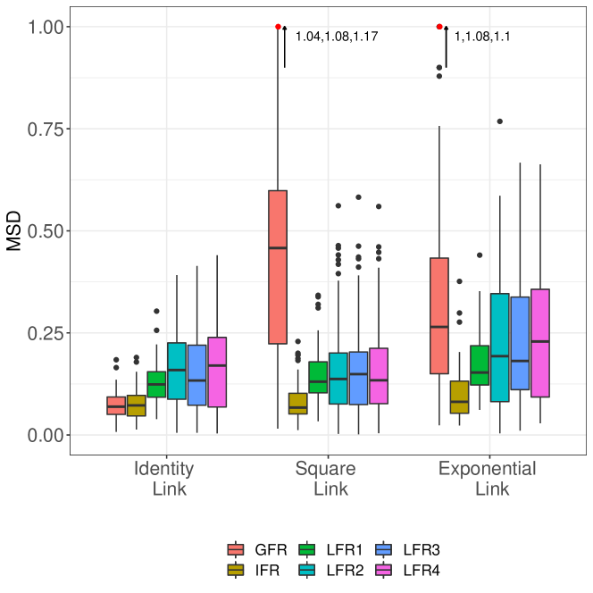
(a) Simulation Setting I.

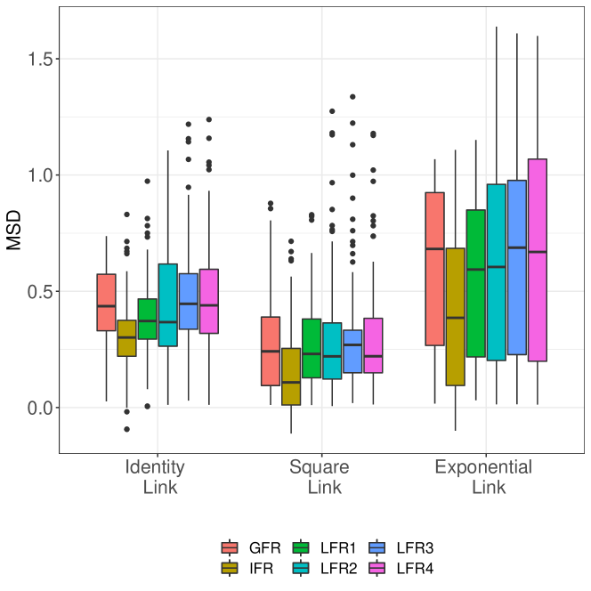
(b) Simulation Setting II.

Figure 1: Boxplot of the mean squared deviation (MSD) of the fits using the single index Fréchet regression model (IFR), the Global Fréchet regression (GFR) model, and four Local Fréchet Regression (LFR) models using the univariate predictor components, for sample size $n=1000.$ Left and right panels correspond to simulation settings I and II, respectively. The left, middle, and right columns in each of the panels correspond to the three different link functions used in the data generation mechanism, namely, identity, square, and exponential link functions, respectively; in all scenarios, the link functions are estimated from the data. In the left panel, the outliers having MSD greater than $1$ are marked in red with an upward arrow and the corresponding MSD values are overlaid.

Figure 2 demonstrates the effect of the index values on the distributional objects under simulation setting I for the different link functions when responses are represented in the form od densities. The three data generation mechanisms are shown in the left, middle, and right panels of Figure 2 respectively. For each case, the IFR model was fitted at the mean and mean$\pm 2$ sigma levels of the index values, displayed in red, blue, and green lines respectively, while the observed/simulated densities are overlaid in orange in each panel. In each case, for a higher value of the index level, the fitted densities shift towards the top-right, indicating a positive association of the single-index values on the mode of the distributions.

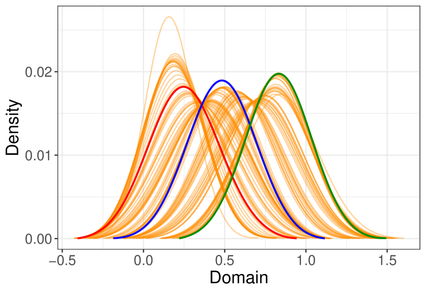
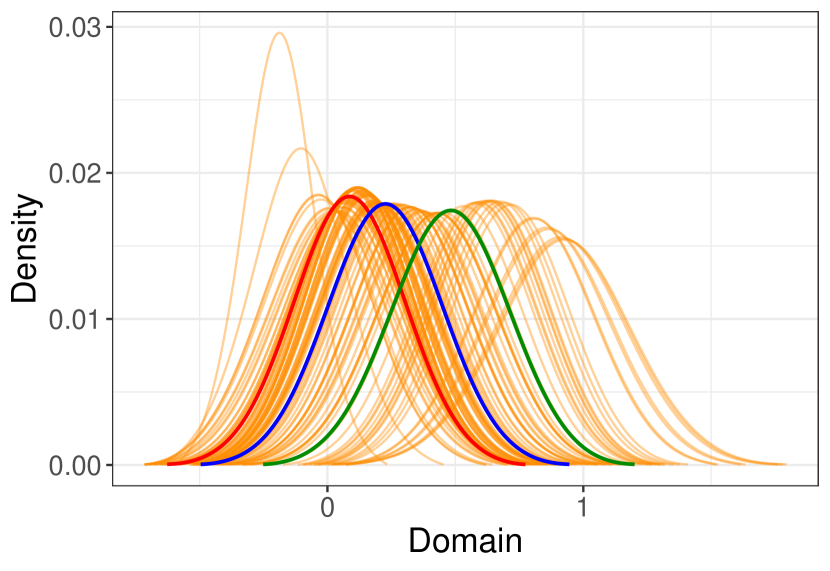
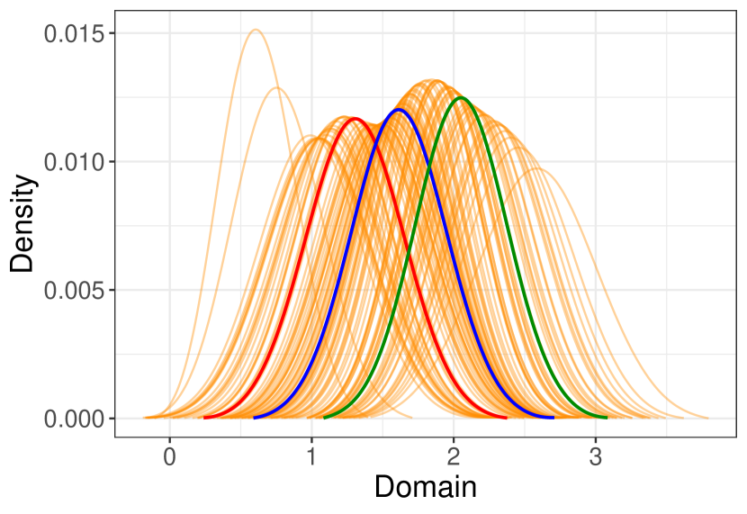
Figure 2: Simulated (orange) and fitted (red, blue, and green) distributional objects represented as densities for simulation setting I for sample size $n=1000.$ The left, middle, and right panels correspond to three link functions (identity, square, and exponential link) used in the data generation process. In each case, the IFR model fits are obtained at three different levels of the estimated index values, namely, at $t=$ mean$(\textbf{x}^{\top}\bm{\widehat{\widebar{\theta}}})-2\times$ sd($\textbf{x}^{\top}\bm{\widehat{\widebar{\theta}}}$) (red), $t=$ mean($\textbf{x}^{\top}\bm{\widehat{\widebar{\theta}}}$) (blue) and $t=$ mean$(\textbf{x}^{\top}\bm{\widehat{\widebar{\theta}}})+2\times$ sd($\textbf{x}^{\top}\bm{\widehat{\widebar{\theta}}}$) (green).

To illustrate the out-of-sample prediction performance of the proposed IFR model, the dataset was randomly split into a training set with sample size $n_{\text{train}}=\lfloor 2*n/3\rfloor$ and a test set with the remaining $n_{\text{test}}=n-\lfloor 2*n/3\rfloor$ subjects. The IFR method was implemented as follows: for any given unit direction $\bm{\bar{\theta}}\in\bar{\Theta},$ we partition the domain of the projections into $M$ equal-width non-overlapping bins and consider the representative observations $\tilde{\textbf{X}}_{l}$ and $\tilde{Y}_{l}$ for the data points belonging to the $l-$th bin. The “true” index parameter was estimated as $\bm{\widehat{\widebar{\theta}}}$ as per (12). We then took the fitted index obtained from the training set and predicted the responses in the test set using the covariates present in the test set. As a measure of the efficacy of the fitted model, we computed the root mean squared prediction error (RMPE) as

RMPE $$=\left[\frac{1}{M_{n_{\text{test}}}}\sum_{i=1}^{M_{n_{\text{test}}}}d_{W}^{2}\left(\tilde{Y}_{l}^{\text{test}},\hat{m}_{\oplus}(\tilde{\mathbf{X}}_{l}^{\text{test}\intercal}\bm{\widehat{\widebar{\theta}}},\bm{\widehat{\widebar{\theta}}})\right)\right]^{1/2},$$ (28)

where $\tilde{Y}_{l}^{\text{test}}$ and $\hat{m}_{\oplus}(\tilde{\mathbf{X}}_{l}^{\text{test}\intercal}\bm{\widehat{\widebar{\theta}}},\bm{\widehat{\widebar{\theta}}})$ denote, respectively, the $l^{\text{th}}$ observed and predicted responses in the test set, evaluated at the binned observation $\tilde{\mathbf{X}}_{l}^{\text{test}}$ and $d_{W}$ denotes the Wasserstein-2 metric in (S.3.1. Human mortality and age-at-death distributional object responses). We repeated this process $500$ times and computed RMPE for each split for the subjects separately. The mean and sd of the RMPE over the repetitions are shown in Table 3. The IFR model is seen to fare best across the different models and scenarios.

Table 3: Mean and sd (in parenthesis) of the RMPE as given in (B.50) comparing the performance of various Fréchet regression models: Index Fréchet Regression (IFR), Global Fréchet Regression (GFR), Local Fréchet Regression (LFR). The LFR fits are obtained for four individual predictor components separately.

	Setting I			Setting II
	Identity link	Square link	Exponential link	Identity link	Square link	Exponential link
IFR	0.0023 (0.0012)	0.0092 (0.0276)	0.0302 (0.0979)	0.0490 (0.0330)	0.1452 (0.0286)	0.1666 (0.0988)
GFR	0.0136 (0.0002)	0.1668 (0.0085)	0.1599 (0.0176)	0.0661 (0.0189)	0.2531 (0.0095)	0.3413 (0.0186)
LFR1	0.0478 (0.0014)	0.1671 (0.0084)	0.3516 (0.0299)	0.0679 (0.0191)	0.1317 (0.0096)	0.2371 (0.0310)
LFR2	0.0479 (0.0015)	0.1667 (0.0081)	0.3507 (0.0294)	0.0563 (0.0190)	0.1666 (0.0091)	0.1881 (0.0302)
LFR3	0.0476 (0.0020)	0.1684 (0.0133)	0.3468 (0.0296)	0.1218 (0.0191)	0.1992 (0.0142)	0.1812 (0.0304)
LFR4	0.0454 (0.0062)	0.1659 (0.0101)	0.3346 (0.0284)	0.0880 (0.0189)	0.2177 (0.0110)	0.2033 (0.0293)

For the case of distributional objects, the linear hypothesis test of $H_{0}$ in (22) against the sequence of alternatives $H_{1\delta}$ in (23) was also carried out. The power functions corresponding to the two simulation settings are shown in Figure 3(a) and  3(b), respectively. As $\delta$ increases, the power is seen to increase rapidly. This shows that the proposed test has non-trivial power (see Figure 3). When $\delta$ is close to $0,$ the test sizes are approximately equal to the nominal significance level of $\alpha=0.05.$ As expected, power increases with increasing sample size, most notably under the identity link. In the second simulation setting when the distributional objects are obtained by transporting a normal distribution, the power function increases at a slower rate, especially under the highly nonlinear (exponential) link function.

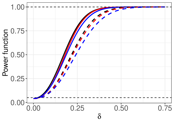
(a) Simulation Setting I.

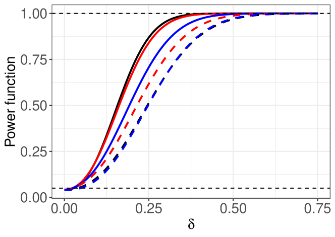
(b) Simulation Setting II.

Figure 3: Empirical power as function of $\delta$ for density object responses. The black, red, and blue curves correspond to the identity, square, and exponential link functions used in the data-generating mechanism, respectively, while the dashed and solid lines correspond to sample sizes $n=100$ and $n=1000$ respectively. The level of the tests is $\alpha=0.05$ and is indicated by the dashed line parallel to the x-axis.

4.2 Adjacency Matrices as Responses

These were generated for weighted graphs as random object responses; details are in Subsection LABEL:suppl:sec:adj of the Supplement.

4.3 Euclidean Responses

We applied the new approach targeting general random objects as responses for the special case of Euclidean responses. It is not specifically designed for this case, where targeted, well-studied and well-honed single index models have a long history. The numerical results show that the proposed method yields results that are somewhat inferior but overall still comparable to those obtained with specially tailored traditional single index approaches; see Subsection S.4.4 of the Supplement.

5 Data analysis

5.1 Resting state functional Magnetic Resonance Imaging: ADNI data

Resting-state functional Magnetic Resonance Imaging (fMRI) methodology makes it possible to study brain activation and to identify brain regions or cortical hubs that exhibit similar activity when subjects are in the resting state (Allen et al.,, 2014; Ferreira and Busatto,, 2013). In resting state fMRI, time series of Blood Oxygen Level Dependent (BOLD) signals are observed in regions of interest (ROI), where each ROI is represented by the signal of a seed voxel, which is the voxel in an ROI that has the highest correlation with the signals of nearby voxels. Alzheimer’s Disease has been found to be associated with anomalies in the functional integration of ROIs (Damoiseaux et al.,, 2012; Zhang et al.,, 2010).

Data used in the preparation of this article were obtained from the Alzheimer’s Disease Neuroimaging Initiative (ADNI) database (adni.loni.usc.edu). BOLD signals for $V=11$ brain seed voxels for each subject were extracted for the following ROIs: MPFC (Anterior medial prefrontal cortex), PCC (Posterior cingulate cortex), dMFPC (Dorsal medial prefrontal cortex), TPJ (Temporal parietal junction), LTC (Lateral temporal cortex), TempP (Temporal pole), vMFPC (Ventral medial prefrontal cortex), pIPL (Posterior inferior parietal lobule), Rsp (Retrosplenial cortex), PHC (Parahippocampal cortex) and HF⁺ (Hippocampal formation) (Andrews-Hanna et al.,, 2010). The pre-processing of the BOLD signals was implemented by adopting standard procedures of slice-timing correction, head motion correction and other standard steps. The signals for each subject were recorded over the interval $[0,270]$ (in seconds), with $K=136$ measurements available at two-second intervals. From this the temporal correlations were computed to construct the connectivity correlation matrix, also referred to as the Pearson correlation matrix in the neuroimaging community.

The data set in our analysis consists of $n=830$ subjects at four stages of the disease: $372$ CN (cognitively normal), $113$ EMCI (early mild cognitive impairment), $200$ LMCI (late mild cognitive impairment), and $145$ AD (Alzheimer’s) subjects. The inter-hub connectivity Pearson correlation matrix for the $i-th$ subject $Y_{i}$ with elements

$$(Y_{i})_{qr}=\frac{\sum_{p=1}^{K}(s_{ipq}-\bar{s}_{iq})(s_{ipr}-\bar{s}_{ir})}{\left[\left(\sum_{p=1}^{K}(s_{ipq}-\bar{s}_{iq})^{2}\right)\left(\sum_{p=1}^{K}(s_{ipq}-\bar{s}_{iq})^{2}\right)\right]^{1/2}},\,\,q,r=1,\dots,11$$ (29)

is the response object for each subject, where $s_{ipq}$ is the $(p,q)^{\text{th}}$ element of the signal matrix for the $i^{\text{th}}$ subject and $\bar{s}_{iq}:=\frac{1}{K}\sum_{p=1}^{K}s_{ipq}$ is the mean signal strength for the $q^{\text{th}}$ voxel. For Alzheimer’s disease studies, the ADAS-Cog-13 score (henceforth referred to as C score) is a widely-used measure of cognitive performance. It quantifies impairments across cognitive domains that are affected by Alzheimer’s disease (Kueper et al.,, 2018); higher scores indicate more serious cognitive deficiency.

We considered $p=10$ predictors, namely, $X_{1}=$ stage for the disease (coded as 0-3, indicating Cognitive normal (CN), Early and Late Mild cognitive impairment (EMCI and LMCI), or Alzheimer’s Disease (AD), respectively), $X_{2}=$ age of the subject (in years), $X_{3}=0$ is the subject is female and $=1$ if male), $X_{4}=$C score for the subject at the time of the first scan, and additionally all pairwise interaction terms between the above predictors, i.e., the products $X_{j}X_{k},\,j\neq k,1\leq j,k\leq 4$

In a first step, we test the null hypothesis of no regression effect, i.e., with $p=5$,

$$H_{0}:\bm{\theta_{0}}=\mathbf{0}_{(p-1)\times 1}\ vs.\ H_{1}:\text{ not all }\theta_{0j}\text{ are }0,\ j=2,\dots,p,$$

where ${\bm{\bar{\theta}_{0}}}=(\theta_{01},\bm{\theta_{0}})^{\top}$ and $\bm{\theta_{0}}=(\theta_{02},\dots,\theta_{0p})^{\top}$ with $\theta_{01}=\sqrt{1-\|\bm{\theta_{0}}\|^{2}}.$ The null model has $X_{1}$ included with $\theta_{01}=1$ since it is known that the stage of cognitive impairment has an effect on brain connectivity/ We obtain an estimate of the $(p-1)-$ dimensional vector $\hat{\bm{\theta}}$ as the minimizer of $V_{n}(\bm{\theta})$ as per (16) and $\hat{\theta}_{01}=\sqrt{1-\|\hat{\bm{\theta}}\|^{2}}.$ Under the null hypothesis, $\tilde{T}_{n}=\hat{\bm{\theta}}^{\top}(\widehat{\Lambda}^{\ast}_{B})^{-1}\hat{\bm{\theta}}\overset{approx.}{\sim}\chi^{2}_{(p-1)}.$ We find that $\tilde{T}_{n}=23.81$, corresponding to a $p$ value of $p=0.0046<0.005,$ providing evidence that there is indeed a regression relationship.

Table 4: Details on step-wise model selection.

	Step 1		Step 2		Step 3
	Coeff.	p-value	Coeff.	p-value	Coeff	p-value
Age	-0.364	0.005	-0.394	-	-0.401	-
Gender	0.198	0.122	0.558	0.161	0.173	0.113
C Score	0.371	0.094	0.207	0.010	0.279	-

We also implemented sequential predictor selection, where we specified an “alpha-to-enter” level $\alpha=0.05$ and considered $X_{1}$ to be in the model and included each of $X_{2},$ $X_{3},$ and $X_{4}$ in the model separately along with $X_{1}$ then testing the null hypotheses $\theta_{j}=0,\ j=2,3,4$ separately. Table 4 illustrates the resulting step-wise model selection.

For example, for testing $\theta_{2}=0$, we first obtained $\hat{\theta}_{2}=-0.364$, $\hat{\theta}_{1}=\sqrt{1-(-.364)^{2}}=0.931$) and $\tilde{T}_{n}=7.88$ with a $p$-value of $0.005.$ Thus $X_{2}$ (age) was added to the model in step 1, followed by adding $X_{4}$ (C score) in step 2, while $X_{3}$ (gender) was not significant. With $X_{1},$ $X_{2},$ and $X_{4}$ in the model, we tested for the significance of the pairwise interaction terms. The null hypothesis for this test is $H_{0}:\theta_{5}=\theta_{6}=\dots=\theta_{10}=0.$ The p-value was $0.106,$ and we did not include interactions in the final model. The estimated average Fréchet error $\frac{1}{n}\sum_{i=1}^{n}d^{2}(Y_{i},\hat{m}_{\oplus}(X_{1i}\hat{\theta}_{1}+X_{2i}\hat{\theta}_{2}+X_{4i}\hat{\theta}_{4}))$ was quite small $(0.239).$

To construct the confidence regions for the coefficients $(\theta_{1},\theta_{2},\theta_{4})$, we implemented the local linear Fréchet regression with the Epanechnikov kernel and used 5-fold cross-validation to select the bandwidth $b$. Using the bootstrap method to obtain the estimated covariance matrix of the limiting distribution we obtained the $95\%$ pairwise confidence ellipses for the coefficients $(\theta_{1},\theta_{2},\theta_{4})$ of the predictors- disease stage, age, and C score, which are displayed in Figure 4. We observe that none of the pairwise confidence ellipses includes the origin and therefore the p-values are $<0.05,$ implying the significance of the predictors.

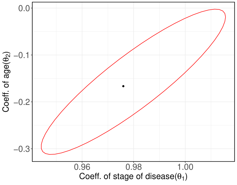
(a) Confidence ellipse for $(\theta_{1},\theta_{2}).$

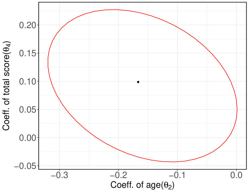
(b) Confidence ellipse for $(\theta_{2},\theta_{4}).$

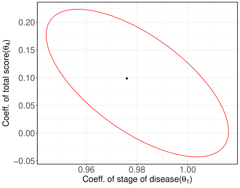
(c) Confidence ellipse for $(\theta_{1},\theta_{4}).$

Figure 4: The $95\%$ confidence ellipses for pairs of coefficients for predictors stage of the disease ($X_{1}$), age ($X_{2}$), and C score ($X_{4}$).

To illustrate the effect of the single index on the response, we computed the estimated index of the fitted model for each subject and then obtained the $25\%,50\%,$ and $75\%$ quantiles across all subjects, with values $q_{1}=15.048,$ $q_{2}=16.430$ and $q_{3}=18.250,$ respectively. The values of the four covariates for the subjects with estimated index values closest to $q_{1},$ $q_{2},$ and $q_{3}$ are in Table 5, and their observed and fitted functional connectivity correlation matrices are illustrated in Figure 5. The fitted correlation matrices correspond to the values of the estimated object link function at the three index values and are contrasted with the observed correlation matrices for the three subjects. This gives an idea of how the fitted correlation matrix changes as the index move through the three quantile levels.

Table 5: Covariate values for the subjects with estimated index values closest to the first three quantiles of the estimated index when considered across all subjects, $q_{1}(15.048),$ $q_{2}(16.430),$ and $q_{3}(18.250),$ respectively. Subject $726$ has an estimated index value that is closest to $q_{1}$, subject 695 closest to $q_{2}$, and subject 556 closest to $q_{3}.$

Subject number	Estd. index value	Stage of the disease	Age	Gender	C score
726	15.045	2	66.10 y	M	20.33
695	16.430	2	78.12 y	M	14
556	18.252	1	72.55 y	M	51.67

We observe that the fits match the general pattern of the observed matrices quite well. The Frobenius distances between the observed and the estimated matrices at $q_{1},$ $q_{2},$ and $q_{3}$ are $1.68,$ $1.10,$ and $0.79,$ respectively. The fitted model reflects the trends seen in the observed correlation matrices and illustrates the nonlinear dependence of functional connectivity on the index value.

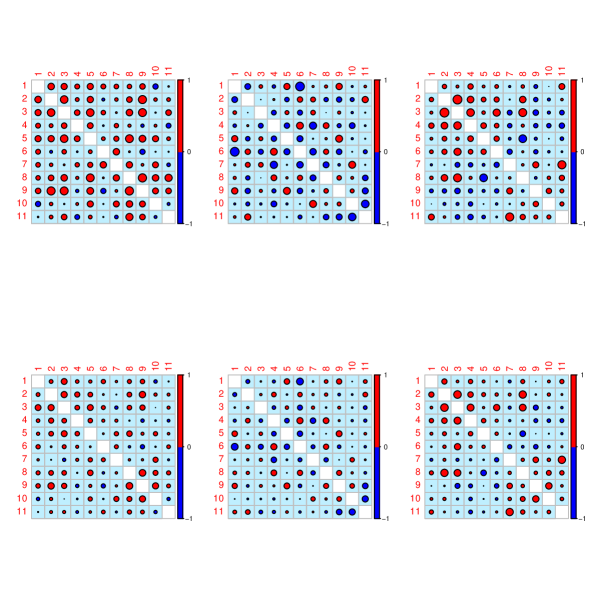
Figure 5: Observed and fitted functional connectivity correlation matrices for different values of the single index. The panels in the top row, from left to right, depict the observed functional connectivity correlation matrices for those subjects for whom the estimated index values are closest to the $25\%,50\%,$ and $75\%$ quantile of all indices across subjects, respectively. The bottom row shows the fitted functional connectivity correlation matrices for the same subjects, (from left to right). Positive (negative) values for correlations are drawn in red (blue), where larger circles correspond to larger absolute values.

We also studied the out-of-sample prediction performance of the proposed IFR model, for which we used the root mean squared prediction error

$$\text{RMPE}=\left[\frac{1}{M_{n_{\text{test}}}}\sum_{i=1}^{M_{n_{\text{test}}}}d_{F}^{2}\left(\tilde{Y}_{l}^{\text{test}},\hat{m}_{\oplus}(\tilde{\textbf{X}}_{l}^{\top}\bm{\widehat{\widebar{\theta}}},\bm{\widehat{\widebar{\theta}}})\right)\right]^{1/2},$$ (30)

where $\tilde{Y}_{l}^{\text{test}}$ and $\hat{m}_{\oplus}(\tilde{\textbf{X}}_{l}^{\top}\bm{\widehat{\widebar{\theta}}})$ denote, respectively, the $l^{\text{th}}$ observed and predicted responses in the test set, evaluated at the binned observation $\tilde{\textbf{X}}_{l}.$ Here, $n_{\text{train}}$ and $n_{\text{test}}$ denote the sample sizes of the training and testing sets formed by randomly splitting the data. We repeated this process $200$ times, and computed RMPE for each split for the subjects separately. The tuning parameters $(b,M)$ were chosen by a $5-$fold cross-validation method for each replication of the process. The prediction performance of the IFR model was compared with other applicable Fréchet regression models, namely, the global Fréchet regression (GFR) model with the three-dimensional predictor $(X1,X_{2},X_{4})$ and two separate local linear Fréchet regression (LFR) models, one with the single predictor $X_{2}$ (age) and the other with the single predictor $X_{4}$ (C score). When comparing the performance of these models (Table 6), we find

Table 6: Mean and sd (in parenthesis) of the root mean prediction error (RMPE) over $200$ Monte Carlo simulation runs for various object regression methods. The methods compared are index Fréchet regression (IFR); global Fréchet Regression (GFR) with the three predictors stage of the disease, age, and ADSA score; and two local linear Fréchet regression (LFR) models with separate one-dimensional predictors.

IFR	GFR	LFR1 (Predictor Age)	LFR2 (Predictor C Score)
0.3066 (0.012)	0.5083 (0.011)	0.5076 (0.012)	0.5326 (0.013)

that the out-of-sample prediction error is low for the IFR model, as compared to the global and local Fréchet regression approaches. In fact, it is not far from the in-sample prediction error $(0.251)$, calculated as the average distance between the observed training sample and the predicted objects based on the covariates in the training sets. This motivates the proposed IFR models.

5.2 Human mortality data: Age-at-death distributions as responses

Lifetables reflecting human mortality across 40 countries correspond to distributional responses, coupled with various country-specific covariates. We implement an overall test for the regression effect for these data. Details about this analysis are in the Supplement, subsection S.4.1.

5.3 Emotional well-being of unemployed workers: Compositional data as responses.

We further demonstrate the proposed IFR method for the analysis of mood compositional data. Here the object-valued responses lie on a manifold (sphere) with positive curvature. Thus the sufficient (but not necessary) condition for assumption (A5) that the underlying metric space behaves like a CAT(0) space is not satisfied, however, the numerical performance of the IFR method remains quite good; see Supplement, subsection S.4.2. This suggests a certain degree of model robustness.

6 Discussion

Binning the data to reduce the effective sample size is not necessary for the basic consistency results without rates. As discussed at the end of Section 2, the binning method is introduced in order to invoke the uniform consistency rate for the local Fréchet regression and the effective sample size $M=M(n)$ is tied to this rate by virtue of assumption 14. To avoid confusion, we discuss the binning approach throughout. The rate of convergence for $\bm{\widehat{\widebar{\theta}}}-{\bm{\bar{\theta}_{0}}}$ is $M^{-1/2}$. Since our rate results and proofs rely on the uniform convergence rate of local Fréchet regression, this rate cannot be improved within the current framework and overcoming these limits would require a fundamentally different approach.

The assumptions required to obtain the technical results are essentially the same as those used before in the Fréchet regression literature, specifically in Chen and Müller, (2022). We require curvature and entropy conditions to hold uniformly across all index values and direction parameters. The curvature and entropy conditions can be verified for commonly observed objects such as univariate probability distributions, positive definite matrices, or data on the surface of a sphere, as well as other random objects under suitable metrics. The Lipschitz condition (A2) on the link function is standard in single-index models, while assumption (A5) reflects the interplay between the properties of the metric and the link function. Assumption (A5) is implied by the easier-to-interpret assumption (K1)-(K3) (see Appendix Appendix B).

The classical single index model for Euclidean responses has been recently extended to a single index coefficient model for quantile regression (Zhao et al.,, 2017). This is a desirable extension for the object case of index Fréchet regression as well. One problem to resolve in this case is to define quantiles in the metric space where the object responses lie since there is no order. The problem of defining quantiles is already difficult and ambiguous for multivariate Euclidean objects. This is a potentially interesting topic for future research.

Finally, inference results for object regression are scarce. For example, the Wasserstein $F$-tests proposed by Petersen et al., (2021) are exclusively aimed at univariate distribution quantiles within the specific setting of global Fréchet regression. We provide here a general framework to obtain inference for the case of vector predictors coupled with object responses, which includes generalized versions of inference for model comparisons and for assessing the significance of individual predictors.

*equationsection *thmsection *lemsection *corsection

Appendix Appendix A Geodesics and curvature

The length of a curve $\phi:[0,1]\to\Omega$ connecting two distinct points $x,y\in\Omega$ can be measured by taking partitions $P=\{t_{0}\leq t_{1}\leq\cdots\leq t_{k}\}\subset[0,1]$ and finding the supremum polygonal length

$$|\phi|:=\sup_{P\in\mathcal{P}}\sum_{j=1}^{k}d(\phi(t_{j}),\phi(t_{j-1})),$$

where $\mathcal{P}$ is any collection of subsets of $[0,1]$ with finite cardinality. The metric space $(\Omega,d)$ is a length space if $d(x,y)=\inf_{\phi}|\phi|$, where the infimum ranges over all curves $\phi:[0,1]\to\Omega$ connecting two distinct points $x$ and $y$, that is, i.e., $\phi(0)=x$ and $\phi(1)=y$. A geodesic on $\Omega$ connecting two distinct points $x$ and $y$ is the shortest path connecting the two points. Geodesics in a metric space are analogous to straight lines in a Euclidean space.

Unlike Euclidean spaces, a general metric space may not be flat, and curvature is used to measure the amount of deviation from being flat. The curvature of a given geodesic space is classified by comparing the geodesic triangles on the metric space to those on the corresponding reference spaces $M_{\kappa}^{2}.$ When $\kappa=0$, $M_{\kappa}^{2}=\mathbb{R}^{2}$ with the standard Euclidean distance $d_{E}(x,y)=||x-y||_{E},$ for any $x,y\in\mathbb{R}^{2}.$ A geodesic triangle with vertices $p,q,r$ in a geodesic space $\Omega$, denoted by $\triangle(p,q,r)$, consists of three geodesic segments that connect $p$ to $q$, $p$ to $r$ and $q$ to $r$, respectively. A comparison triangle $\triangle(\bar{p},\bar{q},\bar{r})$ in the reference space $M_{k}^{2}=\mathbb{R}^{2}$ is a geodesic triangle in $\mathbb{R}^{2}$ formed by the vertices $\bar{p},$ $\bar{q},$ and $\bar{r}$ such that,

$$d(p,q)=||\bar{p}-\bar{q}||_{E},\ d(q,r)=||\bar{q}-\bar{r}||_{E},\ d(p,r)=||\bar{p}-\bar{r}||_{E}.$$ (A.31)

$\Omega$ is said to have a non-positive curvature if there exists a comparison triangle $\triangle(\bar{p},\bar{q},\bar{r})$ in the reference space $\mathbb{R}^{2}$ such that $d(x,y)\leq||\bar{x}-\bar{y}||_{E}$ for all $x\in\overline{pq}$ and $y\in\overline{pr}$ and their comparison points $\bar{x}$ and $\bar{y}$ on $\triangle(\bar{p},\bar{q},\bar{r})$. A geodesic space with curvature upper bounded by $0,$ in which every geodesic triangle $\triangle(p,q,r)$ satisfies the following $\mathrm{CAT}(0)$ inequality is a CAT(0) space,

$$d(x,y)\leq||\bar{x}-\bar{y}||_{E}\text{ for all }x\in\overline{pq}\text{ and }y\in\overline{pr}\text{ and their comparison points }\bar{x},\bar{y}\in\mathbb{R}^{2}.$$ (A.32)

Every CAT(0) space is uniquely geodesic. Examples of CAT(0) spaces include Euclidean space, the space of symmetric positive definite matrices, Wasserstein-2 spaces, or phylogenetic tree spaces. For a detailed introduction to metric geometry, we refer to Burago et al., (2001). A compilation of the most relevant facts can be found in Lin and Müller, (2019).

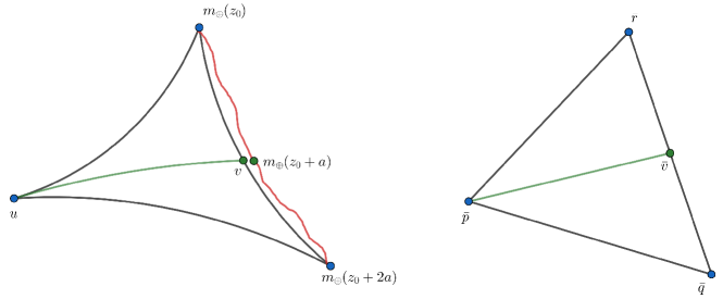
Figure A.6: Left figure: Geodesic triangle formed by the three points $u,$ $m_{\oplus}(z_{0}),$ $m_{\oplus}(z_{0}+2a)$, where $v$ is the midpoint of the geodesic connecting the points $m_{\oplus}(z_{0})$ and $m_{\oplus}(z_{0}+2a).$ The red line depicts the true regression function $m_{\oplus}.$ $m_{\oplus}(z_{0}+a)$ is closely approximated by $v$ lying on a geodesic that connects $m_{\oplus}(z_{0})$ with $m_{\oplus}(z_{0}+2a).$ Right figure: Reference triangle in $\mathbb{R}^{2}$ as an illustration of the CAT(0) inequality.

Appendix Appendix B Sufficient conditions for assumption (A5)

We discuss here sufficient conditions under which assumption (A5) holds. For this we consider the following assumptions:

1. $(\Omega,d)$ is a CAT(0) space, that is every geodesic triangle satisfies the CAT(0) inequality in (A.32).

For any $z_{0}\in\mathbb{R},$ and $u\in\Omega,$ there exists some $a_{0}>0,$ such that for small enough $a\in(0,a_{0}],$ we may consider the geodesic triangle formed by $u,$ $m_{\oplus}(z_{0}),$ $m_{\oplus}(z_{0}+2a)$ for $z_{0},z_{0}+2a\in\mathcal{T},$ for which we assume the following.

1. Defining the midpoint $v$ of the geodesic path connecting $m_{\oplus}(z_{0})$ and $m_{\oplus}(z_{0}+2a)$ such that

   $$d(m_{\oplus}(z_{0}),v)=d(m_{\oplus}(z_{0}+2a),v)=\frac{1}{2}d(m_{\oplus}(z_{0}+2a),m_{\oplus}(z_{0})),$$ (B.33)

   we require

   $$d(m_{\oplus}(z_{0}+a),v)\leq C_{\ast}a^{2},$$ (B.34)

   where $C_{\ast}>0$ does not depend on $z_{0},$ and is such that, $L_{\ast}^{2}>2DC_{\ast},$ $L_{\ast}$ and $D$ being the lower Lipschitz constant for $m_{\oplus}$ from assumption (A2), and the diameter of the metric space $\Omega,$ respectively.

2. There exist real constants $L_{\ast}>0$ such that, for all x with norm bounded both above and below, and for all $\bm{\bar{\theta}}_{1},\bm{\bar{\theta}}_{2}\in\bar{\Theta},$

   $$d\left(m_{\oplus}(\textbf{x}^{\top}\bm{\bar{\theta}}_{1},\bm{\bar{\theta}}_{1}),m_{\oplus}(\textbf{x}^{\top}\bm{\bar{\theta}}_{2},\bm{\bar{\theta}}_{2})\right)\geq L_{\ast}\|\bm{\bar{\theta}}_{1}-\bm{\bar{\theta}}_{2}\|.$$

Figure B.7 illustrates the geometry of the geodesic triangles in $\Omega$ and its reference space $\mathbb{R}^{2}.$ Assumption (K2) can be verified when the link function $m_{\oplus}$ is smooth enough for the case of conventional Euclidean single index models. It thus provides an extension of the usual smoothness assumption in the case of random object responses. In section C of the Supplement We discuss this further in the context of Euclidean responses and in the case where the responses lie in the space of distributions equipped with Wasserstein-2 metric, and derive assumption (A5) under the sufficient conditions (K1), (K2), and (K3).

Assumption (K3) in conjunction with assumption (A2) implies that the link function $m_{\oplus}$ is bi-Lipschitz. This limits the rate at which the object $m_{\oplus}$ can change, essentially it cannot change too fast or too slowly. A bi-Lipschitz function is an injective Lipschitz function whose inverse function is also Lipschitz. The bi-Lipschitz condition is stronger than the common assumption of a monotone link function in classical single index modeling with Euclidean responses. In the special case of $\Omega=\mathbb{R}$ this reduces to requiring a monotone differentiable function with strictly positive derivative almost everywhere and restricts the monotonicity to a smaller subclass of strictly monotone functions. In the special case of Euclidean responses, this simplifies to the assumption that the link function $m_{\oplus}=m$ is monotone and differentiable such that $m^{\prime}(x)$ is strictly monotone with continuous derivative bounded away from zero. Such technical assumptions are commonly used for deriving distributional results in the existing single index literature, by virtue of a Taylor expansion of the link function $m$ in the Euclidean case.

Supplementary Material

S.1. Technical assumptions (U1)- (U3), (R1)- (R2)

In this section, we describe the technical assumptions needed to establish the uniform rate of convergence for the local linear Fréchet regression estimator in Lemma 1 in Section 3 of the main manuscript. We also provide motivation and discuss suitable examples regarding the assumptions.

The assumptions required to obtain the technical results are essentially the same as those used before in the Fréchet regression literature, specifically in Chen and Müller, (2022). To adapt these assumptions to the present situation, we require the curvature and entropy conditions to hold uniformly across all index values and direction parameters. The curvature and entropy conditions can be verified for commonly observed objects such as univariate probability distributions, positive definite matrices, or data on the surface of a sphere, as well as other random objects under suitable metrics.

Denote by $\mathcal{T}_{\bm{\bar{\theta}}}$ the support of the random variable $T=\textbf{X}^{\top}\bm{\bar{\theta}}$ for any given unit direction $\bm{\bar{\theta}}\in\bar{\Theta},$ where $\bar{\Theta}$ is defined in equation (2.5) of the main manuscript. Under assumption (A3), for bounded random variables $\textbf{X},$ we can write $\mathcal{T}_{\bm{\bar{\theta}}}\subset\mathcal{T}$ for some bounded subset $\mathcal{T}$ of $\mathbb{R}.$ For a given direction $\bm{\bar{\theta}}\in\bar{\Theta}$ such that $\textbf{X}^{\top}\bm{\bar{\theta}}=t,$ where $\bar{\Theta}$ is as given in equation (2.5), the conditional Fréchet mean is given by

$$m_{\oplus}(t,\bm{\bar{\theta}})=\underset{\omega\ \in\ \Omega}{\operatorname*{argmin}}\ M(\omega,t,\bm{\bar{\theta}});\quad M(\omega,t,\bm{\bar{\theta}}):=\mathbb{E}{(d^{2}(Y,\omega)|\textbf{X}^{\top}\bm{\bar{\theta}}=t)},$$ (B.35)

and the local linear Fréchet regression estimate by

$$\hat{m}_{\oplus}(t,\bm{\bar{\theta}})=\underset{\omega\ \in\ \Omega}{\operatorname*{argmin}}\ \hat{L}_{n}(\omega,t,\bm{\bar{\theta}});\quad\hat{L}_{n}(\omega,t,\bm{\bar{\theta}}):=\frac{1}{n}\sum_{i=1}^{n}\widehat{S}(\textbf{X}_{i}^{\top}\bm{\bar{\theta}},t,b)d^{2}(Y_{i},\omega)),$$ (B.36)

where $\widehat{S}$ is the empirical estimate (from equation (2.10)) of the nonparametric weight function (described in equation (2.8)) in Section 2 of the main manuscript and $b$ is the bandwidth parameter for the kernel involved in the localized Fréchet mean. We also define the intermediate localized weighted Fréchet means as

$$\tilde{m}_{\oplus}(t,\bm{\bar{\theta}})=\underset{\omega\ \in\ \Omega}{\operatorname*{argmin}}\ \tilde{L}_{b}(\omega,t,\bm{\bar{\theta}});\quad\tilde{L}_{b}(\omega,t,\bm{\bar{\theta}}):=\mathbb{E}{(S(\textbf{X}^{\top}\bm{\bar{\theta}},t,b)d^{2}(Y,\omega))},$$ (B.37)

where the nonparametric weight function is described in equation (2.8) in the main manuscript. The following additional assumptions are required, which are analogous versions of the assumptions in Chen and Müller, (2022).

1. For all $t\in\mathcal{T}$ and $\bm{\bar{\theta}}\in\bar{\Theta},$ the minimizers $m_{\oplus}(t,\bm{\bar{\theta}})$, $\hat{m}_{\oplus}(t,\bm{\bar{\theta}})$, and $\tilde{m}_{\oplus}(t,\bm{\bar{\theta}})$ exist and are unique, the latter two almost surely. In addition, for any $\varepsilon>0$,

   $$\begin{gathered}\inf_{t\in\mathcal{T}}\inf_{d(m_{\oplus}(t,\bm{\bar{\theta}}),\omega)>\varepsilon}[M(\omega,t,\bm{\bar{\theta}})-M(m_{\oplus}(t,\bm{\bar{\theta}}),t,\bm{\bar{\theta}})]>0,\\ \liminf_{b\to 0}\inf_{t\in\mathcal{T}}\inf_{d(\omega,\tilde{m}_{\oplus}(t,\bm{\bar{\theta}}))>\varepsilon}[\tilde{L}_{b}(\omega,t,\bm{\bar{\theta}})-\tilde{L}_{b}(\tilde{m}_{\oplus}(t,\bm{\bar{\theta}}),t,\bm{\bar{\theta}})]>0,\end{gathered}$$ (B.38)

   and there exists $c=c(\varepsilon)>0$ such that

   $$\begin{gathered}P\left(\inf_{t\in\mathcal{T}}\inf_{d(\hat{m}_{\oplus}(t,\bm{\bar{\theta}}),\omega)>\varepsilon}[\hat{L}_{n}(\omega,t,\bm{\bar{\theta}})-\hat{L}_{n}(\hat{m}_{\oplus}(t,\bm{\bar{\theta}}),t,\bm{\bar{\theta}})]\geq c\right)\to 1.\end{gathered}$$ (B.39)

2. Let $\mathcal{B}_{r}(m_{\oplus}(t,\bm{\bar{\theta}}))\subset\Omega$ be a ball of radius $r$ centered at $m_{\oplus}(t,\bm{\bar{\theta}})$ and
   $\mathcal{N}(\varepsilon,\mathcal{B}_{r}(m_{\oplus}(t,\bm{\bar{\theta}})),d)$ be its covering number using balls of radius $\epsilon.$ Then

   $$\begin{gathered}\underset{r\to 0+}{\lim}\int_{0}^{1}\sup_{t\in\mathcal{T}}\sqrt{1+\log\mathcal{N}(r\varepsilon,\mathcal{B}_{r}(m_{\oplus}(t,\bm{\bar{\theta}})),d)}d\epsilon=O(1).\end{gathered}$$ (B.40)

3. There exists $r_{1},r_{2}>0,$ $c_{1},c_{2}>0,$ and $\beta_{1},\beta_{2}>1$ such that

   $$\inf_{t\in\mathcal{T}}\ \inf_{d(m_{\oplus}(t,\bm{\bar{\theta}}),\omega)<r_{1}}[M(\omega,t,\bm{\bar{\theta}})-M(m_{\oplus}(t,\bm{\bar{\theta}}),t,\bm{\bar{\theta}})-c_{1}d^{2}(\omega,m_{\oplus}(t,\bm{\bar{\theta}}))^{\beta_{1}}]\geq 0,$$

   $$\underset{b\to 0}{\liminf}\ \inf_{t\in\mathcal{T}}\inf_{d(\omega,\tilde{m}_{\oplus}(t,\bm{\bar{\theta}}))<r_{2}}\ [\tilde{L}_{b}(\omega,t,\bm{\bar{\theta}})-\tilde{L}_{b}(d(\tilde{m}_{\oplus}(t,\bm{\bar{\theta}}),t,\bm{\bar{\theta}})-c_{2}d^{2}(\omega,\tilde{m}_{\oplus}(t,\bm{\bar{\theta}}))^{\beta_{2}}]\geq 0.$$ (B.41)

Furthermore, we require the following assumptions for kernels and distributions.

1. The kernel $K$ is a probability density function, symmetric around zero, uniformly continuous on $\mathbb{R}$ such that $\int_{\mathbb{R}}K(x)^{j}x^{k}<\infty,$ for $j,k=1,\dots 6.$ The derivative $K^{\prime}$ exists and is bounded on the support of $K$, i.e., $\sup_{x:K(x)>0}|K^{\prime}(x)|<\infty.$ Additionally, $\int_{\mathbb{R}}x^{2}|K^{\prime}(x)|\sqrt{|x\log|x||}dx<\infty.$

2. For any given unit direction $\bm{\bar{\theta}}\in\bar{\Theta},$ the marginal density $f_{T,\bm{\bar{\theta}}}$ of $T=\textbf{X}^{\top}\bm{\bar{\theta}}$ and the conditional densities $f_{T,\bm{\bar{\theta}}|Y}(\cdot,y)$ of $T$ given $Y=y$ exist and are twice continuously differentiable in the interior of $\mathcal{T}$ for all $\bm{\bar{\theta}}\in\bar{\Theta}$, the latter for all $y\in\Omega$. The marginal density $f_{T,\bm{\theta}}$ is bounded away from zero on its support $\mathcal{T}$ for all $\bm{\bar{\theta}}\in\bar{\Theta}$ i.e., $\inf_{t\in\mathcal{T}}\ f_{\textbf{X}^{\top}\bm{\bar{\theta}}}(t)>0.$

   The second-order derivative $f_{T,\bm{\bar{\theta}}}^{\prime\prime}$ is uniformly bounded for all $t\in\mathcal{T},$ $\bm{\bar{\theta}}\in\bar{\Theta},$ that is,
   $\sup_{t\in\mathcal{T}}|f_{T,\bm{\bar{\theta}}}^{\prime\prime}(t)|<\infty$. The second-order partial derivatives $(\partial^{2}f_{T,\bm{\bar{\theta}}|Y}/\partial t^{2})(\cdot,y)$ are uniformly bounded, uniform over all $\bm{\bar{\theta}}\in\bar{\Theta}$, i.e.,
   $\sup_{t\in\mathcal{T}}\ \sup_{y\in\Omega}|(\partial^{2}f_{T,\bm{\bar{\theta}}|Y}/\partial t^{2})(\cdot,y)|<\infty.$

   Additionally, for any open set $B\subset\Omega$, $P(Y\in B|\textbf{X}^{\top}\bm{\theta}=t)$ is continuous as a function of $t$ and $\bm{\bar{\theta}}.$ For any $t\in\mathcal{T}$ and $\bm{\bar{\theta}}\in\bar{\Theta},$ $M(\omega,t,\bm{\bar{\theta}})$ is equicontinuous, that is,

   $$\limsup_{\bm{\bar{\theta}}_{1}\to\bm{\bar{\theta}}_{2}}\ \sup_{t\in\mathcal{T}}\ \sup_{\omega\in\Omega}\left|M(\omega,t,\bm{\bar{\theta}}_{1})-M(\omega,t,\bm{\bar{\theta}}_{2})\right|=0.$$

Similar yet weaker assumptions have been made in Petersen and Müller, (2019) for pointwise rates of convergence for local linear Fréchet regression estimators.  Chen and Müller, (2022) made stronger assumptions in this regard to establish uniform convergence results over univariate predictor values. In the above assumptions (U1)- (U3) we adapt those in Chen and Müller, (2022), incorporating uniform bounds over the index parameter as well as over the values of the single index. Since the objective function for the local Fréchet regression involves both the index value $\textbf{x}^{\top}\bm{\bar{\theta}}=t$ and the index parameter $\bm{\bar{\theta}}$, conditions on the well-separatedness, entropy, and curvature needs to be extended for all values of $t$ and $\bm{\bar{\theta}}.$ These assumptions are adapted from empirical process theory, guarantee the asymptotic uniform equicontinuity of $\tilde{L}_{b}$, and control the behavior of $\tilde{L}_{b}-M$ and $\hat{L}_{n}-\tilde{L}_{b}$ near the minimizers $m_{\oplus}(t,\bm{\bar{\theta}})$ and $\tilde{m}_{\oplus}(t,\bm{\bar{\theta}})$, respectively, uniformly over $t$ and $\bm{\bar{\theta}}.$ assumption (U1) is commonly used to establish the uniform consistency of M-estimators (Van der Vaart and Wellner,, 2000) by showing the weak convergence of the respective empirical processes. In conjunction with the assumption that the metric space $\Omega$ is totally bounded, this implies the pointwise convergence of the minimizers for any given $t$ and $\bm{\bar{\theta}}$; it also ensures that the asymptotic uniform equicontinuity of $\tilde{L}_{b}$ and $\hat{L}_{n}$, and implies the (asymptotic) uniform equicontinuity of $\tilde{m}_{\oplus}$ and $\hat{m}_{\oplus}$, whence the uniform convergence of the minimizers follows as the support of $\textbf{x}^{\top}\bm{\bar{\theta}}$ is compact for any $\bm{\bar{\theta}}$.

Assumptions (U1)- (U3) are easily verified for specific metric space-valued objects.

• Let $\Omega$ be the set of probability distributions on a closed interval of $\mathbb{R}$ with finite second moments, endowed with the Wasserstein-2 distance $d_{W}$, i.e., for any two distributional objects $Y_{1}$ and $Y_{2}$ with cdfs $F_{Y_{1}}$ and $F_{Y_{2}}$ respectively,

  $$d_{W}(Y_{1},Y_{2})=\int_{0}^{1}(F_{Y_{1}}^{-1}(z)-F_{Y_{2}}^{-1}(z))^{2}dz,$$

  where $F_{Y_{j}}^{-1}(z)$ is the quantile function for $Y_{j}$, $j=1,2.$ The Wasserstein space $(\Omega,d_{W})$ satisfies assumptions (U1)- (U3) with $\beta_{1}=\beta_{2}=2.$

• Let $\Omega$ be the space of $r$-dimensional correlation matrices, i.e., symmetric, positive semidefinite matrices in $\mathbb{R}^{r\times r}$ with diagonal elements equal to $1$, endowed with the Frobenius metric $d_{F}$ . Specifically for any two elements $Y_{1},Y_{2}\in\Omega$,

  $$d_{F}(Y_{1},Y_{2})=\sqrt{{\rm trace}{((Y_{1}-Y_{2})^{\intercal}(Y_{1}-Y_{2}))}}.$$

  The space $(\Omega,d_{F})$ satisfies assumptions (U1)- (U3) with $\beta_{1}=\beta_{2}=2.$

For Examples 1-2, we note that since the Wasserstein space for one-dimensional distributions and the space of correlation matrices are Hadamard spaces, there exists a unique minimizer of $M(\cdot,t,\bm{\bar{\theta}})$ for any $t\in\mathcal{T}$ and $\bm{\bar{\theta}}\in\bar{\Theta}$ (Sturm,, 2003). Examples 1-2 follow from similar arguments as those in the proofs of Propositions 1-2 of Petersen and Müller, (2019) by observing that the arguments hold uniformly across $t$ and $\bm{\bar{\theta}}.$ Assumptions (R1) and (R2) are standard distributional assumptions for local nonparametric regression and are needed to show the convergence of the bias and stochastic parts for the local linear Fréchet estimator uniformly over all $t$ and $\bm{\bar{\theta}}.$ In particular, Assumption (R1) can be verified for a general class of kernel functions given by

$$c_{\kappa}(1-x^{2})^{\kappa}\mathbb{I}\left([-1,1]\right),\ \kappa\in\mathcal{Z},$$

where $c_{\kappa}=\frac{\Gamma(k+\frac{3}{2})}{\sqrt{\pi}\Gamma(k+1)}$ is such that $\int_{-1}^{1}c_{\kappa}(1-x^{2})^{\kappa}dx=1$ and the indicator function is defined as $\mathbb{I}\left(A\right)=1\text{ if }\textbf{X}\in A,\text{ and }0\text{ otherwise.}$ The Epanechnikov kernel $K(x)=\frac{3}{4}(1-x^{2})\mathbb{I}\left([-1,1]\right)$ belongs to this class of kernel functions for $\kappa=1$ with $c_{\kappa}=3/4.$

S.2. Further discussion of assumption (A5)

Assumption (A5) in Section 3 of the main manuscript intuitively means that $m_{\oplus}$ can be locally approximated by straight lines in Euclidean space and geodesics in geodesic spaces. In the Euclidean case, it is satisfied for twice differentiable functions $m_{\oplus}$, a common assumption for classical single index modeling. Beyond the Euclidean special case, assumption (A5)

Consider first the Euclidean case, where $\Omega$ is a compact subset $\mathcal{M}\subset\mathbb{R}$ and denote the link function $m_{\oplus}$ by $m.$ Noting that the map $h:\bm{\theta}\mapsto\bm{\bar{\theta}}$ is continuous, and $m_{\oplus}(\bm{\mathbf{z}}^{\top}\bm{\bar{\theta}},\bm{\bar{\theta}}):=\phi(\bm{\bar{\theta}})=\phi(h(\bm{\theta}))$, for some function $\phi$ of $\bm{\bar{\theta}}\in\bar{\Theta}$ and for any given $\bm{\mathbf{z}}\in\mathcal{X}\subset\mathbb{R}^{p}$, with a slight abuse of notation, we write $m_{\oplus}(\bm{\mathbf{z}}^{\top}\bm{\theta},\bm{\theta})$ instead of $m_{\oplus}(\bm{\mathbf{z}}^{\top}\bm{\bar{\theta}},\bm{\bar{\theta}})$. For any given $z\in\mathcal{X}\subset\mathbb{R}^{p}$ and $\bm{\theta}\in\Theta$ such that $\bm{\theta}^{\top}\bm{\theta}<1,$ denote $m\left(z^{\top}\bm{\theta},\bm{\theta}\right)=m(z_{0},\bm{\theta})$ by $m(z_{0}),$ where $z_{0}=z^{\top}\bm{\theta}\in\mathbb{R}$ and for a small enough $a\in(0,a_{0}),$ such that $z_{0},z_{0}+2a\in\mathcal{T},$ we have $m(z_{0}),m(z_{0}+a),m(z_{0}+2a)\in\mathcal{M}.$ If $m(\cdot)$ is twice continuously differentiable in any open subset containing $z_{0}$ such that the derivatives are uniformly bounded, the midpoint on the straight line (geodesic path) connecting $m(z_{0})$ and $m(z_{0}+2a)$ is given by $v=\frac{1}{2}[m(z_{0})+m(z_{0}+2a)].$ Using a second-order Taylor expansion for the function $m$ around $z_{0}$, we have

$$\lVert v-m_{\oplus}(z_{0}+a)\rVert_{E}$$

$$= \lVert\frac{1}{2}[m(z_{0})+m(z_{0}+2a)]-m_{\oplus}(z_{0}+a)\rVert_{E}$$

$$= \lVert[\frac{1}{2}m(z_{0})+\frac{1}{2}m(z_{0})+am^{\prime}(z_{0})+\frac{1}{2}\frac{(2a)^{2}}{2}m^{\prime\prime}(\zeta_{1})]-[m(z_{0})+am^{\prime}(z_{0})+\frac{a^{2}}{2!}m^{\prime\prime}(\zeta_{2})]\rVert_{E}$$

$$= \lVert a^{2}[m^{\prime\prime}(\zeta_{1})-\frac{1}{2}m^{\prime\prime}(\zeta_{2})]\rVert_{E},$$

where $z_{0}<\zeta_{1}<z_{0}+2a,$ and $z_{0}<\zeta_{2}<z_{0}+a.$ Assuming a uniform bound on the second derivative of $m,$ such that $|m^{\prime\prime}(z)|\leq C$ for some $C>0$ and for all $z\in\mathcal{T},$ we have that $\lVert v-m_{\oplus}(z_{0}+a)\rVert_{E}\leq\frac{3C}{2}a^{2}.$ Thus, assumption (K2) holds for $C_{\ast}=3C/2,$ as long as the bound $C$ on the second derivative of $m$ is sufficiently small.

Figure B.7: The left figure shows the geodesic triangle formed by the three points $u,$ $m_{\oplus}(z_{0}),$ $m_{\oplus}(z_{0}+2a)$, where $v$ is the midpoint of the geodesic connecting the points $m_{\oplus}(z_{0})$ and $m_{\oplus}(z_{0}+2a).$ The red line depicts the true regression function $m_{\oplus}.$ $m_{\oplus}(z_{0}+a)$ is closely approximated by $v$ lying on a geodesic that connects $m_{\oplus}(z_{0})$ with $m_{\oplus}(z_{0}+2a).$ The right hand side shows the reference triangle in $\mathbb{R}^{2}$ as an illustration of the CAT(0) inequality.

Next, we consider $\Omega$ to be the space of univariate distributions, $\mathcal{F},$ endowed with the Wasserstein-2 metric $d_{W}.$ The quantile functions for the distributional objects $m_{\oplus}(z_{0}),$ $m_{\oplus}(z_{0}+a),$ and $m_{\oplus}(z_{0}+2a)$ are denoted by $Q(m_{\oplus}(z_{0}))(\cdot),$ $Q(m_{\oplus}(z_{0}+a))(\cdot),$ and $Q(m_{\oplus}(z_{0}+2a))(\cdot),$ respectively. Similarly, the quantile function of the midpoint $v$ of the geodesic path connecting $m_{\oplus}(z_{0})$ and $m_{\oplus}(z_{0}+2a)$ is given by

$$Q(v)(\cdot)=\frac{1}{2}[Q(m_{\oplus}(z_{0}))(\cdot)+Q(m_{\oplus}(z_{0}+2a))(\cdot)].$$

We write $q(z_{0})(\cdot)=Q(m_{\oplus}(z_{0}))(\cdot)=q(z_{0})(\cdot)$, analogously for related quantities. The Wasserstein distance between $v$ and $m_{\oplus}(z_{0}+a)$ is then given by

$$d_{W}^{2}(v,m_{\oplus}(z_{0}+a)) =\int_{0}^{1}\left(Q(v)(t)-Q(m_{\oplus}(z_{0}+2a))(t)\right)^{2}dt$$

$$=\int_{0}^{1}\left(\frac{q(z_{0})(t)+q(z_{0}+2a)(t)}{2}-q(z_{0}+2a)(t)\right)^{2}dt$$

We assume that for every $t\in[0,1],$ $q(z)(t)$ is twice continuously differentiable as a function of $z,$ for any $z$ in an open subset containing $z_{0}$ such that derivatives of $q(z)(t)$ are uniformly bounded for each $t\in[0,1]$. Using a second-order Taylor expansion of $q(\cdot)(t)$ pointwise $t\in[0,1],$ and following a similar argument as in the Euclidean case, we have

$$d_{W}^{2}(v,m_{\oplus}(z_{0}+a)) =\int_{0}^{1}\left(a^{2}[q^{\prime\prime}(\zeta_{1})(t)-\frac{1}{2}q^{\prime\prime}(\zeta_{2})(t)]\right)^{2}dt,$$

Lastly, under the assumption that the $|q^{\prime\prime}(z)(t)|\leq r(t),$ such that $\int_{0}^{1}r^{2}(t)<C,$ assumption (K2) holds for $C_{\ast}=3/2C,$ as long as the bound $C$ is sufficiently small.

We further illustrate the argument for assumption (K2) for distributional objects in the specific context of a location-scale family of univariate distributions, $\mathcal{F},$ endowed with the Wasserstein-2 metric $d_{W}.$ Denoting the location and scale parameters as $\mu(\cdot)$ and $\sigma(\cdot)$ respectively, the quantile function corresponding to the distribution object $m_{\oplus}(z_{0})\in\mathcal{F}$ will be given by

$$Q(m_{\oplus}(z_{0}))(\cdot)=\mu(z_{0})+\sigma(z_{0})F^{-1}(\cdot),$$

where $F^{-1}(\cdot)$ is the quantile function for the distribution object $m_{\oplus}(z_{0}).$ The quantile functions for $m_{\oplus}(z_{0}+a)$ and $m_{\oplus}(z_{0}+2a)$ can be similarly defined. Also, the quantile function of the midpoint of the geodesic path connecting $m_{\oplus}(z_{0})$ and $m_{\oplus}(z_{0}+2a)$ is given by

$$Q(v)(\cdot)=\frac{1}{2}[\mu(z_{0})+\mu(z_{0}+2a)]+\frac{1}{2}[\sigma(z_{0})+\sigma(z_{0}+2a)]F^{-1}(\cdot).$$

The Wasserstein distance between $v$ and $m_{\oplus}(z_{0}+a)$ is given by

$$d_{W}^{2}(v,m_{\oplus}(z_{0}+a)) =\left|\frac{\mu(z_{0})+\mu(z_{0}+2a)}{2}-\mu(z_{0}+a)\right|^{2}$$

$$\quad+\left|\frac{\sigma(z_{0})+\sigma(z_{0}+2a)}{2}+\sigma(z_{0}+a)-2\left(\frac{\sigma(z_{0})+\sigma(z_{0}+2a)}{2}\sigma(z_{0}+a)\right)^{1/2}\right|^{2}$$

$$\leq\left|\frac{\mu(z_{0})+\mu(z_{0}+2a)}{2}-\mu(z_{0}+a)\right|^{2}+\left|\frac{\sigma(z_{0})+\sigma(z_{0}+2a)}{2}-\sigma(z_{0}+a)\right|^{2},$$

where the last inequality holds because $\frac{1}{2}\sigma(z_{0})+\sigma(z_{0}+2a)$ and $\sigma(z_{0}+a)$ are both positive. Assuming $\mu(\cdot)$ and $\sigma(\cdot)$ are twice continuously differentiable in any open subset containing $z_{0}$ such that their derivatives are uniformly bounded, the result follows in a similar manner to the Euclidean case.

We next show that assumption (A5) holds under the sufficient conditions (K1), (K2),and (K3), that is, for any $u\in\Omega,$ and $z_{0}\in\mathcal{T},$ there exists some $\kappa>0,$ such that, for any small $a>0,$

$$\frac{1}{a^{2}}[d^{2}(u,m_{\oplus}(z_{0}+2a))-2d^{2}(u,m_{\oplus}(z_{0}+a))+d^{2}(u,m_{\oplus}(z_{0}))]\geq\kappa$$ (B.42)

Observe that

$$\frac{1}{a^{2}}[d^{2}(u,m_{\oplus}(z_{0}+2a))-2d^{2}(u,m_{\oplus}(z_{0}+a))+d^{2}(u,m_{\oplus}(z_{0}))]$$ (B.43)

$$= \frac{1}{a^{2}}[d^{2}(u,m_{\oplus}(z_{0}+2a))-2d^{2}(u,v)+d^{2}(u,m_{\oplus}(z_{0}))]$$

$$+ \frac{1}{a^{2}}[2d^{2}(u,v)-2d^{2}(u,m_{\oplus}(z_{0}+a))].$$

Assumption (K3) in conjunction with assumption (A2) implies that $m_{\oplus}$ is bi-Lipschitz with constants $0\leq L_{\ast}\leq L$. We have

$$2aL_{\ast}\leq d(m_{\oplus}(z_{0}+2a),m_{\oplus}(z_{0}))\leq 2La.$$ (B.44)

Thus the first term of (B.43) becomes

$$\frac{1}{a^{2}}\left[d^{2}(u,m_{\oplus}(z_{0}+2a))-2d^{2}(u,v)+d^{2}(u,m_{\oplus}(z_{0}))\right]$$ (B.45)

$$\geq\frac{4L_{\ast}^{2}}{d^{2}(m_{\oplus}(z_{0}+2a),m_{\oplus}(z_{0}))}\left[d^{2}(u,m_{\oplus}(z_{0}+2a))-2d^{2}(u,v)+d^{2}(u,m_{\oplus}(z_{0}))\right],$$

where this inequality follows from assumptions (A2), using (B.44). Assuming $\Omega$ is a geodesic CAT(0) space, the geodesic triangle $\triangle(u,m_{\oplus}(z_{0}),m_{\oplus}(z_{0}+2a)),$ formed by the vertices $u,$ $m_{\oplus}(z_{0}),$ and $m_{\oplus}(z_{0}+2a),$ will have a comparison triangle $\triangle(\bar{p},\bar{q},\bar{r})$ in the reference space $\mathbb{R}^{2}$ for some points $\bar{p},\bar{q},\bar{r}\in\mathbb{R}^{2}.$ This implies

$$d(u,m_{\oplus}(z_{0})) =||\bar{p}-\bar{q}||_{E},\quad d(u,m_{\oplus}(z_{0}+2a))=||\bar{p}-\bar{r}||_{E},$$ (B.46)

$$d(m_{\oplus}(z_{0}),v) =||\bar{q}-\bar{v}||_{E},\quad d(m_{\oplus}(z_{0}+2a),v)=||\bar{r}-\bar{v}||_{E}.$$

By virtue of assumption (K1),

$$d(u,v)\leq||\bar{p}-\bar{v}||_{E}.$$ (B.47)

Thus combining (B.45)– (B.47) one obtains

$$\frac{1}{a^{2}}\left[d^{2}(u,m_{\oplus}(z_{0}+2a))-2d^{2}(u,v)+d^{2}(u,m_{\oplus}(z_{0}))\right]$$ (B.48)

$$\geq 2L_{\ast}^{2}\ \frac{\frac{\|\bar{p}-\bar{r}\|_{E}^{2}-\|\bar{p}-\bar{v}\|_{E}^{2}}{||\bar{r}-\bar{v}||_{E}}-\frac{\|\bar{p}-\bar{v}\|_{E}^{2}-\|\bar{p}-\bar{q}\|_{E}^{2}}{||\bar{q}-\bar{v}||_{E}}}{||\bar{r}-\bar{q}||_{E}}=2L_{\ast}^{2}>0.$$

This uses the fact that $\bar{r},$ $\bar{v},$ $\bar{q}$ are co-linear in the Euclidean space with $\bar{v}$ being the midpoint between $\bar{r}$ and $\bar{q},$ and hence the second order difference is just $1.$ Thus the first term of (B.43) is seen to be greater than or equal to $2L_{\ast}^{2}.$

As for the second term of (B.43), by simple algebra and the triangle inequality,

$$\left|\frac{2}{a^{2}}[d^{2}(u,v)-d^{2}(u,m_{\oplus}(z_{0}+a))]\right|$$ (B.49)

$$= \frac{2}{a^{2}}\left|(d(u,v)+d(u,m_{\oplus}(z_{0}+a)))\right|\ \left|(d(u,v)-d(u,m_{\oplus}(z_{0}+a)))\right|$$

$$\leq \frac{4D}{a^{2}}d(v,m_{\oplus}(z_{0}+a))\leq 4DC_{\ast}.$$

The last inequality follows from equation (B.2) in assumption (K2). In assumption (K2), given $L$ and $D,$ $C_{\ast}$ can be chosen sufficiently small such that $2L_{\ast}^{2}>4DC_{\ast}.$ Thus, combining (B.48) and (B.49) with (B.43), the result follows for $\kappa=2L_{\ast}^{2}-4DC_{\ast}>0.$

S.3. Additional data illustrations and simulations

This section provides further illustrations of data applications and simulations. Random objects considered in the additional data demonstrations discussed in this section are univariate probability distributions with compact support endowed with the Wasserstein-2 metric (applied to human mortality data) and compositional data that are mapped to the positive segment of a sphere, endowed with the geodesic distance and applied to the mood compositional data. Further illustrations of the proposed method include an additional plot for the ADNI study and a simulation study with Euclidean responses.

S.3.1. Human mortality and age-at-death distributional object responses

The performance of the proposed model is demonstrated with an application to human mortality data across countries. We view the age-at-death distributions as random object responses of interest and aim to find their association with Euclidean predictors such as economic, social, and healthcare indices among other relevant factors, aiming at a comprehensive understanding of human longevity and health conditions.

For this analysis, we used the lifetables for males aggregated yearly in age groups varying from age $0$ to $110$ for $40$ countries in the calendar year 2010. The data consist of period lifetables for each country and each calendar year and were obtained from the Human Mortality Database (https://www.mortality.org/). We computed histograms of age-at-death from the lifetables for each country and calendar year, which were then smoothed with local least squares to obtain smooth estimated probability density functions for age-at-death using the R package frechet (Chen et al.,, 2020). After this preprocessing step, the data are a sample of univariate probability distributions for $n=40$ countries was obtained, shown in the left panel of Figure B.8. We equipped the sample of age-at-death distributions with the Wasserstein-2 metric $(\Omega,d_{W})$ and selected the following six socio-economic predictors measured at the calendar year 2010: $X_{1}=$ Population density (people per sq. km of land area), $X_{2}=$ Fertility rate, total (births per woman), $X_{3}=$ GDP per capita, at Purchasing Power Parity (PPP), $X_{4}=$ Access to electricity (% of the population), $X_{5}=$ Current health expenditure (% of GDP), and $X_{6}=$ Unemployment, total (% of the total labor force) (national estimate). The data were obtained from the World Bank Database at https://data.worldbank.org.

We first standardized all predictors separately, then applied the proposed Index Fréchet Regression (IFR) method to obtain the estimated unit direction parameter (rounded to 4 decimal places)

$$\bm{\widehat{\widebar{\theta}}}=(0.0173,0.7875,0.5879,0.0167,0.1646,-0.0807)^{\intercal}.$$

The estimated coefficient for the predictor Fertility Rate ($X_{2}$) has the highest absolute value, indicating its heavy influence relative to the other five predictors on the index $\textbf{X}^{\top}\bm{\widehat{\widebar{\theta}}},$ and hence on the fitted value for the IFR model. The estimated index $\textbf{X}^{\top}\bm{\widehat{\widebar{\theta}}}$ can be also perceived as the first sufficient predictor, which reduces the dimension of the predictor space without losing the information about the response. This aligns with the sufficient dimension reduction methods for Fréchet regression (Zhang et al.,, 2021) and provides an insight into the overall dependence of the predictors on the object response.

In the right panel of Figure B.8, the age-at-death densities are plotted against the estimated index values, aka the first sufficient predictors, $\textbf{X}^{\top}\bm{\widehat{\widebar{\theta}}}$. It is evident that countries with low index values have modes of the distribution at lower ages, while for countries with high values of the index, the modes of mortality distributions are significantly higher. Further, the countries with higher index values indicate very low infant mortality rates.

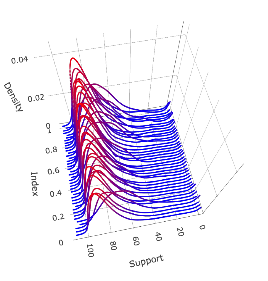
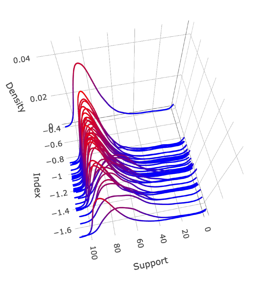
Figure B.8: Data visualization for age-at-death densities for $40$ countries at the calendar year 2010. The left panel shows the observed densities at random order while the right panel plots the observed densities against the estimated index values from the proposed Index Fréchet Regression (IFR) model.

The plots of the observed and estimated age-at-death densities over the support of age $[0,110]$ and against the estimated index values, aka the first estimated sufficient predictor, are shown in Figure B.9. It is interesting to observe that the estimated index values are associated with the location and variation features of the age-at-death distributions. Specifically, with the increase in the values of the index, the mean of the mortality distribution increases non-linearly while the standard deviation diminishes, indicating the death age more concentrates between 70 and 80. This finding is in line with the observations of Zhang et al., (2021), who employed several sufficient dimension reduction (SDR) techniques to the mortality distributions.

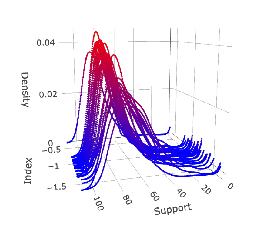
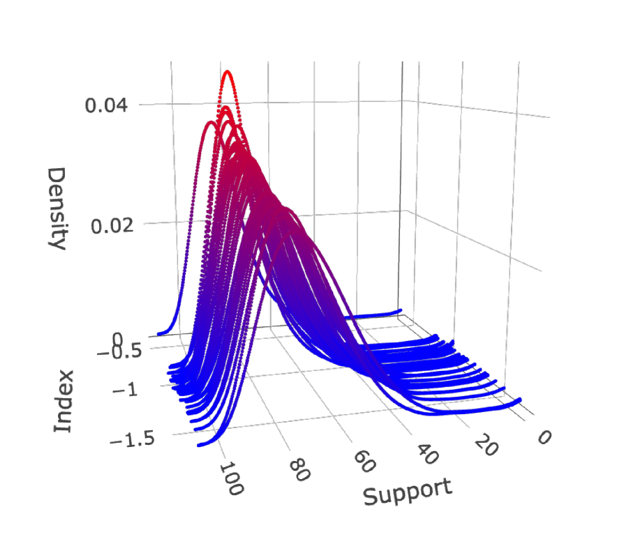
Figure B.9: The observed and estimated age-at-death distributions for $40$ countries at the calendar year 2010 are displayed in the left and right panel of figure, respectively. The distributions are plotted over the support of the age interval $[0,110]$ against the index values estimated by the IFR model.

Further, the importance of various predictors can be inferred from the estimated coefficients $\bm{\widehat{\widebar{\theta}}}.$ As before we keep the first predictor ($X_{1}=$ Population density) with the corresponding coefficient $\hat{\theta}_{1}=0.0173>0$ in the model and test for the following hypothesis: $H_{0}:\theta_{02}=\dots=\theta_{0p}=0$ vs. $H_{1}$, the complement of $H_{0}$, which is the test for overall regression effect for object responses. Writing $\hat{\bm{\theta}}=(\hat{\theta}_{2},\dots,\hat{\theta}_{6}),$ the test statistic is constructed as $\tilde{T}_{n}=\hat{\bm{\theta}}^{\top}(\widehat{\Lambda}^{\ast}_{B})^{-1}\hat{\bm{\theta}}\overset{approx.}{\sim}\chi^{2}_{5}$ under $H_{0}$ (see Section 5.1), where $\widehat{\Lambda}^{\ast}_{B}$ is the bootstrap estimator for asymptotic covariance matrix as described in Proposition 5. The null hypothesis is rejected at level $\alpha$ if $\tilde{T}_{n}>\chi^{2}_{5}(1-\alpha).$ From our analysis, $\tilde{T}_{n}=18.883>11.0705=\chi^{2}_{5}(1-\alpha)$ for the level $\alpha=0.05.$ The p-value is actually $0.002$ and the null hypothesis is thus clearly rejected, demonstrating there is a regression effect. Upon further analysis it is found that the most significant predictors, in order, are $X_{2}=$ Fertility rate, total (births per woman), $X_{3}=$ GDP per capita, at Purchasing Power Parity (PPP), and $X_{5}=$ Current health expenditure (% of GDP).

We proceed to compare fits for the year 2010 from the IFR model with the Global Fréchet Regression (GFR) model with the $6-$dimensional predictors, as well as with three separate Local Fréchet Regression (LFR) models, where the three important predictors Fertility Rate, GDP per capita and Health Expenditure are considered in each LFR model separably as univariate predictors. The global Fréchet model suffers from model-induced bias, while the local linear Fréchet Regression models with individual univariate predictors lack relevant information from other variables. The IFR model is a semiparametric approach that combines the strengths of both of these models. Figure B.10 displays the observed as well as the fitted distributions (as densities) for these five models. The superiority of the IFR model compared to the local linear Fréchet fits, using only the relatively important predictor variables individually indicates that all predictors simultaneously play an important role in the overall prediction through the estimated index $\textbf{x}^{\top}\bm{\widehat{\widebar{\theta}}}.$

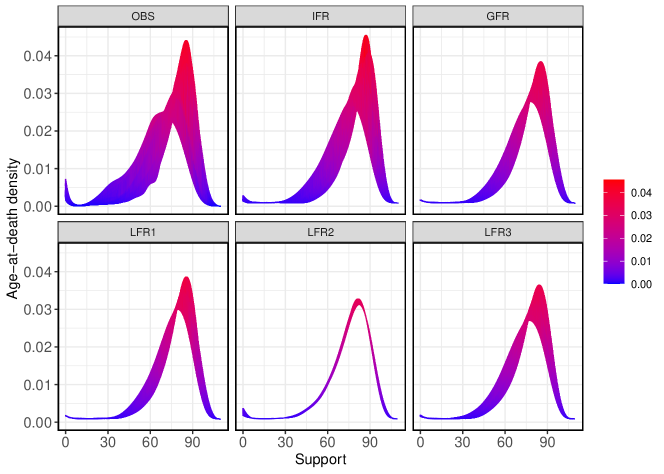
Figure B.10: Figure displaying the observed and predicted smooth densities. Clockwise, from top-left the observed densities (OBS), the fitted densities using Index Frechet Regression (IFR), Global Fréchet Regression (GFR), and Local Fréchet Regression (LFR). The predictors used for the LFR fits are Fertility Rate (LFR1), GDP per capita (LFR2) and Health Expenditures (LFR3), respectively. Densities are color-coded (blue to red indicating low to high) by the mode of the age-at-death distribution.

To study the effect of the most important predictors, GDP per capita, fertility rate, and Health expenditure percentage on the age-of-death densities, we fitted the IFR model when varying the value of one predictor, while keeping the other two fixed at their mean levels.

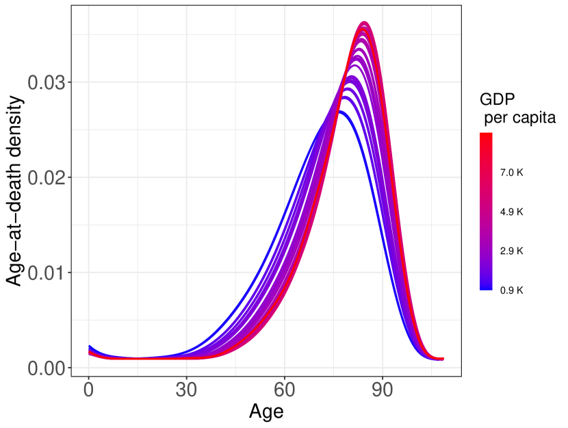
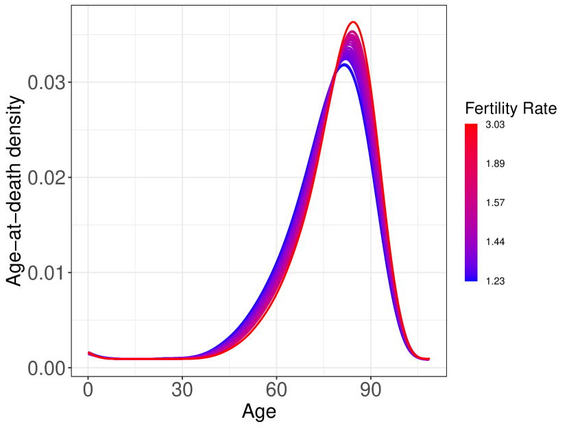
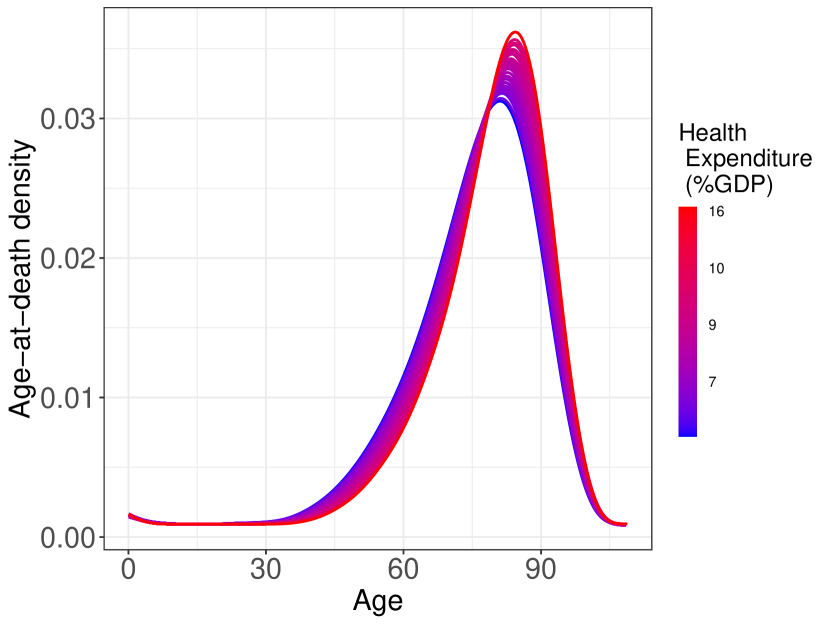
Figure B.11: Figure showing the effects of the significant predictors $X_{3}=$ GDP per capita, $X_{2}=$ Fertility rate, and $X_{5}=$ Current health expenditure. The left panel shows the change in density with changing value of $X_{3}$ from low (blue) to high (red), when $X_{2}$ and $X_{5}$ are fixed at their mean level, and analogously for middle and right panels.

For example, the left-most panel of Figure B.11 illustrates how the age-at-death density changes with increasing levels of GDP per capita, while the other two predictors are kept fixed. The fitted densities are color coded such that blue to red indicates a smaller to a larger value of GDP. We find that smaller values of GDP are associated with left-shifted age-at-death distributions for the population. For increasing levels of health expenditure per capita and fertility rates, the age-at-death densities also shift rightwards, but to a lesser extent.

Finally, to illustrate the out-of-sample prediction performance of the proposed IFR model, we randomly split the dataset into a training set with sample size $n_{\text{train}}=20$ and a test set with the remaining $n_{\text{test}}=20$ subjects. The IFR method was implemented as follows: For any given unit direction $\bm{\bar{\theta}}\in\bar{\Theta},$ we partition the domain of the projections into $M$ equal-width non-overlapping bins and consider the representative observations $\tilde{\textbf{X}}_{l}$ and $\tilde{Y}_{l}$ for the data points belonging to the $l-$th bin. The “true” index parameter is estimated as $\bm{\widehat{\widebar{\theta}}}$ as per equation (2.11). We then take the fitted objects obtained from the training set and predict the responses in the test set using the covariates present in the test set. As a measure of the efficacy of the fitted model, we compute the root mean squared prediction error (RMPE) as

RMPE $$=\left[\frac{1}{M_{n_{\text{test}}}}\sum_{i=1}^{M_{n_{\text{test}}}}d_{W}^{2}\left(\tilde{Y}_{l}^{\text{test}},\hat{m}_{\oplus}(\tilde{\mathbf{X}}_{l}^{\text{test}\intercal}\bm{\widehat{\widebar{\theta}}},\bm{\widehat{\widebar{\theta}}})\right)\right]^{1/2},$$ (B.50)

where $\tilde{Y}_{l}^{\text{test}}$ and $\hat{m}_{\oplus}(\tilde{\mathbf{X}}_{l}^{\text{test}\intercal}\bm{\widehat{\widebar{\theta}}},\bm{\widehat{\widebar{\theta}}})$ denote, respectively, the $l^{\text{th}}$ observed and predicted responses in the test set, evaluated at the binned observation $\tilde{\mathbf{X}}_{l}^{\text{test}}.$ For any two distribution objects $F,G\in(\Omega,d_{W})$, the Wasserstein-2 distance is given by

$$d_{W}(F,G)=\int_{0}^{1}(F^{-1}(s)-G^{-1}(s))^{2}ds,$$

where $F^{-1}$ and $G^{-1}$ are the quantile functions corresponding to $F$ and $G$ respectively. We repeat this process $500$ times, and compute RMPE for each split for the subjects separately. The mean and sd of the RMPE over the repetitions are shown in Table 7 for the IFR method, as well as for the GFR and individual LFR fits.

Table 7: Mean and sd (in parenthesis) of the RMPE as given in (B.50) comparing the performance of various Fréchet regression models: Index Frćhet Regression (IFR), Global Fréchet Regression (GFR), Local Fréchet Regression (LFR). The predictors used for the three individual LFR fits are Fertility Rate, GDP per capita at PPP, and Health Expenditure, respectively, as indicated in parentheses.

IFR	GFR	LFR1 (on Fertility Rate)	LFR2 (on GDP per Capita-PPP)	LFR3 (on Health Expenditure)
0.178 (0.0552)	0.287 (0.0671)	0.491 (0.0605)	0.603 (0.0654)	0.339 (0.0565)

Using out-of-sample performance, the IFR model emerges as the best model, as the average RMPE of $0.178$ is much lower than that of any of the other models.

S.3.2. Emotional well-being for unemployed workers: Compositional data as random object responses

We demonstrate the proposed IFR method for the analysis of mood compositional data. Compositional data are random vectors with non-negative components, where the components of these vectors sum to 1. With a square-root transformation of the components, compositional vectors can be transformed to unit vectors that lie on the positive segment of a sphere $S^{p-1}$ if the compositional vectors are $p-$dimensional (Scealy and Welsh,, 2011, 2014). Thus one can represent compositional data as manifold-valued objects that lie on the surface of a sphere. The data used for this application were collected in the Survey of Unemployed Workers in New Jersey (Krueger et al.,, 2011) conducted in the fall of 2009 and the beginning of 2010, during which the unemployment rate in the US peaked at 10% after the financial crisis of 2007 – 2008; similar data were used to illustrate longitudinal compositional methods in Dai et al., (2021). We note that here the object-valued responses lie on a manifold (sphere) with positive curvature. Thus the sufficient (but not necessary) condition for assumption (A5) that the underlying metric space behaves like a CAT(0) space is not satisfied. This example thus provides a check on the behavior of IFR when the random objects are situated in a positively curved space.

Unemployed workers belonging to a stratified random sample were surveyed at entry into the study, where we analyzed the data for $n=3301$ workers with complete measurements. A key variable in the survey was the proportion of time the workers spent in each of the four moods: bad, low/irritable, mildly pleasant, and very good while at home; we use this 4-dimensional compositional vector as the response. Formally, the composition measurement of interest is $Z=(Z_{1},Z_{2},Z_{3},Z_{4})^{\intercal}$, where $Z_{j}$ is the proportion of time a worker spent in the $j$-th mood when at home, $j=1,\dots,4.$ The square-root transformed compositional data

$$Y=(Y_{1},Y_{2},Y_{3},Y_{4})^{\intercal}=(\sqrt{Z}_{1},\sqrt{Z}_{2},\sqrt{Z}_{3},\sqrt{Z}_{4})^{\top},$$

lie on the sphere $\mathcal{S}^{3}$. We adopt the geodesic metric on this sphere $d_{g}(y,y^{\ast})=\arccos(y^{\top}y^{\ast}).$

These square root transformed compositional data are treated as the object responses in a regression model with the following 10 baseline predictors obtained from the questionnaire, reflecting various socio-economic and demographic information: (1) life satisfaction (discrete with levels 0-3, 3 meaning most satisfied) (2) highest education level (discrete with levels 0-5, indicating high school or less, high school diploma or equivalent, college education, college diploma, graduate school, and graduate degree, respectively), (3) marital status (discrete with levels 0-5, indicating single (never married), married, separated, divorced, widowed, and domestic partnership (living together but not married), respectively), (4) number of children (discrete), (5) the number of people in the household (discrete), (6) total annual household income (continuous), (7) hours per week working at the last job (continuous), (8) how the last job ended (discrete with levels 0-2 lost job, quit job, and temporary job ended, respectively), (9) weeks spent looking for work (continuous), and (10) credit card balance (continuous).

For these data, the IFR model produces the coefficient estimates

$$\bm{\widehat{\widebar{\theta}}}=(0.483,0.134,-0.166,-0.190,0.042,0.303,0.075,0.230,0.662,-0.307)^{\intercal}.$$

The estimated coefficients can be used to obtain interpretable visualizations of the effect of the individual predictors on the compositional response through the (estimated) single index link function, which can further lead to effective inference for the proposed IFR model. For example, we illustrate below (Figure B.12) the effect of the predictor “life satisfaction” on the mood compositional data. To this end, the IFR model is fitted over varying levels of life satisfaction, from low (0) to high (3), while the other predictors are fixed at their median levels. We observe an association between a lower life satisfaction level with a higher proportion of bad mood, while a higher value of life satisfaction is associated with a better mood when all of the other predictors are fixed.

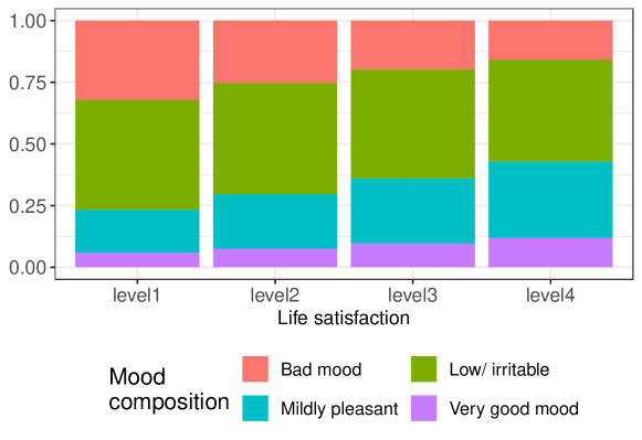
Figure B.12: A stacked barplot showing the effect of life satisfaction, from Level 1 (0) to Level 4 (3), on the mood composition, when all the other predictor levels are kept fixed. A higher life satisfaction level is associated with a larger proportion of good mood.

The predictive performance of the model is computed based on the root mean prediction error (RMPE) as

$$\text{RMPE}=\left[\frac{1}{M_{n_{\text{test}}}}\sum_{i=1}^{M_{n_{\text{test}}}}d_{g}^{2}\left(\tilde{Y}_{l}^{\text{test}},\hat{m}_{\oplus}(\tilde{\textbf{X}}_{l}^{\top}\bm{\widehat{\widebar{\theta}}},\bm{\widehat{\widebar{\theta}}})\right)\right]^{1/2},$$

where $\tilde{Y}_{l}^{\text{test}}$ and $\hat{m}_{\oplus}(\tilde{\textbf{X}}_{l}^{\top}\bm{\widehat{\widebar{\theta}}})$ denote, respectively, the $l^{\text{th}}$ observed and predicted responses in the test set, evaluated at the binned average $\tilde{\textbf{X}}_{l}.$ We repeat this process $200$ times, and compute RMPE for each split for the subjects separately. For comparison purposes, we fit the data with the other applicable object regression methods, namely, the global Fréchet regression (GFR) method with the four-dimensional mood-compositional data as the response residing on the surface of the sphere $S^{3}\subset\mathbb{R}^{4}$, coupled with the 10-dimensional predictors; and individual local linear Fréchet regression (LFR) methods accommodating the afore-mentioned object response, while incorporating the continuous predictors total annual household income, hours per week working at the last job, weeks spent looking for work and credit card balance as univariate predictors. Like nonparametric regression, the LFR method does not work for discrete/ categorical predictors. We denote the results from the four individual univariate local regression by $\text{LFR}_{j}$, $j=1,2,3,4$, respectively. Table 8 summarizes the results.

Table 8: Mean and sd (in parenthesis) of root mean prediction error (RMPE) over $200$ repetitions, as obtained from the local fits of the index Fréchet regression (IFR) model, the global Fréchet regression (GFR) model, and four individual local linear Fréchet regression (LFR) models incorporating univariate continuous predictors. Here, $n_{\text{train}}$ and $n_{\text{test}}$ denote the sample sizes for the split training and testing datasets respectively.

$n_{\text{train}}$	$n_{\text{test}}$	IFR	GFR	$\text{LFR}_{1}$	$\text{LFR}_{2}$	$\text{LFR}_{3}$	$\text{LFR}_{4}$
$2201$	$1100$	$0.4779$ $(0.0720)$	$0.7661$ $(0.0418)$	$0.6771$ $(0.0021)$	$0.7220$ $(0.0450)$	$1.1127$ $(0.0910)$	$1.0122$ $(0.0810)$

We observe that the out-of-sample prediction error is quite low. In fact, it is very close to the average fitting error $(0.351)$, calculated as the average distance between the observed training sample and the predicted objects based on the covariates in the training sets, which supports the validity of the proposed IFR models.

Since in this example the object-valued responses lie on a manifold (sphere) with positive curvature, the sufficient (but not necessary) condition for assumption (A5) that the underlying metric space behaves like a CAT(0) space is not satisfied. However, the numerical performance of the IFR method is quite good, suggesting a certain degree of model robustness of the IFR method.

S.3.3. Additional results for the analysis of ADNI neuroimaging data

The individual effect of the significant predictors- stages of the disease, age, and total score, is illustrated. To this end, the IFR model is fitted over varying values of one predictor, while keeping the other two fixed at their mean levels.

For any $r\times r$ correlation matrix $Y$, the Fiedler value is the second smallest eigenvalue of the corresponding graph Laplacian matrix

$$L(Y)=D(Y)-A(Y).$$

Here $A(Y)=(Y-I_{r})_{+}$ is the adjacency matrix obtained by applying a threshold and setting the diagonal elements to zero, and $D(Y)={\rm diag}{A(Y)\mathbf{1}_{r}}$ is the degree matrix, where $I_{r}={\rm diag}{\mathbf{1}_{r}}$, $\mathbf{1}_{r}=(1,\dots,1)\intercal\in\mathbb{R}^{r}$, and $H_{+}=(\max\{H_{kl},0\})_{k,l=1\dots,r}$ for any matrix $H\in\mathbb{R}^{r\times r}.$ The Fiedler value corresponding to $Y$ is then given by the map $\lambda_{r-1}(L(Y))$, which produces the $(r-1)$th largest, i.e., second smallest eigen value of $L(Y)$. After fitting the proposed IFR model, the Fiedler values are calculated over varying values of age and total score. The left panel of Figure B.13 shows how the Fiedler value changes with increasing age, while the total score is kept fixed at its mean level, while the right panel shows the Fiedler values over the varying total scores for the fixed mean level of age.

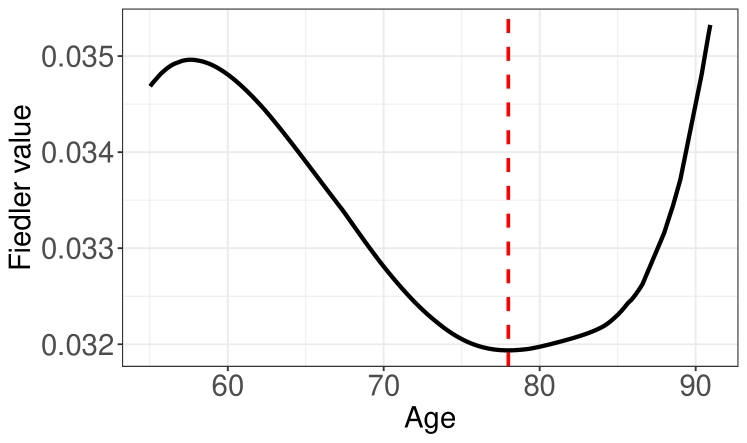
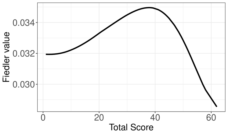
Figure B.13: Fiedler values as a function of age and total score, corresponding to the index Fréchet regression (IFR) fits for the correlation matrix-valued object responses. The left panel shows the change in the estimated Fiedler value for varying values of age ($X_{2}$) from low to high when $X_{4}$ (total score) is fixed at its mean level, with the minimum attained at 78 years of age marked by a red dashed line. The right panel shows the change in the total score for a fixed mean level of age.

In the age-varying Fielder value figure, a convex pattern can be seen around the minimum, which is attained at 78 years of age. This agrees with most studies that have found that functional connectivity decreases during normal aging processes before 80 years of age. Further, we observe that the decrease is reversed for older ages above $80.$ On the other hand, for a higher value of the total score, the Fielder values show a steep decreasing pattern.

Further, continuing from Section 5.1 in the main manuscript, we illustrate the $95\%$ confidence region for the coefficients $(\theta_{1},\theta_{2},\theta_{4})$ of the predictors: stages of the disease, age, and total score in a 3-dimensional plot in Figure B.14.

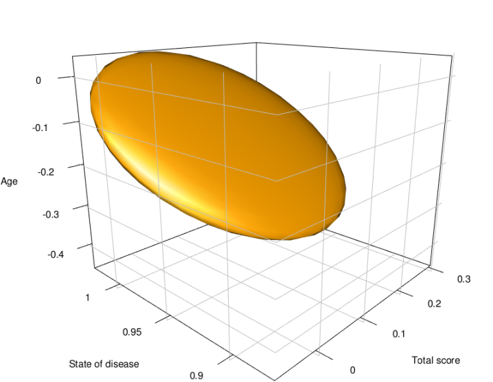
Figure B.14: The figure shows the 3-dimensional plot for the $95\%$ confidence region of $(\theta_{1},\theta_{2},\theta_{4})$: the coefficients of the effects of the predictors- age, total score, and stage of the disease, respectively.

S.3.4. Additional simulations for Euclidean responses

Here the object response of interest is assumed to lie in the Euclidean space. For generating the predictor vectors we consider a $5-$dimensional vector distributed as truncated multivariate normal distributions, where each of the components is truncated to lie between $[-10,10].$ The components are assumed to be correlated such that $X_{1}$ correlates with $X_{2}$ and $X_{3}$ with $r=0.5$, and $X_{2}$ and $X_{3}$ correlate with $r=0.25.$ The variances for each of the five components are $0.1.$ The empirical power against the sequence of alternatives in equation (3.10) increases steeply (see Figure B.15) as we deviate from the null hypothesis in equation (3.9) in Section 3 of the main manuscript, especially corresponding to higher sample size and under identity link.

The empirical power function, as we deviate from the null hypothesis in equation (3.9) is computed and illustrated in the left panel in Figure B.15. Empirical evidence suggests that the proposed test is consistent for a higher sample size of $n=1000$, and leads to the correct nominal level of the test.

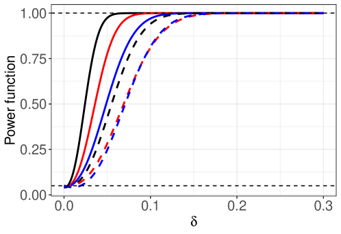
Figure B.15: Simulation for Euclidean response using different link functions showing the empirical power function for Euclidean responses. The black, red, and blue curves correspond to the identity, square, and exponential link functions used in the data-generating mechanism, respectively, while the dashed and solid patterns correspond to the varying sample sizes $n=100$ and $n=1000$, respectively. The level of the tests is $\alpha=0.05$ and is indicated by the dashed line parallel to the x-axis.

The consistency of the estimates is illustrated in Table 9 based on $500$ replications of the simulation scenario.

Table 9: Table showing bias and variance of $\bm{\widehat{\widebar{\theta}}}$ (measured in radians) based on $500$ replications for a Euclidean vector response. The predictors $X_{1},\dots,X_{5}$ are generated from a truncated multivariate normal distribution.

	link1 ($x\mapsto x$)		link2 ($x\mapsto x^{2}$)		link3 ($x\mapsto e^{x}$)
	bias	dev	bias	dev	bias	dev
$n=100$	0.013	0.061	0.025	0.048	0.037	0.029
$n=1000$	0.006	0.021	0.014	0.019	0.013	0.009

Further, the performance of the proposed method is compared to the classical Euclidean single index model fits. To this end, the R package np was called from Julia, for fitting the classical single index regression to the simulated Euclidean responses. The prediction performance of the classical single index fits, denoted by NP, is compared with that of the IFR method, as well as with a Global Fréchet Regression (GFR) method and four separate Local Frécet Regression (LFR) fits. The GFR method utilizes the multi-variate predictors while the four LFR methods treat each of the four-dimensional predictor components as a univariate predictor individually. Note that in all of the methods- NP, GFR, LFR - binning is not required. The mean and sd of the root mean prediction error (RMPE) over $200$ Monte Carlo simulation runs are reported in Table 10.

Table 10: Table showing the mean (sd in parenthesis) RMPE for various regression methods for simulated Euclidean responses. The methods compared are index Fréchet regression (IFR), classical Euclidean single index regression using the R package “np” (NP), global Fréchet Regression (GFR) with the 4-dimensional predictor, and four individual local linear Fréchet regression (LFR) models that treat each predictor components as a univariate predictor. The sample size is fixed at $n=1000$ and the RMPE are computed over $200$ Monte Carlo simulation runs.

	Identity link	Square link	Exponential link
IFR	0.0255 (0.0110)	0.1383 (0.1031)	0.1972 (0.1205)
NP	0.0187 (0.0201)	0.1117 (0.1077)	0.1578 (0.0442)
GFR	0.0003 (0.0018)	0.1465 (0.0299)	0.2181 (0.0748)
LFR1	0.0788 (0.0208)	0.2686 (0.0558)	0.3342 (0.1882)
LFR2	0.0784 (0.0204)	0.2627 (0.0540)	0.3237 (0.1912)
LFR3	0.0617 (0.0209)	0.2774 (0.0555)	0.3162 (0.1892)
LFR4	0.0730 (0.0197)	0.2694 (0.0561)	0.3664 (0.1888)

The data is simulated using three different generating mechanisms - the identity, squared, and exponential link functions, and the sample size $n=1000$ is considered. For the identity link function, i.e., when the simulated data is generated according to a linear model, the GFR method gives the lowest prediction error. This is indeed expected since the GFR boils down to a linear regression model when the object data are Euclidean. For other situations the NP method for the classical single index model outperforms the other methods, however, the proposed IFR method proves competitive with a comparable magnitude of the prediction error. The boxplot of the RMPEs for the above situations is shown in Figure B.16.

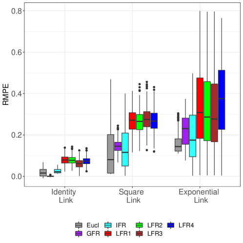
Figure B.16: Figure showing boxplot of RMPEs for various regression methods for simulated Euclidean responses. The methods compared are index Fréchet regression (IFR), classical Euclidean single index regression using the R package “np” (NP), global Fréchet Regression (GFR) with the 4-dimensional predictor, and four individual local linear Fréchet regression (LFR) models that treat each predictor components as a univariate predictor. The sample size is fixed at $n=1000$ and the RMPE are computed over $200$ Monte Carlo simulation runs.

S.3.5. Simulation results for adjacency matrix as random object responses

Here we consider responses that are adjacency matrices obtained for weighted networks and equipped with the Frobenius norm. We generated samples of networks with $m=10$ nodes, as one might encounter in brain networks, represented as weighted adjacency matrices. The predictors were sampled from a $4-$dimensional zero mean multivariate normal distribution with covariance matrix defined by ${\rm cor}(X_{1},X_{2})={\rm cor}(X_{1},X_{3})={\rm cor}(X_{2},X_{3})=0.3,$ and ${\rm cor}(X_{1},X_{4})={\rm cor}(X_{2},X_{4})=-0.4.$ and variances of all components equal to $0.25.$ Subsequently each of the components was truncated to lie between $[-5,5]$. The elements of the weighted adjacency matrices $Y=(Y_{qr})$ were then obtained as

$$Y_{qr}=\zeta(\textbf{x}^{\top}{\bm{\bar{\theta}_{0}}})+\epsilon_{qr},\ q,r=1,\dots,m,$$

where $\epsilon_{qr}$ are independently sampled errors and the link function $\zeta(\cdot)$ was taken as the expit function, i.e., $\zeta(\textbf{x}^{\top}{\bm{\bar{\theta}_{0}}})=1/(1+\exp(-\textbf{x}^{\top}{\bm{\bar{\theta}_{0}}})).$ For a given index $\textbf{x}^{\top}{\bm{\bar{\theta}_{0}}},$ $\epsilon_{qr}$ was sampled from a uniform distribution on $[\max\{0,-\zeta(\textbf{x}^{\top}{\bm{\bar{\theta}_{0}}})\},\min\{1,1-\zeta(\textbf{x}^{\top}{\bm{\bar{\theta}_{0}}})\}]$. The matrix responses of interest were thus generated as $Y=\zeta(\textbf{x}^{\top}{\bm{\bar{\theta}_{0}}})I_{m}+\bm{\varepsilon},$ where $\bm{\varepsilon}=\left(\left(\epsilon_{qr}\right)\right)_{q,r=1,\dots,m}$ as generated above and $I_{m}$ is the $m\times m$ identity matrix.

Table 11: Table showing bias and deviance of $\hat{\theta}$ (measured in radians, as per eqrefsimul:bias:var) based on $500$ replications for weighted adjacency matrix responses.

	link $(x\mapsto 1/(1+\exp(-x))$
	bias	dev	avg. MSD
$n=100$	0.044	0.052	0.672
$n=1000$	0.021	0.019	0.041

Table 11 presents the bias and variance of the estimator computed based on $500$ replication of the data generating process. The mean squared deviation (MSD) was computed as the average distance between the true and estimated adjacency matrices, similar to (27). The average mean squared deviation (MSD) over $500$ simulation runs is quite low. With a higher sample size, the estimates seem to perform better consistently. We also note here that the non-zero correlation among the components of the predictor vector does not influence the performance of the nonparametric regression fit negatively.

Figure B.17 shows the empirical power function as we deviate from the null hypothesis in  (22) for two different sample sizes. Empirical evidence suggests that the proposed test is consistent for a higher sample size of $n=1000$, and leads to the correct empirical level of the test.

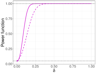
Figure B.17: Simulation for adjacency matrix response for different sample sizes. The figure displays the empirical power as function of $\delta$ for weighted adjacency matrix responses based on sample sizes $n=100$ and $n=1000,$ in dashed and solid lines, respectively. The magenta color corresponds to the expit link function used to generate the data, while the dashed and solid pattern correspond to the varying sample sizes $n=100$ and $n=1000$, respectively. The level of the tests is $\alpha=0.05$ and is indicated by the dashed line parallel to the x-axis.

References

- Afsari, (2011) Afsari, B. (2011). Riemannian center of mass: existence, uniqueness, and convexity. Proceedings of the American Mathematical Society, 139(2):655–673.
- Allen et al., (2014) Allen, E., Damaraju, E., Plis, S., Erhardt, E., Eichele, T., and Calhoun, V. (2014). Tracking whole-brain connectivity dynamics in the resting state. Cerebral Cortex, 24(3):663–676.
- Andrews-Hanna et al., (2010) Andrews-Hanna, J. R., Reidler, J. S., Sepulcre, J., Poulin, R., and Buckner, R. L. (2010). Functional-anatomic fractionation of the brain’s default network. Neuron, 65(4):550–562.
- Bhattacharjee and Müller, (2022) Bhattacharjee, S. and Müller, H.-G. (2022). Concurrent object regression. Electronic Journal of Statistics, 16(2):4031–4089.
- Bhattacharjee and Müller, (2022) Bhattacharjee, S. and Müller, H.-G. (2022). Supplement to “single index fréchet regression”.
- Bhattacharya and Patrangenaru, (2003) Bhattacharya, R. and Patrangenaru, V. (2003). Large sample theory of intrinsic and extrinsic sample means on manifolds. Annals of Statistics, 31(1).
- Bhattacharya and Patrangenaru, (2005) Bhattacharya, R. and Patrangenaru, V. (2005). Large sample theory of intrinsic and extrinsic sample means on manifolds:II. The Annals of Statistics, 33(3):1225–1259.
- Buchinsky, (1995) Buchinsky, M. (1995). Estimating the asymptotic covariance matrix for quantile regression models a Monte Carlo study. Journal of Econometrics, 68(2):303–338.
- Burago et al., (2001) Burago, D., Burago, I. D., Burago, Y., Ivanov, S., Ivanov, S. V., and Ivanov, S. A. (2001). A Course in Metric Geometry, volume 33. American Mathematical Society.
- Carroll et al., (1997) Carroll, R. J., Fan, J., Gijbels, I., and Wand, M. P. (1997). Generalized partially linear single-index models. Journal of the American Statistical Association, 92(438):477–489.
- Chang et al., (2010) Chang, Z., Xue, L., and Zhu, L. (2010). On an asymptotically more efficient estimation of the single-index model. Journal of Multivariate Analysis, 101(8):1898–1901.
- Chen et al., (2011) Chen, D., Hall, P., and Müller, H.-G. (2011). Single and multiple index functional regression models with nonparametric link. The Annals of Statistics, 39(3):1720–1747.
- Chen et al., (2020) Chen, Y., Gajardo, A., Fan, J., Zhong, Q., Dubey, P., Han, K., Bhattacharjee, S., and Müller, H.-G. (2020). frechet: Statistical Analysis for Random Objects and Non-Euclidean Data. R package version 0.2.0.
- Chen and Müller, (2022) Chen, Y. and Müller, H.-G. (2022). Uniform convergence of local fréchet regression with applications to locating extrema and time warping for metric space valued trajectories. The Annals of Statistics, 50(3):1573–1592.
- Cook, (1994) Cook, R. D. (1994). Using dimension-reduction subspaces to identify important inputs in models of physical systems. In Proceedings of the Section on Physical and Engineering Sciences, pages 18–25.
- Cui et al., (2011) Cui, X., Härdle, W. K., and Zhu, L. (2011). The EFM approach for single-index models. The Annals of Statistics, 39(3):1658–1688.
- Dai et al., (2021) Dai, X., Lin, Z., and Müller, H.-G. (2021). Modeling sparse longitudinal data on riemannian manifolds. Biometrics, 77(4):1328–1341.
- Damoiseaux et al., (2012) Damoiseaux, J. S., Prater, K. E., Miller, B. L., and Greicius, M. D. (2012). Functional connectivity tracks clinical deterioration in Alzheimer’s disease. Neurobiology of Aging, 33(4):828–e19.
- Davison and Hinkley, (1997) Davison, A. C. and Hinkley, D. V. (1997). Bootstrap Methods and their Applications. Cambridge University Press.
- Delicado and Vieu, (2017) Delicado, P. and Vieu, P. (2017). Choosing the most relevant level sets for depicting a sample of densities. Computational Statistics, 32(3):1083–1113.
- Fan and Gijbels, (1996) Fan, J. and Gijbels, I. (1996). Local Polynomial Modelling and Its Applications. Chapman & Hall/CRC.
- Fan and Huang, (2005) Fan, J. and Huang, T. (2005). Profile likelihood inferences on semiparametric varying-coefficient partially linear models. Bernoulli, 11(6):1031–1057.
- Ferraty et al., (2011) Ferraty, F., Park, J., and Vieu, P. (2011). Estimation of a functional single index model. In Recent Advances in Functional Data Analysis and Related Topics, pages 111–116. Springer.
- Ferreira and Busatto, (2013) Ferreira, L. R. K. and Busatto, G. F. (2013). Resting-state functional connectivity in normal brain aging. Neuroscience & Biobehavioral Reviews, 37(3):384–400.
- Fréchet, (1948) Fréchet, M. R. (1948). Les éléments aléatoires de nature quelconque dans un espace distancié. Annales de l’institut Henri Poincaré, 10(4):215–310.
- Friedman and Stuetzle, (1981) Friedman, J. H. and Stuetzle, W. (1981). Projection pursuit regression. Journal of the American Statistical Association, 76(376):817–823.
- Gao and Liang, (1997) Gao, J. and Liang, H. (1997). Statistical inference in single-index and partially nonlinear models. Annals of the Institute of Statistical Mathematics, 49(3):493–517.
- Ghosal et al., (2021) Ghosal, A., Meiring, W., and Petersen, A. (2021). Fréchet single index models for object response regression. arXiv preprint arXiv:2108.06058.
- Gonçalves and White, (2005) Gonçalves, S. and White, H. (2005). Bootstrap standard error estimates for linear regression. Journal of the American Statistical Association, 100(471):970–979.
- Hall, (1989) Hall, P. (1989). On projection pursuit regression. The Annals of Statistics, 17(2):573–588.
- Härdle et al., (1993) Härdle, W., Hall, P., and Ichimura, H. (1993). Optimal smoothing in single-index models. The Annals of Statistics, 28(1):157–178.
- Härdle and Stoker, (1989) Härdle, W. and Stoker, T. M. (1989). Investigating smooth multiple regression by the method of average derivatives. Journal of the American Statistical Association, 84(408):986–995.
- Hristache et al., (2001) Hristache, M., Juditsky, A., and Spokoiny, V. (2001). Direct estimation of the index coefficient in a single-index model. The Annals of Statistics, 29(3):595–623.
- Huh and Park, (2002) Huh, J. and Park, B. (2002). Likelihood-based local polynomial fitting for single-index models. Journal of Multivariate Analysis, 80(2):302–321.
- Ichimura, (1993) Ichimura, H. (1993). Semiparametric least squares (SLS) and weighted SLS estimation of single-index models. Journal of Econometrics, 58(1-2):71–120.
- Jiang and Wang, (2011) Jiang, C.-R. and Wang, J.-L. (2011). Functional single index models for longitudinal data. The Annals of Statistics, 39(1):362–388.
- Kato, (2011) Kato, K. (2011). A note on moment convergence of bootstrap M-estimators. Statistics & Decisions, 28(1):51–61.
- Kereta et al., (2020) Kereta, Ž., Klock, T., and Naumova, V. (2020). Nonlinear generalization of the monotone single index model. Information and Inference: A Journal of the IMA.
- Kloeckner, (2010) Kloeckner, B. (2010). A geometric study of Wasserstein spaces: Euclidean spaces. Annali della Scuola Normale Superiore di Pisa-Classe di Scienze, 9(2):297–323.
- Krueger et al., (2011) Krueger, A. B., Mueller, A., Davis, S. J., and Şahin, A. (2011). Job search, emotional well-being, and job finding in a period of mass unemployment: Evidence from high-frequency longitudinal data [with comments and discussion]. Brookings Papers on Economic Activity, pages 1–81.
- Kuchibhotla and Patra, (2020) Kuchibhotla, A. K. and Patra, R. K. (2020). Efficient estimation in single index models through smoothing splines. Bernoulli, 26(2):1587 – 1618.
- Kueper et al., (2018) Kueper, J. K., Speechley, M., and Montero-Odasso, M. (2018). The Alzheimer’s disease assessment scale–cognitive subscale (adas-cog): modifications and responsiveness in pre-dementia populations. a narrative review. Journal of Alzheimer’s Disease, 63(2):423–444.
- Li and Wang, (2007) Li, B. and Wang, S. (2007). On directional regression for dimension reduction. Journal of the American Statistical Association, 102(479):997–1008.
- Li, (1991) Li, K.-C. (1991). Sliced inverse regression for dimension reduction. Journal of the American Statistical Association, 86(414):316–327.
- Li and Duan, (1989) Li, K.-C. and Duan, N. (1989). Regression analysis under link violation. The Annals of Statistics, 17(1):1009–1052.
- Liang et al., (2010) Liang, H., Liu, X., Li, R., and Tsai, C.-L. (2010). Estimation and testing for partially linear single-index models. The Annals of Statistics, 38(6):3811.
- Lin and Kulasekera, (2007) Lin, W. and Kulasekera, K. (2007). Identifiability of single-index models and additive-index models. Biometrika, 94(2):496–501.
- Lin and Müller, (2019) Lin, Z. and Müller, H.-G. (2019). Total variation regularized fréchet regression for metric-space valued data. arXiv preprint arXiv:1904.09647.
- Lopez et al., (2013) Lopez, O., Patilea, V., and Van Keilegom, I. (2013). Single index regression models in the presence of censoring depending on the covariates. Bernoulli, 19(3):721–747.
- Marron and Alonso, (2014) Marron, J. S. and Alonso, A. M. (2014). Overview of object oriented data analysis. Biometrical Journal, 56(5):732–753.
- Müller, (2016) Müller, H.-G. (2016). Peter Hall, functional data analysis and random objects. The Annals of Statistics, 44(5):1867–1887.
- Nishiyama, (2010) Nishiyama, Y. (2010). Moment convergence of M-estimators. Statistica Neerlandica, 64(4):505–507.
- Novo et al., (2019) Novo, S., Aneiros, G., and Vieu, P. (2019). Automatic and location-adaptive estimation in functional single-index regression. Journal of Nonparametric Statistics, 31(2):364–392.
- Patrangenaru and Ellingson, (2015) Patrangenaru, V. and Ellingson, L. (2015). Nonparametric Statistics on Manifolds and their Applications to Object Data Analysis. CRC Press.
- Pennec, (2018) Pennec, X. (2018). Barycentric subspace analysis on manifolds. Annals of Statistics, 46(6A):2711–2746.
- Petersen et al., (2019) Petersen, A., Deoni, S., and Müller, H.-G. (2019). Fréchet estimation of time-varying covariance matrices from sparse data, with application to the regional co-evolution of myelination in the developing brain. The Annals of Applied Statistics, 13(1):393–419.
- Petersen et al., (2021) Petersen, A., Liu, X., and Divani, A. A. (2021). Wasserstein -tests and confidence bands for the fréchet regression of density response curves. The Annals of Statistics, 49(1):590–611.
- Petersen and Müller, (2019) Petersen, A. and Müller, H.-G. (2019). Fréchet regression for random objects with Euclidean predictors. The Annals of Statistics, 47(2):691–719.
- Peyré, (2009) Peyré, G. (2009). Manifold models for signals and images. Computer Vision and Image Understanding, 113(2):249–260.
- Scealy and Welsh, (2011) Scealy, J. and Welsh, A. (2011). Regression for compositional data by using distributions defined on the hypersphere. Journal of the Royal Statistical Society: Series B (Statistical Methodology), 73(3):351–375.
- Scealy and Welsh, (2014) Scealy, J. and Welsh, A. (2014). Colours and cocktails: Compositional data analysis. Australian & New Zealand Journal of Statistics, 56(2):145–169.
- Schötz, (2019) Schötz, C. (2019). Convergence rates for the generalized frćhet mean via the quadruple inequality. Electronic Journal of Statistics, 13(2):4280–4345.
- Schötz, (2020) Schötz, C. (2020). Regression in nonstandard spaces with fréchet and geodesic approaches. arXiv preprint arXiv:2012.13332.
- Shao and Tu, (2012) Shao, J. and Tu, D. (2012). The Jackknife and Bootstrap. Springer Science & Business Media.
- Silverman, (1978) Silverman, B. W. (1978). Weak and strong uniform consistency of the kernel estimate of a density and its derivatives. The Annals of Statistics, 6(1):177 – 184.
- Small, (2012) Small, C. G. (2012). The Statistical Theory of Shape. Springer Science & Business Media.
- Stoker, (1986) Stoker, T. M. (1986). Consistent estimation of scaled coefficients. Econometrica: Journal of the Econometric Society, 54(6):1461–1481.
- Sturm, (2003) Sturm, K.-T. (2003). Probability measures on metric spaces of nonpositive. Heat Kernels and Analysis on Manifolds, Graphs, and Metric Spaces: Lecture Notes from a Quarter Program on Heat Kernels, Random Walks, and Analysis on Manifolds and Graphs: April 16-July 13, 2002, Emile Borel Centre of the Henri Poincaré Institute, Paris, France, 338:357.
- Thomas Yeo et al., (2011) Thomas Yeo, B., Krienen, F. M., Sepulcre, J., Sabuncu, M. R., Lashkari, D., Hollinshead, M., Roffman, J. L., Smoller, J. W., Zöllei, L., and Polimeni, J. R. (2011). The organization of the human cerebral cortex estimated by intrinsic functional connectivity. Journal of Neurophysiology, 106(3):1125–1165.
- Tsochantaridis et al., (2004) Tsochantaridis, I., Hofmann, T., Joachims, T., and Altun, Y. (2004). Support vector machine learning for interdependent and structured output spaces. In Proceedings of the Twenty-first International Conference on Machine Learning, page 104.
- Van der Vaart and Wellner, (2000) Van der Vaart, A. and Wellner, J. (2000). Weak Convergence and Empirical Processes: with Applications to Statistics (Springer Series in Statistics). Springer.
- Wang et al., (2010) Wang, J.-L., Xue, L., Zhu, L., and Chong, Y. S. (2010). Estimation for a partial-linear single-index model. The Annals of Statistics, 38(1):246–274.
- Xia, (2007) Xia, Y. (2007). A constructive approach to the estimation of dimension reduction directions. The Annals of Statistics, 35(6):2654–2690.
- Xia and Härdle, (2006) Xia, Y. and Härdle, W. (2006). Semi-parametric estimation of partially linear single-index models. Journal of Multivariate Analysis, 97(5):1162–1184.
- Xia et al., (2009) Xia, Y., Tong, H., Li, W. K., and Zhu, L.-X. (2009). An adaptive estimation of dimension reduction space. In Exploration Of A Nonlinear World: An Appreciation of Howell Tong’s Contributions to Statistics, pages 299–346. World Scientific.
- Ying and Yu, (2020) Ying, C. and Yu, Z. (2020). Fréchet sufficient dimension reduction for random objects. arXiv preprint arXiv:2007.00292.
- Yu and Ruppert, (2002) Yu, Y. and Ruppert, D. (2002). Penalized spline estimation for partially linear single-index models. Journal of the American Statistical Association, 97(460):1042–1054.
- Zhang et al., (2010) Zhang, H.-Y., Wang, S.-J., Liu, B., Ma, Z.-L., Yang, M., Zhang, Z.-J., and Teng, G.-J. (2010). Resting brain connectivity: changes during the progress of Alzheimer disease. Radiology, 256(2):598–606.
- Zhang et al., (2021) Zhang, Q., Xue, L., and Li, B. (2021). Dimension reduction and data visualization for Fréchet regression. arXiv preprint arXiv:2110.00467.
- Zhao et al., (2017) Zhao, W., Lian, H., and Liang, H. (2017). Quantile regression for the single-index coefficient model. Bernoulli, 23(3):1997 – 2027.
- Zhao et al., (2020) Zhao, W., Zhang, F., Li, R., and Lian, H. (2020). Principal single-index varying-coefficient models for dimension reduction in quantile regression. Journal of Statistical Computation and Simulation, 90(5):800–818.
- Zhou and He, (2008) Zhou, J. and He, X. (2008). Dimension reduction based on constrained canonical correlation and variable filtering. The Annals of Statistics, 36(4):1649–1668.
- Zhu and Xue, (2006) Zhu, L. and Xue, L. (2006). Empirical likelihood confidence regions in a partially linear single-index model. Journal of the Royal Statistical Society: Series B (Statistical Methodology), 68(3):549–570.
- Zhu and Zhu, (2009) Zhu, L.-P. and Zhu, L.-X. (2009). On distribution-weighted partial least squares with diverging number of highly correlated predictors. Journal of the Royal Statistical Society: Series B (Statistical Methodology), 71(2):525–548.