Seismic wave propagation and inversion with Neural Operators

Abstract

Seismic wave propagation forms the basis for most aspects of seismological research, yet solving the wave equation is a major computational burden that inhibits the progress of research. This is exacerbated by the fact that new simulations must be performed when the velocity structure or source location is perturbed. Here, we explore a prototype framework for learning general solutions using a recently developed machine learning paradigm called Neural Operator. A trained Neural Operator can compute a solution in negligible time for any velocity structure or source location. We develop a scheme to train Neural Operators on an ensemble of simulations performed with random velocity models and source locations. As Neural Operators are grid-free, it is possible to evaluate solutions on higher resolution velocity models than trained on, providing additional computational efficiency. We illustrate the method with the 2D acoustic wave equation and demonstrate the method’s applicability to seismic tomography, using reverse mode automatic differentiation to compute gradients of the wavefield with respect to the velocity structure. The developed procedure is nearly an order of magnitude faster than using conventional numerical methods for full waveform inversion.

Keywords: wave propagation, forward model, inverse tomography, Fourier neural operator

1 Introduction

The simulation of seismic wave propagation through Earth’s interior underlies most aspects of seismological research, from the simulation of strong ground shaking due to large earthquakes (Rodgers et al., 2019; Graves and Pitarka, 2016), to imaging the subsurface velocity structure (Tape et al., 2009; Virieux and Operto, 2009; Fichtner et al., 2009; Lee et al., 2014; Gebraad et al., 2020), to derivation of earthquake source properties (Duputel et al., 2015; Ye et al., 2016; Wang and Zhan, 2020). The compute costs associated with these wavefield simulations are substantial, and for reasons of computational efficiency, 1D models are often used, even when better 3D velocity models are available. As a result, seismic wave simulations are often the limiting factor in the pace of geophysical research.

Recently, deep learning approaches have been explored with the goal of solving various geophysical partial differential equations (Smith et al., 2020; Moseley et al., 2020a, b, 2021). Beyond the goal of accelerating compute capabilities, such physics-informed neural networks may offer other advantages such as grid-independence, low memory overhead, differentiability, and on-demand solutions. These properties can then result in deep learning being used to solve geophysical inverse problems (Zhu et al., 2020; Zhang and Gao, 2021; Xiao et al., 2021; Smith et al., 2021), as a wider selection of algorithms and frameworks then are available for use, such as approximate Bayesian inference techniques like variational inference.

One of the major challenges associated with wave propagation is that a new simulation must be performed whenever the properties of the source or velocity structure are perturbed in some way. This alone substantially increases the necessary compute costs, making some problems prohibitively expensive even if they are mathematically or physically tractable. For the most part, these limitations have been accepted as an inevitable part of seismology, but now physics-informed machine learning approaches have started to offer some pathways for moving beyond this issue. For example, Smith et al. (2020) use a deep neural network to solve the Eikonal equation for any source-receiver pair by taking these locations as input. This then can be exploited for hypocenter inversion by allowing for gradients of the travel time field to be computed with respect to the source location (Smith et al., 2021). However, these models are relatively inefficient to train and even then, are only able to learn approximate solution operators to the differential equations.

The aforementioned limitations may seem surprising, but result from a basic attribute of neural networks that in fact makes them ill-suited for solving differential equations. Specifically, neural networks are designed for learning maps between two finite dimensional spaces, while learning a general solution operator for a differential equation requires the ability to map between two infinite dimensional spaces (i.e. function spaces). A paradigm for learning maps between function spaces was recently developed (Li et al., 2020b, a, 2021), and has been termed Neural Operator. The general idea behind these models is that they have shared parameters over all possible functions describing the initial conditions, which allows them operate on functions, even when the inputs are a numerically discretized representation of them.

Here, we explore the potential of Neural Operators in improving seismic wave propagation and inversion. We develop a prototype framework for training Neural Operators on the 2D acoustic wave equation and show that this approach provides a suite of tantalizing new advantages over conventional numerical methods for seismic wave propagation. This study provides a proof of concept of this technology and its application to seismology.

2 Preliminaries

For a given function $A$ and a Green’s function $G$, let $U$ denote the solution to a linear partial differential equation, i.e., the solution operator,

$$U(x)=(\mathcal{L}A)(x)=\int G(x,y)A(y)dy$$

where $\mathcal{L}$ is the corresponding linear operator. For example, suppose that the PDE to be solved is the acoustic wave equation; then $A$ could describe the velocity structure as well as the initial conditions. Neural operator generalizes this formulation to the nonlinear setting where a set of linear operators are sequentially applied to construct a general nonlinear solution operator. In its basic form, an $\ell$-layered neural operator is constructed as follows;

$$U(x)=\mathcal{L}_{\ell}\left(\sigma(\mathcal{L}_{\ell-1}\ldots\sigma\left(\mathcal{L}_{1}V\right)\ldots)\right)(x)$$

where $\mathcal{L}_{i}$ is such that for any function $V$, we have,

$$(\mathcal{L}_{i}V)(x)=W_{i}(x)+\int K_{i}(x,y)V(y)dy$$ (1)

Under this framework, $W_{i}(x)$ and $K_{i}(x,y)$ constitute the learnable components of the Neural Operator and allow for a solution to be produced for any prescribed function $A$. In a limited sense, Neural Operators can be viewed as generalized Green’s functions.

3 Methods

We designed a framework that applies Neural Operators to the 2D acoustic wave equation. The basic idea for this procedure is outlined schematically in Figure 1. A specific type of Neural Operator, called a Fourier Neural Operator (FNO; Li et al., 2021) receives a velocity model specified on an arbitrary, possibly irregular mesh, along with the coordinates of a point source. One of the main features of FNO is that the heavy calculations are performed in the frequency domain, which allows the convolutions in eq. 1 to be rapidly computed. The output of the FNO is the complete wavefield solution, which can be queried anywhere within the medium, regardless of whether the points lie on the input mesh.

The most basic component of the FNO is a Fourier block (Fig. 1), which first transforms an input function ($V$) to the Fourier domain. In the first layer of the network, $V$ is equal to the initial conditions, $A$. Then, a kernel ($K_{i}$) is computed specifically for this function and is truncated at low order, before performing the integration via multiplication. Finally, the result is transformed back and a non-linear activation function is applied, which concludes the Fourier block. For this study, the architecture of the FNO contains 4 sequential Fourier blocks and applies a ReLU activation to the output of each (Fig. 1). We note that the truncation of the Fourier modes is performed on the function values after lifting them to a higher dimensional space, rather than the raw input function, so that this does not lead to compression.

We constructed a training dataset of simulations to learn from by first generating random velocity models. We set up a 64$\times$64 grid with 0.16 km spacing to define the velocity model. Then, we created 5,000 random velocity models by sampling random fields having a von Karman covariance function with the following parameters: Hurst exponent $\kappa=0.5$, correlation length $\textbf{a}=[a_{x},a_{y}]=[0.16\text{km},0.16\text{km}]$, and $\varepsilon=0.1$, $\mu=3\text{km/s}$, and $\sigma=0.15\text{km}$. Then, for each of these velocity models, we apply a Ricker wavelet source at a random point, and solve the acoustic wave equation using a spectral-element method (SEM) (Afanasiev et al., 2019). It should be noted that there is a source grid used since this is a requirement of the spectral-element method. As Gaussian random fields can represent all continuous functions, the purpose of these steps is to create a suite of simulations that span a range of possible conditions. We show later that they can even well-approximate strongly discontinuous velocity models. An example velocity model and simulation is shown in Figure 1. Applying the aforementioned procedure results in a training dataset of 5,000 data samples, each of which is a different simulation.

Given the simulation dataset, we can proceed to train a FNO model in a supervised capacity, where the goal is to learn a model that can reliably output a solution to the wave equation for arbitrary input conditions. The training is performed using batch gradient descent, where the parameters of the FNO are updated to minimize the error against the "true" spectral-element solutions. A mean-square error loss function is used. We use a batch size of 30 simulations and train the model for a maximum of 300 epochs. We use all but 200 of the simulations for training, and set aside the remainder for cross-validation of the model. The time required to train the model from scratch is approximately 18 hours using 6 NVIDIA Tesla V100 GPUs.

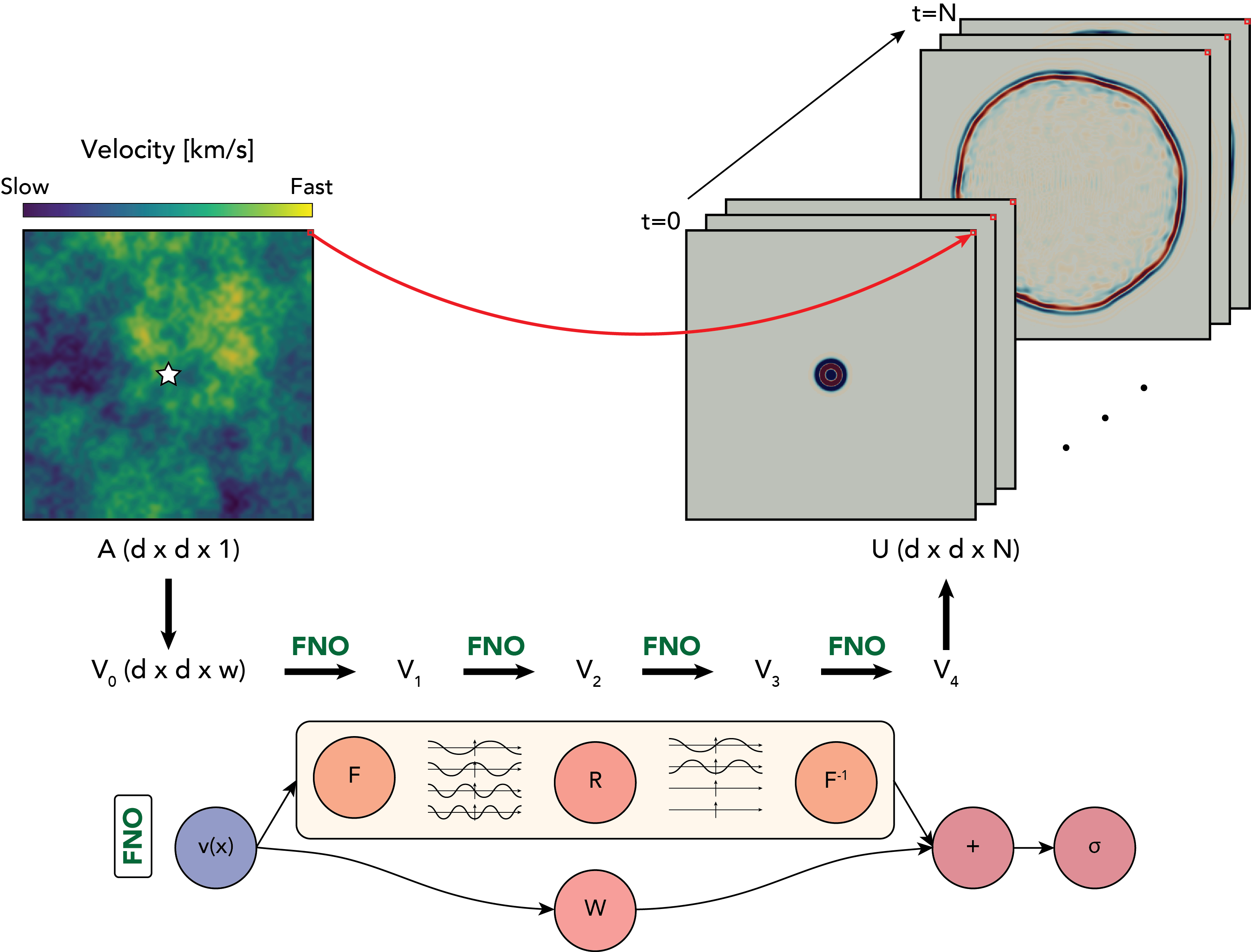
Figure 1: Our approach applying FNO to the 2D acoustic wave equation. The inputs to the FNO model are the velocity model with dimensions $d\times d\times 1$ and the source location, indicated by the white star. The input velocity model is lifted to a higher dimensional space with size $d\times d\times w$ using a neural network. Then, we apply four Fourier operator layers, and finally project back to the target wavefield dimensions of $d\times d\times N$ using a neural network. The bottom panel shows details of the Fourier layer architecture: we define $v$ to be the input. On top: We apply a Fourier transform F to $v$, then apply a linear transformation R to the lower Fourier modes, filtering out higher modes. Then we apply an inverse Fourier transform F^-1. On the bottom: we apply a local linear transform W to $v$.

4 Experiments

Initial wavefield demonstration

Figure 2 shows two example wavefields corresponding to two different velocity models, each with a different source. The spectral element solution is shown alongside the wavefield predicted by the FNO for the 8 different receivers (blue triangles). For these examples, the input velocity model is 64$\times$64. The relative $\ell_{2}$ loss of the FNO wavefields are 0.180 and 0.363. These examples are representative of the entire validation dataset, which has a loss of 0.273 relative to the spectral element solutions.

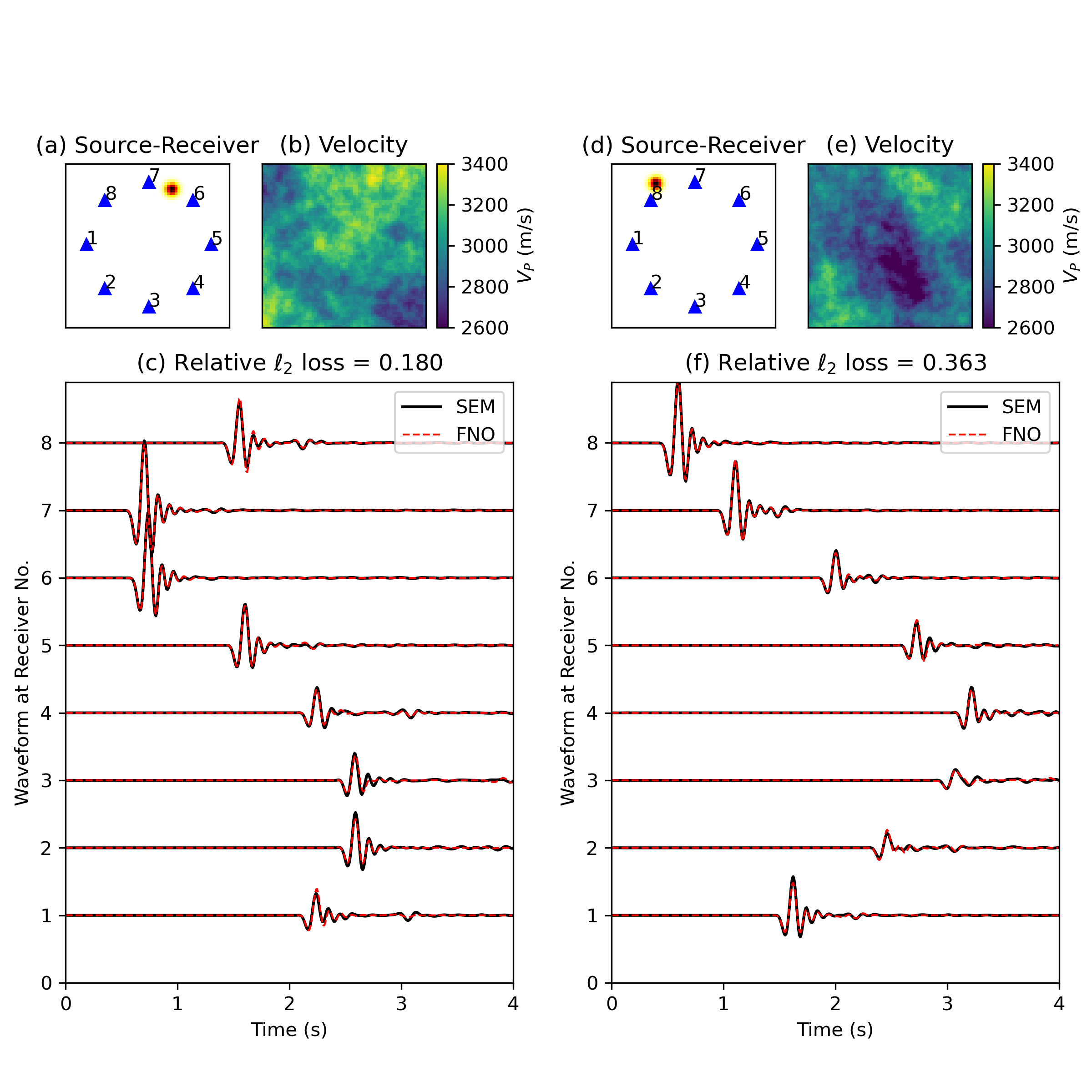
Figure 2: Examples of two validation wavefield simulations from the trained FNO model. (a) the source-receiver locations with receivers in blue and source in red; (b) the velocity structure; (c) waveforms simulated with SEM (black) and FNO (red). (d-f) same as (a-c), but for a different velocity model. The relative $\ell_{2}$ loss of the two examples are 0.180 and 0.363, respectively, which are representative of the entire validation data set with an average $\ell_{2}$ loss of 0.273. We demonstrate that the FNO simulation results are able to capture both the major arrivals as well as some reflections.

The number of simulations needed for training

Once fully trained, the FNO can evaluate a new solution in a fraction of a second, and thus the time to train the FNO will be the vast majority of the needed compute time. A primary concern about the computational demands of the FNO approach is therefore the number of simulations needed for training. Here, we examine how the number of training simulations influences the accuracy of the solution. We create a series of tests in which the number of training simulations is varied from 800 at the fewest, to 4800 at the most. The results are shown in Figure 3 where we show the FNO wavefield predictions for each dataset. Even with 1200 training samples, there is no indication that there is overfitting since the training waveform error is similar across different models (Figure 3a,b). Training using just 1200 simulations is able to predict the major arrival. Increasing number of training samples provides a better fit of the reflections (e.g. 3.2 sec in Figure 3c).

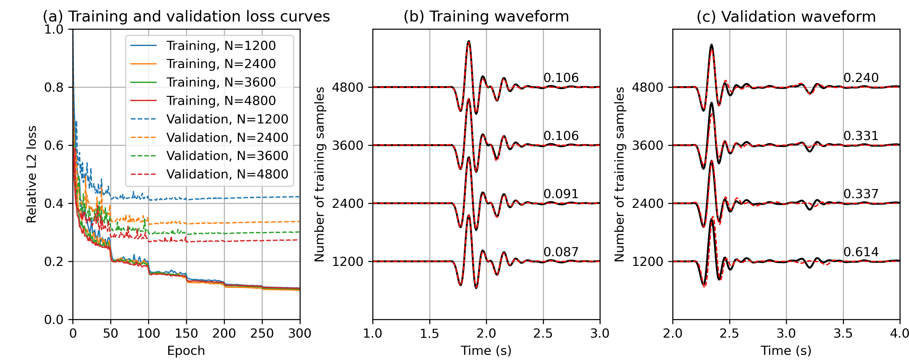
Figure 3: Model performance as a function of the number of training samples. (a) Training and validation loss curves as a function of different numbers of training samples. (b) Example waveform fitting of a single training example from models trained with varying number of training examples. (c) Example waveform fitting of a single validation example from models trained with varying number of training examples. The numbers to the right of each waveform shows the relative $\ell_{2}$ misfit. This shows that the model trained on 4800 samples is able to capture the reflections, whereas the model trained on smaller number of samples does not generalize to reflections in the validation example.

Generalization to arbitrary velocity models

The FNO was trained only on velocity models drawn from Gaussian random fields, and while this family of functions is broad, it does not include some types of functions that exist in the Earth, such as discontinuous functions. This rises the question of whether the FNO can still generalize well to these cases. Figure 4a-c shows an example of a predicted wavefield for a velocity model containing a constant velocity square embedded within a homogeneous medium. While the velocity model itself is rather simple, it is actually very far removed from the characteristics of the random fields that the FNO was trained on and represents a challenging example. We can see that the predicted wavefield does a very good job of approximating the wavefield compared to the ground truth. We believe the small residual errors can be reduced with better hyperparameter selection.

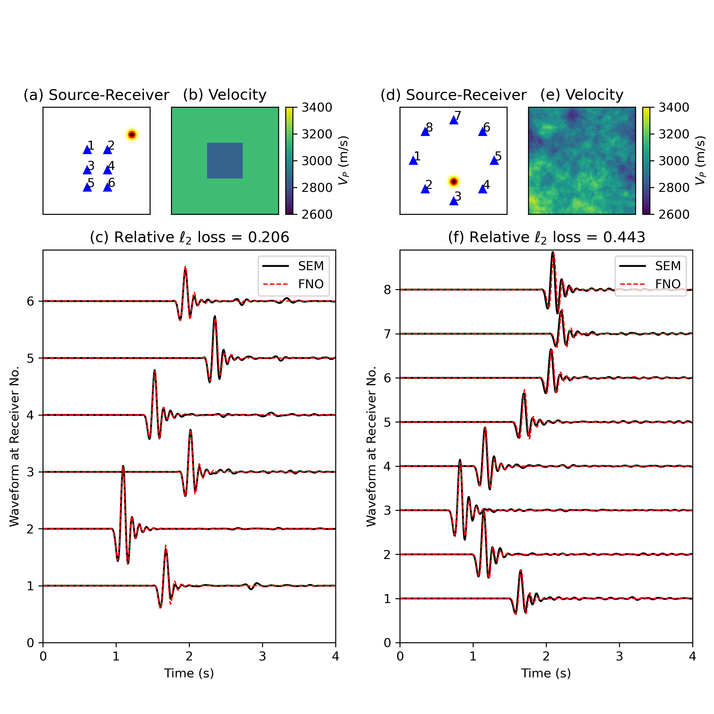
Figure 4: Model generalization experiments. (a) the source-receiver locations with receivers in blue and source in red; (b) a velocity model with a homogeneous background of 3 km/s and a 5% square anomaly; (c) waveform simulated with SEM (black) and FNO (red). (d-f) same as (a-c), but for an input velocity model with 2x finer resolution than trained on. These experiments show that the model is not just memorizing the solutions, but is able to generalize to entirely new conditions.

Generalization to higher resolution grids

FNO can be viewed in some sense as a method for learning generalized Green’s functions valid for arbitrary boundary conditions. Since it is intrinsically learning a mapping between function spaces, the FNO is theoretically independent of the resolution at which the functions are discretized (this is only a requirement for evaluation on a computer). One important advantage of this is that the FNO can be trained on velocity models with a certain grid spacing, and then be evaluated on velocity models with a different grid spacing at inference time. Here, we are not simply talking about interpolating the wavefield after solving the PDE; but rather, the solutions to the PDE can actually be evaluated on a higher resolution velocity model with negligible extra compute cost. To demonstrate this, Figure 4d-f shows the FNO prediction for a random velocity field with 2x higher resolution (128$\times$128) than the models used during training, alongside the spectral element solution. The FNO solution closely approximates the spectral element solution. Note that the velocity models with different meshes have the same roughness as the training data set. Resolving more rough structure with denser spacing can be achieved by training with many more GRFs with varying correlation length scales and variance.

Full waveform inversion with Neural Operators

One of the most useful applications of wavefield simulations is in inversion, to image the Earth’s interior. The adjoint-state method is an approach to efficiently compute the gradients of an objective function with respect to parameters of interest and can be used for seismic tomography (e.g. Tape et al., 2009; Gebraad et al., 2020). Neural Operators are differentiable by design, which enables gradient computation with reverse-mode automatic differentiation. Automatic differentiation has been shown to be mathematically equivalent to the adjoint-state method (Zhu et al., 2021). This allows for the gradients of the wavefield to be determined with respect to the inputs (velocity model and source location).

Figure 5 demonstrates our FWI performance. For each case, we compute synthetic observations using the source distribution as shown (red circles), taking every point in the 64x64 grid as a receiver. The observations are noise-free for this experiment. Then, we perform tomography by starting with a homogeneous initial velocity model and forward propagating a wavefield with the FNO for each source. We calculate the loss $L=\sum_{i}\sum_{j}[u^{obs}(x_{i},x_{j})-u^{pred}(x_{i},x_{j})]^{2}$, and compute $\nabla L$ with automatic differentiation. The velocity model is then iteratively updated with gradient descent for 1000 iterations using the Adam optimizer (Kingma and Ba, 2014) and a learning rate of 0.01. For comparison, Fig. 5ab shows the imaging result using SEM and adjoint-state method, with a relative $\ell_{2}$ misfit between the inverted and true velocity model of 0.0289. Fig. 5cd shows the result for the same velocity structure using FNO and automatic differentiation, with a misfit of 0.0319. Fig. 5ef is designed to demonstrate sharp discontinuous changes with a short wavelength. The results demonstrate the remarkable capabilities of FNO to learn a general solution operator.

We note that our FWI approach does not require an adjoint wavefield to be computed, nor a cross-correlation; the gradients can be rapidly computed with GPUs using automatic differentiation. The rapid simulation makes it substantially more efficient than adjoint methods. For these experiment, 20 sources take $\sim 1$ second for one tomographic iteration including the costs of computing the forward model, while the spectral element method with adjoint methods takes $\sim 100$ seconds for one tomographic iteration. These time measurements are from using only a single NVIDIA Tesla V100 GPU.

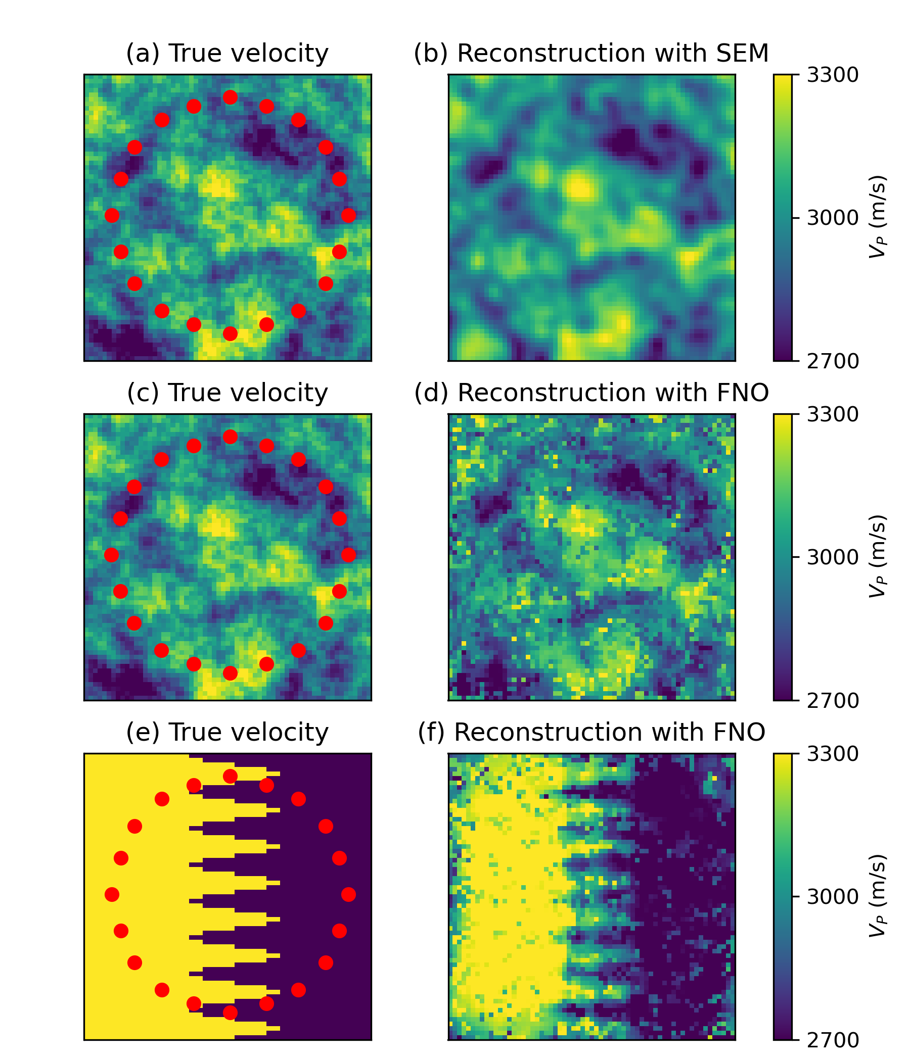
Figure 5: Example of a full waveform inversion using FNO. (a)(c)(e) True velocity models with source locations indicated by red circles and receivers placed at every node of the 64$\times$64 grid (10 km $\times$ 10 km region). (b) Reconstruction using SEM and adjoint tomography. (d)(f) Reconstruction using FNO as the forward model and automatic differentiation to compute gradients. No regularization is used for these experiments.

5 Discussion

This study presents a prototype framework for applying Neural Operators to the 2D acoustic wave equation. We anticipate that the general framework would also be suitable for the 3D elastic wave equation with relatively little modification. Indeed the FNO method was applied successfully to the Navier-Stokes equations (Li et al., 2021), which can be more challenging to solve than the elastic wave equation. In our tests, we found that only a few thousand simulations were needed to train a FNO model, and from there, required negligible time to compute a new solution. Since FNO can be trained on lower resolution simulations and then generalize to higher resolution solutions once trained, this results in substantially faster computations than using traditional numerical methods at the full resolution.

One of the limitations of the approach is that the solutions are approximate, as seen in several of the figures. However, since this is a learning-based approach, the performance can be improved in the future by using a better model architecture, thorough tuning of hyperparameters, improving the size of the training dataset, using a more appropriate objective function, and various other factors. Additionally, as new developments within machine learning emerge in this area, they would be able to be incorporated. Thus, these performance metrics should only be viewed as a starting point. For some applications, the error may be enough of an issue and traditional numerical methods may be preferable; however for many other situations in geophysics, a reasonably accurate solution may be acceptable.

Among the most exciting benefits of our approach is that by training the FNO on random velocity models, the FNO is able to produce solutions for arbitrary velocity models. This is because FNO learns a general solution operator to the PDE, and not specifically the velocity model. This means that the model does not need to be retrained for each region. Thus, the approach offers the potential for a single FNO model to be used by the entire seismology community for any region of a similar size. While the initial cost of training a FNO and performing the training simulations may be expensive, it only needs to be done a single time for the community as a whole.

References

- Afanasiev et al. (2019) Michael Afanasiev, Christian Boehm, Martin van Driel, Lion Krischer, Max Rietmann, Dave A May, Matthew G Knepley, and Andreas Fichtner. Modular and flexible spectral-element waveform modelling in two and three dimensions. Geophysical Journal International, 216(3):1675–1692, March 2019. ISSN 0956-540X. doi: 10.1093/gji/ggy469. URL https://doi.org/10.1093/gji/ggy469.
- Duputel et al. (2015) Z. Duputel, J. Jiang, R. Jolivet, M. Simons, L. Rivera, J.-P. Ampuero, B. Riel, S. E. Owen, A. W. Moore, S. V. Samsonov, F. Ortega Culaciati, and S. E. Minson. The Iquique earthquake sequence of April 2014: Bayesian modeling accounting for prediction uncertainty. Geophysical Research Letters, 42(19):7949–7957, 2015. ISSN 1944-8007. doi: 10.1002/2015GL065402. URL https://agupubs.onlinelibrary.wiley.com/doi/abs/10.1002/2015GL065402.
- Fichtner et al. (2009) Andreas Fichtner, Brian L. N. Kennett, Heiner Igel, and Hans-Peter Bunge. Full seismic waveform tomography for upper-mantle structure in the Australasian region using adjoint methods. Geophysical Journal International, 179(3):1703–1725, December 2009. ISSN 0956-540X. doi: 10.1111/j.1365-246X.2009.04368.x. URL https://doi.org/10.1111/j.1365-246X.2009.04368.x.
- Gebraad et al. (2020) Lars Gebraad, Christian Boehm, and Andreas Fichtner. Bayesian Elastic Full-Waveform Inversion Using Hamiltonian Monte Carlo. Journal of Geophysical Research: Solid Earth, 125(3):e2019JB018428, 2020. ISSN 2169-9356. doi: 10.1029/2019JB018428. URL https://agupubs.onlinelibrary.wiley.com/doi/abs/10.1029/2019JB018428. _eprint: https://agupubs.onlinelibrary.wiley.com/doi/pdf/10.1029/2019JB018428.
- Graves and Pitarka (2016) Robert Graves and Arben Pitarka. Kinematic Ground-Motion Simulations on Rough Faults Including Effects of 3D Stochastic Velocity Perturbations. Bulletin of the Seismological Society of America, 106(5):2136–2153, October 2016. ISSN 0037-1106. doi: 10.1785/0120160088. URL https://pubs.geoscienceworld.org/ssa/bssa/article/106/5/2136/350935/Kinematic-Ground-Motion-Simulations-on-Rough. Publisher: GeoScienceWorld.
- Kingma and Ba (2014) Diederik P. Kingma and Jimmy Ba. Adam: A Method for Stochastic Optimization. arXiv:1412.6980 [cs], December 2014. URL http://arxiv.org/abs/1412.6980. arXiv: 1412.6980.
- Lee et al. (2014) En-Jui Lee, Po Chen, Thomas H. Jordan, Phillip B. Maechling, Marine A. M. Denolle, and Gregory C. Beroza. Full-3-D tomography for crustal structure in Southern California based on the scattering-integral and the adjoint-wavefield methods. Journal of Geophysical Research: Solid Earth, 119(8):6421–6451, 2014. ISSN 2169-9356. doi: 10.1002/2014JB011346. URL https://agupubs.onlinelibrary.wiley.com/doi/abs/10.1002/2014JB011346. _eprint: https://agupubs.onlinelibrary.wiley.com/doi/pdf/10.1002/2014JB011346.
- Li et al. (2020a) Zongyi Li, Nikola Kovachki, Kamyar Azizzadenesheli, Burigede Liu, Kaushik Bhattacharya, Andrew Stuart, and Anima Anandkumar. Multipole Graph Neural Operator for Parametric Partial Differential Equations. arXiv:2006.09535 [cs, math, stat], October 2020a. URL http://arxiv.org/abs/2006.09535. arXiv: 2006.09535.
- Li et al. (2020b) Zongyi Li, Nikola Kovachki, Kamyar Azizzadenesheli, Burigede Liu, Kaushik Bhattacharya, Andrew Stuart, and Anima Anandkumar. Neural Operator: Graph Kernel Network for Partial Differential Equations. arXiv:2003.03485 [cs, math, stat], March 2020b. URL http://arxiv.org/abs/2003.03485. arXiv: 2003.03485.
- Li et al. (2021) Zongyi Li, Nikola Kovachki, Kamyar Azizzadenesheli, Burigede Liu, Kaushik Bhattacharya, Andrew Stuart, and Anima Anandkumar. Fourier Neural Operator for Parametric Partial Differential Equations. arXiv:2010.08895 [cs, math], May 2021. URL http://arxiv.org/abs/2010.08895. arXiv: 2010.08895.
- Moseley et al. (2020a) Ben Moseley, Andrew Markham, and Tarje Nissen-Meyer. Solving the wave equation with physics-informed deep learning. arXiv:2006.11894 [physics], June 2020a. URL http://arxiv.org/abs/2006.11894. arXiv: 2006.11894.
- Moseley et al. (2020b) Ben Moseley, Tarje Nissen-Meyer, and Andrew Markham. Deep learning for fast simulation of seismic waves in complex media. Solid Earth, 11(4):1527–1549, August 2020b. ISSN 1869-9510. doi: 10.5194/se-11-1527-2020. URL https://se.copernicus.org/articles/11/1527/2020/. Publisher: Copernicus GmbH.
- Moseley et al. (2021) Ben Moseley, Andrew Markham, and Tarje Nissen-Meyer. Finite Basis Physics-Informed Neural Networks (FBPINNs): a scalable domain decomposition approach for solving differential equations. arXiv:2107.07871 [physics], July 2021. URL http://arxiv.org/abs/2107.07871. arXiv: 2107.07871.
- Rodgers et al. (2019) Arthur J. Rodgers, N. Anders Petersson, Arben Pitarka, David B. McCallen, Bjorn Sjogreen, and Norman Abrahamson. Broadband (0–5 Hz) Fully Deterministic 3D Ground-Motion Simulations of a Magnitude 7.0 Hayward Fault Earthquake: Comparison with Empirical Ground-Motion Models and 3D Path and Site Effects from Source Normalized Intensities. Seismological Research Letters, 90(3):1268–1284, May 2019. ISSN 0895-0695. doi: 10.1785/0220180261. URL https://pubs.geoscienceworld.org/ssa/srl/article/90/3/1268/568984/Broadband-0-5-Hz-Fully-Deterministic-3D-Ground. Publisher: GeoScienceWorld.
- Smith et al. (2020) Jonathan D. Smith, Kamyar Azizzadenesheli, and Zachary E. Ross. EikoNet: Solving the Eikonal Equation With Deep Neural Networks. IEEE Transactions on Geoscience and Remote Sensing, pages 1–12, 2020. ISSN 1558-0644. doi: 10.1109/TGRS.2020.3039165. Conference Name: IEEE Transactions on Geoscience and Remote Sensing.
- Smith et al. (2021) Jonathan D. Smith, Zachary E. Ross, Kamyar Azizzadenesheli, and Jack B. Muir. HypoSVI: Hypocenter inversion with Stein variational inference and Physics Informed Neural Networks. arXiv:2101.03271 [physics], January 2021. URL http://arxiv.org/abs/2101.03271. arXiv: 2101.03271.
- Tape et al. (2009) Carl Tape, Qinya Liu, Alessia Maggi, and Jeroen Tromp. Adjoint Tomography of the Southern California Crust. Science, 325(5943):988–992, August 2009. ISSN 0036-8075, 1095-9203. doi: 10.1126/science.1175298. URL https://science.sciencemag.org/content/325/5943/988. Publisher: American Association for the Advancement of Science Section: Report.
- Virieux and Operto (2009) J. Virieux and S. Operto. An overview of full-waveform inversion in exploration geophysics. GEOPHYSICS, 74(6):WCC1–WCC26, November 2009. ISSN 0016-8033. doi: 10.1190/1.3238367. URL https://library.seg.org/doi/full/10.1190/1.3238367. Publisher: Society of Exploration Geophysicists.
- Wang and Zhan (2020) Xin Wang and Zhongwen Zhan. Moving from 1-D to 3-D velocity model: automated waveform-based earthquake moment tensor inversion in the Los Angeles region. Geophysical Journal International, 220(1):218–234, January 2020. ISSN 0956-540X. doi: 10.1093/gji/ggz435. URL https://doi.org/10.1093/gji/ggz435.
- Xiao et al. (2021) Cong Xiao, Ya Deng, and Guangdong Wang. Deep-Learning-Based Adjoint State Method: Methodology and Preliminary Application to Inverse Modeling. Water Resources Research, 57(2):e2020WR027400, 2021. ISSN 1944-7973. doi: 10.1029/2020WR027400. URL https://agupubs.onlinelibrary.wiley.com/doi/abs/10.1029/2020WR027400. _eprint: https://agupubs.onlinelibrary.wiley.com/doi/pdf/10.1029/2020WR027400.
- Ye et al. (2016) Lingling Ye, Thorne Lay, Hiroo Kanamori, and Luis Rivera. Rupture characteristics of major and great mw 7.0 megathrust earthquakes from 1990 to 2015: 2. Depth dependence. Journal of Geophysical Research: Solid Earth, 121(2):2015JB012427, February 2016. ISSN 2169-9356. doi: 10.1002/2015JB012427. URL http://onlinelibrary.wiley.com/doi/10.1002/2015JB012427/abstract.
- Zhang and Gao (2021) Wei Zhang and Jinghuai Gao. Deep-Learning Full-Waveform Inversion Using Seismic Migration Images. IEEE Transactions on Geoscience and Remote Sensing, pages 1–18, 2021. ISSN 1558-0644. doi: 10.1109/TGRS.2021.3062688. Conference Name: IEEE Transactions on Geoscience and Remote Sensing.
- Zhu et al. (2020) Weiqiang Zhu, Kailai Xu, Eric Darve, Biondo Biondi, and Gregory C. Beroza. Integrating Deep Neural Networks with Full-waveform Inversion: Reparametrization, Regularization, and Uncertainty Quantification. arXiv:2012.11149 [physics], December 2020. URL http://arxiv.org/abs/2012.11149. arXiv: 2012.11149.
- Zhu et al. (2021) Weiqiang Zhu, Kailai Xu, Eric Darve, and Gregory C Beroza. A general approach to seismic inversion with automatic differentiation. Computers & Geosciences, 151:104751, 2021.