Multi-epoch searches for relativistic binary pulsars and fast transients in the Galactic Centre

Abstract

The high stellar density in the central parsecs around the Galactic Centre makes it a seemingly favourable environment for finding relativistic binary pulsars. These include pulsars orbiting other neutron stars, stellar-mass black holes or the central supermassive black hole, Sagittarius A*. Here we present multi-epoch pulsar searches of the Galactic Centre at four observing frequencies, $(4.85,\,8.35,\,14.6,\,18.95)\,{\rm GHz}$, using the Effelsberg 100-m radio telescope. Observations were conducted one year prior to the discovery of, and during monitoring observations of, the Galactic Centre magnetar PSR J1745$-$2900. Our data analysis features acceleration searches on progressively shorter time series to maintain sensitivity to relativistic binary pulsars. The multi-epoch observations increase the likelihood of discovering transient or nulling pulsars, or ensure orbital phases are observed at which acceleration search methods work optimally. In $\sim 147\,{\rm h}$ of separate observations, no previously undiscovered pulsars have been detected. Through calibration observations, we conclude this might be due to insufficient instantaneous sensitivity; caused by the intense continuum emission from the Galactic Centre, its large distance and, at higher frequencies, the aggregate effect of steep pulsar spectral indices and atmospheric contributions to the system temperature. Additionally we find that for millisecond pulsars in wide circular orbits $(\lesssim 800\,{\rm d})$ around Sagittarius A*, linear acceleration effects cannot be corrected in deep observations $(9\,{\rm h})$ with existing software tools. Pulsar searches of the Galactic Centre with the next generation of radio telescopes $-$ such as MeerKat, ngVLA and SKA1-mid $-$ will have improved chances of uncovering this elusive population.

1 Introduction

Binary radio pulsars are precision tools for tests of gravitational theories in the strong field regime (see e.g. Wex, 2014, for a review of key results). In general, the larger the mass of the pulsar companion, and the more compact and eccentric its orbit, increased is the extent and precision to which gravity tests can be performed. For this reason, the Galactic Centre (GC) is a tantalizing target for pulsar searches. In addition to having the highest stellar density in the Galaxy, it hosts the massive compact object, Sagittarius A* (hereafter Sgr A*), which is shown to be a supermassive black hole (SMBH). With a mass of approximately $4\times 10^{6}\,$${\rm M}_{\odot}\;$and a distance just over $\rm{8\,kpc}$ (Eckart & Genzel, 1996; Ghez et al., 2008; Gillessen et al., 2009; Gravity Collaboration et al., 2019) it is Earth’s nearest SMBH and offers a unique opportunity to test the General Theory of Relativity (GR) and the base properties of black holes via astrometry of orbiting stars (Gravity Collaboration et al., 2018; Do et al., 2019) and direct VLBI imaging at mm-wavelengths (Event Horizon Telescope Collaboration et al., 2019). The detection of even a “typical” pulsar (spin period, $P\sim 0.5\,{\rm s}$) in an orbit around Sgr A*, of the order of years, can enable tests of the Cosmic Censorship Conjecture and the No Hair Theorem; two of the most fundamental predictions of GR (Wex & Kopeikin, 1999; Kramer et al., 2004; Liu et al., 2012; Liu & Eatough, 2017). When combined with stellar astrometry and imaging, results from a pulsar experiment are highly complementary and will help to build a complete description of Sgr A* (Psaltis et al., 2016).

Multi-wavelength observations of the GC indicate that the number of pulsars in the central few parsecs should be high (Wharton et al., 2012) and conditions are highly favourable for relativistic binaries (Faucher-Giguère & Loeb, 2011). The dense nuclear star cluster surrounding Sgr A* (see e.g. Genzel et al., 2010, for a review) contains a majority of older late-type stars, but contrary to expectations, massive young main-sequence stars (Ghez et al., 2003) and possible neutron star progenitors such as Wolf-Rayet stars (Paumard et al., 2001). The presence of neutron stars is further indicated by large numbers of X-ray binaries, possible pulsar wind nebulae, X-ray features like the “cannonball” and compact radio variables (Muno et al., 2005; Wang et al., 2006; Zhao et al., 2013, 2020). Despite this only six radio pulsars have been discovered within half a degree of Sgr A* (Johnston et al., 2006; Deneva et al., 2009; Eatough et al., 2013c; Shannon & Johnston, 2013) even after many dedicated searches at multiple wavelengths (Kramer et al., 1996a, 2000; Klein et al., 2004; Klein, 2005; Deneva, 2010; Macquart et al., 2010; Siemion et al., 2013; Eatough et al., 2013a). Hyperstrong scattering of radio waves in the GC has been the principal explanation for the scarcity of detected pulsars (Cordes & Lazio, 1997a; Lazio & Cordes, 1998a, b; Cordes & Lazio, 2002), however, scatter broadening measurements of PSR J1745$-$2900 in Spitler et al. (2014) and Bower et al. (2014) appear to contest this. Other authors have noted that the lack of GC pulsars is expected under a certain set of conditions and considering the sensitivity limits of existing pulsar surveys (Chennamangalam & Lorimer, 2014; Rajwade et al., 2017; Liu & Eatough, 2017). Alternatively, the scarcity of detected pulsars might be caused by a more complex scattering structure toward the GC (Cordes & Lazio, 1997b; Lazio & Cordes, 1998a, b; Johnston et al., 2006; Schnitzeler et al., 2016; Dexter et al., 2017).

In this work we have tackled additional and necessary requirements for pulsar searches of the GC that have thus far not been fully addressed. These include: a) repeated high frequency $(\gtrsim 5\,{\rm GHz})$ observations over a long duration $(\mathcal{O}\,{\rm yr})$; b) analysis of all observations with binary pulsar search algorithms capable of detecting pulsars in binary systems with a wide range of orbital periods; c) searches for bright single pulse emission from fast transient sources. The following is a brief outline of the rest of this paper. In Section 2 the observations, data processing and measurements of the observational system sensitivity are described. In Section 3 the basic results of this search are given. Section 4 provides discussion of our results in the context of previous pulsar searches of the GC and remaining shortcomings. We also discuss the prospects for future searches of the GC with current and next generation radio telescopes. Section 6 presents a summary.

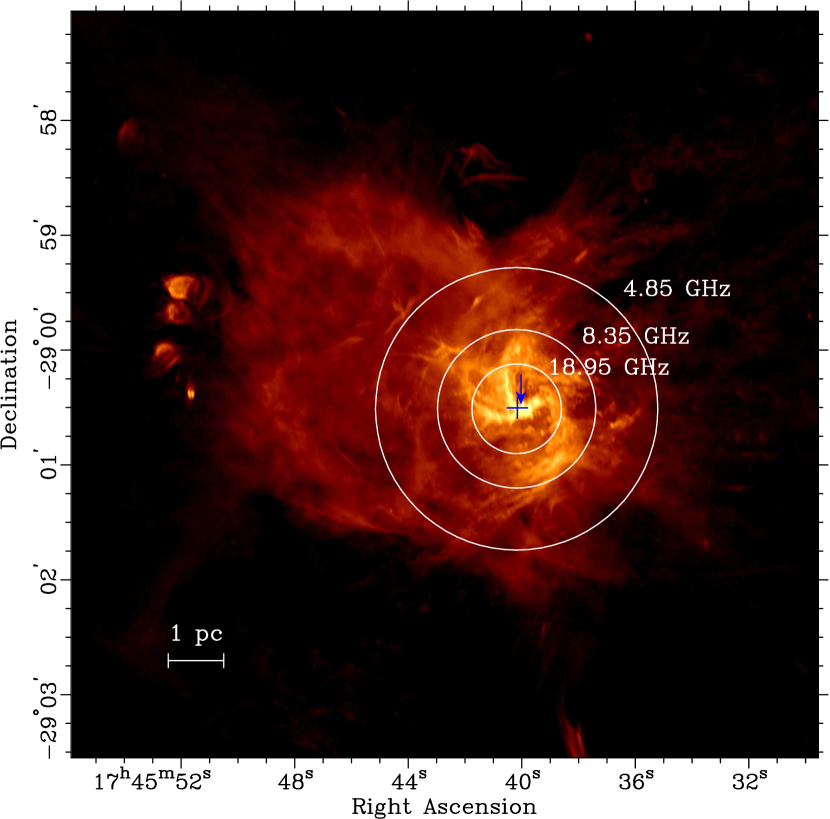
Figure 1: The areas covered by our search at three observing frequencies as indicated by the relevant HPBW overlaid on a 5.5 GHz Jansky VLA map of the Sgr A complex from Zhao et al. (2016). The HPBW at 14.6 GHz is only 10 per cent larger than that at 18.95 GHz, so has not been plotted for clarity. The blue cross marks the position of PSR J1745$-$2900 and the location of Sgr A* is indicated by the blue vertical arrow in the top right quadrant of the cross. A physical scale of 1 pc is indicated in the bottom left using a recently derived geometric GC distance (Gravity Collaboration et al., 2019).

2 Observations, Data Processing and System Sensitivity

2.1 Observations

Observations were made with the Effelsberg 100-m radio telescope, of the Max Planck Institute for Radio Astronomy, between February 2012 and February 2016. In 2012 all data were taken at 18.95 GHz and targeted the position of Sgr A* ($\rm{RA_{J2000}=17^{\rm h}\,45^{\rm m}\,40^{\rm s}.0409}$, $\rm{Dec_{J2000}=-29^{\circ}\,00\arcmin\,28\arcsec.118}$; Reid & Brunthaler 2004), as part of a ‘stack search’ for solitary pulsars (Eatough et al., 2013a). After the discovery of radio pulsations from the GC magnetar PSR J1745$-$2900 in April 2013 (Eatough et al., 2013c; Shannon & Johnston, 2013), a multi-frequency monitoring program of this object was started (see Desvignes et al., 2018, for details of this campaign). Pulsar search-mode observations were performed in parallel with timing observations of PSR J1745$-$2900 that were folded with a contemporaneous ephemeris. All observations were centred on the X-ray position of PSR J1745$-$2900 as measured with the Chandra observatory ($\rm{RA_{J2000}=17^{\rm h}\,45^{\rm m}\,40^{\rm s}.2}$, $\rm{Dec_{J2000}=-29^{\circ}\,00\arcmin\,30\arcsec.4;}$ Rea et al., 2013), 2.4$\arcsec$ away from Sgr A*. Receivers with central frequencies, $\nu$, of $(4.85,\,8.35,\,14.60,\,18.95)\,{\rm GHz}$, and respective half-power beam widths (HPBW) of 146$\arcsec$ (5.8 pc), 82$\arcsec$ (3.3 pc), 51$\arcsec$ (2.0 pc) and 46$\arcsec$ (1.8 pc) $-$ where the corresponding physical scale at the distance of the GC is indicated in brackets $-$ were used (see Figure 1). At all frequencies both PSR J1745$-$2900 and Sgr A* are within the HPBW and any reduction in sensitivity toward Sgr A* due to offset pointing was negligible.

The search-mode data $-$ a digital filterbank with bandwidth 500 MHz, 128 spectral channels and a sampling interval of 65.536 $\mu$s $-$ were recorded with the Pulsar Fast-Fourier-Transform Spectrometer (PFFTS) backend at the three lowest frequencies. At 18.95 GHz the X-Fast-Fourier-Transform Spectrometer (XFFTS) was used to cover the larger available bandwidth of 2 GHz. Here each linear polarization was sampled independently with an interval of 128 $\mu$s across 256 spectral channels. After acquisition, the two polarisations were combined offline. Data from both backends originally consisted of 32-bit integer samples for each frequency channel in a bespoke data format. This was converted to sigproc filterbank format along with downconversion to 8-bit samples performed by a dedicated C++ program.

In this work, 112 independent epochs (or $\sim$147 h) of GC observations have been taken and analyzed. The maximum duration of an individual observation was 2.4 h, which is the total time the Sgr A* region is visible from Effelsberg each day. The benefits of our repetitive observational scheme is manifold. Binary pulsars can be “hidden” by transient phenomena such as relativistic spin-precession (e.g. Kramer, 1998; Breton et al., 2008; Desvignes et al., 2019), binary eclipses (e.g. Johnston et al., 1992; Freire, 2005) and sub-optimal orbital phases for acceleration search algorithms (Eatough et al., 2013b). In addition, both solitary and binary pulsars can exhibit burst-like or transient emission in the form of giant pulses (e.g. Jessner et al., 2005), nulling or intermittent pulsations (Kramer et al., 2006a; Knispel et al., 2013). These effects can make it impossible to detect certain pulsars in just a single survey observation.

2.2 Data processing

The data were processed using the Max-Planck-Gesellschaft Supercomputer HYDRA with a pulsar searching pipeline utilizing the presto software package (Ransom, 2001). A basic outline of the search pipeline is as follows.

Firstly, because pulse broadening caused by scattering toward the GC (Spitler et al., 2014) made the original sampling interval unnecessarily fine, data at 4.85 GHz and 8.35 GHz were down-sampled in time, with a dedicated python script, by a factor of four and two respectively; thereby reducing the computational requirements. At the higher frequencies of $14.6\,{\rm GHz}$ and $18.95\,{\rm GHz}$, where scatter broadening is smaller, no down-sampling was performed.

Table 1: Details of the data configuration and searching parameters used at each central observing frequency, $\nu$. $\rm{\Delta\nu}$ is the total bandwidth, $n_{\rm c}$ is the number of frequency channels, $T_{\rm obs}$ is the total integration length, $\tau$ is the sampling time, $\Delta{\rm DM}$ is the range of dispersion measures explored, $n_{\rm seg}$ is the number of consecutive segments of the original integration analyzed in the acceleration search, viz. $2^{0}$ corresponds to one segment of the full integration length $T_{\rm obs}$, $2^{1}$ corresponds to two consecutive segments of length $T_{\rm obs}/2$ and so forth. At all frequencies and in all segments the $z_{\rm max}$ parameter, which denotes the maximum number of Fourier bin drifts searched in the presto routine accelsearch, was set to $z_{\rm max}=1200$.

$\nu$	$\rm{\Delta\nu}$	$n_{\rm c}$	$T_{\rm obs}$	$\tau$	$\Delta{\rm DM}$	$n_{\rm seg}$
(GHz)	(GHz)		(hr)	($\rm{\mu s}$)	($\rm{cm^{-3}\,pc}$)
$\rm{4.85}$	0.5	128	1.2	262.1	$800$-$11,900$	$2^{0}$-$2^{4}$
$\rm{8.35}$	0.5	128	2.4	131.1	$800$-$15,080$	$2^{0}$-$2^{5}$
$\rm{14.60}$	0.5	128	1.2	65.5	$800$-$10,800$	$2^{0}$-$2^{4}$
$\rm{18.95}$	2.0	256	2.4	128.0	$800$-$21,200$	$2^{0}$-$2^{5}$

Next the data from an individual observation (typically of length $\rm{\sim 1.2\,h}$ or $\rm{\sim 2.4\,h}$) was recursively split into segments of half the observing duration, $T_{\rm obs}$, down to a minimum segment length of $\simeq 4.5\,{\rm min}$. Segmentation of the data is performed in order to maintain sensitivity to pulsars in shorter orbital period systems using so-called “constant acceleration searches” that are most effective when $T_{\rm obs}\lesssim P_{\rm b}/10$, where $P_{\rm b}$ is the orbital period (Ransom et al., 2003; Ng et al., 2015). Such segmented acceleration search schemes have been employed in a re-analysis of the Parkes multi-beam pulsar survey (Eatough et al., 2013b), and to the low Galactic latitude region of the High-Time-Resolution-Universe South survey (Ng et al., 2015), discovering the most highly accelerated pulsar currently known (Cameron et al., 2018). From the relation described above, our minimum segment length of $\simeq 4.5\,{\rm min}$ results in a minimum detectable orbital period of $\simeq 45\,{\rm min}$. However, segmentation of data to improve binary search sensitivity is a trade-off with the intrinsic sensitivity, defined by the minimum detectable flux density, $S_{\rm min}$, which is $\propto\,\sqrt{T_{\rm obs}}$ (see Section 2.3 for more details of the sensitivity of the observing system used here). Hereafter $T_{\rm obs}$ can refer to the duration of the original observation, or the length of an individual data segment.

After segmentation, the detrimental effects of Radio Frequency Interference (RFI) were mitigated with the presto routine rfifind and a list of periodic signals to be excluded from further analysis. This list includes the domestic mains power, at frequency 50 Hz with a number of its harmonics, and the first 32 integer harmonics of PSR J1745$-$2900 which is prevalent throughout the observations after April 28^th 2013. The data were then transformed into the inertial reference frame of the solar system barycentre and dedispersed to time series assuming different dispersive delays, starting at a trial dispersion measure (DM) of 800$\rm\,cm^{-3}\,pc$ based on the DM of known pulsars in the GC, with the largest trial DM value and the number and size of the DM steps dependent on the frequency, bandwidth and sampling interval of the observation as determined by the presto routine ddplan.py. For a DM of 800$\rm\,cm^{-3}\,pc$ (equivalent to our lowest choice of trial DM) intra-channel dispersion smearing at the lower frequency edge of the band is $266$ and $49\,\mu{\rm s}$ at $4.85$ and $8.35\,{\rm GHz}$ respectively. This corresponds to $1.01\tau$ and $0.19\tau$, where $\tau$ is the sampling time, at $4.85$ and $8.35\,{\rm GHz}$ respectively. Neglecting pulse scattering (which could be the dominant effect in this direction), a marginal reduction in sensitivity to MSPs might therefore be expected at $8.35\,{\rm GHz}$. Details of the various observational configurations and data processing parameters used are summarised in Table 1.

A search for single pulses from fast transient sources was performed on the longest available dedispersed time series using single_pulse_search.py from presto. Box-car filters with widths up to $150\tau$ were used to record events with intensity $\geq 6\,\sigma$ (see Karako-Argaman et al., 2015, e.g. for details on single pulse searches). The dedispersed time series were then corrected for red noise effects and searched for periodic (and accelerated) signals with the presto program accelsearch. The line-of-sight (l.o.s) acceleration caused by a binary companion, $a$, makes the spin frequency, $f$, of a pulsar drift in the Fourier spectrum by a number of spectral bins, $n_{\rm drift}$, given by $n_{\rm drift}=af{T_{\rm obs}}^{2}/c$, where $T_{\rm obs}$ is the integration length and $c$ is the speed of light. accelsearch uses the ‘correlation technique’ to collect the smeared signal back into a single spectral bin by the application of Fourier domain matched filtering; in practice by convolution of a small range of Fourier bins, around the relevant spectral bin, with the complex conjugated and frequency reversed version of the finite impulse response (FIR) filter that describes the signal smearing (Ransom et al., 2002; Dimoudi et al., 2018). The acceleration search, which dominated the data processing time, was performed with the Graphical Processing Unit (GPU) enabled version of the accelsearch routine. For all segment lengths the maximum value of $n_{\rm drift}$ searched (given by the accelsearch input parameter $z_{\rm max}$) was $z_{\rm max}=1200$. At this stage harmonic summing was also applied, with up to 16 harmonics summed for non-accelerated signals, and up to 8 harmonics for highly accelerated signals.

Results from the periodicity and acceleration searches were consolidated with the presto routine, accel_sift.py, to leave only detection with a harmonically summed power $\geq 6\,\sigma$; removing in the process duplicated (i.e. detected at different DMs and accelerations) and harmonically related signals. Given our choice of threshold (bespoke to these data), typically $\gtrsim 100$ candidates per segment were then folded with presto prepfold to create candidate evaluation plots. Lastly, visual inspection of these candidates was done manually via interactive scatter diagrams and/or automatically utilizing PICS AI and PEACE (Zhu et al., 2014; Lee et al., 2013).

2.3 System Sensitivity

Table 2: System sensitivity measurements $-$ indicated by $T_{\rm sys}-$ at all observing frequencies (first column) and on three sky positions described in Section 2.3 (third, fourth and fifth columns). The various contributions to $T_{\rm sys}$ from the GC, $T_{\rm GC}$, elevation dependent ground spillover and atmospheric effects, $T_{\rm elv}$, and the receiver, $T_{\rm rec}$, are indicated in the sixth, seventh and eighth columns respectively. Errors given in brackets are derived from the standard deviation of measurements over one year at $4.85\,{\rm GHz}$ and $8.35\,{\rm GHz}$, and from the standard deviation of measurements of $T_{\rm sys}$ in the first 60 individual frequency channels at $14.6\,{\rm GHz}$. The origin of figures given at $18.95\,{\rm GHz}$, where calibration was not done, are described in Section 2.3. Values of the telescope gain, receiver temperature measured at the zenith angle, $T^{\dagger}_{\rm{rec}}$, and the $\sigma_{\rm min}=10$ minimum detectable flux density (assuming a pulse width of $0.05P$ and maximum $T_{\rm obs}$ as given in Table 1) in the Sgr A* ON position, $S_{\rm min}$, are given in the second, ninth and tenth columns respectively.

		Sgr A* ON	Sgr A* OFF	NGC7027 OFF					Sgr A* ON
$\nu\,{\rm(GHz)}$	$G\,({\rm K\,Jy^{-1}})$	$T_{\rm{sys}}\,{\rm(K)}$	$T_{\rm{sys}}$ (K)	$T_{\rm{sys}}$ (K)	$T_{\rm{GC}}$ (K)	$T_{\rm{elv}}$(K)	$T_{\rm{rec}}$(K)	$T^{\dagger}_{\rm{rec}}$(K)	$S_{\rm min}$(mJy)
4.85	1.55	200(16)	63(3)	31(3)	137(16)	32(4)	31(3)	27	$0.14$
8.35	1.35	126(23)	72(15)	31(8)	55(27)	41(17)	31(8)	22	$0.07$
14.60	1.14	194(16)	155(13)	149(12)	39(21)	6(18)	149(12)	99	$0.19$
18.95	1.03	$\sim$ 124	$-$	$\sim$ 104	$20$	$-$	$\sim$ 104	64	0.05

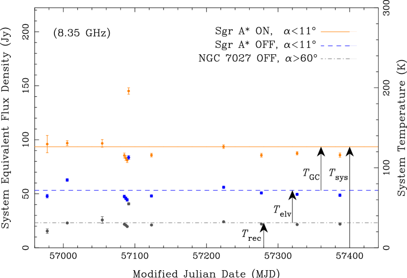
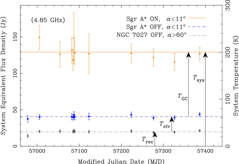
Figure 2: Observing system sensitivity $-$ quantified by the system temperature $T_{\rm sys}$, or the system equivalent flux density $S_{\rm sys}=T_{\rm sys}/G\;-$ over the course of one year of observations at Effelsberg. The top panel shows values measured at $8.35\,{\rm GHz}$ while the bottom panel shows those at $4.85\,{\rm GHz}$. Orange points indicate measurements toward Sgr A^∗; blue points are values measured at an equivalent telescope elevation as Sgr A$*$ ($\alpha<11^{\circ}$) but ‘off-source’ and black points show measurements at high telescope elevation ($\alpha>60^{\circ}$). Error bars are given from the standard deviation of values across all channels in the observing band, and solid or dashed horizontal lines show the average values.

To calculate flux density or luminosity limits of the searches presented in this work, and to establish the major contributing factors to reductions in the sensitivity of our observing system, we have calibrated the sensitivity at the three lowest frequencies. In all cases the planetary nebula ${\rm NGC}\,7027$, with a known radio spectrum (Zijlstra et al., 2008), was used as a reference source and calibration was performed with the psrchive software package. At 18.95 GHz no calibration observations were performed and the sensitivity was estimated from published system parameters.

From the radiometer equation, as applied to observations of pulsars, the limiting flux density, $S_{\rm min}\,({\rm mJy})$, of a pulsar search observation can be written

$$S_{\mathrm{min}}=\beta\frac{{\sigma_{\rm min}}\,T_{\rm sys}}{G\sqrt{n_{\mathrm{p}}\,T_{\mathrm{obs}}\,B}}\sqrt{\frac{W}{P-W}},$$ (1)

where $\beta$ accounts for digitisation losses and is negligible $(\beta\simeq 1)$ for 8-bit sampling, $G\,({\rm K\,Jy}^{-1})$ is the telescope gain, ${\sigma_{\rm min}}$ is the minimum statistically detectable signal to noise ratio, $n_{\rm p}$ is the number of polarisations summed, $B\,({\rm MHz})$ is the receiver bandwidth and $P$ and $W$ are the pulse period and width respectively. $T_{\rm sys}\,({\rm K})$ is the system temperature given by

$$T_{\rm sys}=T_{\rm rec}+T_{\rm sky}+T_{\rm atm}+T_{\rm elv}.$$ (2)

Here $T_{\rm rec}$ is the instrumental receiver noise temperature, $T_{\rm sky}$ is the astrophysical background sky temperature, $T_{\rm atm}$ is the combined effects of atmospheric opacity and water vapour emission (centred around $\sim 22\,{\rm GHz}$) and $T_{\rm elv}$ is the elevation dependent blackbody spillover radiation from the ground combined with an increased column depth of atmosphere. As noted by Johnston et al. (2006) and Macquart et al. (2010), at frequencies $\lesssim 8\,{\rm GHz}$, $T_{\rm sky}$ has a significant impact on the sensitivity of GC pulsar searches because continuum emission in the GC $-$ from a combination of thermal and nonthermal sources $-$ is known to be exceptionally bright: $T_{\rm sky}\sim T_{\rm GC}\simeq\mathcal{O}100\,{\rm K}$ (e.g. Pedlar et al., 1989; Reich et al., 1990; Law et al., 2008). At frequencies $\gtrsim 15\,{\rm GHz}$, atmospheric and elevation dependent spillover effects are thought to become the dominant contributors to $T_{\rm sys}$ (Macquart et al., 2010).

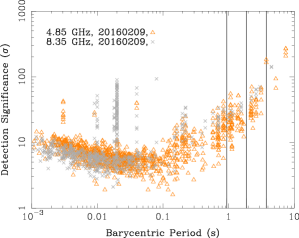
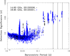
Figure 3: Scatter diagrams showing the barycentric pulse period versus folded detection significance of pulsar candidates generated from the periodicity search of four individual epochs (dates in legend) at different observing frequencies. Each point represents a pulsar candidate that was inspected either by eye and/or with machine learning tools. The upper panel shows results from searches at $4.85\,{\rm GHz}$ and $8.35\,{\rm GHz}$ and the lower panel those at $14.6\,{\rm GHz}$ and $18.95\,{\rm GHz}$. The solid vertical lines indicate the barycentric spin period of PSR J1745$-$2900 and subsequent harmonics at one half and one quarter of the fundamental spin period.

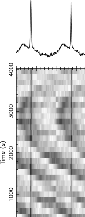
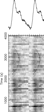
Figure 4: Example presto prepfold folded profiles from the periodicity search at $4.85\,{\rm GHz}$ showing a detection of PSR J1745$-$2900 and the anomalously drifting signal described in Section 3.1 (left-hand panels). In the right-hand panels the same data are re-folded with an optimum $P,\,\dot{P}$ and $\ddot{P}$ to recover the anomalously drifting signal. The lower panels show folded subintegrations throughout the observation duration, while the upper panels show the folded and fully integrated pulse profile.

By using $T_{\rm sys}$, or the corresponding system equivalent flux density $S_{\rm sys}=T_{\rm sys}/G\,({\rm Jy})$, as a useful marker of the instantaneous sensitivity of our observing system, the effects described above have been investigated. Values of $T_{\rm sys}$ at three pertinent sky positions were measured: directly toward Sgr A* (labeled Sgr A* ON); at the same telescope elevation, $\alpha$, as Sgr A* $(\alpha<11^{\circ})$, but off source (Sgr A* OFF); and at high telescope elevation $(\alpha>60^{\circ})$ close to the calibrator ${\rm NGC}\,7027$ but also off source (${\rm NGC}\,7027$ OFF). Results of this analysis can be seen in Figure 2, where the measurements of $T_{\rm sys}$ at $4.85\,{\rm GHz}$ and $8.35\,{\rm GHz}$ over the course of one year of observations is plotted. Average values of $T_{\rm sys}$, and flux density limits, at all frequencies are also given in Table 2. From simple differencing we are able to investigate the relative contributions of $T_{\rm GC}$, $T_{\rm elv}$ and $T_{\rm rec}$. At $4.85\,{\rm GHz}$, $T_{\rm GC}\sim 140\,{\rm K}$ and is the largest contributor to $T_{\rm sys}$, whereas at $8.35\,{\rm GHz}$ $T_{\rm GC}\sim 55\,{\rm K}$ which is less than the combined effect of $T_{\rm elv}$ and $T_{\rm rec}$ at this frequency. In all of our measurements $T_{\rm atm}$ is degenerate with values of $T_{\rm rec}$, however by comparison with values of the system temperature measured at the zenith angle, and corrected for opacity effects, (denoted $T^{\dagger}_{\rm{rec}}$ in Table 2) we can estimate the contribution from $T_{\rm atm}$ close to zenith. At $14.6\,{\rm GHz}$ $T_{\rm atm}\sim 50\,{\rm K}$ which is the largest amongst our calibrated values. At frequencies in the K-band $(18-27\,{\rm GHz})$ $T_{\rm atm}$ can vary by factors of a few depending upon the weather (Roy et al., 2004). Therefore, observations at $18.95\,{\rm GHz}$ were always performed in wintertime and under ideal weather conditions. $T_{\rm sys}$ in the Sgr A* ON position was conservatively estimated using the measured value of $T_{\rm rec}=64\,{\rm K}$, $T_{\rm atm}\sim 40\,{\rm K}$ - from the good weather conditions displayed in Figure 5. of Roy et al. (2004) and $T_{\rm GC}=20\,{\rm K}$ - by fitting a power law spectrum to the three lower frequency $T_{\rm GC}$ measurements (resulting spectral index of $-1.4\pm 0.3$). The derived value of $T_{\rm sys}$ in the Sgr A* ON position comes to $124\,{\rm K}$. From test observations of PSR B2020+28, with known flux density at this frequency (Kramer et al., 1996b), and utilizing Equation 1, we find agreement on this value of $T_{\rm sys}$ to within a factor of two.

At the two lowest frequencies, system temperature measurements are typically stable for all telescope orientations and observing epochs over the course of one year, with the exception of a period around MJD 57080 at $8.35\,$GHz where a jump in $T_{\rm sys}$ is observed for all telescope orientations. This might be attributed to adverse weather conditions, or heightened levels of RFI on this day. All sensitivity measurements with the PFFTS and XFFTS backends presented in this section were consistent to the ten per cent level with those from commensal observations using the PSRIX backend (Desvignes et al., 2018; Lazarus et al., 2016).

3 Results

Figure 5: Example presto single_pulse_search.py diagnostic plot from our transient search showing a detection of single pulses from PSR J1745$-$2900. Starting at the top left-hand panel and moving clockwise, the candidate plot shows; a histogram number of pulses as a function of pulse detection ${\rm S/N}$; a histogram of the number of pulses as a function of dispersion measure; a scatter diagram of the pulse ${\rm S/N}$ as a function of dispersion measure; a scatter diagram showing pulses as a function of dispersion measure and time through the observation - the size of a point is indicative of its ${\rm S/N}$. At the top, various observational diagnostics are given in plain text.

At the time of writing, no undiscovered pulsars or transients have been detected. Scatter diagrams showing example results from the periodicity search of individual epochs at each observing frequency can be seen in Figure 3. Such scatter diagrams were used to quickly select and display candidate detection diagnostics (presto prepfold plots) of any promising pulsar candidates. For this task the so-called combustible-lemon software tool was used. Typically up to $\sim 19,000$ candidates could be generated for each observing epoch. As is typical in these scatter diagrams, repeated detections of the same periodicity in independent observations, or data segments, are visible as “columns” (Faulkner et al., 2004; Keith et al., 2009). Whereas these can normally be attributed to terrestrial RFI detected at multiple sky locations our segmented acceleration search algorithm, applied to a single position on the sky, could also create detection “columns” for genuine pulsar signals.

Despite masking of its fundamental spin frequency and the first 32 integer harmonics, PSR J1745$-$2900 was found in the periodicity search results of multiple epochs at $4.85$ and $8.35\,{\rm GHz}$; typically via fractional harmonics of the fundamental spin frequency (see Figure 3, upper panel). The upper panel of Figure 3 shows $4.85\,{\rm GHz}$ results data from February $9^{\rm th}$ 2016 where two detections of PSR J1745$-$2900 can be seen at the fundamental spin period in addition to multiple detection columns at shorter periods due to RFI. The corresponding presto prepfold pulse profile is shown in the left hand panel of Figure 4. Further detection columns at $14.6$ and $18.95\,{\rm GHz}$ are also thought to be caused by RFI. Detections of PSR J1745$-$2900 at the fundamental period are likely because the spin frequency decreased from its earlier value by $\sim 2\times 10^{-4}\,{\rm Hz}$ due to magnetic braking, and was no longer masked by the original “birdie” filters. PSR J1745$-$2900 has also been detected in single pulse searches for transients signals in the majority of epochs (see Figure 5 for an example of a diagnostic plot of single pulse search results at $14.6\,{\rm GHz}$). Using Equation 1. in Karako-Argaman et al. (2015), and system sensitivity parameters outlined in Table 2, we estimate $6\sigma$ on source sensitivity limits to representative $1\,{\rm ms}$ duration single pulses of $1.4$, $0.6$, $1.0$ and $0.2\,{\rm Jy}$ at $4.85$, $8.35$, $14.60$ and $18.95\,{\rm GHz}$ respectively.

Whereas detections of PSR J1745$-$2900 were a useful validation of the data processing pipeline, their abundance either through fractional harmonics or transient bursts has slowed and potentially hampered the detection of other, possibly weaker, GC pulsars. In the following two subsections the detection of signals that are expected to be caused by either RFI or observational artefacts are described. While these signals are likely due to man-made effects, we detail them in order to inform future pulsar searches of the GC at these high observing frequencies.

3.1 An anomalous repeating signal with a period of $3.74\,{\rm s}$

In the left-hand panels of Figure 4, which shows sub-integrations folded at the spin period, $P$, of the candidate in question (in this case PSR J1745$-$2900 itself), a quadratically varying signal with a similar period is also visible. Such quadratic phase variation implies a signal that has a constant period derivative, $\dot{P}$, and is similar to the characteristics of a pulsar undergoing constant acceleration. This signal was first detected unambiguously in July 2014 and is detected in about 70 per cent of observations at $4.85\,{\rm GHz}$ thereafter. Re-folding the data with $P$, $\dot{P}$ and $\ddot{P}$ found with presto prepfold the corrected pulse profile and subintegrations are visible in the right-hand panels of Figure 4. In this figure one can also see how the detection of PSR J1745$-$2900 becomes smeared out relative to this signal. Over the data span presented here, we find an average barycentric spin period, with highly stochastic variations, of $3739^{+5}_{-9}\,{\rm ms}$. The period of PSR J1745$-$2900 of $\sim 3763.5\,{\rm ms}$ at this time is surprisingly close (Eatough et al., 2013c).

No significant detection of this signal has been made in observations on identical azimuth and elevation tracks as Sgr A*, but when the Sgr A region had set. The latter could be because of reduced observing cadence and demonstrates the advantages of dual or multi-beam receivers that were unavailable in this work. While the trial DM at which the signal peaks in intensity is $0\,{\rm cm}^{-3}\,{\rm pc}$ the DM is uncertain because at these frequencies the dispersion delay across the band at $4.85$ and $8.35\,{\rm GHz}$ for an example DM of $1000\,{\rm cm}^{-3}\,{\rm pc}$ is only $37$ and $7\,{\rm ms}$ respectively; or one hundredth and five hundredths of the pulse width respectively. We note that similar candidate signals with a large pulse width are described in Macquart et al. (2010) and also could not be ruled out as terrestrial due to a lack of measurable dispersion effects. Analysis of the polarization properties of the signal has revealed no clear Faraday rotation. In addition to the unusual pulse profile with extremely large duty cycle, these features indicate a terrestrial origin, perhaps due to airport radar or artefacts caused by observations of the bright GC region. Further observations will help to fully describe this signal and its origin.

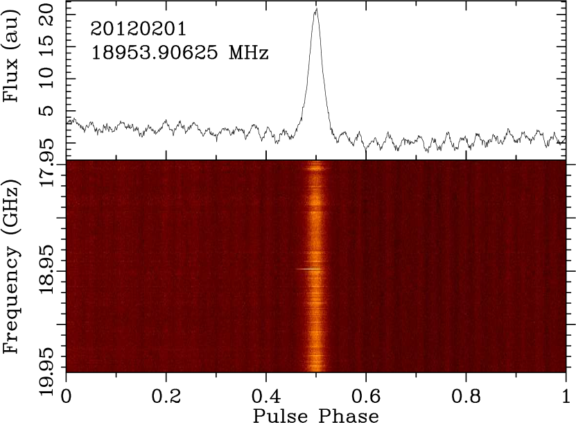
Figure 6: A $10\,{\rm s}$ duration dynamic spectrum centred around the $0.15\,{\rm Jy}$ single pulse event detected at $18.95\,{\rm GHz}$ on February $1^{\rm st}\,2012$. The top panel shows the integrated pulse profile (in arbitrary units) as a function of pulse phase. The lower panel shows frequency subbands, also as a function of pulse phase, across $2\,{\rm GHz}$ around the central observing frequency of $18.95\,{\rm GHz}$. The“ripple-like” instabilities around the main pulse are discussed in Section 3.2.

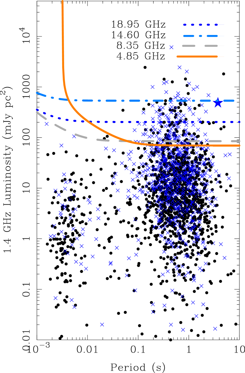
Figure 7: Luminosity at $1.4\,{\rm GHz}$ versus spin period of the known pulsar population (black dots and blue crosses) with luminosity information from the ATNF pulsar catalogue (Manchester et al., 2005). Blue crosses indicate pulsars with a measured spectral index. PSR J1745$-$2900 is indicated by a blue star and its $1.4\,{\rm GHz}$ luminosity was derived using the measured spectral index from multi-frequency observations (Torne et al., 2015). The sensitivity limits of the periodicity searches of our observations of the GC are over plotted with various thick colored lines that are scaled assuming an average pulsar spectral index of $-1.6$, a GC distance of $8.178\,{\rm kpc}$ (Gravity Collaboration et al., 2019) and an average pulse width of $0.05P$. Only luminosity limits for the full observation duration are plotted. The segmentation strategy of the acceleration search decreases sensitivity by a factor of $\sqrt{2}$ upon each consecutive segmentation (thereby raising the lines). Pulse broadening due to scattering follows published measurements (Spitler et al., 2014) and intra-channel dispersion smearing is for a single channel at the central observing frequency assuming a GC DM of $1778\,{\rm cm}^{-3}\,{\rm pc}$, based on observations of PSR J1745$-$2900 (Eatough et al., 2013c).

3.2 A bright transient event at $18.95\,{\rm GHz}$

Single pulse searches of an observation of Sgr A* at $18.95\,{\rm GHz}$ on February $1^{\rm st}\,2012$, revealed a bright ${\rm(S/N\sim 85)}$ broadband single pulse event of duration (or pulse width) $\sim 0.5\,{\rm s}$ on barycentric MJD 55958.3462226 (Figure 6). We estimate a flux density of $0.15\,{\rm Jy}$ with a $6\sigma$ sensitivity of $0.01\,{\rm Jy}$ for pulses of this width. No DM could be measured due to the small sweep across the band at this frequency ($4.4\,{\rm ms}$ across the $2\,{\rm GHz}$ band at a DM equivalent to that of PSR J1745$-$2900 of $1778\,{\rm cm^{-3}}\,{\rm pc}$) and broad pulse profile. Similar individual bright events were also identified in three further Sgr A* observing epochs on barycentric MJDs 55959.2934368, 55968.3290126 and 55988.2245348. Accurate measurements of the relative arrival time of the single pulse events was not possible with the XFFTs backend because it was not connected to the observatory clock. Because of the lack of dispersion smearing as an astrophysical discriminator, we conducted an observation following the same azimuth and elevation track as Sgr A* but at an alternative hour angle. During this observation another single pulse event with similar characteristics was detected on MJD 56030.2241117. This suggested possible source of terrestrial interference, perhaps due to a satellite uplink or downlink which are known to operate in this frequency range. We also note “ripple-like” instabilities around main pulse, possibly suggesting a satellite passing through the primary beam pattern. The possibility of emission from PSR J1745$-$2900 before its first detection on April $28^{\rm th}\,2013$ cannot be ruled out, however such broad individual single pulses have not been observed from this pulsar in subsequent observations (Eatough et al., 2013c; Desvignes et al., 2018).

Table 3: The system temperature, $T_{\rm sys}$, quoted in the various published GC pulsar search analyses. The observing frequency in GHz is indicated in brackets. In all cases both the receiver, GC background and sky temperatures are included in $T_{\rm sys}$. Publications marked with a ${\clubsuit}$ assume a GC background temperature scaled from continuum surveys and those marked with a $*$ performed flux calibration via a noise diode. The $\spadesuit$ symbol denotes that in Deneva et al. (2009) the search was conducted at $2\,{\rm GHz}$, and $T_{\rm sys}$ given at other frequencies was for flux estimates of the discovered pulsars. In Johnston et al. (2006) the system equivalent flux density in units of Jansky has been converted to $T_{\rm sys}$, in units of Kelvin, by use of telescope gain values given in the webpage at the bottom of this table¹¹. Note. errors are not given and frequencies have been rounded to one decimal place for clarity.

Publication	Tel.	$T_{\rm sys}\,({\rm K})$	$T_{\rm sys}\,({\rm K})$	$T_{\rm sys}\,({\rm K})$	"	"	"	"	"	"	"	"
		$1.4\,{\rm GHz}$	$2.0\,{\rm GHz}$	$3.1\,{\rm GHz}$	$4.8\,{\texttt{"}}$	$4.9\,{\texttt{"}}$	$8.4\,{\texttt{"}}$	$9.0\,{\texttt{"}}$	$14.4\,{\texttt{"}}$	$14.6\,{\texttt{"}}$	$14.8\,{\texttt{"}}$	$19.0\,{\texttt{"}}$
Johnston et al. (2006)♣	Pks.	$-$	$-$	$541$	$-$	$-$	$123$	$-$	$-$	$-$	$-$	$-$
Deneva et al. (2009)♣	GBT	$32$	$27\spadesuit$	$-$	$19$	$-$	$-$	$27$	$-$	$-$	$-$	$-$
Macquart et al. (2010)*	GBT	$-$	$-$	$-$	$-$	$-$	$-$	$-$	$35$	$-$	$38$	$-$
This work*	Eff.	$-$	$-$	$-$	$-$	$200$	$126$	$-$	$-$	$194$	$-$	$79$

${}^{11}\;$https://www.parkes.atnf.csiro.au/observing/documentation/users_guide/html/pkug.html#Receiver-Fleet

3.3 Recovered fractions of a Galactic Centre pulsar population

Figure 7 shows the $1.4\,{\rm GHz}$ “pseudo-luminosity” (hereafter termed “luminosity”; given by $L_{1400}=S_{1400}d^{2}$ where $S_{1400}$ is the $1.4\,{\rm GHz}$ flux density and $d$ is the best known distance) of 2125 known pulsars as a function of spin period with information from the ATNF pulsar catalogue version $1.62$ (Manchester et al., 2005). All pulsars in this sample have flux density measurements at either $1.4\,{\rm GHz}$ or $0.4\,{\rm GHz}$ (with the exception of PSR J1745$-$2900, see below). For those pulsars with no flux density information at $1.4\,{\rm GHz}$ ($11\,{\rm per\,cent}$ of the total sample), we extrapolated from $0.4\,{\rm GHz}$ to this frequency using either the known spectral index (pulsars marked with blue crosses have a measured spectral index) or assuming a recently derived average pulsar spectral index of $-1.6$ (Jankowski et al., 2018). For PSR J1745$-$2900 the $1.4\,{\rm GHz}$ flux density was extrapolated from the measurements described in Torne et al. (2015). The $10\sigma$ luminosity sensitivity limits of periodicity search observations presented in this work are marked with various colored and dashed/dotted lines. Each limit is scaled to its value at our chosen “reference frequency” of $1.4\,{\rm GHz}$ also assuming an average pulsar spectral index of $-1.6$ and according to the GC distance. Therefore pulsars that lie above a given limit would be detected with at least $10\sigma$ significance if placed at the GC distance.

The single reference frequency of $1.4\,{\rm GHz}$ is useful for comparing the approximate relative sensitivity of our multi-frequency search observations and for determining what fraction of a hypothetical GC pulsar population could be detected (Cordes et al., 2004). For instance, assuming the GC pulsar population follows the same luminosity distribution as the currently known pulsars, have an intrinsic pulse width of $0.05P$ and neglecting any binary motion, we determine that approximately 11, 10, one and four per cent of this pulsar population would be detected at $4.85,\,8.35,\,14.6,\,{\rm and}\,18.95\,{\rm GHz}$ respectively. Assuming a larger intrinsic pulse width of $0.1P$ the detected percentages are reduced marginally to eight, seven, one and three per cent at $4.85,\,8.35,\,14.6,\,{\rm and}\,18.95\,{\rm GHz}$ respectively.

Differences in the recovered population fraction can occur when scaling pulsar flux densities to alternative reference frequencies (particularly at the two highest frequencies of $14.6$ and $18.95\,{\rm GHz}$). Because our observations cover a wide range in observing frequency, we have created and analysed the equivalent period luminosity diagrams at each frequency independently. In these analyses frequency scaling of the survey luminosity limits is not required. Also, to address the physical property of the observed spread in pulsar spectral indices, we have investigated the effects of choosing not just a single average spectral index (for those pulsars with no spectral index information) but a random selection from a Gaussian distribution with an average spectral index of $-1.6$ and a standard deviation of $0.54$, as given in Jankowski et al. (2018). These results (and those at the reference frequency of $1.4\,{\rm GHz}$) are presented in Appendix A in Table 4 and can be seen in Figures 10 and 11. The effects of possible broken spectral power laws have not been taken into account and the numbers reported should be treated as approximate upper limits. We note that despite accounting for both effects described above, in all cases the recovered fraction of pulsars from this hypothetical population is no better than 13 per cent, illustrating that the intrinsic sensitivity of these observations to typical pulsars at the GC is still markedly low. The reductions in $T_{\rm obs}$ applied in our acceleration search for compact binary systems compound this sensitivity problem further. Similar population detection analyses have recently been given in the results from GC pulsar searches conducted at millimetre wavelengths (Torne et al., 2021; Liu et al., 2021).

In addition, Lazarus et al. (2015) have shown that the sensitivity of pulsar searches in the Arecibo pulsar ALFA (PALFA) survey at $1.4\,{\rm GHz}$ degrades (by up to a factor of 10) for spin periods above $100\,{\rm ms}$ due to red noise and RFI effects present in their data. To investigate if such effects are observed in the data used in this work $-$ where in particular atmospheric fluctuations may produce red noise features $-$ we have injected simulated pulsar signals into example data sets at each observing frequency and measured any reductions in sensitivity. Evidence for a radio frequency dependence in the detrimental effects on sensitivity has been found, which we would indeed expect for red noise dominated by atmospheric effects which worsen towards K-band (see Figure 12). This analysis is described in detail in Appendix B along with the updated sensitivity, accounting for red noise effects for spin periods $>0.1\,{\rm s}$, plotted in Figures 10 and 11. The recovered fraction of pulsars are further reduced by a few percentage points due to these effects and is indicated in Table 4 by the numbers in parentheses.

4 Discussion

During the course of this work a number of aspects regarding the efficacy of searches for pulsars in the GC have been identified. In the following subsections we discuss two more areas of importance and finish by looking at some of the future prospects for GC pulsar searches.

4.1 Background sky brightness temperature toward the GC

As noted in Johnston et al. (2006) and Macquart et al. (2010), and as shown in Table 2, the GC background brightness temperature, $T_{\rm GC}$, can have a significant effect on the sensitivity of GC pulsar searches. In Table 3 the various measurements, or estimates, of $T_{\rm sys}$ whilst on source (therefore including $T_{\rm GC}$) in published GC pulsar searches have been collected and placed with the calibrated measurements from this work. There is a large discrepancy between the figures presented in observations performed at the lowest frequencies $\nu<3.1\,{\rm GHz}$ in Johnston et al. (2006) and Deneva et al. (2009). From our measurements outlined in Table 2, and the discussion in Johnston et al. (2006), we expect $T_{\rm GC}$ to dominate $T_{\rm sys}$ for frequencies $\lesssim 8\,{\rm GHz}$. For example we already find $T_{\rm GC}=137(16)\,{\rm K}$ at the frequency of $4.85\,{\rm GHz}$ $-$ in tension with the estimates of $T_{\rm sys}$ of $19\,{\rm K}$ at $4.8\,{\rm GHz}$ in Deneva et al. (2009). At higher frequencies of $8.4\,{\rm GHz}$ our measurements are consistent with those estimates presented in Johnston et al. (2006). At frequency $14.6\,{\rm GHz}$ our measurement appears to be in conflict with that given at $14.8\,{\rm GHz}$ in Macquart et al. (2010). We postulate that the sensitivity at Effelsberg might have been degraded due to both the extremely low elevation of Sgr A* (although measurements of $T_{\rm sys}$ at $14.6\,{\rm GHz}$ in the Sgr A* ON and Sgr A* OFF positions suggest this is not the case $-$ see Table 2), poor atmospheric conditions during the single calibration observation at this frequency and the higher receiver temperature. Repeated measurements at this frequency would have been beneficial in resolving this discrepancy.

The addition of our measurements to existing published figures highlights some inconsistencies and also an overall sparsity of directly calibrated sensitivity measurements in GC pulsar searches. While continuum measurements of the GC region with single dish telescopes (e.g. Reich et al. 1990; Law et al. 2008) have been beneficial for estimating the sensitivity of pulsar searches, these cannot take into account weather or instrumental effects during the pulsar search.

4.2 Binary search considerations for pulsars closely orbiting Sgr A*

For searches of orbiting pulsars, Sgr A* presents a unique set of conditions because of its extreme mass. Even pulsars in long period orbits $(P_{\rm b}\lesssim 800\,{\rm d})$ can undergo sufficiently large acceleration that the methods used in this work which search for signals with constant spin frequency drift in the Fourier spectrum (viz. presto accelsearch) can be overcome. In Figure 8 we plot the number of spectral bins drifted in the Fourier spectrum as a function of orbital period around Sgr A* for pulsars in circular orbits, for a number of representative spin periods and observation lengths (Figure 8 panels a, b and c). The intersection of diagonal lines with the horizontal dot dashed line (the current maximum value of $n_{\rm drift}$ searched given by the zmax parameter in accelsearch) gives the lower limit of the orbital period for a pulsar with fundamental, or harmonics, of that spin frequency that are detectable. Because $n_{\rm drift}\propto T_{\rm obs}^{2}$, the smearing of spectral features is much larger in the necessarily deep observations that might be required to detect pulsars at the GC distance ($T_{\rm obs}=6-9\,{\rm h}$, for $100\,{\rm m}$ class dishes). For example, if a maximum spin frequency of $1000\,{\rm Hz}$ is considered (a spin frequency that covers known MSPs and most of their harmonics) the minimum circular orbital periods around Sgr A* detectable are: $P_{\rm b}\sim 780\,{\rm d}$, $a=0.3\,{\rm m\,s^{-2}}$ for $T_{\rm obs}=9\,{\rm h}$; $P_{\rm b}\sim 420\,{\rm d}$, $a=0.8\,{\rm m\,s^{-2}}$ for $T_{\rm obs}=6\,{\rm h}$ and $P_{\rm b}\sim 150\,{\rm d}$, $a=3.1\,{\rm m\,s^{-2}}$ for $T_{\rm obs}=3\,{\rm h}$. For longer spin periods the minimum orbital periods detectable are correspondingly shorter.

For the purpose of investigating how robust binary pulsar searches around Sgr A* are, a useful physical minimum orbital period to consider can be inferred by setting the time scale of coalescence due to the emission of gravitational waves, $\tau_{\rm GW}$, equal to the typical lifetime of a pulsar, $\tau_{\rm PSR},$ where $\tau_{\rm PSR}\sim 10^{7}\,{\rm y}$ (P. Freire private comm. and see Appendix A2.7 in Lorimer & Kramer 2012). Such an exercise results in $P_{\rm b}\simeq 50\,{\rm h}$, average velocity $0.09\,c$ and a maximum l.o.s acceleration of $\simeq 1000\,{\rm m\,s^{-2}}$ for systems viewed edge-on. Orbital accelerations of similar magnitude are currently only seen in extremely compact or compact and eccentric binary double neutron star (DNS) systems such as e.g. PSR J0737$-$3039A/B and PSR J1757$-$1854 (Kramer et al., 2006b; Cameron et al., 2018). The comparatively longer orbital period of the hypothetical Sgr A* pulsar described above means that higher order effects detrimental to binary pulsar searches $-$ such as the rate of change of acceleration, known as “jerk” $-$ are reduced. This effect is illustrated explicitly in Figure 9 where the acceleration and jerk of a pulsar throughout one orbit of a hypothetical compact $(P_{\rm b}=2.4\,{\rm h})$ pulsar stellar mass black hole, NS$-$SBH, and an extreme $(P_{\rm b}=50.0\,{\rm h})$ NS$-$Sgr A* system are plotted. The acceleration in both systems is approximately equivalent, peaking at around $1000\,{\rm m}\,{\rm s}^{-2}$ whereas the jerk exhibited by the NS$-$Sgr A* is roughly 20 times smaller than that of the NS$-$SBH. Using the commonly accepted limit for the application of acceleration searches that $T_{\rm obs}<P_{\rm b}/10$ (Ransom et al., 2003; Ng et al., 2015), higher order jerk effects in the Sgr A* pulsars described above should only become relevant for observations where $T_{\rm obs}\gtrsim 5\,{\rm h}$ for the the most extreme $P_{b}=50\,{\rm h}$ system.

Potential expansion of the zmax term in presto accelsearch specifically to deal with the demands of deep acceleration searches of the Sgr A* region are currently under discussion (S. Ransom private comm.). We also note that the most recent versions of presto accelsearch can now search for and compensate higher order quadratic frequency drifts due to jerk (Andersen & Ransom, 2018), potentially increasing the integration time that can be searched for binaries. For extremely long observations $(T_{\rm obs}\sim 9\,{\rm h})$ time domain orbital template matching techniques will likely offer the highest sensitivity to a wide range of GC binary pulsars (Knispel et al., 2013; Allen et al., 2013).

Figure 8: The theoretical number of spectral bins the spin frequency $f$ (or period $P$) drifts in the Fourier spectrum for pulsars in circular orbits around Sgr A*, for three representative observation lengths of $3$, $6$ and $9\,{\rm h}$ (panels a, b and c respectively) and which occur at the phase of the orbit where the l.o.s. acceleration is at a maximum. For the orbital period and observation length ranges plotted, the l.o.s. acceleration can be assumed to be approximately constant. The dot dashed horizontal line indicates the $z_{\rm max}$ value used in this work of 1200 and the vertical dashed line shows the orbital period for a pulsar in an orbit with a merger time of $10^{7}\,{\rm y}$ $-$ the typical lifetime of a normal pulsar.

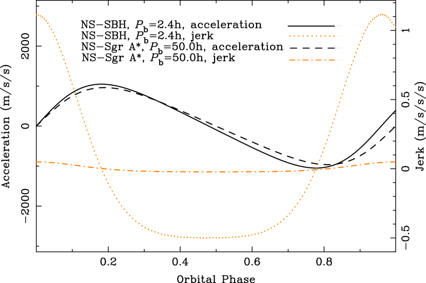
Figure 9: l.o.s acceleration and jerk as a function of orbital phase for two extreme pulsar black hole systems viewed edge on to the orbital plane. The solid black and orange dotted lines represent the acceleration and jerk (respectively) in a compact pulsar stellar mass black hole binary (NS$-$SBH, $P_{\rm b}\,=\,2.4\,{\rm h}$, $e=0.1,m_{\rm c}=30\,{\rm M_{\odot}}$). The dashed black and dot-dashed orange lines mark the acceleration and jerk of a pulsar closely orbiting Sgr A* (NS$-$Sgr A*, $P_{\rm b}=50.0\,{\rm h}$, $e=0.1$, $m_{\rm c}=4\times 10^{6}\,{\rm M_{\odot}}$).

4.3 Prospects for future pulsar searches of the GC

The conditions in and toward the GC create a “perfect storm” of observational requirements that are detrimental to searches for radio pulsars. In no particular order these are: its large distance ($\sim 84\,{\rm per\,cent}$ of known pulsars are closer than the GC due to their relative weakness as radio sources - Liu & Eatough, 2017); high levels of pulse scattering (while scattering might be less than previously predicted it is still large enough to smear out MSPs at frequencies $\lesssim 7\,{\rm GHz}$ - Spitler et al., 2014); intense background emission (the GC is the brightest region of the Galaxy at radio wavelengths reducing system sensitivity - Section 2.3); the typically steep spectrum of pulsar emission (at the high frequencies necessary to combat scattering pulsar emission is weaker); long observation times (the combined effects of steep pulsar spectra and the large GC distance currently necessitate long observations that can reduce sensitivity to binary pulsars or pulsars orbiting Sgr A* - Section 4.2).

To combat all of these effects simultaneously an interferometer with large collecting area and that operates at frequencies $\gtrsim 7\,{\rm GHz}$ is optimal. Interferometers offer the added benefit of resolving out part of the bright GC background that single dishes are exposed to. The relative weight of each of these effects and the optimal balance of observing parameters is not yet fully understood, however, pulsar searches using interferometers are already underway with Atacama Large Millimeter/submillimeter Array (ALMA) (Liu et al., 2021) and the Karl G. Jansky Very Large Array (VLA) (Wharton, 2017). To fully rule out scattering effects in the GC, multi-epoch searches for flat spectrum pulsars have been conducted at millimetre wavelengths with the Institut de Radioastronomie Millimétrique (IRAM) $30\,{\rm m}$ telescope (Torne et al., 2021). At Effelsberg, GC pulsar searches with nearly three times the sensitivity of those presented here (thanks to a new a broad-band $4-8\,{\rm GHz}$ receiver) will be given by Desvignes et al. (in prep.).

The instantaneous sensitivity for pulsar searches offered by next generation telescopes such as MeerKat (Stappers & Kramer, 2016; Kramer et al., 2016), Next Generation VLA (ngVLA - Bower et al., 2019) and SKA1-mid (Eatough et al., 2015) might allow at least an order of magnitude improvement in survey depth and will also facilitate an increased binary parameter space that can be searched thanks to the reduction in the necessary integration length.

5 Summary

A multi-epoch survey for binary pulsars and fast transients in the Galactic Centre at frequencies $(4.85,\,8.35,\,14.60,\,18.95)\,{\rm GHz}$ was carried out between February 2012 and February 2016 using the Effelsberg 100-m radio telescope. The various high radio frequencies utilized decrease the deleterious effects of strong pulse scattering that exist in this region. Comprehensive acceleration searches have been conducted on progressively shorter segments of the full observation lengths to increase sensitivity to relativistic binary pulsars. This survey is the first time that observations of the Galactic Centre have been regularly repeated over a time-span of the order of years; highly beneficial for detecting pulsars undergoing relativistic binary motion or exhibiting transient phenomena. An anomalous repeating signal with a spin period close to that of PSR J1745$-$2900 and a handful of single pulse events have been identified, but no previously unknown pulsars have been detected. Sensitivity measurements of our observing system have revealed that, at best, only 13 per cent of the known pulsar population could be detected by these searches if it were placed at the Galactic Centre distance. We also show that analysis of current or future deep observations $(9\,{\rm h})$ with existing pulsar search tools may struggle to detect some millisecond pulsars in orbits of less than $800\,{\rm d}$ around Sgr A*. Through accurate calibration of our observing system and investigation into previously unaccounted effects we demonstrate that earlier pulsar searches of the Galactic Centre may have overestimated their sensitivity. Future observatories with increased sensitivity, and the use of interferometers in periodicity searches, will improve the power to discover as yet undetected Galactic Centre pulsars.

DATA AVAILABILITY

The data underlying this article will be shared on reasonable request to the corresponding author.

Appendix A Alternative period luminosity diagrams

In this section we outline the recovered fractions of a hypothetical GC pulsar population after scaling the known pulsar population flux densities (and corresponding luminosity) to each individual observing frequency presented in this work. At each reference frequency we have used both the known spectral index and either a simple average spectral index of $-1.6$ or a random selection from a Gaussian distribution of spectral indices with mean $-1.6$ and standard deviation of $0.54$ (to model the observed spread in pulsar spectral indices) as given in Jankowski et al. (2018). The different frequency scaling types are listed in Table 4. At $1.4\,{\rm GHz}$ the majority of pulsars have a known flux density and are therefore not frequency scaled. The effects of these alternative analyses changes the recovered fractions by just one to three percentage points at $4.85$ and $8.35\,{\rm GHz}$. At our highest observing frequencies of $14.6$ and $18.95\,{\rm GHz}$, the recovered fractions of a population can increase by just over a factor of two compared to the same analysis with a reference frequency of $1.4\,{\rm GHz}$. For high frequency pulsar searches we therefore suggest these analyses should be performed at the observing frequency being used (see e.g. Torne et al. 2021; Liu et al. 2021), however for most pulsars it is still not known if spectral indices are constant over wide frequency ranges (see e.g. Kramer et al., 1996b). The alternative period luminosity diagrams corresponding to the analyses are presented in Figures 10 and 11. These figures also contain luminosity limits that account for measured red noise effects (red lines) above spin periods of $0.1\,{\rm s}$ - see Appendix B for details. Because of such effects, the recovered fractions of GC pulsars given here should be treated as approximate upper limits.

Table 4: The estimated recovered fractions of a hypothetical GC pulsar population by the searches conducted in this work (and displayed in Figures 7, 10 and 11). $2125$ pulsars with flux density measurements at either $1.4\,{\rm GHz}$ or $0.4\,{\rm GHz}$, known or unknown spectral indices and distance estimates from version 1.62 of the ATNF pulsar catalogue form the sample. Each column can be summarised as follows: “Ref. frequency” indicates the reference frequency at which the luminosity is given and plotted; “PSR scaling index type” is how the luminosity of pulsars, with both known and unknown spectral indices, are scaled to the reference frequency (see table footnote for further details and we note that no scaling was required at $1.4\,{\rm GHz}$ for pulsars with known $S_{\rm 1400}$); “Pulse width” gives the assumed pulse width as a fraction of the pulse period. At 1.4 GHz all luminosity limits are frequency scaled assuming an average pulsar spectral index of $-1.6$ as given in Jankowski et al. (2018). In all cases a single power law function is assumed. Numbers in parentheses account for the reduction in sensitivity caused by red noise effects described in Appendix B.

Ref. frequency	PSR scaling	Pulse	$4.85\,{\rm GHz}$	$8.35\,{\rm GHz}$	$14.6\,{\rm GHz}$	$18.95\,{\rm GHz}$	Associated
	index type	width					figure
$1.4\,{\rm GHz}$	(a)	$0.05P$	$11\%$	$10\%$	$1\%$	$4\%$	Fig. 7
$1.4\,{\rm GHz}$	(a)	$0.10P$	$8\%$	$7\%$	$1\%$	$3\%$	$-$
$1.4\,{\rm GHz}$	(b)	$0.05P$	$12\%$	$10\%$	$1\%$	$4\%$	$-$
$1.4\,{\rm GHz}$	(b)	$0.10P$	$8\%$	$7\%$	$1\%$	$3\%$	$-$
$4.85\,{\rm GHz}$	(c)	$0.05P$	$12(9)\%$	$-$	$-$	$-$	Fig. 10
$4.85\,{\rm GHz}$	(c)	$0.10P$	$9\%$	$-$	$-$	$-$	$-$
$4.85\,{\rm GHz}$	(d)	$0.05P$	$13\%$	$-$	$-$	$-$	$-$
$4.85\,{\rm GHz}$	(d)	$0.10P$	$10\%$	$-$	$-$	$-$	$-$
$8.35\,{\rm GHz}$	(c)	$0.05P$	$-$	$11(8)\%$	$-$	$-$	Fig. 10
$8.35\,{\rm GHz}$	(c)	$0.10P$	$-$	$8\%$	$-$	$-$	$-$
$8.35\,{\rm GHz}$	(d)	$0.05P$	$-$	$13\%$	$-$	$-$	$-$
$8.35\,{\rm GHz}$	(d)	$0.10P$	$-$	$10\%$	$-$	$-$	$-$
$14.6\,{\rm GHz}$	(c)	$0.05P$	$-$	$-$	$3(1)\%$	$-$	Fig. 11
$14.6\,{\rm GHz}$	(c)	$0.10P$	$-$	$-$	$2\%$	$-$	$-$
$14.6\,{\rm GHz}$	(d)	$0.05P$	$-$	$-$	$4\%$	$-$	$-$
$14.6\,{\rm GHz}$	(d)	$0.10P$	$-$	$-$	$3\%$	$-$	$-$
$18.95\,{\rm GHz}$	(c)	$0.05P$	$-$	$-$	$-$	$6(4)\%$	Fig. 11
$18.95\,{\rm GHz}$	(c)	$0.10P$	$-$	$-$	$-$	$5\%$	$-$
$18.95\,{\rm GHz}$	(d)	$0.05P$	$-$	$-$	$-$	$9\%$	$-$
$18.95\,{\rm GHz}$	(d)	$0.10P$	$-$	$-$	$-$	$6\%$	$-$

PSR scaling index types: (a) none and $-1.6$; (b) none and rand.; (c) known and $-1.6$; (d) known and rand.

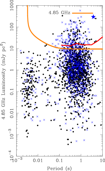
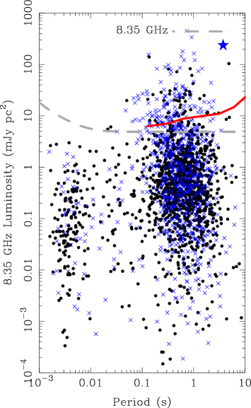
Figure 10: Luminosity versus spin period of the known pulsar population at $4.85\,{\rm GHz}$ (left hand panel) and $8.35\,{\rm GHz}$ (right hand panel). In these diagrams the pulsar luminosity is scaled from either $1.4\,{\rm GHz}$ and $0.4\,{\rm GHz}$ using the known spectral index (pulsars with an index are marked with blue crosses) or a spectra index of $-1.6$. The estimate of the $10\sigma$ sensitivity limit of our GC search observation (for the maximum observing duration) is marked with a line. The red line indicates measured $10\sigma$ sensitivity limits from the injection of simulated pulsar signals which account for red noise effects. See Appendix B for more details about this limit.

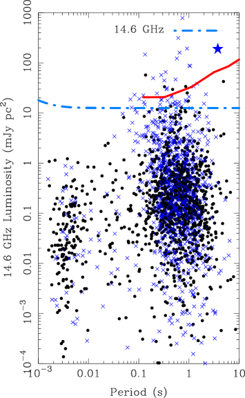
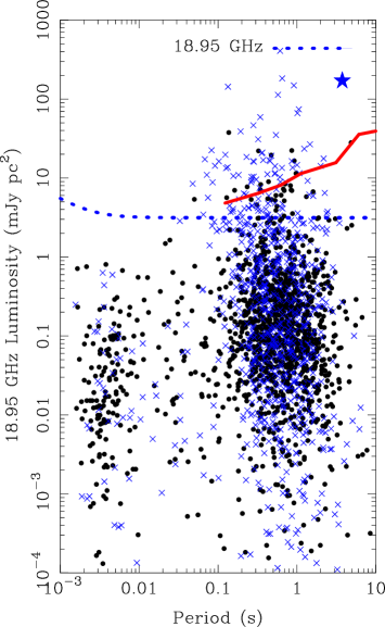
Figure 11: Luminosity versus spin period of the known pulsar population at $14.6\,{\rm GHz}$ (left hand panel) and $18.95\,{\rm GHz}$ (right hand panel). In these diagrams the pulsar luminosity is scaled from either $1.4\,{\rm GHz}$ and $0.4\,{\rm GHz}$ using the known spectral index (pulsars with an index are marked with blue crosses) or a spectra index of $-1.6$. The estimate of the $10\sigma$ sensitivity limit of our GC search observation (for the maximum observing duration) is marked with a line. The red line indicates measured $10\sigma$ sensitivity limits from the injection of simulated pulsar signals which account for red noise effects. See Appendix B for more details about this limit.

Appendix B The effects of low fluctuation frequency noise on sensitivity

It has been shown that a combination of RFI and low frequency (viz. fluctuation frequency) noise variations (red noise) in the $1.4\,{\rm GHz}$ radio observing system of the Arecibo Pulsar ALFA (PALFA) survey, adversely impacts the sensitivity to longer period ($P\gtrsim 0.1\,{\rm s}$) pulsars (Lazarus et al., 2015). At the observing frequencies presented in this work, we detect considerably less RFI than Effelsberg observations at $1.4\,{\rm GHz}$, however RFI is still present and red noise effects might occur due to atmospheric opacity variations and/or receiver/backend fluctuations. To examine these effects we have performed the following tests:

Simulated pulsar signals have been injected into examples of both the real observational data and simulated data consisting of purely Gaussian white noise. The latter forms our “baseline” from which we can measure sensitivity losses empirically. We have made use of the presto routine makedata to simulate both noise free pulsar signals and time series of purely Gaussian white noise. Firstly we take an example dedispersed time series (dedispersed to the DM of PSR J1745$-$2900 of $1778\,{\rm cm}^{-3}\,{\rm pc}$) at a given frequency of either $4.85,\,8.35,\,14.60$ or $18.95\,{\rm GHz}$. The “DC offset” of this time series (effectively the value of $T_{\rm sys}$ in un-calibrated machine counts) is then measured in order to simulate a time series with equivalent standard deviation fluctuations (assuming Poisson statistics) after running the procedure of red noise removal with the presto routine rednoise, as is done in our pipeline (Section 2.2). The noise free pulsar signal of a period $P$ and width $0.05P$ is then injected into the simulated white noise data where the spectral detection $\sigma$ value is measured with accelsearch. The same simulated noise free pulsar signal is then injected into the real survey data after which red nose removal is performed and the spectral detection $\sigma$ is also measured with accelsearch. We then find the relative reduction factor in spectral $\sigma$ as a function of spin period. Non-integer spin periods of $0.123,\,0.323,\,...\,10.123\,{\rm s}$ have been simulated in order to minimise coincidences with terrestrial RFI signals (which often occur around integer spin periods) that could bias results. The reduction factor in accelsearch spectral $\sigma$ is plotted for each frequency in Figure 12. Note the apparent worsening of effects with increasing observing frequency. This might be caused by the increased effects of atmospheric opacity variations at higher frequencies.

The reduction factor in spectral $\sigma$ allows us to scale the $10\sigma$ luminosity survey limits as a function of spin period and is plotted with red lines in Figures 10 and 11. The effects on the recovered fraction of a GC pulsar population are also indicated in Table 4 by the numbers given in parentheses. Recovered fractions are reduced by a few percentage points at all frequencies with proportionately the biggest effects at at $14.6$ and $18.95\,{\rm GHz}$. Further in depth multi-epoch analyses are required to fully account for changing atmospheric conditions.

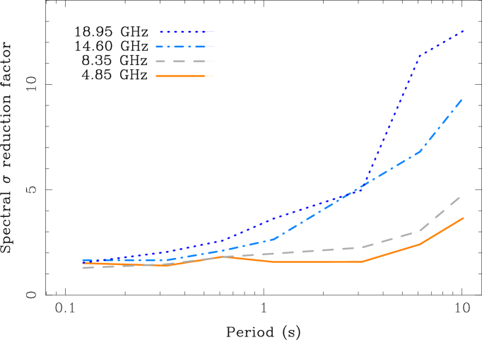
Figure 12: The measured reduction factor of spectral $\sigma$ given in accelsearch due to red noise effects as a function of spin period. See Appendix B for details of how the reduction factor was measured.

References

- Allen et al. (2013) Allen B., et al., 2013, ApJ, 773, 91
- Andersen & Ransom (2018) Andersen B. C., Ransom S. M., 2018, ApJ, 863, L13
- Bower et al. (2014) Bower G. C., et al., 2014, ApJ, 780, L2
- Bower et al. (2019) Bower G., et al., 2019, BAAS, 51, 438
- Breton et al. (2008) Breton R. P., et al., 2008, Science, 321, 104
- Cameron et al. (2018) Cameron A. D., et al., 2018, MNRAS, 475, L57
- Chennamangalam & Lorimer (2014) Chennamangalam J., Lorimer D. R., 2014, MNRAS, 440, L86
- Cordes & Lazio (1997a) Cordes J. M., Lazio T. J. W., 1997a, ApJ, 475, 557
- Cordes & Lazio (1997b) Cordes J. M., Lazio T. J. W., 1997b, ApJ, 475, 557
- Cordes & Lazio (2002) Cordes J. M., Lazio T. J. W., 2002, arXiv e-prints, pp astro–ph/0207156
- Cordes et al. (2004) Cordes J. M., Kramer M., Lazio T. J. W., Stappers B. W., Backer D. C., Johnston S., 2004, New A Rev., 48, 1413
- Deneva (2010) Deneva J. S., 2010, PhD thesis, Cornell University
- Deneva et al. (2009) Deneva J. S., Cordes J. M., Lazio T. J. W., 2009, ApJ, 702, L177
- Desvignes et al. (2018) Desvignes G., et al., 2018, ApJ, 852, L12
- Desvignes et al. (2019) Desvignes G., et al., 2019, Science, 365, 1013
- Dexter et al. (2017) Dexter J., et al., 2017, MNRAS, 471, 3563
- Dimoudi et al. (2018) Dimoudi S., Adamek K., Thiagaraj P., Ransom S. M., Karastergiou A., Armour W., 2018, The Astrophysical Journal Supplement Series, 239, 28
- Do et al. (2019) Do T., et al., 2019, Science
- Eatough et al. (2013a) Eatough R. P., Kramer M., Klein B., Karuppusamy R., Champion D. J., Freire P. C. C., Wex N., Liu K., 2013a, in van Leeuwen J., ed., IAU Symposium Vol. 291, IAU Symposium. pp 382–384 (arXiv:1210.3770), doi:10.1017/S1743921312024209
- Eatough et al. (2013b) Eatough R. P., Kramer M., Lyne A. G., Keith M. J., 2013b, MNRAS, 431, 292
- Eatough et al. (2013c) Eatough R. P., et al., 2013c, Nature, 501, 391
- Eatough et al. (2015) Eatough R., et al., 2015, Advancing Astrophysics with the Square Kilometre Array (AASKA14), p. 45
- Eckart & Genzel (1996) Eckart A., Genzel R., 1996, Nature, 383, 415
- Event Horizon Telescope Collaboration et al. (2019) Event Horizon Telescope Collaboration et al., 2019, ApJ, 875, L1
- Faucher-Giguère & Loeb (2011) Faucher-Giguère C.-A., Loeb A., 2011, MNRAS, 415, 3951
- Faulkner et al. (2004) Faulkner A. J., et al., 2004, MNRAS, 355, 147
- Freire (2005) Freire P. C. C., 2005, in Rasio F. A., Stairs I. H., eds, Astronomical Society of the Pacific Conference Series Vol. 328, Binary Radio Pulsars. p. 405 (arXiv:astro-ph/0404105)
- Genzel et al. (2010) Genzel R., Eisenhauer F., Gillessen S., 2010, Reviews of Modern Physics, 82, 3121
- Ghez et al. (2003) Ghez A. M., et al., 2003, ApJ, 586, L127
- Ghez et al. (2008) Ghez A. M., et al., 2008, ApJ, 689, 1044
- Gillessen et al. (2009) Gillessen S., Eisenhauer F., Trippe S., Alexander T., Genzel R., Martins F., Ott T., 2009, ApJ, 692, 1075
- Gravity Collaboration et al. (2018) Gravity Collaboration et al., 2018, A&A, 615, L15
- Gravity Collaboration et al. (2019) Gravity Collaboration et al., 2019, A&A, 625, L10
- Jankowski et al. (2018) Jankowski F., van Straten W., Keane E. F., Bailes M., Barr E. D., Johnston S., Kerr M., 2018, MNRAS, 473, 4436
- Jessner et al. (2005) Jessner A., Słowikowska A., Klein B., Lesch H., Jaroschek C. H., Kanbach G., Hankins T. H., 2005, Advances in Space Research, 35, 1166
- Johnston et al. (1992) Johnston S., Manchester R. N., Lyne A. G., Bailes M., Kaspi V. M., Qiao G., D’Amico N., 1992, ApJ, 387, L37
- Johnston et al. (2006) Johnston S., Kramer M., Lorimer D. R., Lyne A. G., McLaughlin M., Klein B., Manchester R. N., 2006, MNRAS, 373, L6
- Karako-Argaman et al. (2015) Karako-Argaman C., et al., 2015, ApJ, 809, 67
- Keith et al. (2009) Keith M. J., Eatough R. P., Lyne A. G., Kramer M., Possenti A., Camilo F., Manchester R. N., 2009, MNRAS, 395, 837
- Klein (2005) Klein B., 2005, PhD thesis, Rheinischen Friedrich-Wilhelms-Universität Bonn
- Klein et al. (2004) Klein B., Kramer M., Müller P., Wielebinski R., 2004, in Camilo F., Gaensler B. M., eds, Vol. 218, Young Neutron Stars and Their Environments. p. 133
- Knispel et al. (2013) Knispel B., et al., 2013, ApJ, 774, 93
- Kramer (1998) Kramer M., 1998, ApJ, 509, 856
- Kramer et al. (1996a) Kramer M., Jessner A., Muller P., Wielebinski R., 1996a, in Johnston S., Walker M. A., Bailes M., eds, Astronomical Society of the Pacific Conference Series Vol. 105, IAU Colloq. 160: Pulsars: Problems and Progress. p. 13
- Kramer et al. (1996b) Kramer M., Xilouris K. M., Jessner A., Wielebinski R., Timofeev M., 1996b, A&A, 306, 867
- Kramer et al. (2000) Kramer M., Klein B., Lorimer D., Müller P., Jessner A., Wielebinski R., 2000, in Kramer M., Wex N., Wielebinski R., eds, Astronomical Society of the Pacific Conference Series Vol. 202, IAU Colloq. 177: Pulsar Astronomy - 2000 and Beyond. p. 37 (arXiv:astro-ph/0002117)
- Kramer et al. (2004) Kramer M., Backer D. C., Cordes J. M., Lazio T. J. W., Stappers B. W., Johnston S., 2004, New A Rev., 48, 993
- Kramer et al. (2006a) Kramer M., Lyne A. G., O’Brien J. T., Jordan C. A., Lorimer D. R., 2006a, Science, 312, 549
- Kramer et al. (2006b) Kramer M., et al., 2006b, Science, 314, 97
- Kramer et al. (2016) Kramer M., et al., 2016, in MeerKAT Science: On the Pathway to the SKA. p. 3
- Law et al. (2008) Law C. J., Yusef-Zadeh F., Cotton W. D., Maddalena R. J., 2008, The Astrophysical Journal Supplement Series, 177, 255
- Lazarus et al. (2015) Lazarus P., et al., 2015, ApJ, 812, 81
- Lazarus et al. (2016) Lazarus P., Karuppusamy R., Graikou E., Caballero R. N., Champion D. J., Lee K. J., Verbiest J. P. W., Kramer M., 2016, MNRAS, 458, 868
- Lazio & Cordes (1998a) Lazio T. J. W., Cordes J. M., 1998a, ApJS, 118, 201
- Lazio & Cordes (1998b) Lazio T. J. W., Cordes J. M., 1998b, ApJ, 505, 715
- Lee et al. (2013) Lee K. J., et al., 2013, MNRAS, 433, 688
- Liu & Eatough (2017) Liu K., Eatough R., 2017, Nature Astronomy, 1, 812
- Liu et al. (2012) Liu K., Wex N., Kramer M., Cordes J. M., Lazio T. J. W., 2012, ApJ, 747, 1
- Liu et al. (2021) Liu K., et al., 2021, arXiv e-prints, p. arXiv:2104.08986
- Lorimer & Kramer (2012) Lorimer D. R., Kramer M., 2012, Handbook of Pulsar Astronomy. Cambridge University Press
- Macquart & Kanekar (2015) Macquart J. P., Kanekar N., 2015, ApJ, 805, 172
- Macquart et al. (2010) Macquart J. P., Kanekar N., Frail D. A., Ransom S. M., 2010, ApJ, 715, 939
- Manchester et al. (2005) Manchester R. N., Hobbs G. B., Teoh A., Hobbs M., 2005, AJ, 129, 1993
- Muno et al. (2005) Muno M. P., Pfahl E., Baganoff F. K., Brandt W. N., Ghez A., Lu J., Morris M. R., 2005, ApJ, 622, L113
- Ng et al. (2015) Ng C., et al., 2015, MNRAS, 450, 2922
- Paumard et al. (2001) Paumard T., Maillard J. P., Morris M., Rigaut F., 2001, A&A, 366, 466
- Pedlar et al. (1989) Pedlar A., Anantharamaiah K. R., Ekers R. D., Goss W. M., van Gorkom J. H., Schwarz U. J., Zhao J.-H., 1989, ApJ, 342, 769
- Psaltis et al. (2016) Psaltis D., Wex N., Kramer M., 2016, ApJ, 818, 121
- Rajwade et al. (2017) Rajwade K. M., Lorimer D. R., Anderson L. D., 2017, MNRAS, 471, 730
- Ransom (2001) Ransom S. M., 2001, PhD thesis, Harvard University
- Ransom et al. (2002) Ransom S. M., Eikenberry S. S., Middleditch J., 2002, AJ, 124, 1788
- Ransom et al. (2003) Ransom S. M., Cordes J. M., Eikenberry S. S., 2003, ApJ, 589, 911
- Rea et al. (2013) Rea N., et al., 2013, The Astronomer’s Telegram, 5032, 1
- Reich et al. (1990) Reich W., Fuerst E., Reich P., Reif K., 1990, A&AS, 85, 633
- Reid & Brunthaler (2004) Reid M. J., Brunthaler A., 2004, ApJ, 616, 872
- Roy et al. (2004) Roy A. L., Teuber U., Keller R., 2004, in European VLBI Network on New Developments in VLBI Science and Technology. pp 265–270
- Schnitzeler et al. (2016) Schnitzeler D. H. F. M., Eatough R. P., Ferrière K., Kramer M., Lee K. J., Noutsos A., Shannon R. M., 2016, MNRAS, 459, 3005
- Shannon & Johnston (2013) Shannon R. M., Johnston S., 2013, MNRAS, 435, L29
- Siemion et al. (2013) Siemion A., et al., 2013, in van Leeuwen J., ed., Vol. 291, Neutron Stars and Pulsars: Challenges and Opportunities after 80 years. pp 57–57, doi:10.1017/S1743921312023149
- Spitler et al. (2014) Spitler L. G., et al., 2014, ApJ, 780, L3
- Stappers & Kramer (2016) Stappers B., Kramer M., 2016, in MeerKAT Science: On the Pathway to the SKA. p. 9
- Torne et al. (2015) Torne P., et al., 2015, MNRAS, 451, L50
- Torne et al. (2021) Torne P., et al., 2021, A&A, 650, A95
- Wang et al. (2006) Wang Q. D., Lu F. J., Gotthelf E. V., 2006, MNRAS, 367, 937
- Wex (2014) Wex N., 2014, arXiv e-prints, p. arXiv:1402.5594
- Wex & Kopeikin (1999) Wex N., Kopeikin S. M., 1999, ApJ, 514, 388
- Wharton (2017) Wharton R. S., 2017, PhD thesis, Cornell University
- Wharton et al. (2012) Wharton R. S., Chatterjee S., Cordes J. M., Deneva J. S., Lazio T. J. W., 2012, ApJ, 753, 108
- Yao et al. (2017) Yao J. M., Manchester R. N., Wang N., 2017, ApJ, 835, 29
- Zhao et al. (2013) Zhao J.-H., Morris M. R., Goss W. M., 2013, ApJ, 777, 146
- Zhao et al. (2016) Zhao J.-H., Morris M. R., Goss W. M., 2016, ApJ, 817, 171
- Zhao et al. (2020) Zhao J.-H., Morris M. R., Goss W. M., 2020, ApJ, 905, 173
- Zhu et al. (2014) Zhu W. W., et al., 2014, ApJ, 781, 117
- Zijlstra et al. (2008) Zijlstra A. A., van Hoof P. A. M., Perley R. A., 2008, ApJ, 681, 1296