Computing hybrid static potentials at short quark-antiquark separations from fine lattices in $SU(3)$ Yang-Mills theory

Abstract

We compute hybrid static potentials in $SU(3)$ lattice Yang-Mills theory at short quark-antiquark separations using four different small lattice spacings as small as $0.04\,\text{fm}$. The resulting static potentials are important, e.g. when studying heavy hybrid mesons in the Born-Oppenheimer approximation. We also discuss and exclude possible systematic errors from topological freezing, the finite lattice volume and glueball decays.

1 Introduction

Hybrid static potentials represent the energy of an excited gluon field in the presence of a static quark and a static antiquark as a function of their separation and are, thus, closely related to heavy hybrid mesons. The gluonic excitation contributes to the quantum numbers of the meson such that also exotic combinations of $J^{PC}$ are possible, which can not be studied with the constituent quark model. Exotic mesons as well as gluonic excitations are currently an active field of experimental and theoretical investigation (for reviews cf. e.g. [1, 2, 3, 4, 5, 6]).

The masses of heavy hybrid mesons with heavy bottom and charm quarks can be computed e.g. in the Born-Oppenheimer approximation [7, 8, 9, 10, 11]. In a first step, the heavy quarks are considered as static and the energy of the gluonic field can be obtained with lattice gauge theory. In a second step, the radial Schrödinger equation for the relative coordinate of the heavy quark-antiquark pair is solved with a parametrization of the lattice data for the corresponding hybrid potential. The resulting energy eigenvalues are directly related to masses of heavy hybrid mesons.

Moreover, lattice field theory results for hybrid potentials are important as input for effective field theories, where the lattice results at short distances are required to fix matching coefficients of potential Non-Relativistic QCD (pNRQCD) [12, 13, 14, 15].

In this work, we compute hybrid static potentials in $SU(3)$ lattice gauge theory at four different lattice spacings $a=0.040\,\text{fm}$, $0.048\,\text{fm}$, $0.060\,\text{fm}$ and $0.093\,\text{fm}$, which include significantly smaller lattice spacings than used in previous works, e.g. in Refs. [16, 7, 8, 17, 18, 19, 20, 21, 11]. We present lattice field theory results for the ordinary as well as the two lowest hybrid static potentials at quark-antiquark separations as small as $r\approx 0.08\,\text{fm}$ and discuss and exclude possible sources of systematic errors such as effects from the finite lattice size, topology freezing and glueball decays.

2 Hybrid static potentials

Quantum numbers of (hybrid) static potentials are the following:

• $\Lambda=\Sigma(=0),\Pi(=1),\Delta(=2),\dots$ denotes non-negative integer values of the total angular momentum with respect to the quark-antiquark separation axis.

• $\eta=g,u$ describes the even ($g$) or odd ($u$) behavior under the combined parity transformation and charge conjugation, $\mathcal{P}\circ\mathcal{C}$.

• $\epsilon=+,-$ is the eigenvalue of a reflection $\mathcal{P}_{x}$ along an axis perpendicular to the quark-antiquark separation axis. Hybrid static potentials with $\Lambda\geq 1$ are degenerate with respect to $\epsilon$.

The ordinary static potential is labeled by $\Lambda_{\eta}^{\epsilon}=\Sigma_{g}^{+}$, while the two lowest hybrid static potentials have quantum numbers $\Pi_{u}$ and $\Sigma_{u}^{-}$.

Hybrid static potentials are computed from Wilson loop-like correlation functions with non-trivial spatial transporters, i.e. different from a straight line. In particular, to excite gluons with quantum numbers $\Pi_{u}$ and $\Sigma_{u}^{-}$, we employ the creation operators $S_{\text{III},1}$ and $S_{\text{IV},2}$, respectively, which are defined in Table $3$ and Table $5$ of Ref. [11], where the creation operators are discussed in detail.

3 Numerical results

3.1 Lattice setup

All computations were performed on $SU(3)$ gauge link configurations, which were generated with a Monte Carlo heatbath algorithm with the standard Wilson plaquette action using the CL2QCD software package [22]. In addition, we used the multilevel algorithm [23] to achieve an error reduction in the correlation functions. We generated four ensembles with gauge couplings $\beta=6.000$, $6.284$, $6.451$ and $6.594$, which correspond to lattice spacings $a\approx 0.093\,\text{fm},\ 0.060\,\text{fm},\ 0.048\,\text{fm}$ and $0.040\,\text{fm}$, respectively, when using a parametrization of $\ln(a/r_{0})$ from Ref. [24] and setting $r_{0}=0.5\,\text{fm}$. The physical lattice volume is the same for each ensemble, i.e. $L^{3}\times T\approx(1.2\,\text{fm})^{3}\times(2.4\,\text{fm})$.

The (hybrid) static potentials are obtained from plateaus of the corresponding effective potentials. Contaminations by excited states were minimized by the use of optimized creation operators from Ref. [11], where the optimization was performed at a lattice spacing equal to our coarsest lattice spacing, $a=0.093\,\text{fm}$. For the finer lattice spacings we adjust the spatial extent in lattice units to keep the physical size constant. Moreover, we applied an optimized number of APE-smearing steps (see e.g. [25]) with $\alpha_{\text{APE}}=0.5$ on the spatial gauge links, i.e. $N_{\text{APE}}$ was increased with decreasing lattice spacing.

Furthermore, we define (hybrid) static potentials as functions of tree-level improved separations, which reduces lattice discretization effects particularly at small $r/a$ [24, 26].

3.2 Hybrid static potentials

In Figure 1, we present our lattice results for the ordinary static potential $\Sigma_{g}^{+}$ and the two lowest hybrid static potentials $\Pi_{u}$ and $\Sigma_{u}^{-}$ for all four different lattice spacings as functions of the quark-antiquark separation $r$. We show static potentials at separations as small as $0.08\,\text{fm}$, which corresponds to twice the smallest lattice spacing, as discretization effects are expected to be non-negligible for $r<2a$. The lattice results for the hybrid static potentials from our fine lattice spacings show the $1/r$-upward curvature as it is predicted by weakly-coupled pNRQCD at small $r$ [27, 12]. Our results also indicate the degeneracy in the short distance limit, as it is expected for the two lowest hybrid static potentials.

Parametrizations of our lattice results for the static potentials will be discussed in detail in a future publication. There we also use the parametrizations for the computation of heavy hybrid meson masses in the Born-Oppenheimer approximation.

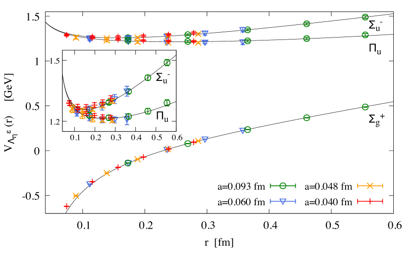
Figure 1: Lattice results for the (hybrid) static potentials.

4 Excluding possible systematic errors

4.1 Finite spatial lattice volume

When performing computations at different spatial lattice volumes for gauge group $SU(2)$ (see Ref. [28]) we observed a sizable volume dependence of the ordinary static potential and hybrid static potentials, when the volume is smaller than $\approx(1.0\,\text{fm})^{3}$. For example, shrinking the spatial lattice volume below this size causes a small negative shift for the ordinary static potential $\Sigma_{g}^{+}$, while there is a much larger positive shift for the hybrid static potential $\Pi_{u}$. For a spatial lattice volume of $(1.2\,\text{fm})^{3}$, however, as used for the computation of the potentials shown in Figure 1, these finite volume corrections are tiny and negligible compared to statistical errors.

4.2 Topological freezing

Gauge field configurations can be classified according to their topological charge. Topological freezing denotes the problem that a Monte Carlo simulation is trapped in one of the topological sectors. The gauge link configurations generated in such a simulation do not form a representative set distributed according to $e^{-S}$. This problem is typically observed when using a lattice spacing $a$ smaller than $\approx 0.05\,\text{fm}$ [29] and becomes more severe, when approaching the continuum limit, i.e. when further decreasing $a$. If a simulation is fully trapped in a topological sector, observables exhibit specific finite volume corrections in addition to those discussed in section 4.1 (see e.g. Refs. [30, 31, 32, 33]).

To check, whether our simulations suffer from topological freezing, we computed the topological charge on the gauge link configuration via a field-theoretic definition with a simple clover-leaf discretization and 4-dimensional APE-smearing [34]. In Figure 2, we show the topological charge as a function of the Monte Carlo time for two independent exemplary runs for two lattice spacings. One can see that the topological charge still changes frequently even at the smallest lattice spacing, $a=0.040\,\text{fm}$. The topological charge distribution and topological susceptibility also indicate that the Monte Carlo algorithm is able to sample the gauge link configurations correctly. Using a suitable binning and several independent Monte Carlo runs we exclude that statistical errors are underestimated because of autocorrelations, which are also expected to increase with decreasing lattice spacing. In summary, the potentials presented in this work should be free of any systematic errors from topological freezing.

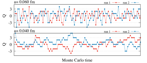
Figure 2: Topological charge as a function of the Monte Carlo time for two independent exemplary runs for two lattice spacings.

4.3 Glueball decays

For sufficiently small quark-antiquark separations $r$ the energy difference between a hybrid static potential and the ordinary static potential $\Sigma_{g}^{+}$ is large enough such that the hybrid flux tube can dissolve into a glueball and the $\Sigma_{g}^{+}$ flux tube. The minimal energy, which is necessary for such a decay into the lightest glueball with quantum numbers $J^{PC}=0^{++}$ and mass $m_{0^{++}}\approx 4.21/r_{0}$ [18] is shown as a dashed line in Figure 3 together with our lattice results for hybrid static potentials.

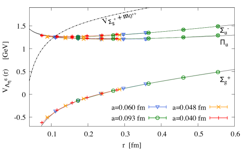
Figure 3: Threshold energy $V_{\Sigma_{g}^{+}}(r)+m_{0^{++}}$ for the decay of a hybrid flux tube to the flux tube of the ordinary static potential and the lightest $0^{++}$ glueball.

Below a critical separation, in particular below $r_{\text{crit}}\approx 0.1\,\text{fm}$ for the lowest hybrid potential $\Pi_{u}$, a $0^{++}$ glueball decay is energetically allowed and the hybrid static potential creation operator might generate non-vanishing overlap to the $\Sigma_{g}^{+}$ flux tube and the glueball. For the second lowest hybrid potential $\Sigma_{u}^{-}$ and the higher lying hybrid potential $\Sigma_{g}^{-}$ it is possible to exclude decays to the lightest $0^{++}$ glueball using symmetry arguments (we will discuss that in detail in a future publication). Still allowed are decays into the next lightest glueball with quantum numbers $J^{PC}=2^{++}$. However, this is energetically only possible at significantly smaller separations than those we investigated.

In this work, we present lattice results for the hybrid static potentials $\Pi_{u}$ and $\Sigma_{u}^{-}$ for separations below $r_{\text{crit}}\approx 0.1\,\text{fm}$. There is, however, no sign of contamination by glueball decays, since the two lowest hybrid static potentials reveal the expected upward curvature and degeneracy at small separations [12].

References

- [1] E. Braaten, C. Langmack and D.H. Smith, Selection Rules for Hadronic Transitions of XYZ Mesons, Phys. Rev. Lett. 112 (2014) 222001 [1401.7351].
- [2] C. Meyer and E. Swanson, Hybrid Mesons, Prog. Part. Nucl. Phys. 82 (2015) 21 [1502.07276].
- [3] E.S. Swanson, XYZ States: Theory Overview, AIP Conf. Proc. 1735 (2016) 020013 [1512.04853].
- [4] R.F. Lebed, R.E. Mitchell and E.S. Swanson, Heavy-Quark QCD Exotica, Prog. Part. Nucl. Phys. 93 (2017) 143 [1610.04528].
- [5] S.L. Olsen, T. Skwarnicki and D. Zieminska, Nonstandard heavy mesons and baryons: Experimental evidence, Rev. Mod. Phys. 90 (2018) 015003 [1708.04012].
- [6] N. Brambilla, S. Eidelman, C. Hanhart, A. Nefediev, C.-P. Shen, C.E. Thomas et al., The states: experimental and theoretical status and perspectives, Phys. Rept. 873 (2020) 1 [1907.07583].
- [7] S. Perantonis and C. Michael, Static potentials and hybrid mesons from pure su(3) lattice gauge theory, Nuclear Physics B 347 (1990) 854 .
- [8] K. Juge, J. Kuti and C. Morningstar, Gluon excitations of the static quark potential and the hybrid quarkonium spectrum, Nucl. Phys. B Proc. Suppl. 63 (1998) 326 [hep-lat/9709131].
- [9] K. Juge, J. Kuti and C. Morningstar, Ab initio study of hybrid anti-b g b mesons, Phys. Rev. Lett. 82 (1999) 4400 [hep-ph/9902336].
- [10] E. Braaten, C. Langmack and D.H. Smith, Born-Oppenheimer Approximation for the XYZ Mesons, Phys. Rev. D 90 (2014) 014044 [1402.0438].
- [11] S. Capitani, O. Philipsen, C. Reisinger, C. Riehl and M. Wagner, Precision computation of hybrid static potentials in SU(3) lattice gauge theory, Phys. Rev. D 99 (2019) 034502 [1811.11046].
- [12] M. Berwein, N. Brambilla, J. Tarrús Castellà and A. Vairo, Quarkonium Hybrids with Nonrelativistic Effective Field Theories, Phys. Rev. D 92 (2015) 114019 [1510.04299].
- [13] R. Oncala and J. Soto, Heavy Quarkonium Hybrids: Spectrum, Decay and Mixing, Phys. Rev. D96 (2017) 014004 [1702.03900].
- [14] N. Brambilla, W.K. Lai, J. Segovia, J. Tarrús Castellà and A. Vairo, Spin structure of heavy-quark hybrids, Phys. Rev. D 99 (2019) 014017 [1805.07713].
- [15] N. Brambilla, W.K. Lai, J. Segovia and J. Tarrús Castellà, QCD spin effects in the heavy hybrid potentials and spectra, Phys. Rev. D 101 (2020) 054040 [1908.11699].
- [16] S. Perantonis, A. Huntley and C. Michael, Static potentials from pure su(2) lattice gauge theory, Nuclear Physics 326 (1989) 544.
- [17] K.J. Juge, J. Kuti and C.J. Morningstar, A Study of hybrid quarkonium using lattice QCD, AIP Conf. Proc. 432 (1998) 136 [hep-ph/9711451].
- [18] C.J. Morningstar and M.J. Peardon, The Glueball spectrum from an anisotropic lattice study, Phys. Rev. D60 (1999) 034509 [hep-lat/9901004].
- [19] K.J. Juge, J. Kuti and C. Morningstar, Fine structure of the QCD string spectrum, Phys. Rev. Lett. 90 (2003) 161601 [hep-lat/0207004].
- [20] G.S. Bali and A. Pineda, QCD phenomenology of static sources and gluonic excitations at short distances, Phys. Rev. D 69 (2004) 094001 [hep-ph/0310130].
- [21] K.J. Juge, J. Kuti and C. Morningstar, Excitations of the static quark anti-quark system in several gauge theories, in International Conference on Color Confinement and Hadrons in Quantum Chromodynamics - Confinement 2003, 2003, DOI [hep-lat/0312019].
- [22] O. Philipsen, C. Pinke, A. Sciarra and M. Bach, CL2QCD - Lattice QCD based on OpenCL, PoS LATTICE2014 (2014) 038 [1411.5219].
- [23] M. Lüscher and P. Weisz, Locality and exponential error reduction in numerical lattice gauge theory, JHEP 09 (2001) 010 [hep-lat/0108014].
- [24] S. Necco and R. Sommer, The N(f) = 0 heavy quark potential from short to intermediate distances, Nucl. Phys. B 622 (2002) 328 [hep-lat/0108008].
- [25] ETM collaboration, The Static-light meson spectrum from twisted mass lattice QCD, JHEP 12 (2008) 058 [0810.1843].
- [26] S. Necco, The Static quark potential and scaling behavior of SU(3) lattice Yang-Mills theory, phd thesis, 2003. hep-lat/0306005.
- [27] N. Brambilla, A. Pineda, J. Soto and A. Vairo, Potential NRQCD: An Effective theory for heavy quarkonium, Nucl. Phys. B 566 (2000) 275 [hep-ph/9907240].
- [28] C. Riehl and M. Wagner, Hybrid static potentials in SU(2) lattice gauge theory at short quark-antiquark separations, in Asia-Pacific Symposium for Lattice Field Theory, 2020 [2008.12216].
- [29] M. Lüscher and S. Schaefer, Lattice QCD without topology barriers, JHEP 07 (2011) 036 [1105.4749].
- [30] R. Brower, S. Chandrasekharan, J.W. Negele and U. Wiese, QCD at fixed topology, Phys. Lett. B 560 (2003) 64 [hep-lat/0302005].
- [31] S. Aoki, H. Fukaya, S. Hashimoto and T. Onogi, Finite volume QCD at fixed topological charge, Phys. Rev. D 76 (2007) 054508 [0707.0396].
- [32] A. Dromard and M. Wagner, Extracting hadron masses from fixed topology simulations, Phys. Rev. D 90 (2014) 074505 [1404.0247].
- [33] W. Bietenholz, C. Czaban, A. Dromard, U. Gerber, C.P. Hofmann, H. Mejía-Díaz et al., Interpreting Numerical Measurements in Fixed Topological Sectors, Phys. Rev. D93 (2016) 114516 [1603.05630].
- [34] K. Cichy, A. Dromard, E. Garcia-Ramos, K. Ottnad, C. Urbach, M. Wagner et al., Comparison of different lattice definitions of the topological charge, PoS LATTICE2014 (2014) 075 [1411.1205].