Collective excitations of rotating dusty plasma under quasilocalized charge approximation of strongly coupled systems

Abstract

Collective excitations of rotating dusty plasma are analyzed under the quasi localized charge approximation (QLCA) framework for strongly coupled systems by explicitly accounting for the dust rotation in the analysis. Considering the firm analogy of magnetoplasmons with “rotoplasmons” established by the recent rotating dusty plasma experiments, the relaxation introduced by the rotation in their strong coupling and 2-dimensional (often introduced by gravitational sedimentation) characteristics is emphasized in their dispersion. Finite rotation version of both strong and weak coupling dispersions is derived and analyzed, showing correspondence between a ‘faster rotating but weakly coupled’ branch and its strongly coupled counterpart, relevant to both magnetized and unmagnetized dust experiments, in gravity or microgravity conditions. The first correspondence between their measurements in rotating plasmas and the QLCA produced dispersions in a rotating frame, with an independent numerical validation, is presented in detail.

I Introduction

Collective excitations in systems with strongly interacting charged particle constituents are fundamental to understanding the evolution of many physical systems, including planetary systems (Yaroshenko et al., 2007, 2009; Shukla et al., 2003), accretion disks (Nekrasov, 2009), binary stars and ultra dense crust of the neutron stars (Chabrier et al., 2002). Strongly coupled phase of matter efficiently models physical state of not only astrophysical systems such as ion fluid in white dwarfs (Koester and Schönberner, 1986), neutron star exteriors but also many laboratory scale systems that are dynamically close to them, such as localized ions(Willitsch et al., 2008) in extended cryogenic traps or heavily charged dust grains (Pramanik et al., 2002; Quinn and Goree, 2000) suspended in electron-ion plasmas.

While the rotation is an inseparable ingredient of dynamics of most of the astrophysical systems, interplay of rotation with extremely large magnetic field present in them provides vital clues about their dynamical state as well as their internal structure, for example pulsating radiations from pulsars because of misaligned magnetic and rotational axes (Ghosh, 2007) that led to their discovery Hewish et al. (1968). Achieving the magnetization of heavier species in strongly coupled system realized in normal laboratory conditions remains a considerable challenge. For example, the dusty plasma experiments where observable dust magnetization needs considerably high magnetic field Uchida et al. (2004), hence dedicated facilities to achieve this goal Thomas et al. (2015, 2012). A remarkable dynamical analogy between the effects of rotation and magnetization in such systems although exists and is illustrated in some recent laboratory dusty plasmas experiments where an “effective magnetization” resulted from an induced dust rotation Kählert et al. (2012). As estimated, for example, by Kählert et al. (Kählert et al., 2012), a rotation frequency of about 10 Hz in a typical dusty plasma (dust charge $\sim 10^{4}e$ and mass$\sim 10^{-12}$ kg) generates effects equivalent to magnetic field exceeding $10^{4}$ T. Advanced experiments with dust rotation have also demonstrated excitation of dust magnetoplasmons in such “effectively magnetized” dust components Hartmann et al. (2013). Addressing the analytical approach to these results, by explicitly admitting dust rotation in one of the standard dynamical models of strongly coupled systems, and their quantitative comparison with the experimentally observed dispersion is the subject of the present paper. The analysis also applies to perturbations of general equilibrium dust vortex solutions in unmagnetized kaur et al. (2015) as well as weakly magnetized plasma conditions Kumar and Sharma (2020).

The collective excitations in strongly to weakly coupled systems are widely formulated and studied under the quasi-localized-charge approximation (QLCA) approach Golden and Kalman (2000); Kalman and Golden (1990); Golden et al. (1992). The QLCA formulation appropriately reduces into usual fluid formulation under a random phase approximation (RPA) regime Golden and Kalman (2000); Hou et al. (2009). Strong coupling effects in presence of a magnetic field have also been addressed under the QLCA formulation (Kalman and Golden, 1990; Jiang et al., 2007), indicating that its results may be applicable to the “effectively magnetized” dusty plasmas.

Essential to the characterization of collective excitations of effective magnetoplasmons is to ascertain their dispersion, as observed in the experiments, against the analytic dispersion relation produced by the theory of strongly coupled rotating dust system. An existing QLCA approach that considered dust interacting by Yukawa interaction was done by Jiang et al.(Jiang et al., 2007) who also considered magnetic field and therefore is relevant to the cases with dust rotation. The result from the Jiang et al. however showed that the agreement of magnetized QLCA results with computer simulations is achievable for strongly coupled limit solutions. Specifically, the saturation displayed in the frequency of the dispersive excitation at larger wave numbers remained achievable only for strong coupling and is absent for 2D RPA limit. In somewhat contrast, the saturation is measured with relatively weak coupling (liquid phase) regime in the recent “effectively magnetized” rotating dusty plasma experiment Hartmann et al. (2013) and also in the corresponding computer simulations, both of which were interpreted based on existing QLCA approaches.

Of the immediate interest therefore is to workout a QCLA formulation which explicitly accounts for dust rotation in a Yukawa system, and also derive its limiting cases, for example, that of the weakly coupled (or RPA) limit where it yields equivalence to the regular explicitly rotating “dust fluid” formulation, which is done in this paper. Not limiting our analysis to characterizing the analytically obtained dispersion relations, we also compute the multi-component rotating dust fluid model solutions, producing their independent agreement with analytical dispersions, thus simultaneously validating the accuracy of the analytical results.

The analytical and numerical analysis of the rotating plasma dispersion presented here shows that if the weakly coupled limit is considered with distant axial boundaries (3D effects), the frequency saturation not only becomes achievable in the rotating dusty plasma but the saturated frequency values also show quantitative agreement with those recovered in the recent experiments of the rotating dusty plasmas Hartmann et al. (2013). This behavior indicates that a dust medium with large enough coupling parameter $\Gamma$, when driven to a nonequilibrium state by an external rotation, not only displays weak coupling like effects but also a relaxation from the boundary effects such that the plasma bulk strongly limited by axial boundaries still displays nearly 3D characteristics. The rotation of the dust thus additionally appears to relax the 2D effects (2D sedimentation, usually generated by the gravity(Khrapak et al., 2016a)) on the dust cloud. It is therefore concluded that this nonequilibrium rotating system not only shows isomorphism with magnetized dust regime but perhaps also with its microgravity regime, rendering the latter realizable also in the regular ground based laboratory experiments, if dust is subjected to a rotation. The analysis therefore motivate studies both in magnetized as well as in microgravity conditions in order to examine their similarity with ground based rotating dusty plasma experiments. The analysis may thus serve as a link between ground based magnetized dusty plasma experiments, like MDPX, and the International Space Station (ISS) based experiments in microgravity conditions (Pustylnik et al., 2016; Fortov et al., 2003; Khrapak et al., 2016a).

The present paper is organized as follows. The QLCA formulation, explicitly accounting dust rotation, is developed in the Sec. II. The first characterization of dispersion relation for a strongly coupled rotating dusty plasma with Yukawa interaction is also done in Sec.II showing a tendency in RPA limit rotating dust dispersion to increasingly agree with the strongly coupled dispersion at stronger rotation. The RPA limit dispersions are shown recoverable from a multi-component model with rotating dust fluid in Sec. IIA. This model is solved numerically to validate the characterization of the RPA limit dispersion relation which is done using the set of parameter derived from recent rotating dusty plasma experiment in Sec. IIIB. A general characterization of the dispersion, independent of the experimental parameter sets, is presented in Sec. IIIC with respect to variation in rotation frequency and screening by the background plasma. Finally, the issue of strongly coupled rotating dust in experiments showing better agreement with RPA limit dispersion with increasing rotation frequency is addressed qualitatively in Sec.IIID.

II The quasi-localized-charge approximation (QLCA) for rotating dusty plasma

The QLCA (quasi-localized-charge approximation) is very general microscopic model for the description of linear dielectric response and collective mode dispersion in strongly coupled systems. It assumes that charge particles, in strongly coupled system, are quasi-localized around the equilibrium position in corresponding potential wells and respond linearly to small external perturbing fields. Our approach to analyze the spectral properties is aimed to address the laboratory experiments having rotating dust component Hartmann et al. (2013). The strongly coupled dusty plasma in QLCA approach is well represented by a one component plasma with strong particle charge, namely, the dust, in a Yukawa potential produced by the shielding effect of the background electron and ion species. As in the non-rotating QLCA treatment Golden and Kalman (2000), we begin by writing the microscopic equation of motion for the single particle, in the absence of external force and collisions, however in the frame rotating with the dust cloud. We therefore consider a local coordinate system in the dust cloud such that the axis of rotation is aligned to $\hat{z}$. We write our microscopic equation of motion of the dust particle located at the position $r_{i}$, for the component $r_{i\mu}$ aligned to the direction $\mu~{}(=x,y)$,

$$\begin{split}m_{\rm d}\frac{\partial^{2}{r}_{i\mu}}{\partial t^{2}}=\sum_{j}{K}_{ij\mu\nu}r_{j\nu}-2m_{\rm d}\left[{\bf\Omega}\times\frac{\partial{\bf r}_{i}}{\partial t}\right]_{\mu}\\ -m_{\rm d}[{\bf\Omega}\times({\bf\Omega}\times{\bf r}_{i})]_{\mu}-\frac{\partial V}{\partial r_{\mu}}=0,\end{split}$$ (1)

where second and third terms in right hand side are Coriolis force and centrifugal force, respectively. The quantity $V$ is the confinement potential whose gradient along $\mu$ balances the corresponding component of the centrifugal force in the typical equilibrium condition Nekrasov (2009). The dynamical tensor $K_{ij\mu\nu}$, with dimension index $\mu,\nu=x,y,z$ (index $i,j$ only enumerate particles), represents the effect of the inter-particle interaction in a Yukawa system which, in the non-retarded limit (velocity of electromagnetic waves $c\rightarrow\infty$) is given by Kalman and Golden (1990),

$$K_{ij\mu\nu}=(1-\delta_{ij})\frac{\partial^{2}}{\partial r_{i\mu}\partial r_{j\nu}}\phi(|{\bf r}_{i}-{\bf r}_{j}|)$$ (2)

$$-\delta_{ij}\left\{\sum_{l=1}^{N}(1-\delta_{il})\frac{\partial^{2}}{\partial r_{i\mu}\partial r_{l\nu}}\phi(|{\bf r}_{i}-{\bf r}_{l}|)\right.$$ (3)

$$\left.+\int d^{2}r^{\prime}\frac{\partial^{2}}{\partial r_{i\mu}\partial{r^{\prime}_{\nu}}}\frac{\rho_{\rm b}({\bf r^{\prime}})}{\rho_{0}}\phi(|{\bf r}_{i}-{\bf r^{\prime}}|)\right\},$$ (4)

where $\rho_{\rm b}({\bf r^{\prime}})$ is the charge density of the background plasma, $\rho_{0}$ is unperturbed dust charge density and potential $\phi$ has the form,

$$\phi(|{\bf r}_{i}-{\bf r}_{j}|)=e^{-\kappa_{b}|{\bf r}_{i}-{\bf r}_{j}|}\frac{Z^{2}e^{2}}{|{\bf r}_{i}-{\bf r}_{j}|},$$ (5)

with

$$\kappa_{b}^{2}=\sum_{A}4\pi Z_{A}^{2}e^{2}n_{A}\beta_{A}.$$ (6)

The subscript $A$ corresponds the species in the background plasma, specifically electron and ions in a typical dusty plasma. In its Fourier transformed form, the potential $\phi({\bf r-r^{\prime}})$ therefore reads,

$$\phi(k)=\frac{4\pi Z^{2}e^{2}}{k^{2}+\kappa_{b}^{2}}.$$ (7)

We now consider a small perturbation $\xi_{i\mu}$ of the equilibrium location $r_{i\mu}$ in order to explore the linear wave-like response of the system. Accordingly, the Eq. (1) in the frequency domain, obtained by the Fourier transformation is,

$$\begin{split}-m_{\rm d}\omega^{2}\xi_{i\mu}(\omega)-\sum_{j}K_{ij\mu\nu}\xi_{j\nu}(\omega)-i\omega 2m_{\rm d}~{}\epsilon_{\nu\delta\mu}{\Omega_{\nu}}{\xi}_{i\delta}(\omega)\\ =ZeE_{\mu}(\xi_{i\mu},\omega).\end{split}$$ (8)

Note that $K_{ij\mu\nu}$ is independent of $\omega$ in the non-retarded limit and $\epsilon_{\nu\delta\mu}{\Omega_{\nu}}{\xi}_{i\delta}(\omega)$ represents the cross product ${\bf\Omega}\times{\bf\xi}_{i}(\omega)$ in the index notation, with $\epsilon_{\nu\delta\mu}$ having its conventional values with respect to the order $\mu\nu\delta$ of the indices, each taking values $x,y$ and $z$, respectively. Summation is implied over the repeated indices. Considering that the 2D problem is solved in the plane perpendicular to ${\bf\Omega}$ (aligned to $\hat{z}$) and corotating with the dust, as described by schematic Fig. 1, the index $\mu$ takes only two values, $x$ and $y$, hence the cross product contributes only one term containing $\delta\neq\nu,\mu$.

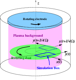
Figure 1: Schematic of the rotating dusty plasma setup. The rectangular simulation zone located in the frame co-rotating with the dust, is drawn at time $t$ (solid line) and at quarter of the rotation period after time $t$ (dotted line) in the laboratory frame.

Considering their spatially extended distribution, displacements $\xi_{i}(\omega)$ can now be Fourier expanded in the series of vectors ${\bf q}$ as,

$$\begin{split}\xi_{i}(\omega)=\frac{1}{\sqrt{Nm_{d}}}\sum_{\bf q}\xi_{\bf q}(\omega)e^{i{\bf q}\cdot{\bf r}_{i}}.\end{split}$$ (9)

Similarly, expression of $K_{ij\mu\nu}$ in these terms Kalman and Golden (1990) would be,

$$K_{ij\mu\nu}=\frac{1}{V_{dD}}\sum_{\bf q}q_{\mu}q_{\nu}\psi_{dD}({\bf q},\omega)[e^{i{\bf q}\cdot({\bf r}_{i}-{\bf r}_{j})}$$

$$-\delta_{ij}e^{i{\bf q}\cdot{\bf r}_{i}}n_{q}+\delta_{ij}\frac{n_{b{\bf q}}Z_{b}}{Z}e^{i{\bf q}\cdot{\bf r_{i}}}].$$ (10)

Using the dusty plasma quasi-neutrality condition we get $n_{b}Z_{b}=NZ$, where $Z_{b}$ is average charge per part in the background continuum if it is divided into same number of parts as the number of dust particles $N$. Additionally, if the background plasma has no spatial structures, the factor $e^{i{\bf q}\cdot{\bf r_{i}}}$ reduces to $\delta_{\bf q}$ and $n_{b{\bf q}}$ becomes independent of ${\bf q}$. Using these two conditions, the definition (10) reduces to,

$$K_{ij\mu\nu}=\frac{1}{V_{dD}}\sum_{\bf q}q_{\mu}q_{\nu}\psi_{dD}({\bf q},\omega)[e^{i{\bf q}\cdot({\bf r}_{i}-{\bf r}_{j})}$$

$$-\delta_{ij}e^{i{\bf q}\cdot{\bf r}_{i}}n_{q}+N\delta_{ij}\delta_{\bf q}],$$ (11)

where the subscript $dD$ in $V$ and $\psi$ defines the dimensionality of the system by takes values $dD=2D,3D$. The general definition of the potential $\psi_{dD}$ is Golden and Kalman (2000),

$$\psi_{dD}(q,\omega)=\left[1-\left(\frac{\omega^{2}}{q^{2}c^{2}}\right)\right]^{(3-d)/2}\phi_{dD}(\omega),$$ (12)

such that in 3D, $\psi_{3D}=\phi_{3D}$.

In order to examine an excitation with vector ${\bf k}$ in the dust cloud, we follow the standard QLCA prescription Golden and Kalman (2000) and substitute (9), (10), into Eq. (8), multiply it with $\exp{(-i{\bf k}\cdot{\bf r}_{i})}$ (Note that $n_{\bf k}=\sum_{i}\exp{(-i{\bf k}\cdot{\bf r}_{i})}$) and sum over $i$, for $N$ particles. This sequence of operations produces,

$$\begin{split}-m_{\rm d}\omega^{2}\sum_{\bf q}\xi_{{\bf q}\mu}(\omega)n_{k-q}\\ -\frac{1}{V_{dD}}\sum_{\bf q,p}q_{\mu}q_{\nu}\psi_{dD}({\bf q},\omega)[n_{k-q}n_{q-p}\\ -n_{k-q-p}n_{q}+N\delta_{q}n_{k-p}]\xi_{\bf p\nu}(\omega)\\ +2i\omega m_{\rm d}~{}\epsilon_{\nu\delta\mu}\Omega_{\nu}\sum_{\bf q}\xi_{\bf q\delta}(\omega)n_{k-q}\\ =Zen\sqrt{\frac{m_{d}}{N}}\sum_{\bf q}E_{\bf q}(\xi_{\bf q\mu},\omega)n_{k-q}.\end{split}$$ (13)

We now apply the central assumption of QLCA formulation and replace the quantities $n_{k-q},n_{k-q}n_{p-q}$ and $n_{k-q-p}n_{q}$ by their ensemble averages,

$$\langle{n_{\bf k-q}}\rangle = N\delta_{\bf k-q},$$ (14)

$$\langle{n_{\bf k-q}n_{\bf q-p}}\rangle = NS(|{\bf k-q}|)\delta_{\bf k-p}+N^{2}\delta_{\bf k-q}\delta_{\bf q-p},$$ (15)

$$\langle{n_{\bf k-p-q}n_{\bf q}}\rangle = NS(|{\bf q}|)\delta_{\bf k-p}+N^{2}\delta_{\bf q}\delta_{\bf k-p},$$ (16)

where $S({\bf q})$ is static structure function. In the last step, we substitute these ensemble averages into the respective terms and sum over indices, wherever possible, As a result the equation further becomes,

$$\begin{split}-m_{\rm d}\omega^{2}\xi_{{\bf k}\mu}(\omega)\\ -\frac{N}{V_{dD}}k_{\mu}k_{\nu}\psi_{dD}({\bf k},\omega)\xi_{\bf k\nu}(\omega)\\ -\frac{1}{V_{dD}}\sum_{\bf q}q_{\mu}q_{\nu}\psi_{dD}({\bf q},\omega)\\ \times[S(|{\bf k-q}|)-S(|{\bf q}|)]\xi_{\bf k\nu}(\omega)\\ +2i\omega m_{\rm d}~{}\epsilon_{\nu\delta\mu}\Omega_{\nu}\xi_{\bf k\delta}(\omega)\\ =Zen\sqrt{Nm_{d}}E_{\bf k}(\xi_{\bf k\mu},\omega).\end{split}$$ (17)

This, in absence of external electric field $E$, yields a macroscopic equation for $\xi_{{\bf k}\nu}$ of the form,

$$[\omega^{2}\delta_{\mu\nu}-C_{\mu\nu}({\bf k},\omega)]\xi_{{\bf k}\nu}(\omega)+2i\omega~{}\epsilon_{\nu\delta\mu}\Omega_{\nu}\xi_{\bf k\delta}(\omega)$$

$$=0.$$ (18)

Which can be written in a more general form as,

$$[\omega^{2}\delta_{\mu\nu}+2i\omega~{}\epsilon_{\mu\nu\delta}\Omega_{\delta}-C_{\mu\nu}({\bf k},\omega)]\xi_{{\bf k}\nu}(\omega)=0,$$ (19)

where, for the present non-retarded limit we define,

$$D_{\mu\nu}({\bf k})=\frac{1}{m_{\rm d}V_{dD}}\sum_{\bf q}q_{\mu}q_{\nu}\psi(q)[S(|{\bf k-q}|)-S(q)].$$ (20)

Allowing us to write,

$$C_{\mu\nu}({\bf k},\omega)=\omega_{\rm pd}^{2}\left[\frac{k_{\mu}k_{\nu}}{k^{2}+\kappa_{b}^{2}}+\cal{D}_{\mu\nu}({\bf k},\omega)\right].$$ (21)

where the dimensionless form of $D_{\mu\nu}$ is used,

$${\cal D}_{\mu\nu}({\bf k}) = \sum_{\bf q}\frac{q_{\mu}q_{\nu}}{q^{2}+\kappa_{b}^{2}}[\tilde{S}(|{\bf k-q}|)-\tilde{S}(q)].$$ (22)

In non-retarded limit, the only surviving transverse mode is via a transverse shear. This is indeed recovered from ${\cal D}_{\mu\nu}(\bf k)$ which contains both longitudinal and transverse shear. The longitudinal component of ${\cal D}_{\mu\nu}$ is recovered by operating ${\cal D}_{\mu\nu}({\bf k})$ over with longitudinal projection tensor ${\cal L}_{\mu\nu}({\bf k})={k_{\mu}k_{\nu}}{/k^{2}}$,

$${\cal D}_{L}({\bf k}) = \sum_{\bf q}{\cal L}_{\mu\nu}({\bf k})\frac{q_{\mu}q_{\nu}}{q^{2}+\kappa_{b}^{2}}[\tilde{S}(|{\bf k-q}|)-\tilde{S}(q)],$$ (23)

or,

$${\cal D}_{L}({\bf k}) = \sum_{\bf q}\frac{({\bf k\cdot q})^{2}}{k^{2}(q^{2}+\kappa_{b}^{2})}[\tilde{S}(|{\bf k-q}|)-\tilde{S}(q)].$$ (24)

Similarly, the transverse component of ${\cal D}_{\mu\nu}$ is recovered by operating it over by the transverse projection tensor $\frac{1}{2}{\cal T}_{\mu\nu}({\bf k})=\frac{1}{2}(\delta_{\mu\nu}-k_{\mu}k_{\nu}/k^{2})$,

$${\cal D}_{T}({\bf k})=\sum_{\bf q}\frac{1}{2}\{\delta_{\mu\nu}-{\cal L}_{\mu\nu}({\bf k})\}\frac{q_{\mu}q_{\nu}}{q^{2}+\kappa_{b}^{2}}$$

$$\times[\tilde{S}(|{\bf k-q}|)-\tilde{S}(q)].$$ (25)

Since, the contribution in transverse component comes only from non-diagonal terms this can be readily written as,

$${\cal D}_{T}({\bf k})=\sum_{\bf q}-\frac{1}{2}{\cal L}_{\mu\nu}({\bf k})\frac{q_{\mu}q_{\nu}}{q^{2}+\kappa_{b}^{2}}[\tilde{S}(|{\bf k-q}|)-\tilde{S}(q)].$$ (26)

In 3D conditions, the relation between ${\cal D}_{L}({\bf k})$ and ${\cal D}_{T}({\bf k})$ becomes Golden and Kalman (2000),

$${\cal D}_{T}({\bf k}) = -\frac{1}{2}{\cal D}_{L}({\bf k}).$$ (27)

We now find the dispersion relation by allowing the determinant to vanish for nontrivial solutions Golden et al. (1993),

$$\det[\omega^{2}\delta_{\mu\nu}+2i\omega~{}\epsilon_{\mu\nu\delta}\Omega_{\delta}-C_{\mu\nu}({\bf k},\omega)]=0,$$ (28)

which, up on substituting the elements of matrix $C_{\mu\nu}$ and considering ${\bf\Omega}=\Omega\hat{z}$, becomes,

$$\left[\omega^{2}-\left\{\omega_{0}^{2}({\bf k})+D_{L}({\bf k})\right\}\right]\left[\omega^{2}-D_{T}({\bf k})\right]$$

$$-\omega^{2}(2\Omega)^{2}=0,$$ (29)

where, $\omega_{0}^{2}({\bf k})=\omega_{\rm pd}^{2}{k^{2}}{/(k^{2}+\kappa_{b}^{2})}$, such that solutions of Eq. (29) are,

$$\omega^{2}({\bf k})=\frac{1}{2}[\{\omega_{0}^{2}({\bf k})+D_{L}({\bf k})+D_{T}({\bf k})\}+(2\Omega)^{2}]$$

$$\pm\frac{1}{2}\left([\{\omega_{0}^{2}({\bf k})+D_{L}({\bf k})+D_{T}({\bf k})]+(2\Omega)^{2}\}^{2}\right.$$

$$\left.-4D_{T}({\bf k})[\omega_{0}^{2}({\bf k})+D_{L}({\bf k})]\right)^{1/2},$$ (30)

yielding, in the case $\Omega\rightarrow 0$, the well known frequencies for longitudinal and transverse modes,

$$\omega_{L}({\bf k}) = [\omega_{0}^{2}({\bf k})+D_{L}({\bf k})]^{1/2}$$ (31)

$$\omega_{T}({\bf k}) = [D_{T}({\bf k})]^{1/2}.$$ (32)

It is now possible to examine the general QLCA dispersion (30) which accommodates all the essential effects for this setup, namely, the strong coupling ($D_{\mu\nu}\neq 0$), the Yukawa potential and the dust rotation. The strong coupling effects can be included in their simplest form by adopting the long wavelength limit $\Omega a/c\ll ka\ll 1$, or the “excluded volume consideration” (Khrapak et al., 2016b) where $D_{L,T}$ take a relatively approximate but simpler analytic form, given by,

$$D_{L,T}({\bf k})=\omega_{\rm pd}^{2}\int_{0}^{\infty}dr\frac{e^{-\kappa r}}{r}[g(r)-1]{\cal K}_{L,T}(kr,\kappa r),$$ (33)

where,

$${\cal K}_{L}(kr,\kappa r)=-2\left[1+\kappa r+\frac{1}{3}(\kappa r)^{2}\right]$$

$$\times\left[\frac{\sin{kr}}{kr}+3\frac{\cos{kr}}{(kr)^{2}}-3\frac{\sin{kr}}{(kr)^{3}}\right]$$

$$+\frac{1}{3}(\kappa r)^{2}\left(\frac{\sin{kr}}{kr}-1\right),$$ (34)

and

$${\cal K}_{T}(kr,\kappa r)=\left[1+\kappa r+\frac{1}{3}(\kappa r)^{2}\right]$$

$$\times\left[\frac{\sin{kr}}{kr}+3\frac{\cos{kr}}{(kr)^{2}}-3\frac{\sin{kr}}{(kr)^{3}}\right]$$

$$-\frac{1}{3}(\kappa r)^{2}\left(\frac{\sin{kr}}{kr}-1\right).$$ (35)

The function $g(r)$ in this limit is approximated to a step-like function, having uniform strength 1 in the region beyond a minimum radius $R$ and remaining zero within the region $r<R$, allowing longitudinal and transverse mode frequencies to be recovered, respectively, as,

$$\omega_{L}^{2}=(2\Omega)^{2}+\omega_{\rm pd}^{2}e^{-kR}\left[(1+kR)\left(\frac{1}{3}-\frac{2\cos{kR}}{k^{2}R^{2}}\right.\right.$$

$$\left.\left.+\frac{2\sin{kR}}{k^{3}R^{3}}\right)-\frac{\kappa^{2}}{\kappa^{2}+k^{2}}\left(\cos{kR}+\frac{\kappa}{k}\sin{kR}\right)\right.$$

$$\left.+(1+kR)\left(\frac{1}{3}-\frac{\cos{kR}}{(kR)^{2}}+\frac{\sin{kR}}{(kR)^{3}}\right)\right.$$

$$\left.\times\frac{(2\Omega)^{2}}{(2\Omega)^{2}+\omega^{2}_{0}}\right],$$ (36)

and

$$\omega_{T}^{2}=\frac{\omega^{2}_{0}\omega_{\rm pd}^{2}e^{-kR}(1+kR)}{(2\Omega)^{2}+\omega^{2}_{0}}\left[\frac{1}{3}-\frac{\cos{kR}}{(kR)^{2}}+\frac{\sin{kR}}{(kR)^{3}}\right].$$ (37)

These dispersion relations are plotted in Fig. 2, along with the RPA (or Vlasov) approximated version of $\omega_{L}(k)$. For computing $\omega_{L,T}(k)$ plotted in Fig. 2, we have used $\kappa=1$, $\Gamma=180$, and $R=1+\kappa/10$ approximately, following (Khrapak et al., 2016b; Khrapak, 2017), while using $\beta$ as a variable having values 0.3 - 1.0 in order to account for the additional effect of rotation present in our expressions.

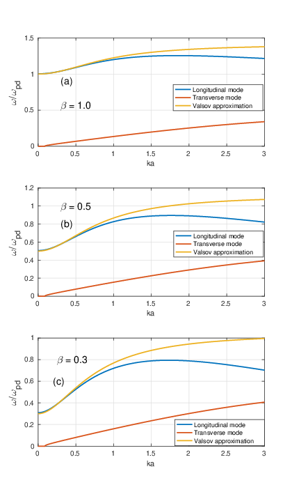
Figure 2: Longitudinal and transverse dispersion relations $\omega_{L}(k)$ and $\omega_{T}(k)$ plotted in (a), (b) and (c) for varying strength of rotation $\beta$=1, 0.5 and 0.3, respectively.

One of the most notable features of $\omega_{L,T}(k)$ is the reducing difference between the saturated values of RPA approximated version of $\omega_{L}(k)$ and its strongly coupled version, with increasing $\Omega$. The latter essentially oscillates about a saturation value as generally prescribed by the QLCA formulation. This similarity of the solutions at stronger rotation is discussed further in the context of experimental results which are compared to RPA limit dispersion in Sec. IIIB and show good agreement. As another notable feature, an onset exists in the transverse mode frequency with respect to small $k$ values where the first non-zero frequency corresponds to a minimum value of $k$. This onset was recovered and discussed in larger detail in the recent important studies of QLCA dispersion in Yukawa systems (Khrapak et al., 2019). Before characterizing the solutions, we briefly show that the RPA limit is indeed analogous to the fluid limit by obtaining the same results using a multi-component fluid model, or in the weakly coupled limit, $D_{L,T}\rightarrow 0$, of the QLCA formulation. The applied multi-component fluid model is used also for producing numerical solutions, in order to generate independent validation of the RPA results in Sec. IIIB.

II.1 The corresponding multi-component fluid model

We now use the set of 2D fluid equations, in a rotating non-inertial frame of reference, in order to model the weakly coupled rotating dusty plasma where the Coriolis force takes over the role of the Lorentz force. Here, the dust fluid equilibrium is assumed to be a rigid body like rotation of the dusty plasma with an angular frequency ${\bf\Omega}$ pointing along $\hat{z}$. The components of momentum equation for rotating isothermal dusty fluid in the x-y plane then have the following form,

$$\frac{\partial{u}_{{\rm d}x}}{\partial t}+({\bf u}_{{\rm d}}\cdot\nabla){u}_{{\rm d}x}=\frac{q_{\rm d}}{m_{\rm d}}{E}_{x}+2{u}_{dy}{\Omega},$$ (38)

$$\frac{\partial{u}_{{\rm d}y}}{\partial t}+({\bf u}_{{\rm d}}\cdot\nabla){u}_{{\rm d}y}=\frac{q_{\rm d}}{m_{\rm d}}{E}_{y}-2{u}_{{\rm d}x}{\Omega},$$ (39)

where $u_{dx}$ and $u_{dy}$ are the dust velocity along x and y-direction, respectively, $q_{\rm d}=-Z_{\rm d}e$ is the dust charge and the electric field ${\bf E}=-\nabla\phi$. The centrifugal force is once again assumed to be balanced by the force due to the confining potential with the angular frequency ${\bf\Omega}$ of the rotation radially uniform. The continuity equation for the dust is,

$$\frac{\partial n_{\rm d}}{\partial t}+\nabla\cdot n_{d0}\textbf{u}_{\rm d}=0.$$ (40)

For the low frequency wave phenomena of the dust medium, the background ions and electrons densities are well model by the Boltzmann relation,

$$n_{\rm e}=n_{{\rm e}0}\exp\left({\frac{e\phi}{k_{B}T_{\rm e}}}\right),$$ (41)

$$n_{\rm i}=n_{{\rm i}0}\exp\left({\frac{-e\phi}{k_{B}T_{\rm i}}}\right).$$ (42)

The set of equations is completed by the Poisson equation,

$$\frac{\partial^{2}\phi}{\partial x^{2}}=-4\pi e\left[n_{\rm i}-n_{\rm e}-Z_{\rm d}n_{\rm d}\right],$$ (43)

with the following equilibrium charge neutrality condition in this three component plasma,

$$n_{{\rm i}0}e=-n_{{\rm e}0}e-Z_{\rm d}en_{{\rm d}0}.$$ (44)

For a small amplitude, plane-wave-like, pure electrostatic perturbation, such that ${\bf k\|u}$, combining the linear form of Eq. (39)-(44) readily yields the same dispersion relation as Eq. (31),

$$\omega^{2}=\left(2\Omega\right)^{2}+\left[\frac{\omega^{2}_{\rm pd}}{1+{(k\lambda_{\rm i})^{-2}}+{(k\lambda_{\rm e})^{-2}}}\right],$$ (45)

although limited to response of dust to only the longitudinal (compressible) component of the initial perturbation because of the choice ${\bf k\|u}$. Note that an independently propagating pure transverse perturbation is only realizable in $\Omega\rightarrow 0$ limit and is ruled out in the presence of rotation as the transverse and longitudinal velocity components are coupled by the rotation. Recovery of dispersion (45) shows that the RPA limit of the QLCA formulation suitably represents the fluid limit of the dust response, also for the rotating dusty plasma system, considered in the above general treatment.

III Rotating dusty plasma dispersion in RPA limit and its numerical validation

In order to obtain the wave-like solutions of rotating dusty fluid perturbations, governed by the linear form of Eq. (39)-(44), we have used the pseudo-spectral technique for two dimensional solutions in (x-y) plane, perpendicular to the direction of the angular frequency ${\bf\Omega}$ in pure Cartesian geometry. The solutions thus represent excitations obtained in a frame co-rotating with the dusty plasma, hence can be suitably compared with the dispersion relations (31) and (45) derived in the same non-inertial frame of reference.

III.1 Numerical scheme and normalization

In our numerical procedure the spatial and temporal discretisation are done using $k$ and $t$ variables, respectively, and satisfy the Courant-Friedrichs-Lewy (CFL) condition. The Predictor-corrector method has been used for time-stepping. For all the results presented in the following numerical analysis we choose a 2-dimensional grid of the size of $N_{x}\times N_{y}$ = 128$\times$128. The spatial resolution is determined by the combination of grid size and the system length while the typical time-step value chosen is $\delta$t = $10^{-3}$ $\omega_{\rm pd}^{-1}$. Amplitudes of the perturbation in velocities components and density are all chosen to be the equal with values $\delta u_{\rm d}/\lambda_{\rm D}\omega_{\rm pd}$ = $\delta n_{\rm d}/n_{{\rm d}0}$ = 0.001.

The normalizations chosen for the numerical computation of the solutions, as well as for the solutions presented in this and following sections, are as follows. Relevant to most dusty plasma system, the time and length values are normalized to the inverse dust acoustic frequency $\omega_{\rm pd}^{-1}$ and mean dust particle separation $a$, respectively, As a result, the rotation frequency and velocity have the normalizations $\omega_{\rm pd}$ and $a\omega_{\rm pd}$, respectively. We additionally define a parameter $\beta=2\Omega/\omega_{\rm pd}$ denoting the strength of the rotation, or alternatively, the strength of the Coriolis force acting on the dust in the frame co-rotating with the dust. The another most important parameter remains the screening parameter, or the ratio of the mean dust particle separation to the effective Debye length, $\kappa=a/\lambda_{\rm D}$. Since $\kappa_{b}=1/\lambda_{\rm D}$, we get, $\kappa=\kappa_{b}a$.

III.2 Collective dust mode dispersion in the rotating frame

Wave-like solutions are obtained form the numerical evolution of the dust parameter perturbations that follows the equations (39)-(44), with periodic boundary condition which are implemented along both $x$ and $y$-directions. The numerical dispersion relations are constructed by simulating the above evolution for a range of wave vector values. Detailed parametric characterization of the obtained dispersion is mainly done by variation in the values of two key parameters, $\beta$ and $\kappa$. The parameter $\beta$ represents the strength of Coriolis force and $\kappa$ is screening parameter, representing the characteristic length of the background plasma generated screening scaled to the mean dust particle separation $a$.

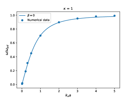
Figure 3: Analytical (line) and numerical (points) longitudinal dispersion relations plotted with screening parameter $\kappa$ = 1 and without rotation.

The present analysis is done using one-dimensional propagation of the wave, by choosing k = $k\hat{x}$ such that E = $E_{x}\hat{x}$ and the only the longitudinal perturbations are recovered. In order to analyze solution regime relevant to existing experiments incorporating dust rotation Hartmann et al. (2013), for the present computations we have used $\Omega$ $\approx$ 23.3 to 25 rad/s and $\omega_{\rm pd}$ $\approx$ 66 to 106 rad/s, which translates in the range of parameter $\beta$ $\approx$ 0.4 to 0.8. The rest of the parameters are also chosen to have their experimental value. Accordingly, $m_{\rm d}$ = 6.64$\times$ $10^{-14}$ kg, $q_{\rm d}$ = 6300$e$. Similarly the value of parameter $\kappa$ is also used as in the experiment for the corresponding cases. The computations are done for the three cases, obtaining the dispersion relation as plotted in figures presented further below in this section.

As the first, reference case, Fig. 3 shows the longitudinal wave dispersion relation in the absence of rotation ($\Omega$ = 0). This represents the dispersion relation for a regular dust acoustic wave in the laboratory frame with frequency saturating into the value $\omega=\omega_{\rm pd}$ for large $k$ values, or in the limit $ka\gg 1$. The dots in the Fig. 3 represent the simulated value, whereas the solid line is the analytic dispersion relation.

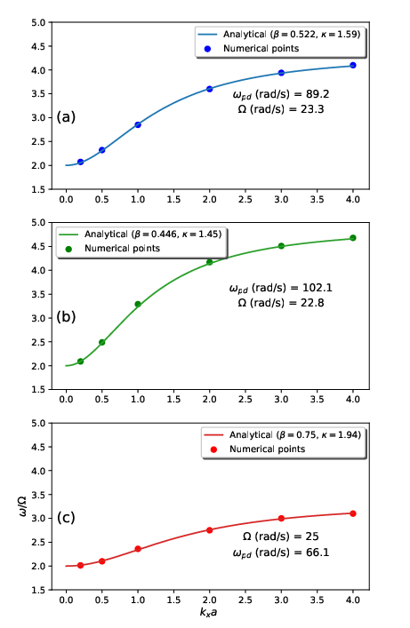
Figure 4: Analytical (lines) and numerical (points) longitudinal dispersion relations plotted with (a) $\Omega$ = 23.3 rad/s, $\omega_{pd}$ = 89.2 rad/s and $\kappa$ = 1.54, (b) $\Omega$ = 22.3 rad/s, $\omega_{pd}$ = 102.1 rad/s and $\kappa$ = 1.45, and (c) $\Omega$ = 25 rad/s, $\omega_{pd}$ = 66.3 rad/s and $\kappa$ = 1.94.

Results plotted in Fig. 4 show the longitudinal wave dispersion relation for a finite values of $\Omega$ and therefore they indeed correspond to transformed data from the laboratory measurements which are obtained in a rotating frame. The sets of parameters for producing the cases in Fig. 4 are derived from the experimental conditions of Ref. (Hartmann et al., 2013), where dispersion data was measured over a range of $\beta$ and $\kappa$ values in the frame of reference co rotating with the dust cloud. Similar to Fig. 3, the dots in the Fig. 4(a)-4(c) represent the simulated value, whereas the solid lines are the analytic dispersion relations, plotted here using the same set of parameters as used in the corresponding experimental cases. The frequency values on the entire $ka$ range for all the three cases presented in Fig. 4(a)-4(c) closely agree with the experimental measurements.

In more specific terms, the dispersion relation plot presented in Fig. 4(a) corresponds to the set of parameters, $\Omega$ = 23.3 rad/s, $\omega_{pd}$ = 89.2 rad/s (i.e.$\beta=0.522$) and $\kappa$ = 1.54. The dispersion at value $k\rightarrow 0$ is found to start duly from frequency 2$\Omega=46.6$ rad/s. At low wave numbers, the excitation frequency increases with the wave number which agree with the experimental results (Hartmann et al., 2013) and with increasing $k$-value, depending upon $\beta$, wave dispersion relation attains a saturated value which also confirms with what measured in the experiment. Similarly, the dispersion relation plotted in Fig. 4(b) is also simulated using the set of parameters, $\Omega$ = 22.3 rad/s, $\omega_{pd}$ = 102.1 rad/s (i.e., $\beta=0.466$) and $\kappa$ = 1.45, and shows the same trend when compared to experimental data. Note, however, that although all dispersion curves start with frequency which is two times the rotation frequency at ${k\rightarrow 0}$, their height, or the saturated value at ${k\gg 1}$ are different in each case, and increase in this saturated value is also in close agreement with the experimental observation for the corresponding. The last set plotted for comparison with experiments in Fig 4(c) corresponds to the set of parameters using stronger rotation, $\Omega$ = 25 rad/s, $\omega_{pd}$ = 66.3 rad/s (i.e., $\beta=0.75$) and $\kappa$ = 1.94. The saturation value of the frequency for this set is found to be minimum among the three cases presented. The dispersion curves therefore show a tendency to flatten and approach a minimum value as the value of parameter $\beta$ is increased. This limit is discussed further in the additional cases presented for a detailed analysis, independent of experiments, further below.

The overall agreement with the experimental observations is found better for the cases with higher $\beta=2\Omega/\omega_{\rm pd}$. For example, the saturation value of the present RPA results plotted for the third set of parameters in Fig. 4(c), as well as that in the corresponding experimental case, is $\omega/\Omega\sim 3$, which is in very close agreement with each other. This difference between the two however grows for smaller $\Omega$, i.e., in the cases plotted in Fig. 4(a) and 4(b) where the RPA results saturate at slightly higher values than the corresponding experimental levels. As an additional aspect, the saturation in the $\omega({\bf k})$ is attained when full 3-dimensional form of the potential, $\psi_{dD}\equiv\phi_{3D}$ is accounted for. While using the exact 2-dimensional form for $\psi_{dD}$ does not produce saturation in $\omega({\bf k})$ Jiang et al. (2007), the 3-dimensional form applies when the axial (along $\hat{z}$) variation in the dust cloud is rather week because of boundaries in $\hat{z}$ direction are sufficiently distant creating a nearly 3-dimensional dust cloud. The above agreement therefore additionally highlights enhanced 3-dimensional attributes of the dust dynamics in a rotating dust experiment, and, in turn, a subdued impact of the sedimentation usually produced by gravity in typical laboratory dusty plasmas that are levitated by an upward directed sheath potential of a horizontally placed electrode.

III.3 Longitudinal-Transverse coupling by dust rotation

The two dimensional numerical simulations on an extended 2-D grid allows us to illustrate the inevitable coupling between the longitudinal and transverse excitations and emergence of compression in an initially pure transverse shear like (non-compressional) perturbation of the 2-D velocity field. This effect readily follows from the solution (28) which is reducible in two independent longitudinal and transverse dispersion relations, (31) and (32), only in the limit $\Omega\rightarrow 0$.

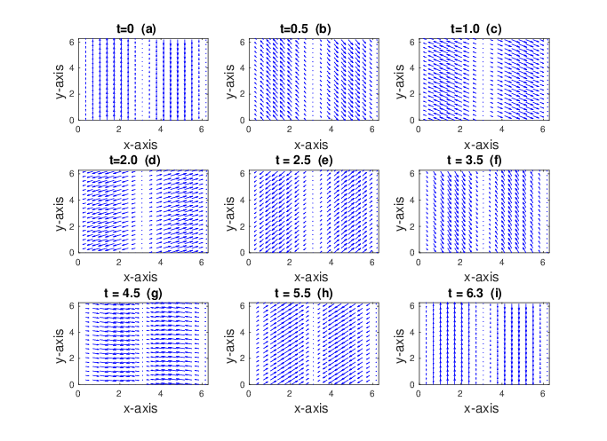
Figure 5: 2D velocity vector field profiles at different time for $\kappa\rightarrow\infty$ and $\beta=1$ ($\Omega=\omega_{\rm pd}/2)$, i.e., the velocity vector complets one rotation in half the system rotation.

Illustrating this coupling between the two modes in a rotating dust setup, the total velocity vector field is plotted in Fig. 5 at different phases (subperiodic time values) of an initially divergence free velocity perturbation as visible in Fig. 5(a). The evolution is presented for $\kappa\rightarrow\infty$ and $\Omega>0$ case when no electric field is expected because of perfectly shielded dust. The periodic evolution of the velocity field through Fig. 5(a)-Fig. 5(i) displayes emergence of divergent fields at the intermediate phases (e.g., t=2.0, 4.5 $\omega_{\rm pd}^{-1}$). Consequently, in the general case of an imperfectly shielded dust, finite electrostatic field would still develop, even if the initial perturbations are chosen to be purely divergence-free, ruling out a pure shear wave.

III.4 General characterization with respect to $\beta$ and $\kappa$

Independent of their comparison with experimental data sets, a more systematic additional analysis is presented in Fig. 6 and Fig. 7 which are obtained by simulating the cases with exclusive variation in the parameters $\beta$ and $\kappa$, respectively.

The value of $\beta=0.4$, 0.6 and 0.8 are used for the dispersion relations presented in Fig. 7(a) with a fixed value of $\kappa=1.41$. The increase in strength of rotation or $\beta$ reduces the rise of wave frequency value from the rotational frequency $\Omega$ and also the saturated value of the wave frequency. This tendency indicates the dominance of the Coriolis force effect over the electrostatic force effects, associated with dust acoustic mode, in the original equation of motion (1) written in the rotating frame. In order to highlight the behavior of the dispersion curve in the limiting case of very high rotation, dispersion curve is presented for a very high $\beta$ value (dashed line) showing that the wave frequency can be almost independent of $k$ and nearly equal to $2\Omega$ for very large $\beta$.

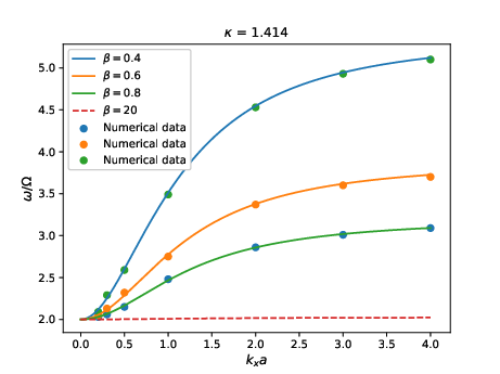
Figure 6: Analytical (lines) and numerical (points) longitudinal wave dispersion relations plotted with different value of $\beta$ and constant $\kappa$ = 1.41.

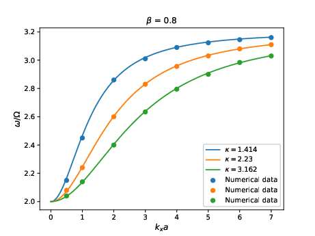
Figure 7: Analytical (lines) and numerical (points) longitudinal wave dispersion relations plotted with different value of $\kappa$ and constant $\beta$ = 0.8 .

The impact of screening parameter $\kappa=a/\lambda_{\rm D}$ on the mode frequency is similarly analyzed in Fig. 7(b) where dispersion curve with values of $\kappa=1.41$, 2.23 and 3.16 and a fixed value of $\beta=0.8$, are plotted, respectively. Increase in $\kappa$ value, or high dust density, causes an early saturation of the dispersion curve with respect to $ka$. While the saturated value of the frequency remains independent of $\kappa$, at very small screening parameter the approach to the saturated value become very slow with increasing $ka$.

III.5 Approach to weak coupling like effects by rotation

While the QLCA expressions for frequencies apply to general cases, including the effects of strong coupling, the numerical solutions presented and compared with the experimental results are from the fluid model corresponding to the random phase approximation (RPA) limit of the QLCA formulation. The observed close correspondence between this the weakly coupled regime of the model to somewhat contrasting considerations of strongly coupled limit of the dust particles as understood in the rotating plasma experiment (Hartmann et al., 2013) motivates us to explore the possible explanations. Especially as the correspondence is seen to improve between the two for higher rotation frequency, as discussed further below. Two aspects can be discussed in this respect reconciling the agreement of the experimental data with the weak coupling (RPA) results rather than with the branches corresponding to the strong coupling for which $D_{\mu\nu}$ remains finite. The first argument uses the non-equilibrium thermodynamic state of dust medium which is driven externally by an applied rotation. Considering that the dust medium is not in its thermal equilibrium, perhaps a modification in its coupling strength description can be explored in order to accommodate the parameter other than temperature in quantifying its effective coupling. A nonequilibrium state is no longer described by a single state parameter. Since the equilibrium ensembles yield the dust temperature as the unique parameter describing its thermodynamic state, this remains the only variable determining the degree of coupling in the dust for non rotating conditions, or even a magnetized dusty plasma. Rotating dust, on the other hand, being an open system and therefore operating away from the thermodynamic equilibrium presents a case, distinct from both non-rotating as well as magnetized dusty plasma that are essentially in a thermodynamical equilibrium.

An alternate argument relates to admitting only a small variation in its thermodynamical state from the equilibrium state, but attributing it to a possible rise, introduced by the external rotation, in the internal energy of the dust medium that results in its effective transition to a well defined weakly coupled, or fluid-like, regime under the standard, equilibrium formulation. This argument is also supported by the clearly measured changes in the characteristic parameters of the dust when rotation is switched on. For example, shown using a four particle dust cluster by Kählert et al.(Kählert et al., 2012) that as compared to the non-rotating case, the system is closer to the liquid state and has a lower Coulomb coupling. In a harmonic potential with confinement frequency $\omega_{\perp}$, the coupling parameter in rotating and non-rotating configurations, scale as $\Gamma(\Omega)/\Gamma(0)=(1-\Omega^{2}/\omega_{\perp}^{2})^{1/3}$, while the screening parameter scales as, $\kappa(\Omega)/\kappa(0)=(1-\Omega^{2}/\omega_{\perp}^{2})^{-1/3}$. We indeed note that the agreement with the experimental observations is improved significantly for the cases with higher $\beta=2\Omega/\omega_{\rm pd}$. For example, the saturation value of the present RPA results plotted for the third set of parameters in Fig. 4(c), as well as that in the corresponding experimental case, is $\omega/\Omega\sim 3$, which are therefore in very close agreement with each other. This agreement however becomes slightly poorer at weaker rotation frequency $\Omega$, or for small $\beta$ as in the cases plotted in Fig. 4(a) and 4(b) where the RPA results predict saturation at slightly higher values than the experiment. It should be further noted that in the present formulation treating a stably rotating dust fluid, the confining frequency $\omega_{\perp}$ is considered to be suitably high such that rotations with large enough $\Omega$ are admissible and $\Gamma$ and $\kappa$ are nearly independent of $\Omega/\omega_{\perp}$ Kählert et al. (2012). In contrast, the change in experimental dust parameters with respect to $\Omega$ is much stronger for the weak coupling effect to be more clearly visible at larger $\Omega$.

Both these scenarios however highlight a distinction between the underlying thermodynamical characters of a dusty plasma which is subjected to a magnetic field and the one which is subjected to an externally enforced rotation. The latter transforming its thermodynamical state to an open system, therefore no longer being governed by an equilibrium formulation.

IV Summary and conclusion

In the treatment presented we worked out a QCLA formulation which explicitly accounts for dust rotation in a Yukawa system. Its limiting case is derived corresponding to the weakly coupled (or RPA) limit where it yields equivalence to the regular explicitly rotating “dust fluid” formulation. Finite rotation version of both strong and weak coupling case dispersion relation is derived and analyzed, showing correspondence between ‘the faster rotating but weakly coupled’ and the strongly coupled dust responses. By presenting an equivalent multi-fluid rotating dusty plasma model and by means of its computational solutions for the parameters as in recent rotating dusty plasma experiments, independent agreement with analytical RPA dispersion relations is produced. A systematic characterization of the solutions with respect to variation in rotation frequency $\omega$ and screening parameter $\kappa$ is done separately. The analytical and numerical analysis of the rotating plasma dispersion showed that if the weakly coupled limit is considered with distant axial boundaries (3D effects), the frequency saturation not only becomes achievable in the rotating dusty plasma but the saturated frequency values also show quantitative agreement with those recovered in the recent experiments of the rotating dusty plasmas. This behavior indicates that a dust medium with large enough coupling parameter $\Gamma$, when driven to a nonequilibrium state by an external rotation, not only displays weak coupling like effects but also a relaxation from the boundary effects such that the plasma bulk strongly limited by axial boundaries still displays nearly 3D characteristics. The rotation of the dust thus additionally appears to relax the 2D effects (2D sedimentation, usually generated by the gravity) on the dust cloud. It is therefore concluded that this nonequilibrium rotating system not only shows isomorphism with magnetized dust regime but perhaps also with its microgravity regime, rendering the latter realizable also in the regular ground based laboratory experiments, if dust is subjected to a rotation. The analysis therefore motivates studies both in magnetized as well as in microgravity conditions in order to examine their similarity with ground based rotating dusty plasma experiments. The analysis may thus serve as a link between ground based magnetized dusty plasma experiments, like MDPX, and the International Space Station (ISS) based experiments in microgravity conditions.

V AIP PUBLISHING DATA SHARING POLICY

The data that support the findings of this study are available from the corresponding author upon reasonable request.

References

- Yaroshenko et al. (2007) V. Yaroshenko, F. Verheest, and G. Morfill, Astronomy & Astrophysics 461, 385 (2007).
- Yaroshenko et al. (2009) V. Yaroshenko, S. Ratynskaia, J. Olson, N. Brenning, J.-E. Wahlund, M. Morooka, W. Kurth, D. Gurnett, and G. Morfill, Planetary and Space Science 57, 1807 (2009).
- Shukla et al. (2003) P. Shukla, P. Dwivedi, and L. Stenflo, New Journal of Physics 5, 22 (2003).
- Nekrasov (2009) A. Nekrasov, The Astrophysical Journal 695, 46 (2009).
- Chabrier et al. (2002) G. Chabrier, F. Douchin, and A. Potekhin, Journal of Physics: Condensed Matter 14, 9133 (2002).
- Koester and Schönberner (1986) D. Koester and D. Schönberner, Astronomy and Astrophysics 154, 125 (1986).
- Willitsch et al. (2008) S. Willitsch, M. T. Bell, A. D. Gingell, and T. P. Softley, Physical Chemistry Chemical Physics 10, 7200 (2008).
- Pramanik et al. (2002) J. Pramanik, G. Prasad, A. Sen, and P. Kaw, Physical review letters 88, 175001 (2002).
- Quinn and Goree (2000) R. Quinn and J. Goree, Physics of Plasmas 7, 3904 (2000).
- Ghosh (2007) P. Ghosh, Rotation and accretion powered pulsars, Vol. 7 (World Scientific, 2007).
- Hewish et al. (1968) A. Hewish, S. J. Bell, J. D. Pilkington, P. F. Scott, and R. A. Collins, in Pulsating Stars (Springer, 1968) pp. 5–9.
- Uchida et al. (2004) G. Uchida, U. Konopka, and G. Morfill, Physical review letters 93, 155002 (2004).
- Thomas et al. (2015) E. Thomas, U. Konopka, D. Artis, B. Lynch, S. Leblanc, S. Adams, R. Merlino, and M. Rosenberg, Journal of Plasma Physics 81 (2015).
- Thomas et al. (2012) E. Thomas, R. Merlino, and M. Rosenberg, Plasma Physics and Controlled Fusion 54, 124034 (2012).
- Kählert et al. (2012) H. Kählert, J. Carstensen, M. Bonitz, H. Löwen, F. Greiner, and A. Piel, Physical review letters 109, 155003 (2012).
- Hartmann et al. (2013) P. Hartmann, Z. Donkó, T. Ott, H. Kählert, and M. Bonitz, Physical Review Letters 111, 155002 (2013).
- kaur et al. (2015) M. kaur, S. Bose, P. Chattopadhyay, D. Sharma, J. Ghosh, Y. C. Saxena, and E. J. Thomas, Physics of Plasmas 22, 093702 (2015).
- Kumar and Sharma (2020) P. Kumar and D. Sharma, Physics of Plasmas 27, 063703 (2020).
- Golden and Kalman (2000) K. I. Golden and G. J. Kalman, Physics of Plasmas 7, 14 (2000).
- Kalman and Golden (1990) G. Kalman and K. Golden, Physical Review A 41, 5516 (1990).
- Golden et al. (1992) K. I. Golden, G. Kalman, and P. Wyns, Physical Review A 46, 3454 (1992).
- Hou et al. (2009) L.-J. Hou, Z. Mišković, A. Piel, and M. S. Murillo, Physical Review E 79, 046412 (2009).
- Jiang et al. (2007) K. Jiang, Y.-H. Song, and Y.-N. Wang, Physics of Plasmas 14, 103708 (2007).
- Khrapak et al. (2016a) A. Khrapak, V. Molotkov, A. Lipaev, D. Zhukhovitskii, V. Naumkin, V. Fortov, O. Petrov, H. Thomas, S. Khrapak, P. Huber, et al., “Complex plasma research under microgravity conditions: Pk-3 plus laboratory on the international space station,” (2016a).
- Pustylnik et al. (2016) M. Pustylnik, M. Fink, V. Nosenko, T. Antonova, T. Hagl, H. Thomas, A. Zobnin, A. Lipaev, A. Usachev, V. Molotkov, et al., Review of scientific instruments 87, 093505 (2016).
- Fortov et al. (2003) V. Fortov, O. Vaulina, O. Petrov, V. Molotkov, A. Chernyshev, A. Lipaev, G. Morfill, H. Thomas, H. Rotermell, S. Khrapak, et al., Journal of Experimental and Theoretical Physics 96, 704 (2003).
- Golden et al. (1993) K. I. Golden, G. Kalman, and P. Wyns, Physical Review B 48, 8882 (1993).
- Khrapak et al. (2016b) S. A. Khrapak, B. Klumov, L. Couedel, and H. M. Thomas, Physics of Plasmas 23, 023702 (2016b).
- Khrapak (2017) S. A. Khrapak, AIP Advances 7, 125026 (2017).
- Khrapak et al. (2019) S. A. Khrapak, A. G. Khrapak, N. P. Kryuchkov, and S. O. Yurchenko, The Journal of chemical physics 150, 104503 (2019).