Stability and convergence of Strang splitting. Part I: Scalar Allen-Cahn equation

Abstract.

We consider a class of second-order Strang splitting methods for Allen-Cahn equations with polynomial or logarithmic nonlinearities. For the polynomial case both the linear and the nonlinear propagators are computed explicitly. We show that this type of Strang splitting scheme is unconditionally stable regardless of the time step. Moreover we establish strict energy dissipation for a judiciously modified energy which coincides with the classical energy up to $\mathcal{O}(\tau)$ where $\tau$ is the time step. For the logarithmic potential case, since the continuous-time nonlinear propagator no longer enjoys explicit analytic treatments, we employ a second order in time two-stage implicit Runge–Kutta (RK) nonlinear propagator together with an efficient Newton iterative solver. We prove a maximum principle which ensures phase separation and establish energy dissipation law under mild restrictions on the time step. These appear to be the first rigorous results on the energy dissipation of Strang-type splitting methods for Allen-Cahn equations.

1. Introduction

In this work we consider the Allen-Cahn equation [1] of the form

$$\begin{cases}\partial_{t}u=\varepsilon^{2}\Delta u-f(u),\qquad(t,x)\in(0,\infty)\times\Omega;\\ u\Bigr{|}_{t=0}=u^{0},\end{cases}$$ (1.1)

where $u$ is a real-valued function corresponding to the concentration of a phase in a multi-component alloy, and $u^{0}$ is the initial condition. For simplicity we take the spatial domain $\Omega$ to be the $2\pi$-periodic torus $\mathbb{T}^{d}=[-\pi,\pi]^{d}$ in physical dimensions $d\leq 3$. With some minor work our analysis can be extended to many other situations. The parameter $\varepsilon^{2}>0$ is the mobility coefficient which is fixed as a constant. In its present non-dimensionalized form the magnitude of $\varepsilon$ governs the typical length scale of an interface in the dynamical evolution. The nonlinear term $f(u)$ is taken as the derivative of a given potential function, namely $f(u)=F^{\prime}(u)$. We will be primarily concerned with two typical potential functions. One is the standard double-well potential

$$F_{\mathrm{st}}(u)=\frac{1}{4}(u^{2}-1)^{2}$$ (1.2)

whose extrema $u=\pm 1$ correspond to two different phases. The other is the logarithmic Flory–Huggins free energy [2, 3]

$$F_{\mathrm{fh}}(u)=\frac{\theta}{2}[(1+u)\ln(1+u)+(1-u)\ln(1-u)]-\frac{\theta_{c}}{2}u^{2},$$ (1.3)

where $0<\theta<\theta_{c}$ denote the absolute temperature and the critical temperature respectively. The condition $0<\theta<\theta_{c}$ is very physical since it ensures that $F_{\mathrm{fh}}$ has a double-well form with two equal minima situated at $u_{+}$ and $-u_{+}$, where $u_{+}>0$ is the positive root of the equation

$$0=F_{\mathrm{fh}}^{\prime}(u)=\frac{\theta}{2}\ln\frac{1+u}{1-u}-\theta_{c}u.$$ (1.4)

When the quenching is shallow (i.e. $\theta$ is close to $\theta_{c}$), one can Taylor-expand near $u=0$ and obtain the standard polynomial approximation of the free energy. For smooth solutions of (2.34), we have the energy dissipation

$$\frac{d}{dt}E(u)\leq 0,$$ (1.5)

where

$$E(u)=\int_{\Omega}\Bigl{(}\frac{\varepsilon^{2}}{2}|\nabla u|^{2}+F(u)\Bigr{)}dx,$$ (1.6)

and $F(u)=F_{\mathrm{st}}(u)$ or $F_{\mathrm{fh}}(u)$. In practical numerical simulations, the energy dissipation law is often used as a fidelity check of the algorithm.

In this work we shall analyze the stability of second-order in time splitting methods applied to the Allen-Cahn equation. Due to its simplicity the operator splitting methods have found its ubiquitous presence in the numerical simulation of many physical problems, including phase-field equations [4, 5, 15, 16, 17, 18], Schrödinger equations [6, 7, 20], and the reaction-diffusion systems [8, 9]. A prototypical second order in time method is the Strang splitting approximation [10, 11]. Specifically for the Allen–Cahn equation under study, we adopt the following Strang splitting discretization

$$u^{n+1}=\mathcal{S}_{\mathcal{L}}\left(\tau/2\right)\mathcal{S}_{\mathcal{N}}\left(\tau\right)\mathcal{S}_{\mathcal{L}}\left(\tau/2\right)u^{n},$$ (1.7)

where $\tau>0$ denotes the time step, and $S_{\mathcal{L}}(\frac{1}{2}\tau)=\exp(\varepsilon^{2}\frac{1}{2}\tau\Delta)$ is the linear propagator. The nonlinear propagator $S_{\mathcal{N}}(\tau):a\mapsto u(\tau)$ is the nonlinear solution operator of the system

$$\begin{cases}\partial_{t}u=-f(u),\\ u\Bigr{|}_{t=0}=a.\end{cases}$$ (1.8)

Denote by $S_{\mathrm{ex}}(\tau)$ the exact nonlinear solution operator to (2.34). The propagator (1.7) is a second order in time approximation in the sense that it admits

$$\text{$\mathcal{O}(\tau^{3})$ one-step approximation error}:\qquad S_{\mathrm{ex}}(\tau)u^{n}=u^{n+1}+\mathcal{O}(\tau^{3});$$ (1.9)

$$\text{$\mathcal{O}(\tau^{2})$ in-$\mathcal{O}(1)$-time approximation error}:\qquad\sup_{n\tau\leq T}\|u^{n}-S_{\mathrm{ex}}(n\tau)u^{0}\|=\mathcal{O}(\tau^{2}).$$ (1.10)

Here $[0,T]$ is a given compact time interval, $\|\cdot\|$ is some Sobolev norm and the implied constants in $\mathcal{O}(\tau^{2})$ can depend on $T$. As it turns out the numerical performance of the scheme (1.7) is quite good for solving the Allen-Cahn equation [5]. On the other hand, it should be noted that the somewhat heuristic estimates (1.9)–(1.10) rest on various subtle regularity assumptions on the exact solution and the numerical iterates. A fundamental open issue is to establish the stability and regularity of the Strang splitting solutions in various Sobolev classes. The very purpose of this paper is to settle this problem for the Allen-Cahn equation (2.34) with the polynomial or the logarithmic potential nonlinearities. Our first result is concerned with the polynomial case. Note that in this case the nonlinear propagator $S_{\mathcal{N}}(\tau)$ can be expressed explicitly.

Theorem 1.1 (Stability of Strang-splitting for AC, polynomial case).

Let $\varepsilon>0$, $d\leq 3$ and consider (2.34) on the periodic torus $\mathbb{T}^{d}=[-\pi,\pi]^{d}$ with $f(u)=u^{3}-u$. Let $\tau>0$ and denote $S_{\mathcal{L}}(\tau)=\exp(\varepsilon^{2}\tau\Delta)$. Denote $S_{\mathcal{N}}(\tau)$ according to (1.8). Consider the Strang splitting discretization

$$u^{n+1}=\mathcal{S}_{\mathcal{L}}\left(\tau/2\right)\mathcal{S}_{\mathcal{N}}\left(\tau\right)\mathcal{S}_{\mathcal{L}}\left(\tau/2\right)u^{n},\qquad n\geq 0.$$ (1.11)

The following hold.

1. The maximum principle. For any $\tau>0$ and any $n\geq 0$, it holds that

   $$\|u^{n+1}\|_{\infty}\leq\max\{1,\;\|u^{n}\|_{\infty}\}.$$ (1.12)

   It follows that

   $$\sup_{n\geq 1}\|u^{n}\|_{\infty}\leq\max\{1,\;\|u^{0}\|_{\infty}\}.$$ (1.13)

   In particular if $\|u^{0}\|_{\infty}\leq 1$, then

   $$\sup_{n\geq 1}\|u^{n}\|_{\infty}\leq 1.$$ (1.14)

2. Modified energy dissipation. Let $u^{0}\in H^{1}(\mathbb{T}^{d})$. For any $\tau>0$ and any $n\geq 0$, we have

   $$\widetilde{E}^{n+1}\leq\widetilde{E}^{n}.$$ (1.15)

   Here (below $\langle,\rangle$ denotes the usual $L^{2}$ inner product)

   $$\widetilde{E}^{n}=\frac{1}{2\tau}\langle(1-e^{\varepsilon^{2}\tau\Delta})u^{n},\,u^{n}\rangle+\int_{\mathbb{T}^{d}}\widetilde{F}(\tilde{u}^{n})dx$$ (1.16)

   $$\quad\;=\frac{1}{2\tau}\langle(e^{-\varepsilon^{2}\tau\Delta}-1)\tilde{u}^{n},\,\tilde{u}^{n}\rangle+\int_{\mathbb{T}^{d}}\widetilde{F}(\tilde{u}^{n})dx;$$ (1.17)

   $$\;\;\tilde{u}^{n}=\mathcal{S}_{\mathcal{L}}(\tau/2)u^{n};$$ (1.18)

   $$\;\;\widetilde{F}(\tilde{u}^{n})=\frac{1}{4}+\frac{1}{2\tau}(\tilde{u}^{n})^{2}-\frac{e^{\tau}}{\tau(e^{2\tau}-1)}\left(\sqrt{1+(e^{2\tau}-1)(\tilde{u}^{n})^{2}}-1\right).$$ (1.19)

3. Uniform Sobolev bounds. Let $u^{0}\in H^{k_{0}}(\mathbb{T}^{d})$ for some $k_{0}\geq 1$. It holds that

   $$\sup_{n\geq 1}\|u^{n}\|_{H^{k_{0}}(\mathbb{T}^{d})}\leq C_{1},$$ (1.20)

   where $C_{1}>0$ depends only on ($\varepsilon$, $k_{0}$, $d$, $\|u^{0}\|_{H^{k_{0}}}$). Moreover for any $k\geq k_{0}$, we have

   $$\sup_{n\geq\frac{1}{\tau}}\|u^{n}\|_{H^{k}(\mathbb{T}^{d})}\leq C_{2},$$ (1.21)

   where $C_{2}>0$ depends only on ($\varepsilon$, $k$, $k_{0}$, $d$, $\|u^{0}\|_{H^{k_{0}}}$ ).

4. Connection with the standard energy. Let $u^{0}$ be smooth (for example $u^{0}\in H^{20}(\mathbb{T}^{d})$). For $0<\tau\leq 1$, we have

   $$\sup_{n\geq 0}|\widetilde{E}^{n}-E(u^{n})|\leq C_{3}\tau,$$ (1.22)

   where $C_{3}>0$ depends only on ($\varepsilon$, $d$, $u^{0}$).

5. Uniform second order approximation. Assume the initial data $u^{0}$ is sufficiently smooth (for example $u^{0}\in H^{40}(\mathbb{T}^{d})$). Let $u$ be the exact PDE solution to (2.34) corresponding to initial data $u^{0}$. Let $0<\tau\leq 1$. Then for any $T>0$, we have

   $$\sup_{n\geq 1,n\tau\leq T}\|u^{n}-u(n\tau,\cdot)\|_{L^{2}(\mathbb{T}^{d})}\leq C\cdot\tau^{2},$$ (1.23)

   where $C>0$ depends on ($\varepsilon$, $u^{0}$, $T$).

Remark 1.1.

Consider the function

$$h(x)=\frac{1}{4}+\frac{1}{2\tau}x-\frac{e^{\tau}}{\tau(e^{2\tau}-1)}\left(\sqrt{1+(e^{2\tau}-1)x}-1\right),\;x\in[0,\infty).$$ (1.24)

Clearly, $h(0)=\frac{1}{4}$, $h(x)\rightarrow\infty$ as $x\rightarrow\infty$, and

$$h^{\prime}(x)=0\Leftrightarrow x=1.$$ (1.25)

We have

$$h(1) =\frac{1}{4}+\frac{1}{2\tau}-\frac{e^{\tau}}{\tau(e^{\tau}+1)}$$ (1.26)

$$=\frac{1}{4}-\frac{1}{2\tau}\frac{e^{\tau}-1}{e^{\tau}+1}\geq 0,\quad\forall\,0\leq\tau<\infty.$$ (1.27)

Thus $\widetilde{F}$ defined in (1.19) is always nonnegative. On the other hand, by using Fourier transform, we have

$$\langle(e^{-\varepsilon^{2}\tau\Delta}-1)w,\,w\rangle=c_{d}\sum_{0\neq k\in\mathbb{Z}^{d}}(e^{\varepsilon^{2}\tau|k|^{2}}-1)|\widehat{w}(k)|^{2}\geq 0,$$ (1.28)

where $c_{d}>0$ depends only on the dimension $d$. Therefore $\widetilde{E}$ always stays nonnegative.

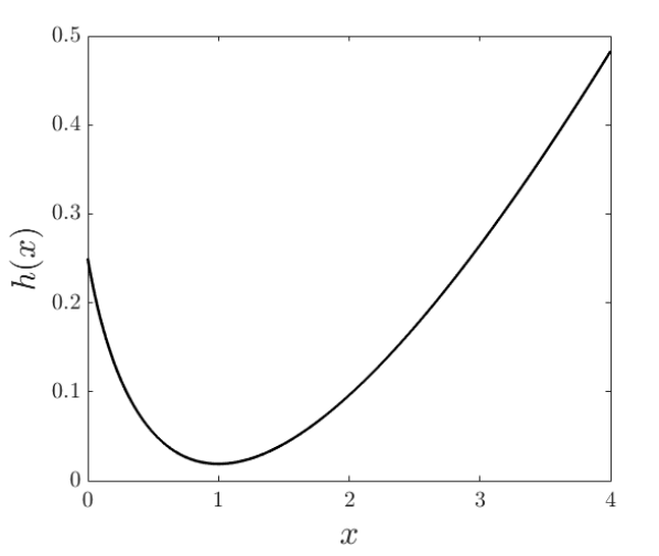
Figure 1. $h(x)$ w.r.t. $x$ for $\tau=1$.

Remark 1.2.

The regularity assumptions in (1.22) and (1.23) can be lowered. However for simplicity of presentation we do not dwell on this issue in this work.

Our second result focuses on the AC equation with the logarithmic potential (1.3), i.e.

$$\begin{cases}\partial_{t}u=\varepsilon^{2}\Delta u-f^{\mathrm{LOG}}(u),\qquad f^{\mathrm{LOG}}(u)=-\theta_{c}u+\frac{\theta}{2}\ln\frac{1+u}{1-u};\\ u\Bigr{|}_{t=0}=u^{0},\end{cases}$$ (1.29)

where $0<\theta<\theta_{c}$. It is not difficult to check that (cf. the analysis after (3.7)) $f^{\mathrm{LOG}}(u)$ admits a unique root in the interval $(0,1$) which we denote as $u_{*}$. For smooth solutions to (1.29), we have the maximum principle: $\|u(t,\cdot)\|_{\infty}\leq u_{*}$ for all $t>0$ if $\|u_{0}\|_{\infty}\leq u_{*}$. On the other hand, it is a nontrivial task to design suitable numerical discretization preserving this important maximum principle.

By direct analogy with the polynomial potential case, one can consider the exact Strang-type second order in time splitting scheme:

$$u^{n+1}=\mathcal{S}_{\mathcal{L}}(\tau/2)\mathcal{S}_{\mathcal{N}}^{(\mathrm{LOG})}(\tau)\mathcal{S}_{\mathcal{L}}(\tau/2)u^{n},$$ (1.30)

where $\mathcal{S}_{\mathcal{L}}(\tau)=\exp(\varepsilon^{2}\tau\Delta)$ and $\mathcal{S}_{\mathcal{N}}^{(\mathrm{LOG})}(\tau)$ is the solution operator $w_{0}\to w(\tau)$ of the equation

$$\begin{cases}\partial_{t}w=\theta_{c}w-\frac{\theta}{2}\ln\frac{1+w}{1-w},\quad 0<t\leq\tau;\\ w\Bigr{|}_{t=0}=w_{0}.\end{cases}$$ (1.31)

However a pronounced difficulty with the implementation of the above scheme is the lack of an explicit solution formula for the solver $\mathcal{S}_{\mathcal{N}}^{(\mathrm{LOG})}(\tau)$. To solve this problem we approximate $\mathcal{S}_{\mathcal{N}}^{(\mathrm{LOG})}(\tau)$ by a further judiciously chosen numerical discretization. The choice of the numerical solver turns out to be rather subtle and technically involved, since one has to control the truncation error to be within $\mathcal{O}(\tau^{3})$ and preserve the maximum principle at the same time (see the recent deep work of Li, Yang, and Zhou [14] where an ingenious cut-off procedure is developed).

To approximate $\mathcal{S}_{\mathcal{N}}^{(\mathrm{LOG})}(\tau)v$ for given $v$, we adopt the Pareschi and Russo’s two-stage diagonally implicit Runge Kutta (PR-RK) method [13]:

$$u_{1}=v+a\tau f(u_{1}),$$ (1.32)

$$u_{2}=v+(1-2a)\tau f(u_{1})+a\tau f(u_{2}),$$

$$\mathcal{S}_{\mathcal{N}}^{(\mathrm{LOG})}(\tau)v\approx\widetilde{\mathcal{S}}_{\mathcal{N}}(\tau)v:=v+\frac{1}{2}\tau f(u_{1})+\frac{1}{2}\tau f(u_{2}).$$

In the above $a$ is a tunable real-valued parameter.

We employ the following RK-based Strang-type splitting for (1.29):

$$u^{n+1}=\mathcal{S}_{\mathcal{L}}(\tau/2)\widetilde{\mathcal{S}}_{\mathcal{N}}(\tau)\mathcal{S}_{\mathcal{L}}(\tau/2)u^{n}.$$ (1.33)

In terms of $\tilde{u}^{n}=\mathcal{S}_{\mathcal{L}}(\tau/2)u^{n}$, we have:

$$\tilde{u}^{n+1}=\mathcal{S}_{\mathcal{L}}(\tau)\widetilde{\mathcal{S}}_{\mathcal{N}}(\tau)\tilde{u}^{n}.$$ (1.34)

We have the following stability result concerning the logarithmic case.

Theorem 1.2 (Stability of RK-based Strang-splitting for AC, logarithmic case).

Let $\varepsilon>0$, $d\leq 3$, $0<\theta<\theta_{c}$ and consider (1.29) on the periodic torus $\mathbb{T}^{d}=[-\pi,\pi]^{d}$. Recall $u_{*}$ is the unique root of $f^{\mathrm{LOG}}(u)$ in the interval $(0,1$). Let $\tau>0$ and consider the RK-based Strang-splitting scheme defined in (1.33) and equivalently expressed in terms of $\tilde{u}^{n}$ in (1.34). Assume $u^{0}\in H^{1}(\mathbb{T}^{d})$ and $\|u^{0}\|_{\infty}\leq u_{*}$. Assume $a\geq 1+\frac{\sqrt{2}}{2}$ and $0<\tau\leq\frac{1}{3a(\theta_{c}-\theta)}$. The following hold.

1. The maximum principle. It holds that

   $$\sup_{n\geq 1}\max\{\|u^{n}\|_{\infty},\;\|\tilde{u}^{n}\|_{\infty}\}\leq u_{*}<1.$$ (1.35)

2. Modified energy dissipation. We have

   $$\sup_{n\geq 1}\max\{\|u^{n}\|_{\infty},\;\|\tilde{u}^{n}\|_{\infty}\}\leq u_{*};$$ (1.36)

   $$\overline{E}^{n+1}\leq\overline{E}^{n},\quad\forall\;n\geq 1;$$ (1.37)

   $$\overline{E}^{n}\coloneqq\frac{1}{2}\left\langle\frac{1}{\tau}(e^{-\varepsilon^{2}\tau\Delta}-1)\tilde{u}^{n},\tilde{u}^{n}\right\rangle+\int_{\mathbb{T}^{d}}\overline{F}(\tilde{u}^{n})dx,$$ (1.38)

   where $\overline{F}$ is defined by (3.37).

3. Uniform Sobolev bounds. Let $u^{0}\in H^{k_{0}}(\mathbb{T}^{d})$ for some $k_{0}\geq 1$. It holds that

   $$\sup_{n\geq 1}\|u^{n}\|_{H^{k_{0}}(\mathbb{T}^{d})}\leq B_{1},$$ (1.39)

   where $B_{1}>0$ depends only on ($\varepsilon$, $k_{0}$, $d$, $\|u^{0}\|_{H^{k_{0}}}$, $\theta$, $\theta_{c}$). Moreover for any $k\geq k_{0}$, we have

   $$\sup_{n\geq\frac{1}{\tau}}\|u^{n}\|_{H^{k}(\mathbb{T}^{d})}\leq B_{2},$$ (1.40)

   where $B_{2}>0$ depends only on ($\varepsilon$, $k$, $k_{0}$, $d$, $\|u^{0}\|_{H^{k_{0}}}$, $\theta$, $\theta_{c}$ ).

4. Connection with the standard energy. Let $u^{0}$ be smooth (for example $u^{0}\in H^{20}(\mathbb{T}^{d})$). For $0<\tau\leq 1$, we have

   $$\sup_{n\geq 0}|\overline{E}^{n}-E(u^{n})|\leq B_{3}\tau,$$ (1.41)

   where $B_{3}>0$ depends only on ($\varepsilon$, $d$, $u^{0}$, $\theta$, $\theta_{c}$).

5. Uniform second order approximation. Assume the initial data $u^{0}$ is sufficiently smooth (for example $u^{0}\in H^{40}(\mathbb{T}^{d})$). Let $u$ be the exact PDE solution to (1.29) corresponding to initial data $u^{0}$. Let $0<\tau\leq 1$. For any $T>0$, we have

   $$\sup_{n\geq 1,n\tau\leq T}\|u^{n}-u(n\tau,\cdot)\|_{L^{2}(\mathbb{T}^{d})}\leq\widetilde{C}\cdot\tau^{2},$$ (1.42)

   where $\widetilde{C}>0$ depends on ($\varepsilon$, $u^{0}$, $T$, $\theta$, $\theta_{c}$).

Remark 1.3.

More generally, one can also show that if $\|u^{0}\|_{\infty}\leq\beta<1$ for some $\beta\in[u_{*},1)$, then $\|u^{n}\|_{\infty}\leq\beta$ for all $n\geq 1$. This slightly more maximum principle covers most common cases in practical simulations. In many cases $u_{*}$ is already close to the limit value $1$. For example if $\theta=\frac{1}{4}$, $\theta_{c}=1$ and $\varepsilon=0.01$, then $u_{*}\approx 0.99933$ which already serves as a good upper bound from a practical point of view.

The statement (3)–(5) in Theorem 1.2 can be proved in a similar way as in the polynomial case and we omit the repetitive details. The rest of this paper is organized as follows. In Section 2, we give the proof of Theorem 1.1. Section 3 is devoted to the proof of Theorem 1.2. As mentioned above we focus on proving statement (1)–(2) in Theorem 1.2. We give detailed exposition and motivation for these results therein. In Section 4, we carry out extensive numerical simulations to showcase the stability and convergence of the Strang-splitting methods for both the polynomial and the logarithmic cases. The last section contains some concluding remarks.

2. Proof of Theorem 1.1

In this section we carry out the proof of Theorem 1.1. We divide the proof into several steps.

2.1. The maximum principle

Recall that $u^{n+1}=\mathcal{S}_{\mathcal{L}}\left(\tau/2\right)\mathcal{S}_{\mathcal{N}}\left(\tau\right)\mathcal{S}_{\mathcal{L}}\left(\tau/2\right)u^{n}$. Since $\|S_{\mathcal{L}}(\tau)a\|_{\infty}\leq\|a\|_{\infty}$ for any $\tau>0$, we only need to examine $S_{\mathcal{N}}(\tau)$. By definition, the nonlinear solver is

$$\begin{cases}\partial_{t}u=u-u^{3},\quad 0<t\leq\tau;\\ u\Bigr{|}_{t=0}=a.\end{cases}$$ (2.1)

Thanks to the explicit polynomial nonlinearity, one can solve the above equation explicitly and obtain

$$u(t)=\frac{e^{t}a}{\sqrt{1+(e^{2t}-1)a^{2}}}.$$ (2.2)

This renders the solution operator $S_{\mathcal{N}}(\tau)$ as

$$\mathcal{S}_{\mathcal{N}}(\tau)a=\frac{e^{\tau}a}{\sqrt{1+(e^{2\tau}-1)a^{2}}}.$$ (2.3)

By (2.3), we have

$$\|\mathcal{S}_{\mathcal{N}}(\tau)a\|_{\infty}\leq\max\{\|a\|_{\infty},1\}.$$ (2.4)

This yields the desired maximum principle. Note that one can also work directly with (2.1) to derive (2.4).

2.2. Modified energy dissipation

Since $u^{n+1}=\mathcal{S}_{\mathcal{L}}\left(\tau/2\right)\mathcal{S}_{\mathcal{N}}\left(\tau\right)\mathcal{S}_{\mathcal{L}}\left(\tau/2\right)u^{n}$ and $\tilde{u}^{n}=\mathcal{S}_{\mathcal{L}}\left(\tau/2\right)u^{n}$, we have

$$\tilde{u}^{n+1}=\mathcal{S}_{\mathcal{L}}\left(\tau\right)\mathcal{S}_{\mathcal{N}}\left(\tau\right)\tilde{u}^{n}.$$ (2.5)

This yields

$$e^{-\varepsilon^{2}\tau\Delta}\tilde{u}^{n+1}=\frac{e^{\tau}\tilde{u}^{n}}{\sqrt{1+(e^{2\tau}-1)(\tilde{u}^{n})^{2}}}.$$ (2.6)

We rewrite the above as

$$\frac{1}{\tau}\left(e^{-\varepsilon^{2}\tau\Delta}-1\right)\tilde{u}^{n+1}+\frac{1}{\tau}(\tilde{u}^{n+1}-\tilde{u}^{n})=\frac{1}{\tau}\left(\frac{e^{\tau}\tilde{u}^{n}}{\sqrt{1+(e^{2\tau}-1)(\tilde{u}^{n})^{2}}}-\tilde{u}^{n}\right)=-\widetilde{F}^{\prime}(\tilde{u}^{n}),$$ (2.7)

where

$$\widetilde{F}(z)=\frac{1}{4}+\frac{1}{2\tau}z^{2}-\frac{e^{\tau}}{\tau(e^{2\tau}-1)}\left(\sqrt{1+(e^{2\tau}-1)z^{2}}-1\right).$$ (2.8)

The harmless constant $1/4$ is inserted here so that $\widetilde{F}$ coincides with the standard energy when $\tau\to 0$. Observe that

$$\tilde{F}(\tilde{u}^{n+1})=\tilde{F}(\tilde{u}^{n})+\tilde{F}^{\prime}(\tilde{u}^{n})(\tilde{u}^{n+1}-\tilde{u}^{n})+\frac{1}{2}\tilde{F}^{\prime\prime}(\xi^{n})(\tilde{u}^{n+1}-\tilde{u}^{n})^{2},$$ (2.9)

where $\xi^{n}$ is some function between $\tilde{u}^{n}$ and $\tilde{u}^{n+1}$. Also

$$\frac{1}{\tau}\langle(e^{-\varepsilon^{2}\tau\Delta}-1)\tilde{u}^{n+1},\tilde{u}^{n+1}-\tilde{u}^{n}\rangle$$

$$= \frac{1}{\tau}\langle(1-e^{\varepsilon^{2}\tau\Delta})u^{n+1},\,u^{n+1}-u^{n}\rangle$$

$$= \frac{1}{2\tau}\Bigl{(}\langle(1-e^{\varepsilon^{2}\tau\Delta})u^{n+1},u^{n+1}\rangle-\langle(1-e^{\varepsilon^{2}\tau\Delta})u^{n},u^{n}\rangle+\langle(1-e^{\varepsilon^{2}\tau\Delta})(u^{n+1}-u^{n}),u^{n+1}-u^{n}\rangle\Bigr{)}.$$ (2.10)

Multiplying (2.7) by $(\tilde{u}^{n+1}-\tilde{u}^{n})$, integrating over $\mathbb{T}^{d}$ and using (2.9)–(2.10), we obtain

$$\widetilde{E}^{n+1}-\widetilde{E}^{n}$$ (2.11)

$$=-\frac{1}{2\tau}\left\langle\left(1-e^{\varepsilon^{2}\tau\Delta}\right)(u^{n+1}-u^{n}),(u^{n+1}-u^{n})\right\rangle-\left\langle\left(\frac{1}{\tau}-\frac{1}{2}\widetilde{F}^{\prime\prime}(\xi^{n})\right)(\tilde{u}^{n+1}-\tilde{u}^{n})^{2},1\right\rangle.$$

It is not difficult to check that

$$\widetilde{F}^{\prime\prime}(\xi)=\frac{1}{\tau}-\frac{e^{\tau}}{\tau\left(1+(e^{2\tau}-1)\xi^{2}\right)^{\frac{3}{2}}}.$$ (2.12)

Clearly

$$\frac{1}{\tau}-\frac{1}{2}F^{\prime\prime}(\xi)\geq 0,\qquad\forall\,\xi\in\mathbb{R}.$$ (2.13)

Thus we have $\widetilde{E}^{n+1}\leq\widetilde{E}^{n}$ for all $n\geq 0$.

2.3. Uniform Sobolev bounds

To establish uniform Sobolev bounds on $u^{n}$, we first show that it suffices to prove

$$\sup_{n\geq 1}\|\tilde{u}^{n}\|_{H^{k_{0}}}\leq D_{1},$$ (2.14)

where $D_{1}>0$ depends only on ($\varepsilon$, $k_{0}$, $\|u^{0}\|_{H^{k_{0}}}$, $d$).

Indeed assume (2.14) holds, we now check the uniform bound on $u^{n+1}$. For simplicity we conduct the argument for $k_{0}=1$, i.e. we check the $H^{1}$ bound. The general $k_{0}\geq 2$ case is similar and omitted (see e.g. the bootstrap argument developed in [19, Section 2.7.2]). Since $u^{n+1}=\mathcal{S}_{\mathcal{L}}\left(\tau/2\right)\mathcal{S}_{\mathcal{N}}\left(\tau\right)\mathcal{S}_{\mathcal{L}}\left(\tau/2\right)u^{n}$ and $\tilde{u}^{n}=\mathcal{S}_{\mathcal{L}}\left(\tau/2\right)u^{n}$, we have

$$u^{n+1}=\mathcal{S}_{\mathcal{L}}\left(\tau/2\right)\mathcal{S}_{\mathcal{N}}(\tau)\tilde{u}^{n}.$$ (2.15)

By examining the structure of the equation $\partial_{t}u=u-u^{3}$, it is not difficult to check that

$$\|\nabla(\mathcal{S}_{\mathcal{N}}(\tau)a)\|_{2}\leq e^{\tau}\|\nabla a\|_{2},$$ (2.16)

$$\|\mathcal{S}_{\mathcal{N}}(\tau)a\|_{2}\leq\max\{\|a\|_{2},\;C_{d}\},$$ (2.17)

where $C_{d}>0$ is a constant depending only on the dimension $d$. We then discuss two cases. If $0<\tau\leq 1$, we use (2.16)–(2.17) and obtain

$$\|u^{n+1}\|_{H^{1}}\leq\|\mathcal{S}_{\mathcal{N}}(\tau)\tilde{u}^{n}\|_{H^{1}}\leq D_{2},$$ (2.18)

where $D_{2}>0$ depends only on ($\varepsilon$, $\|u^{0}\|_{H^{1}}$, $d$). If $\tau>1$, we use (2.17) and obtain

$$\|u^{n+1}\|_{H^{1}}\lesssim\|\mathcal{S}_{\mathcal{N}}(\tau)\tilde{u}^{n}\|_{2}\leq D_{3},$$ (2.19)

where $D_{3}>0$ depends only on ($\varepsilon$, $\|u^{0}\|_{H^{1}}$, $d$). Thus in both cases we obtain the uniform bound on $u^{n+1}$.

We now focus on (2.14). For simplicity we assume $k_{0}=1$. The general case $k_{0}\geq 2$ follows along similar lines using smoothing estimates and we omit the details.

Consider first the case $0<\tau\leq 1$. We rewrite

$$\widetilde{F}(z) =\frac{1}{4}+\frac{1}{2\tau}z^{2}-\frac{e^{\tau}}{\tau}\cdot\frac{z^{2}}{1+\sqrt{1+(e^{2\tau}-1)z^{2}}}$$

$$=\frac{1}{4}+\frac{1}{2\tau}z^{2}-\frac{1}{\tau}\cdot\frac{z^{2}}{1+\sqrt{1+(e^{2\tau}-1)z^{2}}}-\frac{e^{\tau}-1}{\tau}\cdot\frac{z^{2}}{1+\sqrt{1+(e^{2\tau}-1)z^{2}}}$$

$$=\frac{1}{4}+\frac{e^{2\tau}-1}{2\tau}\cdot\frac{z^{4}}{\big{(}1+\sqrt{1+(e^{2\tau}-1)z^{2}}\big{)}^{2}}-\frac{e^{\tau}-1}{\tau}\cdot\frac{z^{2}}{1+\sqrt{1+(e^{2\tau}-1)z^{2}}}$$

$$=\frac{e^{2\tau}-1}{2\tau}\Bigl{(}\big{(}A-\frac{1}{1+e^{\tau}}\big{)}^{2}-\frac{1}{(1+e^{\tau})^{2}}\Bigr{)}+\frac{1}{4},$$ (2.20)

where $A=z^{2}/\big{(}1+\sqrt{1+(e^{2\tau}-1)z^{2}}\big{)}$.

Since $d\leq 3$, by using the above expression together with Sobolev embedding, we have

$$\int_{\mathbb{T}^{d}}\widetilde{F}(u^{0})dx\leq D_{4},$$ (2.21)

where $D_{4}>0$ depends only on ($\|u^{0}\|_{H^{1}(\mathbb{T}^{d})}$, $d$). It follows that uniformly in $n$,

$$\frac{1}{2}\varepsilon^{2}\|\nabla\tilde{u}^{n}\|_{2}^{2}\leq\frac{1}{2\tau}\langle(e^{-\varepsilon^{2}\tau\Delta}-1)\tilde{u}^{n},\,\tilde{u}^{n}\rangle\leq D_{5},$$ (2.22)

where $D_{5}>0$ depends only on ($\|u^{0}\|_{H^{1}(\mathbb{T}^{d})}$, $d$, $\varepsilon$). By (2.17), it is not difficult to obtain uniform control of $\|\tilde{u}^{n}\|_{2}$. The desired uniform $H^{1}$ bound on $\tilde{u}^{n}$ follows easily.

Next we consider the case $\tau>1$. By (2.8), $\int_{\mathbb{T}^{d}}\widetilde{F}(\tilde{u}^{n})dx$ is clearly controlled by $L^{2}$-norm of $\tilde{u}^{n}$. Since we have uniform control of $\|\tilde{u}^{n}\|_{2}$, the desired uniform $H^{1}$ bound on $\tilde{u}^{n}$ follows easily.

2.4. Connection with the standard energy

Next, we show that the modified energy coincides with the standard energy as the time step $\tau$ tends to $0$, i.e.

$$\sup_{n\geq 0}|\widetilde{E}^{n}-E(u^{n})|\lesssim\tau,$$ (2.23)

where the implied constant depends on ($\varepsilon$, $d$, $u^{0}$). Note here the working assumption is $u^{0}\in H^{20}(\mathbb{T}^{d})$ and $0<\tau\leq 1$. By the uniform Sobolev regularity result derived earlier, we have uniform control of $H^{20}$-norm of $u^{n}$ for all $n\geq 0$. Furthermore thanks to the uniform Sobolev bound on $u^{n}$, we only need examine the regime $0<\tau\ll 1$.

Firstly observe that

$$\left|\frac{1}{2\tau}\langle(1-e^{\varepsilon^{2}\tau\Delta})u^{n},\,u^{n}\rangle-\frac{1}{2}\langle\varepsilon^{2}(-\Delta)u^{n},u^{n}\rangle\right|\lesssim\tau.$$ (2.24)

Next for $0<\tau\ll 1$, we have

$$\widetilde{F}(\tilde{u}^{n}) =\frac{1}{4}+\frac{1}{2\tau}(\tilde{u}^{n})^{2}-\frac{e^{\tau}}{\tau(e^{2\tau}-1)}\left(\sqrt{1+(e^{2\tau}-1)(\tilde{u}^{n})^{2}}-1\right)$$ (2.25)

$$=\frac{1}{4}+\frac{1}{2\tau}(\tilde{u}^{n})^{2}-\frac{e^{\tau}}{\tau(e^{2\tau}-1)}\left(\frac{1}{2}(e^{2\tau}-1)(\tilde{u}^{n})^{2}-\frac{1}{8}(e^{2\tau}-1)^{2}(\tilde{u}^{n})^{4}+\mathcal{O}((e^{2\tau}-1)^{3})\right)$$

$$=\frac{1}{4}-\frac{e^{\tau}-1}{2\tau}(\tilde{u}^{n})^{2}+\frac{1}{8\tau}e^{\tau}(e^{2\tau}-1)(\tilde{u}^{n})^{4}+\mathcal{O}(\tau^{-1}(e^{2\tau}-1)^{2})$$

$$=\frac{1}{4}-\frac{1}{2}(\tilde{u}^{n})^{2}+\frac{1}{4}(\tilde{u}^{n})^{4}+\mathcal{O}(\tau).$$

Since $u^{n}$ and $\tilde{u}^{n}$ differ by $\mathcal{O}(\tau)$, we obtain

$$\left|\widetilde{F}(\tilde{u}^{n})-\frac{1}{4}((u^{n})^{2}-1)^{2}\right|\lesssim\tau;$$ (2.26)

$$\left|\int_{\mathbb{T}^{d}}\widetilde{F}(\tilde{u}^{n})dx-\int_{\mathbb{T}^{d}}\frac{1}{4}((u^{n})^{2}-1)^{2}dx\right|\lesssim\tau.$$ (2.27)

Thus (2.23) is shown.

2.5. Uniform second-order approximation

For convenience of notation, we denote

$$L=\varepsilon^{2}\Delta.$$ (2.28)

We first check the consistency for the propagator $\mathcal{S}_{\mathcal{L}}(\frac{\tau}{2})\mathcal{S}_{\mathcal{N}}(\tau)\mathcal{S}_{\mathcal{L}}(\frac{\tau}{2})$. Concerning the operator $\mathcal{S}_{\mathcal{N}}(\tau)$, we note that if

$$\begin{cases}\partial_{t}w=w-w^{3},\quad 0<t\leq\tau;\\ w\Bigr{|}_{t=0}=b,\end{cases}$$ (2.29)

where $w$ admits uniform control of its Sobolev norm, then

$$w(\tau)=b+\tau(b-b^{3})+\frac{1}{2}\tau^{2}(1-3b^{2})(b-b^{3})+\mathcal{O}(\tau^{3}).$$ (2.30)

If $b=\mathcal{S}_{\mathcal{L}}(\frac{\tau}{2})a=a+\frac{\tau}{2}La+\frac{\tau^{2}}{8}L^{2}a+\mathcal{O}(\tau^{3})$, then we can simplify the above further and obtain

$$w(\tau) =a+\frac{\tau}{2}La+\frac{\tau^{2}}{8}L^{2}a+\tau\Bigl{(}(a+\frac{\tau}{2}La)-(a+\frac{\tau}{2}La)^{3}\Bigr{)}+\frac{\tau^{2}}{2}(1-3a^{2})(a-a^{3})+\mathcal{O}(\tau^{3})$$

$$=a+\tau(a-a^{3}+\frac{1}{2}La)+\tau^{2}\Bigl{(}\frac{1}{8}L^{2}a+\frac{1}{2}La-\frac{3}{2}a^{2}La+\frac{1}{2}(1-3a^{2})(a-a^{3})\Bigr{)}+\mathcal{O}(\tau^{3}).$$ (2.31)

Now if $u=\mathcal{S}_{\mathcal{L}}(\frac{\tau}{2})\mathcal{S}_{\mathcal{N}}(\tau)\mathcal{S}_{\mathcal{L}}(\frac{\tau}{2})a$, we have

$$u =\mathcal{S}_{\mathcal{L}}(\frac{\tau}{2})w(\tau)+\mathcal{O}(\tau^{3})$$

$$=\mathcal{S}_{\mathcal{L}}(\frac{\tau}{2})(a+\frac{1}{2}\tau La+\frac{1}{8}\tau^{2}L^{2}a)$$

$$\quad+\mathcal{S}_{\mathcal{L}}(\frac{\tau}{2})\left(\tau(a-a^{3})+\tau^{2}\Bigl{(}\frac{1}{2}La-\frac{3}{2}a^{2}La+\frac{1}{2}(1-3a^{2})(a-a^{3})\Bigr{)}\right)+\mathcal{O}(\tau^{3})$$

$$=\mathcal{S}_{\mathcal{L}}(\tau)a+\tau(a-a^{3})+\frac{\tau^{2}}{2}\Bigl{(}L(a-a^{3})+La-3a^{2}La+(1-3a^{2})(a-a^{3})\Bigr{)}+\mathcal{O}(\tau^{3}).$$ (2.32)

We now turn to the expansion of the exact PDE solution. Let $u^{\mathrm{P}}$ be the exact PDE solution to (2.34) with initial data $\tilde{a}$. We have

$$u^{\mathrm{P}}(\tau) =\mathcal{S}_{\mathcal{L}}(\tau)\tilde{a}+\int_{0}^{\tau}\mathcal{S}_{\mathcal{L}}(\tau-s)(u(s)-u(s)^{3})ds$$

$$=\mathcal{S}_{\mathcal{L}}(\tau)\tilde{a}+\int_{0}^{\tau}(1+(\tau-s)L)(u(s)-u(s)^{3})ds+\mathcal{O}(\tau^{3})$$

$$=\mathcal{S}_{\mathcal{L}}(\tau)\tilde{a}+\int_{0}^{\tau}\Bigl{(}\tilde{a}-\tilde{a}^{3}+s(1-3\tilde{a}^{2})(L\tilde{a}+\tilde{a}-\tilde{a}^{3})\Bigr{)}ds+\int_{0}^{\tau}(\tau-s)L(\tilde{a}-{\tilde{a}}^{3})ds+\mathcal{O}(\tau^{3})$$

$$=\mathcal{S}_{\mathcal{L}}(\tau)\tilde{a}+\tau(\tilde{a}-{\tilde{a}}^{3})+\frac{\tau^{2}}{2}\Bigl{(}L(\tilde{a}-{\tilde{a}}^{3})+(1-3{\tilde{a}}^{2})(L\tilde{a}+\tilde{a}-{\tilde{a}}^{3})\Bigr{)}+\mathcal{O}(\tau^{3}).$$ (2.33)

Clearly (2.32) and (2.33) have the same form in $\mathcal{O}(\tau^{3})$.

Albeit standard, we now outline how to obtain the global error estimate $\mathcal{O}(\tau^{2})$ for $n\tau\leq T$. Denote $\mathcal{T}(\tau)$ as the solution operator $u(0)\mapsto u(\tau)$ to the exact PDE problem:

$$\begin{cases}\partial_{t}u=\varepsilon^{2}\Delta u-f(u),\\ u\Bigr{|}_{t=0}=u(0).\end{cases}$$ (2.34)

Since we assume high regularity on the initial data $u^{0}$ (see the description before (1.23)), we have

$$\sup_{n\tau\leq T}\left(\|u^{n}\|_{H^{k}(\mathbb{T}^{d})}+\|u(n\tau)\|_{H^{k}(\mathbb{T}^{d})}\right)\leq C,$$ (2.35)

where $u(n\tau)=\mathcal{T}(n\tau)u^{0}$ corresponds to the exact PDE solution. Now we write

$$\left\{\begin{aligned} &u^{n}=\underbrace{\mathcal{S}_{\mathcal{L}}(\frac{\tau}{2})\mathcal{S}_{\mathcal{N}}(\tau)\mathcal{S}_{\mathcal{L}}(\frac{\tau}{2})}_{=:\mathcal{S}(\tau)}u^{n-1},\\ &u(n\tau)=\mathcal{T}(\tau)u((n-1)\tau).\end{aligned}\right.$$ (2.36)

Clearly by the triangle inequality, we have

$$\|u^{n}-u(n\tau)\|_{2}\leq\|\mathcal{S}(\tau)u^{n-1}-\mathcal{T}(\tau)u^{n-1}\|_{2}+\|\mathcal{T}(\tau)u^{n-1}-\mathcal{T}(\tau)u((n-1)\tau)\|_{2}.$$ (2.37)

By using (2.32), (2.33) and (2.35), we have

$$\|\mathcal{S}(\tau)u^{n-1}-\mathcal{T}(\tau)u^{n-1}\|_{2}\leq B_{1}\tau^{3},$$ (2.38)

where $B_{1}>0$ is independent of $\tau$. By stability of the exact PDE solution and (2.35), we have

$$\|\mathcal{T}(\tau)u^{n-1}-\mathcal{T}(\tau)u((n-1)\tau)\|_{2}\leq e^{B_{2}\tau}\|u^{n-1}-u((n-1)\tau)\|_{2},$$ (2.39)

where $B_{2}>0$ is independent of $\tau$. It follows that

$$\|u^{n}-u(n\tau)\|_{2}\leq e^{B_{2}\tau}\|u^{n-1}-u((n-1)\tau)\|_{2}+B_{1}\tau^{3}.$$ (2.40)

An elementary analysis gives

$$\sup_{n\tau\leq T}\|u^{n}-u(n\tau)\|_{2}\leq\mathcal{O}(\tau^{2}).$$ (2.41)

3. The case with logarithmic potentials

In this section, we consider the Allen–Cahn equation with logarithmic potential, i.e.

$$\partial_{t}u=\varepsilon^{2}\Delta u+\theta_{c}u-\frac{\theta}{2}\bigl{(}\ln(1+u)-\ln(1-u)\bigr{)},$$ (3.1)

where $0<\theta<\theta_{c}$. We shall consider Strang-type second order in time splitting. Define $\mathcal{S}_{\mathcal{L}}(\tau)=\exp(\varepsilon^{2}\tau\Delta)$. For the nonlinear propagator, it is natural to consider the equation

$$\begin{cases}\partial_{t}w=\theta_{c}w-\theta\operatorname{artanh}(w),\quad 0<t\leq\tau;\\ w\Bigr{|}_{t=0}=w_{0}.\end{cases}$$ (3.2)

Here

$$\operatorname{artanh}(w)=\frac{1}{2}\bigl{(}\ln(1+w)-\ln(1-w)\bigr{)}.$$ (3.3)

is the inverse hyperbolic function. Define $\mathcal{S}_{\mathcal{N}}^{(\mathrm{LOG})}(\tau)$ as the nonlinear solution operator $w_{0}\rightarrow w(\tau)$. Theoretically speaking, one can develop the stability theory for the Strang-splitting approximation

$$u^{n+1}=\mathcal{S}_{\mathcal{L}}(\frac{\tau}{2})\mathcal{S}_{\mathcal{N}}^{(\mathrm{LOG})}(\tau)\mathcal{S}_{\mathcal{L}}(\frac{\tau}{2})u^{n}.$$ (3.4)

However on the practical side there is a serious issue. Namely in stark contrast to the polynomial case, the system (3.2) does not admit an explicit solution formula. In yet other words, the solution operator $\mathcal{S}_{\mathcal{N}}^{(\mathrm{LOG})}(\tau)$ is difficult to implement in practice unless one makes a further discretization or approximation. As we shall see momentarily, we shall resolve this problem by approximating $\mathcal{S}_{\mathcal{N}}^{(\mathrm{LOG})}(\tau)$ via a judiciously chosen numerical discretization. We should point it out that the choice of the numerical solver is a rather subtle and technically involved one, since there are at least two issues to keep in mind for the construction of the numerical solver:

1. $\mathcal{O}(\tau^{3})$-truncation error. This is to ensure the genuine Strang-nature of the scheme. Since the Strang-splitting is a second order in time scheme, the truncation error must be kept within $\mathcal{O}(\tau^{3})$ for the numerical solver.

2. Strict phase separation. The numerical solver needs to preserve a sort of maximum principle of the form $|u|\leq u_{*}<1$ to ensure strict phase separation and stability of the overall scheme.

In what follows we shall define $g(u)$ as

$$g(u)=\theta_{c}u-\theta\operatorname{artanh}(u).$$ (3.5)

The condition $0<\theta<\theta_{c}$ is always in force. Note that

$$g^{\prime}(u)=\theta_{c}-\theta\frac{1}{1-u^{2}};$$ (3.6)

$$g^{\prime\prime}(u)=-\theta\frac{2u}{(1-u^{2})^{2}}.$$ (3.7)

In particular $g$ is concave on the interval $(0,1)$. Since $g(0)=0$ and $g(1-)=-\infty$, by using concavity it is not difficult to check that $g$ admits a unique root in $(0,1)$. Thereby we denote by $u_{*}$ this unique solution of $g(u)=0$ in $(0,1)$. One can see the left plot of Figure 2 for an example of the profile of $g$. It is not difficult to check that if $u$ is a smooth solution to (3.1) satisfying $\|u\|_{\infty}\leq u_{*}$ initially at time zero, then

$$\sup_{t>0}\left\|u(t,\cdot)\right\|_{\infty}\leq u_{*}.$$ (3.8)

In designing the numerical solver it is of pivotal importance to preserve the maximum principle.

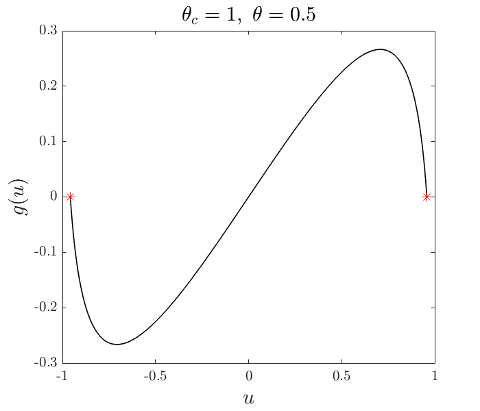
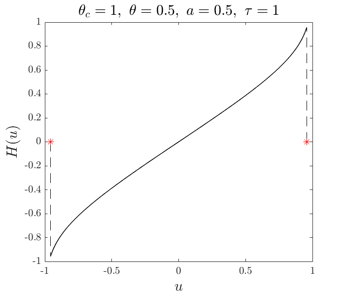
Figure 2. $g(u)$ (left) and $H(u)$ (right) w.r.t. $u\in[-u_{*},u_{*}]$, where $\theta_{c}=1$, $\theta=\frac{1}{2}$, and $a=\frac{1}{2}$. The red star markers denote the nonzero roots of $g$, i.e., $-u_{*}$ and $u_{*}$.

3.1. PR-RK method for approximating $\mathcal{S}_{\mathcal{N}}^{(\mathrm{LOG})}(\tau)$

Diagonally Implicit Runge-Kutta (DIRK) formulae have been widely used for the numerical solution of stiff initial value problems. The simplest method from this class is the second order implicit midpoint method. To approximate $\mathcal{S}_{\mathcal{N}}^{(\mathrm{LOG})}(\tau)v$ for a given function $v$, we shall use the Pareschi and Russo’s two-stage diagonally implicit Runge Kutta (PR-RK) method [13] (see Table 1) . One should note that under the assumption of uniform Sobolev bounds on the numerical iterates, the truncation error involved is guaranteed to be within $\mathcal{O}(\tau^{3})$.

$a$	$a$	$0$
$1-a$	$1-2a$	$a$
	$\frac{1}{2}$	$\frac{1}{2}$

Table 1. Butcher tableau of Pareschi and Russo’s Runge-Kutta method with constant $a$.

More precisely, for given $v$ we approximate $\mathcal{S}_{\mathcal{N}}^{(\mathrm{LOG})}(\tau)v$ via two internal stages (below $a$ is a constant parameter):

$$u_{1}=v+a\tau g(u_{1}),$$ (3.9)

$$u_{2}=v+(1-2a)\tau g(u_{1})+a\tau g(u_{2}),$$

$$\mathcal{S}_{\mathcal{N}}^{(\mathrm{LOG})}(\tau)v\approx\widetilde{\mathcal{S}}_{\mathcal{N}}(\tau)v:=v+\frac{1}{2}\tau g(u_{1})+\frac{1}{2}\tau g(u_{2}).$$

Since the PR-RK method is a second order method, it is not difficult to check that if

$$\max\{\|v\|_{\infty},\,\|u_{1}\|_{\infty},\,\|u_{2}\|_{\infty},\|\widetilde{\mathcal{S}}_{\mathcal{N}}(\tau)v\|_{\infty}\}\leq u_{*}<1,$$ (3.10)

and $v$ has uniform Sobolev bounds, then

$$\mathcal{S}_{\mathcal{N}}^{(\mathrm{LOG})}(\tau)v=\widetilde{\mathcal{S}}_{\mathcal{N}}(\tau)v+\mathcal{O}(\tau^{3}).$$ (3.11)

We shall verify (3.10) later under certain parametric conditions on ($a$, $\theta$, $\theta_{c}$, $\tau$).

Concluding from the above discussion, we are led to the following RK based Strang-type splitting algorithm for (3.1):

$$\boxed{\begin{aligned} &\qquad u^{n+1}=\mathcal{S}_{\mathcal{L}}(\tau/2)\widetilde{\mathcal{S}}_{\mathcal{N}}(\tau)\mathcal{S}_{\mathcal{L}}(\tau/2)u^{n};\\ &\text{In terms of $\tilde{u}^{n}=\mathcal{S}_{\mathcal{L}}(\tau/2)u^{n}$, we have equivalently:}\\ &\qquad\tilde{u}^{n+1}=\mathcal{S}_{\mathcal{L}}(\tau)\widetilde{\mathcal{S}}_{\mathcal{N}}(\tau)\tilde{u}^{n},\end{aligned}}$$ (3.12)

where $\widetilde{\mathcal{S}}_{\mathcal{N}}(\tau)$ is defined via (3.9). We tacitly assume that $\widetilde{\mathcal{S}}_{\mathcal{N}}(\tau)$ is the exact solver of (3.9) and do not consider other intermediate numerical errors due to the implicit nature of the scheme. The validity of this assumption will be examined in the next subsection.

3.2. Solvability of (3.9)

Although the first two equations of (3.9) are implicit, they can be tackled by the Newton method efficiently with quadratic convergence. In practice only a few iterations are needed to achieve machine precision. The first two equations in (3.9) can be rewritten as

$$H(u_{1})-v=0;$$ (3.13)

$$H(u_{2})-v-(1-2a)\tau g(u_{1})=0,$$ (3.14)

where

$$H(u)\coloneqq u-a\tau g(u)=\left(1-a\tau\theta_{c}\right)u+a\tau\theta\operatorname{artanh}(u).$$ (3.15)

See the right plot of Figure 2 for a graphical illustration of $H(u)$.

To solve (3.13), we implement the Newton iteration

$$\begin{cases}u_{1}^{(k+1)}=u_{1}^{(k)}-\frac{H(u_{1}^{(k)})-v}{H^{\prime}(u_{1}^{(k)})},\quad k\geq 0;\\ u_{1}^{(0)}=\mathrm{sign}(v)u_{*}.\end{cases}$$ (3.16)

Similarly, we use the following Newton iteration to solve (3.14)

$$\begin{cases}u_{2}^{(k+1)}=u_{2}^{(k)}-\frac{H(u_{2}^{(k)})-v-(1-2a)\tau g(u_{1})}{H^{\prime}(u_{2}^{(k)})},\quad k\geq 0;\\ u_{2}^{(0)}=\mathrm{sign}(v)u_{*}.\end{cases}$$ (3.17)

Lemma 3.1 (Unique solvability & convergence of Newton iterations).

Assume that $|v|\leq u_{*}$. If $0<\tau\leq\frac{1}{(3a-1)(\theta_{c}-\theta)}$ with $a\geq\frac{1}{2}$, then (3.13) and (3.14) are uniquely solvable, and the Newton iterations (3.16) and (3.17) converge.

Proof.

Without loss of generality, we consider the case when $0<v<u_{*}$. Direct computation gives

$$H^{\prime}(u)=1-a\tau\theta_{c}+\frac{a\tau\theta}{1-u^{2}},\quad H^{\prime\prime}(u)=\frac{2a\tau\theta u}{(1-u^{2})^{2}}.$$ (3.18)

From the condition $0<\tau\leq\frac{1}{(3a-1)(\theta_{c}-\theta)}$ with $a\geq\frac{1}{2}$, we have $0<\tau\leq\frac{1}{a(\theta_{c}-\theta)}$. Thus

$$H^{\prime}(u)>1-a\tau\theta_{c}+a\tau\theta\geq 0,\quad\forall\,0<u\leq u_{*}.\quad\Rightarrow\quad H^{\prime}(u)>0,\qquad\forall\,0<u\leq u_{*}.$$ (3.19)

It is also clear that $H^{\prime\prime}(u)>0$ for any $0<u\leq u_{*}$.

For (3.13), using the fact that $f(u_{*})=0$ we have

$$H(u_{*})-v=u_{*}-v>0,$$ (3.20)

$$H(v)-v=-a\tau g(v)<0.$$

Therefore, (3.13) is uniquely solvable. Given $u_{1}^{(0)}=u_{*}$, it follows that the Newton iteration (3.16) converges to the unique root $u_{1}$ satisfying $v<u_{1}<u_{*}$.

We turn now to (3.14). By using the fact that $g^{\prime}(u)\leq\theta_{c}-\theta$ for $0\leq u<1$, we have $g(u)\leq(\theta_{c}-\theta)u$ for any $0<u<u_{*}$. By using

$$\tau{(3a-1)(\theta_{c}-\theta)}\leq 1,$$ (3.21)

$$g(u)\leq(\theta_{c}-\theta)u,\quad\forall\,0<u<u_{*},$$

we have

$$H(0)-v-(1-2a)\tau g(u_{1})=-u_{1}+(3a-1)\tau g(u_{1})\leq 0,$$ (3.22)

$$H(u_{*})-v-(1-2a)\tau g(u_{1})=u_{*}-v+(2a-1)\tau g(u_{1})>0.$$

Therefore, (3.14) is uniquely solvable. Given $u_{2}^{(0)}=u_{*}$, it follows that the Newton iteration (3.16) converges to some root $0<u_{2}<u_{*}.$ ∎

3.3. The maximum principle

In this subsection, we show that the RK-based Strang-splitting method (3.12) preserves the maximum principle.

Theorem 3.1 (Maximum principle).

Denote by $u_{*}$ the unique root of $g(u)=0$ in $(0,1)$. If $a\geq 1+\frac{\sqrt{2}}{2}$, $0<\tau\leq\frac{1}{(3a-1)(\theta_{c}-\theta)}$, and $\|\tilde{u}^{n}\|_{\infty}\leq u_{*}$, then

$$\|\widetilde{\mathcal{S}}_{\mathcal{N}}(\tau)\tilde{u}^{n}\|_{\infty}\leq u_{*},$$ (3.23)

where $\widetilde{\mathcal{S}}_{\mathcal{N}}(\tau)$ was defined in (3.9). It follows that

$$\|\tilde{u}^{n+1}\|_{\infty}=\|\mathcal{S}_{\mathcal{L}}(\tau)\widetilde{\mathcal{S}}_{\mathcal{N}}(\tau)\tilde{u}^{n}\|_{\infty}\leq u_{*};$$ (3.24)

$$\|u^{n+1}\|_{\infty}=\|\mathcal{S}_{\mathcal{L}}(\tau/2)\widetilde{\mathcal{S}}_{\mathcal{N}}(\tau)\tilde{u}^{n}\|_{\infty}\leq u_{*}.$$ (3.25)

Proof.

It suffices for us to treat $\tilde{u}^{n}$ as a real number. With no loss we consider the case when $0<\tilde{u}^{n}<u_{*}$. As $a\geq 1+\frac{\sqrt{2}}{2}$, we have shown in the proofs of Lemma 3.1 that

$$\tilde{u}^{n}<u_{1}<u_{*}\quad\mbox{and}\quad 0<u_{2}<u_{*}.$$ (3.26)

By (3.9), we have

$$\tau g(u_{1}) =\frac{1}{a}(u_{1}-\tilde{u}^{n});$$ (3.27)

$$\tau g(u_{2}) =\frac{1}{a}(u_{2}-\tilde{u}^{n})-\frac{1}{a}(1-2a)\tau g(u_{1})=\frac{1}{a}(u_{2}-\tilde{u}^{n})-\frac{1}{a^{2}}(1-2a)(u_{1}-\tilde{u}^{n})$$

$$=(\frac{1}{a^{2}}-\frac{3}{a})\tilde{u}^{n}+\frac{1}{a}u_{2}+\frac{2a-1}{a^{2}}u_{1}.$$ (3.28)

Since $a\geq 1+\frac{\sqrt{2}}{2}$, it is not difficult to check that the following inequality holds

$$\frac{3}{2a}-\frac{1}{2a^{2}}\geq 0\quad\mbox{and}\quad 1-\frac{2}{a}+\frac{1}{2a^{2}}\geq 0.$$ (3.29)

Consequently we have

$$\widetilde{\mathcal{S}}_{\mathcal{N}}(\tau)\tilde{u}^{n}=\tilde{u}^{n}+\frac{1}{2}\tau g(u_{1})+\frac{1}{2}\tau g(u_{2})$$ (3.30)

$$\qquad\quad=\frac{1}{2a}u_{2}+\left(\frac{3}{2a}-\frac{1}{2a^{2}}\right)u_{1}+\left(1-\frac{2}{a}+\frac{1}{2a^{2}}\right)\tilde{u}^{n}<u_{*},$$

$$\widetilde{\mathcal{S}}_{\mathcal{N}}(\tau)\tilde{u}^{n}=\tilde{u}^{n}+\frac{1}{2}\tau g(u_{1})+\frac{1}{2}\tau g(u_{2})>\tilde{u}^{n}.$$

It follows that $\|\widetilde{\mathcal{S}}_{\mathcal{N}}(\tau)\tilde{u}^{n}\|_{\infty}<u_{*}.$ More generally, if $\|\tilde{u}^{n}\|_{\infty}\leq u_{*}$, then

$$\|\widetilde{\mathcal{S}}_{\mathcal{N}}(\tau)\tilde{u}^{n}\|_{\infty}\leq u_{*}.$$ (3.31)

Thus

$$\|\tilde{u}^{n+1}\|_{\infty}=\|\mathcal{S}_{\mathcal{L}}(\tau)\widetilde{\mathcal{S}}_{\mathcal{N}}(\tau)\tilde{u}^{n}\|_{\infty}\leq\|\widetilde{\mathcal{S}}_{\mathcal{N}}(\tau)\tilde{u}^{n}\|_{\infty}\leq u_{*}.$$ (3.32)

The bound for $u^{n+1}$ follows similarly. ∎

3.4. Modified energy dissipation

By (3.12), we have

$$e^{-\varepsilon^{2}\tau\Delta}\tilde{u}^{n+1}=\widetilde{\mathcal{S}}_{\mathcal{N}}(\tau)\tilde{u}^{n}.$$ (3.33)

Clearly

$$\frac{1}{\tau}\left(e^{-\varepsilon^{2}\tau\Delta}-1\right)\tilde{u}^{n+1}+\frac{1}{\tau}(\tilde{u}^{n+1}-\tilde{u}^{n})=\frac{1}{\tau}\Bigl{(}\widetilde{\mathcal{S}}_{\mathcal{N}}(\tau)\tilde{u}^{n}-\tilde{u}^{n}\Bigr{)}.$$ (3.34)

By (3.9), we have

$$\frac{1}{\tau}\Bigl{(}\widetilde{\mathcal{S}}_{\mathcal{N}}(\tau)\tilde{u}^{n}-\tilde{u}^{n}\Bigr{)}=\frac{1}{2}g(u_{1})+\frac{1}{2}g(u_{2}).$$ (3.35)

The strategy is to rewrite the RHS above as $-\overline{F}^{\prime}(\tilde{u}^{n})$, where $\overline{F}$ is a one-variable function serving as the potential energy function. For this we need to introduce some notation.

Recall that in (3.9), $u_{1}$ and $u_{2}$ are implicitly defined as a function of $u$ for given $u$. For convenience of notation, we regard $u_{1}=u_{1}(u)$, $u_{2}=u_{2}(u)$ as two smooth functions of $u\in[-u_{*},u_{*}]$ solving

$$u_{1}(u)=u+a\tau g(u_{1}(u)),\quad u_{2}(u)=u+(1-2a)\tau g(u_{1}(u))+a\tau g(u_{2}(u)).$$ (3.36)

We define $\overline{F}=\overline{F}(u)$ as the unique smooth function satisfying

$$\overline{F}^{\prime}(u)=\frac{d}{du}\overline{F}(u)=-\frac{1}{2}g(u_{1}(u))-\frac{1}{2}g(u_{2}(u)),\quad\mbox{with }\overline{F}(0)=0.$$ (3.37)

The normalization $\overline{F}(0)=0$ is chosen in analogy with (1.3) since $F_{\mathrm{fh}}(0)=0$. With the help of $\overline{F}$, we rewrite (3.34) as

$$\frac{1}{\tau}\left(e^{-\varepsilon^{2}\tau\Delta}-1\right)\tilde{u}^{n+1}+\frac{1}{\tau}(\tilde{u}^{n+1}-\tilde{u}^{n})=-\overline{F}^{\prime}(\tilde{u}^{n}).$$ (3.38)

Theorem 3.2 (Modified energy dissipation).

Assume $u^{0}\in H^{1}(\mathbb{T}^{d})$ and $\|u^{0}\|_{\infty}\leq u_{*}$ where $u_{*}$ is the unique root of $g(u)=0$ in $(0,1)$. When $a\geq 1+\frac{\sqrt{2}}{2}$ and $0<\tau\leq\frac{1}{3a(\theta_{c}-\theta)}$, the RK-based Strang splitting method (3.12) preserves the maximum principle and the modified energy dissipation property, namely

$$\sup_{n\geq 1}\max\{\|u^{n}\|_{\infty},\;\|\tilde{u}^{n}\|_{\infty}\}\leq u_{*};$$ (3.39)

$$\overline{E}^{n+1}\leq\overline{E}^{n},\quad\forall\;n\geq 1;$$ (3.40)

$$\overline{E}^{n}\coloneqq\frac{1}{2}\left\langle\frac{1}{\tau}(e^{-\varepsilon^{2}\tau\Delta}-1)\tilde{u}^{n},\tilde{u}^{n}\right\rangle+\left\langle\overline{F}(\tilde{u}^{n}),1\right\rangle,$$ (3.41)

where $\tilde{u}^{n}=\mathcal{S}_{\mathcal{L}}(\tau/2)u^{n}$ and $\overline{F}$ is defined by (3.37).

Remark 3.1.

For the energy dissipation to hold, formally speaking the argument only requires the weaker condition $a\geq\frac{1}{2}$ and $0<\tau\leq\frac{1}{3a(\theta_{c}-\theta)}$. However in order to have solvability of our RK-based scheme for all $n\geq 1$, we need to impose the stronger condition on the parameter $a$ in order to preserve the maximum principle.

Proof.

We only need to show (3.40). Direct computation gives

$$g^{\prime}(u)=\theta_{c}-\frac{\theta}{1-u^{2}}\leq\theta_{c}-\theta,\quad\forall u\in[-u_{*},u_{*}].$$ (3.42)

By (3.37), we have

$$\overline{F}^{\prime\prime}(u)=-\frac{1}{2}g^{\prime}(u_{1})u_{1}^{\prime}(u)-\frac{1}{2}g^{\prime}(u_{2})u_{2}^{\prime}(u),\quad\forall u\in[-u_{*},u_{*}].$$ (3.43)

Taking the derivative of two equations in (3.36) w.r.t. $u$, we have

$$u_{1}^{\prime}(u)=\frac{1}{1-a\tau g^{\prime}(u_{1})},$$ (3.44)

$$u_{2}^{\prime}(u)=\frac{(3-\frac{1}{a})-(2-\frac{1}{a})u_{1}^{\prime}(u)}{1-a\tau g^{\prime}(u_{2})}.$$

By (3.42) and the assumption $0<\tau\leq\frac{1}{3a(\theta_{c}-\theta)}$, we have

$$g^{\prime}(u)\leq\theta_{c}-\theta\leq\frac{1}{3a\tau},\quad\forall\,u\in[-u_{*},u_{*}].$$ (3.45)

This yields

$$0<u_{1}^{\prime}(u)\leq\frac{3}{2}\quad\mbox{and}\quad\left(3-\frac{1}{a}\right)-\left(2-\frac{1}{a}\right)u_{1}^{\prime}(u)>0.$$ (3.46)

Substituting (3.44) into (3.43), we then have

$$\overline{F}^{\prime\prime}(u) =-\frac{1}{\frac{2}{g^{\prime}(u_{1})}-2a\tau}-\frac{(3-\frac{1}{a})-(2-\frac{1}{a})u_{1}^{\prime}(u)}{\frac{2}{g^{\prime}(u_{2})}-2a\tau}$$ (3.47)

$$\leq\frac{1}{2a\tau}+\frac{3-\frac{1}{a}}{2a\tau}=\frac{4-\frac{1}{a}}{2a\tau}\leq\frac{2}{\tau},\qquad\forall u\in[-u_{*},u_{*}].$$

Multiplying (3.38) with $(\tilde{u}^{n+1}-\tilde{u}^{n})$ and integrating over $\mathbb{T}^{d}$, we obtain

$$\overline{E}^{n+1}-\overline{E}^{n}\leq-\left\langle\left(\frac{1}{\tau}-\frac{1}{2}\overline{F}^{\prime\prime}(\xi^{n})\right)(\tilde{u}^{n+1}-\tilde{u}^{n})^{2},1\right\rangle\leq 0,$$ (3.48)

where $-u_{*}\leq\xi^{n}\leq u_{*}$ is some function between $\tilde{u}^{n}$ and $\tilde{u}^{n+1}$. ∎

Remark 3.2.

The restrictions on ($a$, $\tau$) in Theorem 3.1 and 3.2 do not depend on $\sup_{|u|\leq u_{*}}|g^{\prime}(u)|$ which could be very large.

We now complete the proof of Theorem 1.2.

Proof of Theorem 1.2.

The first two statements follow from Theorem 3.2. The rest of the statements can be proved along similar lines as in Theorem 1.1. We omit the details. ∎

4. Numerical results

In this section, we implement the Strang splitting methods on the AC equation (2.34) and (3.1) with periodic boundary conditions.

Space discretization. We use the spectral method to compute the linear solution operator $\mathcal{S}_{\mathcal{L}}(\tau)$ in the Strang splitting method. Suppose that $\Omega=[0,L]^{2}$ with $L>0$ is a periodic torus. We can compute $e^{t\Delta_{h}}u$ via fast Fourier transform (FFT) as follows. Denote by $\Delta_{h}$ the discrete Laplacian operator with $h=\frac{L}{N}$ and $N\geq 1$ being an integer. We use the following convention for FFT:

$$u_{\mathbf{j}}=\sum_{-\frac{N}{2}<k_{x},k_{y}\leq\frac{N}{2}}\hat{u}_{\mathbf{k}}\,e^{\frac{2\pi i}{N}\mathbf{j}\cdot\mathbf{k}},$$ (4.1)

$$\hat{u}_{\mathbf{k}}=\frac{1}{N^{2}}\sum_{j_{x},j_{y}=0}^{N-1}u_{\mathbf{j}}\,e^{-\frac{2\pi i}{N}\mathbf{j}\cdot\mathbf{k}},$$ (4.2)

where $\mathbf{j}=(j_{x},j_{y})$ and $\mathbf{k}=(k_{x},k_{y})$. We have

$$(\Delta_{h}u)_{\mathbf{j}}=\frac{u_{j_{x},j_{y}+1}+u_{j_{x},j_{y}-1}+u_{j_{x}+1,j_{y}}+u_{j_{x}-1,j_{y}}-4u_{j_{x},j_{y}}}{h^{2}}.$$ (4.3)

Clearly

$$(\widehat{\Delta_{h}u})_{\mathbf{k}}=w_{\mathbf{k}}\hat{u}_{\mathbf{k}},\quad-\frac{N}{2}<k_{x},k_{y}\leq\frac{N}{2},$$ (4.4)

where

$$w_{\mathbf{k}}=h^{-2}\left(2\cos\left(2\pi\frac{k_{x}}{N}\right)+2\cos\left(2\pi\frac{k_{y}}{N}\right)-4\right).$$ (4.5)

It follows that

$$\widehat{(\mathcal{S}_{\mathcal{L}}(\tau)u)}_{\mathbf{k}}=\widehat{(e^{\varepsilon^{2}\tau\Delta_{h}}u)}_{\mathbf{k}}=e^{\varepsilon^{2}\tau w_{\mathbf{k}}}\hat{u}_{\mathbf{k}},\quad-\frac{N}{2}<k_{x},k_{y}\leq\frac{N}{2}.$$ (4.6)

Taking the inverse fast Fourier transform (IFFT) then produces the numerical values of $\mathcal{S}_{\mathcal{L}}(\tau)u$ on the real side.

Similarly we compute $e^{-\varepsilon^{2}\tau\Delta}u$ in the definition of modified energy by taking the IFFT of the following equation

$$\widehat{(e^{-\varepsilon^{2}\tau\Delta_{h}}u)}_{\mathbf{k}}=e^{-\varepsilon^{2}\tau w_{\mathbf{k}}}\hat{u}_{\mathbf{k}},\quad-\frac{N}{2}<k_{x},k_{y}\leq\frac{N}{2}.$$ (4.7)

In the following numerical tests, we use the above spectral method for space discretization.

4.1. 2D Allen–Cahn with polynomial potential

Consider the AC equation (2.34) with polynomial potential, where $\varepsilon=0.1$ and the $2\pi$-periodic domain $\Omega=[0,2\pi]^{2}$. We take the initial data $u_{0}$ as

$$u_{0}(x,y)=0.05\sin(x)\sin(y).$$ (4.8)

We use $N\times N=512\times 512$ Fourier modes for the space discretization.

Since the exact PDE solution is not available, we take a small splitting step $\tau=10^{-4}$, to obtain an “almost exact” solution $u_{\mathrm{ex}}$ at time $T=20$. Then, we take several different splitting steps $\tau=\frac{1}{10}\times 2^{-k}$ with $k=0,1,\ldots,4$ and obtain corresponding numerical solutions at $T=20$. The $\ell_{2}$-errors between these solutions and the “almost exact” solution are summarized in Table 2. Reassuringly, it is observed that the convergence rate is about $2$, i.e. the scheme has second order in-time accuracy.

Table 2. $\ell_{2}$-errors of numerical solutions to the AC equation (2.34) with polynomial potential at time $T=20$ for different splitting steps.

  $\tau$ $\frac{1}{10}$ $\frac{1}{20}$ $\frac{1}{40}$ $\frac{1}{80}$ $\frac{1}{160}$ $\ell_{2}$-error $9.367\times 10^{-4}$ $2.345\times 10^{-4}$ $5.865\times 10^{-5}$ $1.466\times 10^{-5}$ $3.665\times 10^{-6}$ rate – $1.998$ $1.999$ $2.000$ $2.000$  

In Figure 3 we plot the standard energy versus the modified energy as a function of time. The time step is $\tau=0.01$. It is observed that the standard energy and the modified energy coincide approximately, and they both decay monotonically in time.

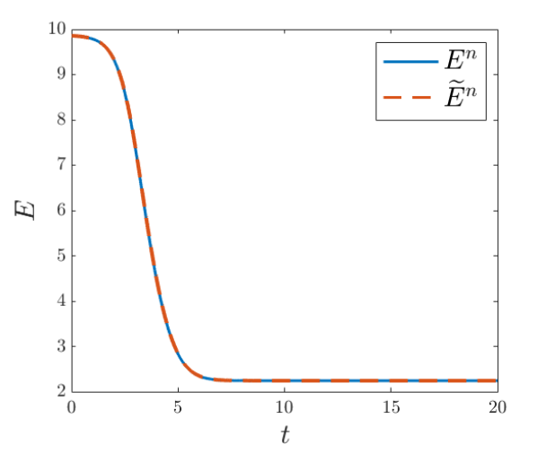
Figure 3. Standard energy $E^{n}$ and modified energy $\widetilde{E}^{n}$ w.r.t. time for the Strang splitting method, with splitting step $\tau=0.01$ and number of Fourier modes $512\times 512$.

4.2. 2D AC with the logarithmic potential

Consider the AC equation (3.1) with logarithmic potential, where $\varepsilon=0.01$, $\theta_{c}=1$ and $\theta=\frac{1}{4}$. The spatial domain is the two-dimensional $2\pi$-periodic torus $\Omega=[0,2\pi]^{2}$. We take the initial condition $u_{0}$ as

$$u_{0}(x,y)=0.5\left[\chi\left((x-\pi)^{2}+(y-\pi)^{2}\leq 1.2\right)-0.5\right],$$ (4.9)

where $\chi$ is the characteristic function. We employ the RK-based Strang splitting method (3.12) to solve this equation. The tolerance threshold of the Newton iterative solver is set to be $10^{-12}$. We use the standard Fourier spectral method with $512\times 512$ Fourier modes for the space discretization.

As a first step, we test the convergence rate of the RK-based Strang splitting method. In Table 2, we show the $\ell_{2}$-errors of the numerical solution at $T=1$, where the parameter $a$ in the PR-RK method is set to $a=1+\frac{\sqrt{2}}{2}$. As before, the “exact” solution is taken as the numerical solution when $\tau=10^{-4}$. It can be observed that the convergence order is about $2$.

Table 3. $\ell_{2}$-errors of numerical solutions at time $T=1$ to the AC equation with logarithmic potential (3.1) for different splitting steps, computed by the RK-based Strang splitting method with $a=1+\frac{\sqrt{2}}{2}$.

  $\tau$ $\frac{1}{10}$ $\frac{1}{20}$ $\frac{1}{40}$ $\frac{1}{80}$ $\frac{1}{160}$ $\ell_{2}$-error $2.245\times 10^{-2}$ $4.935\times 10^{-3}$ $1.160\times 10^{-3}$ $2.815\times 10^{-4}$ $6.933\times 10^{-5}$ rate – $2.186$ $2.088$ $2.043$ $2.022$  

Secondly, we test the convergence rate for an interesting case of $a=\frac{1}{2}+\frac{\sqrt{3}}{6}$, where the PR-RK method in Table 1 becomes the Crouzeix’s third order RK method. In this case the approximation error of nonlinear solution operator becomes $\mathcal{O}(\tau^{4})$, i.e.,

$$\mathcal{S}_{\mathcal{N}}(\tau)\tilde{u}^{n}=\widetilde{\mathcal{S}}_{\mathcal{N}}(\tau)\tilde{u}^{n}+\mathcal{O}(\tau^{4}).$$ (4.10)

On the other hand, the overall error of the method (3.9) is still second order in time. Interestingly, the numerical results in Table 4 show that the convergence rate for $a=\frac{1}{2}+\frac{\sqrt{3}}{6}$ appears to be higher than the corresponding case of $a=1+\frac{\sqrt{2}}{2}$ in Table 3. This is probably due to the inaccuracy of the reference solution which was taken as the $\tau=10^{-4}$-almost exact-solution.

Table 4. $\ell_{2}$-errors of numerical solutions at time $T=1$ to the AC equation with logarithmic potential (3.1) for different splitting steps, computed by the RK-based Strang splitting method with $a=\frac{1}{2}+\frac{\sqrt{3}}{6}$.

  $\tau$ $\frac{1}{10}$ $\frac{1}{20}$ $\frac{1}{40}$ $\frac{1}{80}$ $\frac{1}{160}$ $\frac{1}{320}$ $\ell_{2}$-error $9.440\times 10^{-5}$ $1.132\times 10^{-5}$ $1.392\times 10^{-6}$ $1.750\times 10^{-7}$ $2.286\times 10^{-8}$ $3.302\times 10^{-9}$ rate – $3.060$ $3.023$ $2.992$ $2.936$ $2.792$  

Finally, we test the maximum principle and the energy dissipation of the RK-based Strang splitting method. We set $a=1+\frac{\sqrt{2}}{2}$ and $\tau=0.01$, so that the restrictions in Theorem 3.1 and 3.2 are satisfied. Numerical solutions up to $t=10$ are illustrated in Figure 5. It can be observed that $\|u\|_{\infty}$ is always less than $u_{*}\approx 0.99933$, i.e., the maximum principle holds. In Figure 5, we plot the standard energy $E^{n}$ w.r.t. time which clearly decays in time. Note that the modified energy $\overline{E}^{n}$ is implicit in this case and is not plotted here.

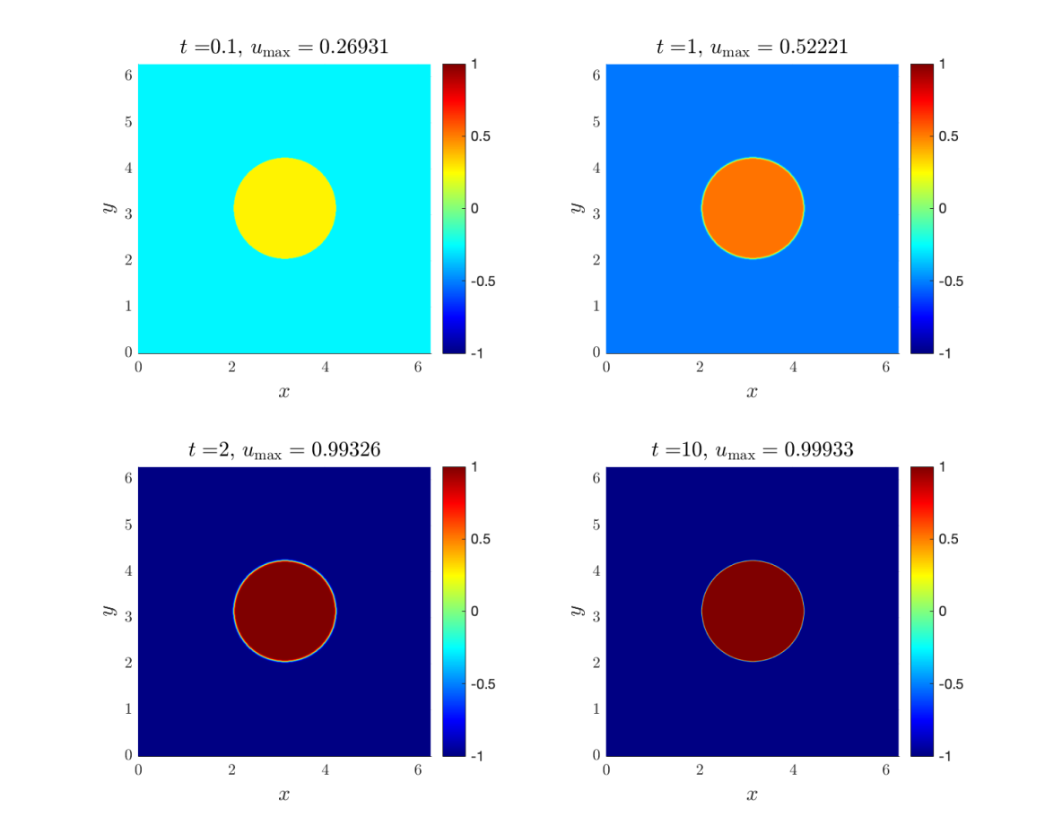
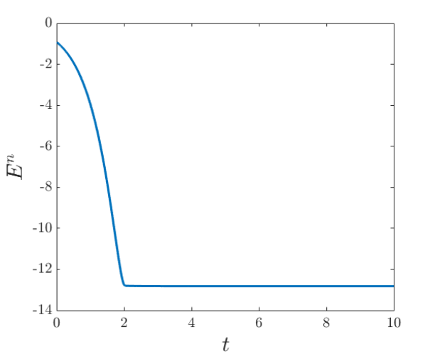
Figure 4. Numerical solution to the AC equation with logarithmic potential computed by the RK-based Strang splitting method with splitting step $\tau=0.01$ and number of Fourier modes $512\times 512$. $u_{\mathrm{max}}$ denotes the maximal absolute value of $u$.

Figure 5. Standard energy w.r.t. time for the RK-based Strang splitting method (3.12) with splitting step $\tau=0.01$ and number of Fourier modes $512\times 512$.

4.3. Seven circles

Consider the AC equation (3.1) with $\varepsilon=0.1$, $\theta_{c}=1$ and $\theta=\frac{1}{4}$. The domain is the two-dimensional $2\pi$-periodic torus $\Omega=[0,2\pi]^{2}$. The initial condition consists of seven circles with centers and radii given in Table 5:

$$u_{0}(x,y)=-1+\sum_{i=1}^{7}f_{0}\left(\sqrt{(x-x_{i})^{2}+(y-y_{i})^{2}}-r_{i}\right),$$ (4.11)

where

$$f_{0}(s)=\left\{\begin{aligned} &2e^{-\varepsilon^{2}/s^{2}}&&\mbox{if }s<0,\\ &0&&\mbox{otherwise.}\end{aligned}\right.$$ (4.12)

Table 5. Centers $(x_{i},y_{i})$ and radii $r_{i}$ in the initial condition (4.11).

  $i$ 1 2 3 4 5 6 7 $x_{i}$ $\pi/2$ $\pi/4$ $\pi/2$ $\pi$ $3\pi/2$ $\pi$ $3\pi/2$ $y_{i}$ $\pi/2$ $3\pi/4$ $5\pi/4$ $\pi/4$ $\pi/4$ $\pi$ $3\pi/2$ $r_{i}$ $\pi/5$ $2\pi/15$ $2\pi/15$ $\pi/10$ $\pi/10$ $\pi/4$ $\pi/4$  

We use the RK-based Strang splitting method with $a=1+\frac{\sqrt{2}}{2}$ and $\tau=0.01$ to solve this equation with the Newton iterative solver. To achieve mediocre accuracy the tolerance threshold for the Newton iteration is set as $10^{-12}$ which is close to the machine precision. We employ the spectral method with $512\times 512$ Fourier modes for the space discretization. The evolution of phase field is illustrated in Figure 7, where the annihilation of the circles take place gradually in time. The corresponding energy evolution is recorded in Figure 7.

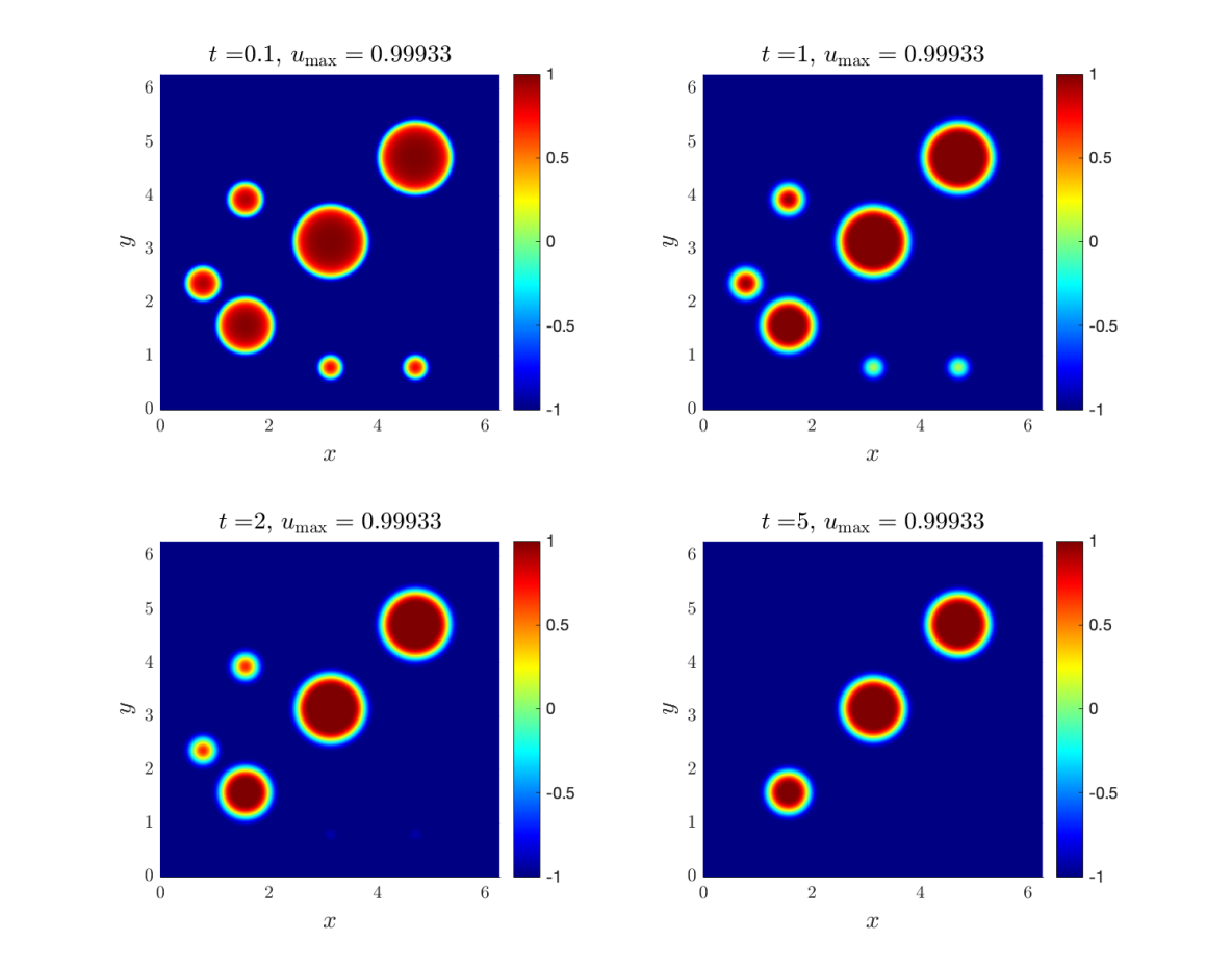
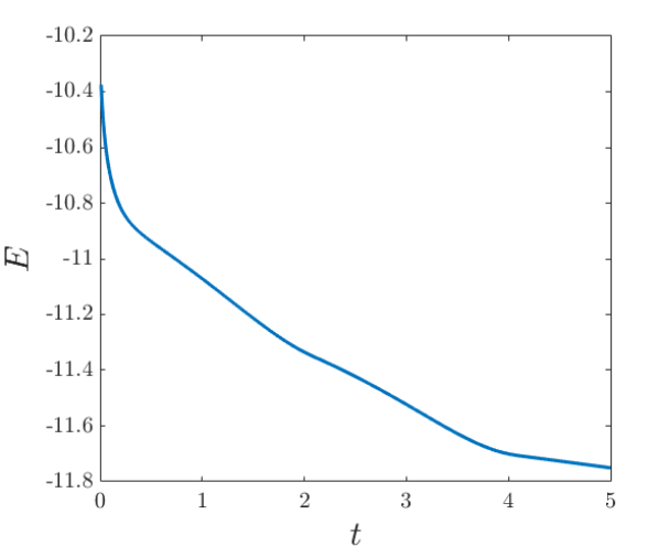
Figure 6. Numerical solution of the seven circles example computed by the RK-based Strang splitting method with splitting step $\tau=0.01$ and number of Fourier modes $512\times 512$. $u_{\mathrm{max}}$ denotes the maximal absolute value of $u$.

Figure 7. Standard energy w.r.t. time for the RK-based Strang splitting method (3.12) in the seven circles example with splitting step $\tau=0.01$ and number of Fourier modes $512\times 512$.

5. Conclusion

In this work we investigated a class of second-order Strang splitting methods for Allen-Cahn equations with polynomial and logarithmic nonlinearities. For the polynomial case we compute both the linear and the nonlinear propagators explicitly. Unconditional stability is established for any time step $\tau>0$. For a judiciously modified energy which coincides with the classical energy up to $O(\tau)$, we show strict energy dissipation and obtain uniform control of higher Sobolev norms. For the logarithmic potential case, since the continuous-time nonlinear propagator no longer enjoys explicit analytic treatments, we adopted a second order in time two-stage implicit Runge–Kutta (RK) nonlinear propagator together with an efficient Newton iterative solver. We establish a sharp maximum principle which ensures phase separation. We prove a new modified energy dissipation law under very mild restrictions on the time step. The methods introduced in this work can be generalized to many other models including nonlocal Allen-Cahn models, Cahn–Hilliard equations, general drift-diffusion systems and nonlinear parabolic systems.

References

[1]
Samuel M Allen and John W Cahn.
A microscopic theory for antiphase boundary motion and its
application to antiphase domain coarsening.
Acta Metallurgica, 27(6):1085–1095, 1979.
[2]
Paul J Flory.
Thermodynamics of high polymer solutions.
The Journal of Chemical Physics, 10(1):51–61, 1942.
[3]
Maurice L Huggins.
Solutions of long chain compounds.
The Journal of Chemical Physics, 9(5):440–440, 1941.
[4]
Yuanzhen Cheng, Alexander Kurganov, Zhuolin Qu, and Tao Tang.
Fast and stable explicit operator splitting methods for phase-field
models.
Journal of Computational Physics, 303:45–65, 2015.
[5]
Zhifeng Weng and Longkun Tang.
Analysis of the operator splitting scheme for the allen–cahn
equation.
Numerical Heat Transfer, Part B: Fundamentals, 70(5):472–483,
2016.
[6]
Weizhu Bao, Shi Jin, and Peter A Markowich.
On time-splitting spectral approximations for the Schrödinger
equation in the semiclassical regime.
Journal of Computational Physics, 175(2):487–524, 2002.
[7]
Mechthild Thalhammer.
Convergence analysis of high-order time-splitting pseudospectral
methods for nonlinear Schrödinger equations.
SIAM Journal on Numerical Analysis, 50(6):3231–3258, 2012.
[8]
Stéphane Descombes.
Convergence of a splitting method of high order for
reaction-diffusion systems.
Mathematics of Computation, 70(236):1481–1501, 2001.
[9]
Su Zhao, Jeremy Ovadia, Xinfeng Liu, Yong-Tao Zhang, and Qing Nie.
Operator splitting implicit integration factor methods for stiff
reaction–diffusion–advection systems.
Journal of Computational Physics, 230(15):5996–6009, 2011.
[10]
Gilbert Strang.
On the construction and comparison of difference schemes.
SIAM Journal on Numerical Analysis, 5(3):506–517, 1968.
[11]
Guri I Marchuk.
Splitting and alternating direction methods.
Handbook of Numerical Analysis, 1:197–462, 1990.
[12]
Yibao Li, Hyun Geun Lee, Darae Jeong, and Junseok Kim.
An unconditionally stable hybrid numerical method for solving the
Allen–Cahn equation.
Computers & Mathematics with Applications, 60(6):1591–1606,
2010.
[13]
Lorenzo Pareschi and Giovanni Russo.
Implicit–explicit Runge–Kutta schemes and applications to
hyperbolic systems with relaxation.
Journal of Scientific Computing, 25(1):129–155, 2005.
[14]
B. Li, J. Yang, and Z. Zhou. Arbitrarily high-order exponential cut-off methods for preserving maximum principle of parabolic equations. SIAM Journal on Scientific Computing 42, no. 6 (2020): A3957–A3978.
[15]
D. Li and C. Quan.
The operator-splitting method for Cahn-Hilliard is stable.
arXiv:2107.01418, 2021.
[16]
D. Li and C. Quan.
On the energy stability of Strang-splitting for Cahn-Hilliard.
arXiv:2107.05349, 2021.
[17]
D. Li and C. Quan.
Negative time splitting is stable. arXiv:2107.07332, 2021.
[18]
D. Li.
Effective maximum principles for spectral methods.
Ann. Appl. Math., 37 (2021), pp. 131–290.
[19]
D. Li, T. Tang, Stability of the Semi-Implicit Method for the Cahn-Hilliard Equation with Logarithmic Potentials. Ann. Appl. Math., 37 (2021), p. 31–60.
[20]
B. Li and Y. Wu: A fully discrete low-regularity integrator for the 1D periodic cubic nonlinear
Schrödinger equation.
Numer. Math. (to appear), arXiv:2101.03728