A new experiment for the gravitational waves detection

Abstract

A new experiment for the gravitational waves (GWs) detection is proposed. It is indeed shown that the effect of GWs on sound waves (SWs) in a fluid is that GWs vary the pressure of the fluid by crossing it. This variation can be found by analysing the gauge of the local observer. It is shown that one can, in principle, detect GWs through the proposed new experiment. The variation of the pressure of the fluid, which represents detected signals, are indeed much higher than the correspondent values of GWs amplitudes. The examples of rotating neutron stars (NSs) and relic GWs are discussed. Remarkably, a confrontation of the proposed new method with a previous paper of Singh et al. on a similar approach shows a possible improvement of the sensitivity concerning the potential detection of GWs. It must be emphasized that this proposed procedure may be difficult in practical experiments because of the presence of different types of noise. For this reason, a Section of the paper is dedicated to the discussion of such noises. On the other hand, this paper must be considered as being pioneering in the new proposed approach. Thus, we hope in future, more precise studies of the noise which concerns the proposed new experiment will be done.

I Introduction

Gravitational waves (GWs) emissions were indirectly discovered from the compact binary system PSR1913+16, composed by two neutron stars (NSs) 1 . Such a discovery, which permitted to award the Nobel Prize of Physics in 1993 to Russell Hulse and Joseph Taylor, excited interest in GWs science despite the first efforts at direct GWs detection started before it 2 . Those efforts involved the design, implementation, and advancement of extremely sophisticated GWs detection technology which is requested by researchers working in this field of research 2 . The most important reason for GWs research is, to use GWs as a probe of the systems that produce them. The famous event GW150914, which is the first observation of GWs from a binary black hole (BH) merger 3 occurred in the 100th anniversary of Albert Einstein’s prediction of GWs 4 . That event was a cornerstone for science in general and for gravitational physics in particular. Indeed it gave definitive proof of the existence of GWs, the existence of BHs that having mass greater than 25 solar masses and the existence of binary systems of BHs which merge in a time less than the age of the Universe 3 . Such a direct GWs discovery, represented the starting of the new era of the GWs astronomy and it enabled Rainer Weiss, Barry Barish and Kip Thorne to win the Nobel Prize of Physics in 2017 . After the event GW150914, the LIGO Scientific Collaboration announced other new GWs detections 5 .

There are lot of experiments for the direct GWs detection with different methods. Ground-based laser interferometers like Advanced LIGO 6 , VIRGO 7 , GEO 8 , TAMA9 , DECIGO 10 , AIGO 11 and space-based laser interferometers like LISA 12 , eLISA 13 and Big Bang Observer 14 which are the most famous. This kind of GWs detectors could be, in principle decisive to confirm the physical consistence of the general theory of relativity (GTR) or alternatively to endorse the framework of extended theories of gravity 15 ; 16 . In fact, some differences between the GTR and alternative theories can be pointed out in the linearized theory of gravity through different interferometer response functions 15 ; 16 . A controversial issue on a potential GWs consists in the detection of the B-modes of the polarization of the cosmic microwave background 17 . More precise measures will be needed to confirm such a GWs in the future 18 . Other attempts are based on measurements of polarization of electromagnetic waves 19 ; 20 and on maser beam passing through a strong static magnetic field 21 ; 22 . But based on the weakness of GWs amplitudes, researchers prefer using laser interferometer technology 5 ; 6 . Also there is another method that analysed the sensitivity to continuous-wave strain fields of a kg-scale optomechanical system formed by the acoustic motion of super fluid helium-4 parametrically coupled to a superconducting microwave cavity, see a1 for more details. But again the sensitivity based on this method was low.

Therefore in this paper, we attempt to introduce another experiment for a potential GWs detection. The gravity effect of GWs on longitudinal waves like sound waves (SWs) in a fluid will be considered. GWs perturb the shape of SWs and this perturbation can vary the pressure in the fluid. The effect of this perturbation can be found by solving the geodesic equation. Remarkably, the estimated amounts of the pressure based on this perturbation are much higher than the strain sensitivity of GWs interferometers and another methods. For examples a confrontation of the proposed new method in a1 on a similar approach shows a possible improvement of the sensitivity concerning the potential detection of GWs, The key point is that one can find superposition in the intersection points between the two types of wave. Such a superposition causes a variation in the SWs pressure. Thus GWs can be in principle, detected by measuring this perturbation.

The paper is organized as it follows. In Sec. 2, SWs will be reviewed. In Sec. 3, the set up of GWs detection will be analysed by considering the perturbation on SWs. In Sec. 4, the different sources of noises will be investigated and in Sec. 5 the conclusion remarks will be discussed.

II Sound waves

Plane waves such as SWs are longitudinal waves that require a material medium (a fluid) to exist. We start to review the driving of plane waves in the fluid in brief. Some parameters will be used as it follows:

$x\equiv$coordinate of the particle in its situation of equilibrium;

$w\equiv$variation of the particle with respect to $x$;

$u_{x}\equiv\frac{\partial w}{\partial t}\equiv$instant speed of particle;

$\rho_{0}\equiv$density of fluid in its situation of equilibrium;

$P\equiv$instant pressure of each point of the fluid;

$P_{0}\equiv$pressure of the fluid in it’s situation of equilibrium;

$p\equiv dP=P-P_{0}\equiv$variation of the pressure;

$\gamma\equiv$speed of propagation of the wave.

In this paper, we define “a particle” as being a small volume of the fluid if one can assume that there is no variation for the pressure, density and speed of all molecules of that volume. In addition, we consider the following assumptions for measuring the variation of pressure:

• for the sake of simplicity, the fluid must be homogeneous, isotropic and elastic;

• in order to consider the effect of GWs on SWs, the amplitude of SWs must be small;

• also for same reason, the variation of the density must be small with respect to the its value at the equilibrium, see tables. [1,2] in Sec.(3) for some numerical examples of pressure.

Then, let us consider a layer of the fluid in equilibrium state with a vertical section $S$ between two parallel surfaces with positions $x$ and $x+dx$, see Fig.[1].

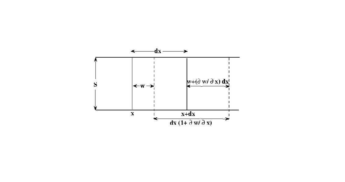
Figure 1: The variation of the longitudinal positions of the plane wave in the fluid.

Therefore, the mass of this layer is $\rho_{0}Sdx$. Now, let us suppose this layer moves to $w,w+\left(\frac{\partial w}{\partial x}\right)dx$ due to right - pass wave. Because the pressures on the both sides of layer are not equal, therefore there exists a force that moves the mass of the layer $\rho_{0}Sdx$ to the right side as it follows:

$$dF_{x}=[p-(p+\frac{\partial p}{\partial x}dx)]S=-\frac{\partial p}{\partial x}dxS.$$ (1)

This force causes an acceleration $\frac{\partial^{2}w}{\partial t^{2}}$. Then from Newtons second law with $m=\rho_{0}dxS$, one gets

$$-\frac{\partial p}{\partial x}=\rho_{0}\frac{\partial^{2}w}{\partial t^{2}}.$$ (2)

There is another relation for the pressure (see Appendix.[A] for more details):

$$p=-\rho_{0}\gamma^{2}\frac{\partial w}{\partial x}.$$ (3)

By combining Eqs. (2) and (3) one gets the plan wave equations:

$$\frac{\partial^{2}w}{\partial t^{2}}=\gamma^{2}\frac{\partial^{2}w}{\partial x^{2}}$$ (4)

$$\frac{\partial^{2}p}{\partial t^{2}}=\gamma^{2}\frac{\partial^{2}p}{\partial x^{2}},$$ (5)

where the speed of propagation of the wave $\gamma$ is given by $\left(\frac{dP}{d\rho}\right)_{0}$ 23 .

III The effect of gravitational waves on sound waves

In order to rigorously derive the effect of GWs on SWs, one needs to perform the fluid dynamics calculation shown in Section 2 in the space-time of the GWs. The calculation shown in Section 2 was indeed performed with the implicit assumption of Minkowskian space-time. In a weak gravitational field (which is the GWs case), the metric is almost Minkowskian 24

$$g_{\mu\nu}=\eta_{\mu\nu}+h_{\mu\nu},$$ (6)

where $\eta_{\mu\nu}$ is the standard metric tensor of the flat Minkowskian space-time (In this space-time, Lorentz transformations can be visualized as ordinary rotations of the four dimensional Euclidean sphere $x^{2}+y^{2}+z^{2}-c^{2}t^{2}=$ constant, where c is the speed of light) and $h_{\mu\nu}\ll 1$ is the weak GWs perturbation 24 . Also the $h_{\mu\nu}$ satisfy the linearized Einstein equation $\square h_{\mu\nu}=0$ 24 . By assuming that GWs travel in the $z-$direction, in the TT-gauge the line element which describes the plane polarized GWs propagating in flat space-time is given by 24

$$h_{\mu\nu}=\left(\begin{array}[]{cccc}0&0&0&0\\ 0&h_{+}&h_{\times}&0\\ 0&h_{\times}&-h_{+}&0\\ 0&0&0&0\end{array}\right)\exp[i(kz-\omega t)],\;\;\;\;\omega=kc,$$ (7)

where $h_{+}$ and $h_{\times}$ are the two standard GWs polarizations. For astrophysical sources it should be $h_{+}\thickapprox h_{\times}\leq 10^{-21}$ 3 , 25 -29 .

On the other hand, as GWs detection is performed in a laboratory environment on Earth, one typically uses the coordinate system in which space-time is locally flat and the distance between any two points is given simply by the difference in their coordinates in the sense of Newtonian physics. This is the so-called gauge of the local observer 15 ; 24 . In such a gauge the GWs manifest themselves by exerting tidal forces on the test masses (here we consider “particles”, i.e. small volumes of the fluid). By putting a particle in the origin of the coordinate system, the components of the separation vector are the coordinates of the second particle. The effect of the GWs is to drive this particle to have oscillations. Equivalently we can say that there is a gravitational potential which generates the tidal forces 24

$$V(\overrightarrow{r},t)=-\frac{1}{4}\ddot{h}_{+}(t)[x^{2}-y^{2}],$$ (8)

and that the motion of the particle is governed by the Newtonian equation

$$\ddot{\overrightarrow{r}}=-\bigtriangledown V.$$ (9)

In geometric terms the connection between Newtonian theory and linearized general relativity are given by the relation between the gravitational potential and the time component of the metric 313

$$g_{00}=-1-\frac{2V}{c^{2}}.$$ (10)

The equations of motion for the particle in the gauge of the local observer are well known 24

$$\ddot{x}=\frac{1}{2}\ddot{h}_{+}x$$ (11)

$$\ddot{y}=-\frac{1}{2}\ddot{h}_{+}y.$$ (12)

Thus, setting

$$-\frac{\partial p_{1}}{\partial x}\equiv\frac{1}{2}\rho_{0}\ddot{h}_{+}x;\qquad\ddot{x}\equiv\frac{\partial^{2}w_{1}}{\partial t^{2}},$$ (13)

one gets the total perturbation (GWs plus SWs) as

$$-\frac{\partial p}{\partial x}-\frac{\partial p_{1}}{\partial x}=\rho_{0}\frac{\partial^{2}w}{\partial t^{2}}+\rho_{0}\frac{\partial^{2}w_{1}}{\partial t^{2}},$$ (14)

where $p_{1}$ and $w_{1}$ are the pressure and the variation of the position of the particle due to the GWs presence respectively. (We note that $\partial x$ should be replaced by $\partial x\sqrt{1+h_{+}}$ in the GWs case. But as it is $h_{+}\ll 1$ , this will not affect our results. Therefore, we can ignore it.) Now, setting

$$p_{h_{+}}\equiv p+p_{1};\qquad w_{h_{+}}\equiv w+w_{1},$$ (15)

Then Eqs. (2), (3), (4), (5), change as

$$-\frac{\partial\left(p_{h_{+}}\right)}{\partial x}=\rho_{0}\frac{\partial^{2}\left(w_{h_{+}}\right)}{\partial t^{2}}$$ (16)

$$p_{h_{+}}=-\rho_{0}\gamma^{2}\frac{\partial\left(w_{h_{+}}\right)}{\partial x}$$ (17)

$$\frac{\partial^{2}\left(w_{h_{+}}\right)}{\partial t^{2}}=\gamma^{2}\frac{\partial^{2}\left(w_{h_{+}}\right)}{\partial x^{2}}$$ (18)

$$\frac{\partial^{2}\left(p_{h_{+}}\right)}{\partial t^{2}}=\gamma^{2}\frac{\partial^{2}\left(p_{h_{+}}\right)}{\partial x^{2}},$$ (19)

Now, combining Eq. (11) with the second definition in Eq. (13), one gets

$$\frac{\partial^{2}w_{1}}{\partial t^{2}}=\frac{1}{2}\ddot{h}_{+}x=\frac{1}{2}\omega^{2}h_{0+}x\cos\left(kz-\omega t\right),$$ (20)

where

$$\begin{array}[]{c}h_{+}\equiv h_{0+}\cos\left(kz-\omega t\right),\\ \\ \end{array}$$

Thus, one gets the solution for $w_{1}$ as

$$w_{1}=\frac{1}{2}xh_{0+}\left[-\cos\left(kz-\omega t\right)+\cos kz+\omega t\sin kz\right].$$ (21)

One gets also

$$\begin{array}[]{c}p_{1}=-\rho_{0}\gamma^{2}\frac{\partial w_{1}}{\partial x}=\\ \\ \frac{1}{2}\rho_{0}\gamma^{2}h_{0+}\left[\cos\left(kz-\omega t\right)-\cos kz-\omega t\sin kz\right].\end{array}$$ (22)

From Eq. (15) one can see that, in the GWs absence, that is $h_{0+}=0$, then $p_{h_{+}}=p$, and $w_{h_{+}}=w.$ Setting $\cos\left(kz-\omega t\right)=1$ for the sake of simplicity, one writes

$$\begin{array}[]{c}\Delta p\equiv p_{h_{+}}-p=\\ \\ \frac{1}{2}\rho_{0}\gamma^{2}h_{0+}\left[1-\left(\cos kz+\omega t\sin kz\right)\right].\end{array}$$ (23)

Now, we will see that from this last relation one can, in principle detect the effect of GWs. But, in practice the presence of different types of noise may cause some problems for realizing this kind of GWs detection. This issue will be discussed in next Section. On the other hand, we stress that this paper must be considered as being pioneering in the new proposed approach. Thus, we hope in future, more precise studies of the noise which concerns the proposed new experiment.

One also notes that GWs and SWs are two different waves with transversal and longitudinal properties respectively. Thus, one cannot merely realize a superposition between the two different types of waves. Hence, starting from Eq. (14), all the equations involving the total perturbation (GWs plus SWs) are satisfied only for the intersection points between GWs and SWs, see Fig.[2]. In other words, GWs cause perturbation in the SWs shape. The perturbation appears in the intersection points (the intersection point stands for the particle) because SWs feel extra acceleration and/or pressure in those points. Remarkably, the values of $\triangle p$ are much higher than the correspondent values of GWs amplitudes. Thus, it seems that the proposed method has an important advantage with respect to the standard interferometer technology because in this new approach one needs to measure much higher quantities with respect to the very small interferometer strains due to GWs.

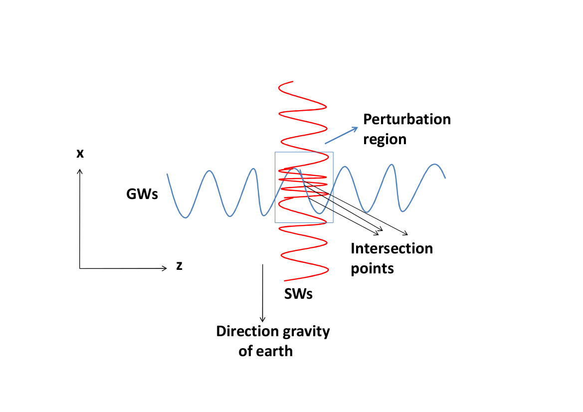
Figure 2: Encounter of GWs with SWs. GWs cause perturbation in SWs. This perturbation appears in the intersection points (the intersection point stands for the particle).

Now, as we propose this new experiment for the GWs detection as being not alternative but instead, complementary to interferometric GWs detectors. We use Eq. (23) to investigate about the possible detection of GWs from potential astrophysical and cosmological sources outside the frequency range where interferometers have the highest sensitivity, which is about $1Hz\leq f\leq 100Hz$ 5 ; 6 . A suitable range is one of the rotating NSs which till now have not yet been detected by LIGO. This is in the range of $100Hz\leq f\leq 1000Hz$ 5 ; 6 . In that case, any bumps on imperfections in the NS spherical shape generate GWs as the NS spins 5 . If the NS spin rate stays constant, so it emits the GWs 5 . Hence GWs are continuously with the same frequency and amplitude. Thus these are called “Continuous GWs”5 . The simplest model of the NS Continuous GWs emission is given by the so-called rigidly-rotating aligned triaxial ellipsoid a2 . The corresponding GW amplitude depends on the moments of inertia along three principal axes of the ellipsoid, which characterize the NS ellipticity, the distance to the source and the NS period of rotation a2 . An estimated upper bound is $h_{0+}\approx 10^{-24}$ a2 . The most rapidly rotating NSs currently known rotate at order of hundreds Hz 5 ; 6 . Considering an integration time of order of years and recalling that for the air it is $\rho_{0}\gamma^{2}\approx 10^{5}\,Pa$, while $-1\leq\sin kz\leq 1$, from Eq. (23) one gets

$$-10^{-9}\leq\Delta p_{NSs}\leq 10^{-9}\,Pa.$$ (24)

This seems a very small value, but for water we have instead $\rho_{0}\gamma^{2}\approx 10^{9}\,Pa$, which gives

$$-10^{-5}\leq\Delta p_{NSs}\leq 10^{-5}\,Pa.$$ (25)

The different results for another fluids are write down in Tab.1. The obtained amounts are more higher than corresponds amplitude of mentioned NS above $h_{0+}\approx 10^{-24}$. This seems to be an advantage with respect to standard interferometer technology.

Table.1. Variation of pressure due to the NSs and relic GWs in different fluids. Note that the symbol C means centigrade.
Matter $\rho_{0}\gamma^{2}$ $\;\;\Delta p_{NSs}$ $\Delta p_{relic\;GWs}$ Water $10^{9}$   $-10^{-5}\leq\Delta p\leq 10^{-5}$ $-10^{-8}\leq\Delta p\leq 10^{-8}$ Air $10^{5}$ $-10^{-9}\leq\Delta p\leq 10^{-9}$ $-10^{-12}\leq\Delta p\leq 10^{-12}$ Oil $10^{9}$ $-10^{-5}\leq\Delta p\leq 10^{-5}$ $-10^{-8}\leq\Delta p\leq 10^{-8}$ Acetic  acid $10^{9}$ $-10^{-5}\leq\Delta p\leq 10^{-5}$ $-10^{-8}\leq\Delta p\leq 10^{-8}$ Mercury $10^{10}$ $-10^{-4}\leq\Delta p\leq 10^{-4}$ $-10^{-7}\leq\Delta p\leq 10^{-7}$ Oxygen (-220 C) $10^{6}$ $-10^{-8}\leq\Delta p\leq 10^{-8}$ $-10^{-11}\leq\Delta p\leq 10^{-11}$ Molten  lead (340 C) $10^{10}$ $-10^{-4}\leq\Delta p\leq 10^{-4}$ $-10^{-7}\leq\Delta p\leq 10^{-7}$ Ether $10^{8}$ $-10^{-6}\leq\Delta p\leq 10^{-6}$ $-10^{-9}\leq\Delta p\leq 10^{-9}$ Ethanol $10^{9}$ $-10^{-5}\leq\Delta p\leq 10^{-5}$ $-10^{-8}\leq\Delta p\leq 10^{-8}$ Castor  oil $10^{9}$ $-10^{-5}\leq\Delta p\leq 10^{-5}$ $-10^{-8}\leq\Delta p\leq 10^{-8}$

The most important cosmological GWs source is given by the relic GWs. The production of relic GWs is well known in various works in the literature by using the so called adiabatically-amplified zero-point fluctuations process, which has been originally developed in the relic GWs framework by the soviet physicists L. P. Grishchuk a3 . Then, it has been shown how the standard inflationary scenario for the early universe can, in principle provide a distinctive spectrum of relic GWs a4 . The potential existence of relic gravitational radiation arises from general assumptions. It indeed derives from a mixing between basic principles of classical theories of gravity, starting from general relativity, and of quantum field theory. The zero-point quantum oscillations, which produce relic GWs, are generated by strong variations of the gravitational field in the early universe a3 ; a4 . Then, the detection of relic GWs is the only way to learn about the evolution of the very early universe, up to the bounds of the Planck epoch and the initial singularity a3 ; a4 . In more recent years, the analysis has been adapted also to the framework of extended theories of gravity a5 . In the standard inflationary scenario, the relic GWs are characterized by a dimensionless spectrum a4 ; a5

$$\Omega_{gw}(f)\equiv\frac{1}{\rho_{c}}\frac{d\rho_{gw}}{d\ln f},$$ (26)

where

$$\rho_{c}\equiv\frac{3}{8}H_{0}^{2}$$ (27)

is the critical energy density of the universe, $H_{0}$ the value of the Hubble expansion rate and $d\rho_{gw}$ the energy density of relic GWs in the frequency range $f$ to $f+df$. The spectrum of relic GWs in inflationary models is flat over a wide range of frequencies, that is in the range a4 -a5

$$10^{-16}Hz\leq f\leq 10^{10}Hz,$$ (28)

see fig.[3].

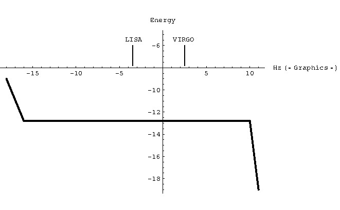
Figure 3: Adapted from ref. a5 . The spectrum of relic GWs in inflationary models is flat over a wide range of frequencies. The horizontal axis is $\log_{10}$ of frequency, in Hz. The vertical axis is $\log_{10}\Omega_{gw}$. The amplitude of the flat region depends only on the energy density during the inflationary stage; we have chosen the largest amplitude consistent with the WMAP constrains on scalar perturbations. This means that in the range $10^{-16}Hz\leq f\leq 10^{10}Hz$ it is $\Omega_{gw}(f)h_{100}^{2}\leq 9*10^{-13}$.

The spectrum is also connected with the characteristic amplitude $h_{C}$ of the relic GWs by the equation a4 ; a5

$$h_{C}(f)\simeq 1.26*10^{-18}\left(\frac{1{\rm Hz}}{f}\right)\sqrt{h_{100}^{2}\Omega_{gw}(f)}.$$ (29)

A dimensionless factor $h_{100}$ is included. It comes from an uncertainty in the value of $H_{0}$. In fact, for about 50 years in last century, $H_{0}$ was estimated to be between 50 and 90 (km/s)/Mpc generating a long controversy h1 . Such a controversy was partially resolved in the late 1990s through very precise cosmological observations due to the development of the Lambda-CDM model. Thus, the value of $h_{100}$ was fixed around 70 (km/s)/Mpc h2 . On the other hand, a more recent controversy (Hubble tension) started from difference between the estimations on the current value of $H_{0}$ calculated using CMB ($H_{CMB}=67.66\pm 0.42\ \textmd{Km/s/Mpc}$) cmb and SNeIa ($H_{SN}=74.03\pm 1.42\ \textmd{Km/s/Mpc}$) SNeIa .

In the range (28) it is a4 ; a5

$$\Omega_{gw}(f)h_{100}^{2}\leq 9*10^{-13},$$ (30)

which permits to write

$$h_{C}(f)\leq 10^{-24}\left(\frac{1{\rm Hz}}{\omega}\right)$$ (31)

in the same range. By combining Eqs. (23) and (31) and considering again an integration time of order of years one gets for the water

$$-10^{-8}\leq\Delta p_{relic\;GWs}\leq 10^{-8}\,Pa.$$ (32)

On the other hand, one can consider fluids different from water in order to obtain a series of results similar to Eqs. (25, 32). Such results due to NSs and relic GWs are written down in the Tab.1 for comparison purpose. The more suitable fluids seems to be the Mercury and Molten Lead (340 C). Therefore again our obtained results are higher than the strain based on standard interferometer technology ($h_{0+}\approx 10^{-24}$ as a sample) and has an advantage with respect to it.

Table.2. Variation of pressure due to GWs from different pulsars listed in a1 in different fluids.
Matter $\rho_{0}\gamma^{2}$ $\;\;\Delta p_{pulsar}(J0034-0534)$  $\Delta p_{pulsar}(J1301+0833)$ Water $10^{9}$   $-10^{-8}\leq\Delta p\leq 10^{-8}$ $-10^{-8}\leq\Delta p\leq 10^{-8}$ Air $10^{5}$ $-10^{-12}\leq\Delta p\leq 10^{-12}$ $-10^{-12}\leq\Delta p\leq 10^{-12}$ Oil $10^{9}$ $-10^{-8}\leq\Delta p\leq 10^{-8}$ $-10^{-8}\leq\Delta p\leq 10^{-8}$ Acetic  acid $10^{9}$ $-10^{-8}\leq\Delta p\leq 10^{-8}$ $-10^{-8}\leq\Delta p\leq 10^{-8}$ Mercury $10^{10}$ $-10^{-7}\leq\Delta p\leq 10^{-7}$ $-10^{-7}\leq\Delta p\leq 10^{-7}$ Oxygen (-220 C) $10^{6}$ $-10^{-11}\leq\Delta p\leq 10^{-11}$ $-10^{-11}\leq\Delta p\leq 10^{-11}$ Molten  lead (340 C) $10^{10}$ $-10^{-7}\leq\Delta p\leq 10^{-7}$ $-10^{-7}\leq\Delta p\leq 10^{-7}$ Ether $10^{8}$ $-10^{-9}\leq\Delta p\leq 10^{-9}$ $-10^{-9}\leq\Delta p\leq 10^{-9}$ Ethanol $10^{9}$ $-10^{-8}\leq\Delta p\leq 10^{-8}$ $-10^{-8}\leq\Delta p\leq 10^{-8}$ Castor  oil $10^{9}$ $-10^{-8}\leq\Delta p\leq 10^{-8}$ $-10^{-8}\leq\Delta p\leq 10^{-8}$

Table.3. Continued Tab.2
$\Delta p_{pulsar}(J1747-4036)$ $\Delta p_{pulsar}(J1902-5105)$ $\;\;\Delta p_{pulsar}(J1939+2134)$  $\Delta p_{pulsar}(J1959+2048)$ $-10^{-9}\leq\Delta p\leq 10^{-9}$ $-10^{-8}\leq\Delta p\leq 10^{-8}$   $-10^{-8}\leq\Delta p\leq 10^{-8}$ $-10^{-8}\leq\Delta p\leq 10^{-8}$ $-10^{-13}\leq\Delta p\leq 10^{-13}$ $-10^{-12}\leq\Delta p\leq 10^{-12}$ $-10^{-12}\leq\Delta p\leq 10^{-12}$ $-10^{-12}\leq\Delta p\leq 10^{-12}$ $-10^{-9}\leq\Delta p\leq 10^{-9}$ $-10^{-8}\leq\Delta p\leq 10^{-8}$ $-10^{-8}\leq\Delta p\leq 10^{-8}$ $-10^{-8}\leq\Delta p\leq 10^{-8}$ $-10^{-9}\leq\Delta p\leq 10^{-9}$ $-10^{-8}\leq\Delta p\leq 10^{-8}$ $-10^{-8}\leq\Delta p\leq 10^{-8}$ $-10^{-8}\leq\Delta p\leq 10^{-8}$ $-10^{-8}\leq\Delta p\leq 10^{-8}$ $-10^{-7}\leq\Delta p\leq 10^{-7}$ $-10^{-7}\leq\Delta p\leq 10^{-7}$ $-10^{-7}\leq\Delta p\leq 10^{-7}$ $-10^{-12}\leq\Delta p\leq 10^{-12}$ $-10^{-11}\leq\Delta p\leq 10^{-11}$ $-10^{-11}\leq\Delta p\leq 10^{-11}$ $-10^{-11}\leq\Delta p\leq 10^{-11}$ $-10^{-8}\leq\Delta p\leq 10^{-8}$ $-10^{-7}\leq\Delta p\leq 10^{-7}$ $-10^{-7}\leq\Delta p\leq 10^{-7}$ $-10^{-7}\leq\Delta p\leq 10^{-7}$ $-10^{-10}\leq\Delta p\leq 10^{-10}$ $-10^{-9}\leq\Delta p\leq 10^{-9}$ $-10^{-9}\leq\Delta p\leq 10^{-9}$ $-10^{-9}\leq\Delta p\leq 10^{-9}$ $-10^{-9}\leq\Delta p\leq 10^{-9}$ $-10^{-8}\leq\Delta p\leq 10^{-8}$ $-10^{-8}\leq\Delta p\leq 10^{-8}$ $-10^{-8}\leq\Delta p\leq 10^{-8}$ $-10^{-9}\leq\Delta p\leq 10^{-9}$ $-10^{-8}\leq\Delta p\leq 10^{-8}$ $-10^{-8}\leq\Delta p\leq 10^{-8}$ $-10^{-8}\leq\Delta p\leq 10^{-8}$

For the sake of completeness, we signal an important previous work a1 on an approach similar to the approach in this paper. The Authors of a1 analysed the sensitivity to continuous-wave strain fields of a kg-scale optomechanical system formed by the acoustic motion of super fluid helium-4 parametrically coupled to a superconducting microwave cavity. Such a narrow-band detection scheme can operate at very high Q-factors, while the resonant frequency is tunable through pressurization of the helium in the $0.1-1.5$ kHz range. Consequently, this kind of detector can, in principle, be tuned to a variety of astrophysical sources and also remain sensitive to a particular source over a long period of time. For thermal noise limited sensitivity, strain fields on the order of $h\simeq\frac{10^{-23}}{\sqrt{Hz}}$ could be, remarkably, detectable a1 . Therefore, the detector can compete with interferometric GWs detectors in particular for certain pulsar sources within a few months of integration time. Hence in next step and for comparison purpose, we select some of strains of different pulsars that called spin-down from Tab.1 of a1 to obtain a series of results from Eq. (23). A confrontation of Tab.1 of a1 with the our obtained numbers in Tab.2 shows an improvement of the sensitivity with respect to a1 . It seems indeed that the sensitivity arising from the method proposed in this work could be, in principle, higher than the sensitivity arising from the method proposed in a1 . This seems again to be an advantage with respect to standard interferometer technology and mentioned above method.

IV Noise in gravitational waves detectors

There are multiple sources of noise which can affect the performance of GWs detections. The more important types of noise in interferometers are thermal noise, shot noise, seismic noise and radiation pressure noise. The source of thermal noise arises from three main areas, that are the pendulum modes of suspension of the mirrors, the internal modes of the mirrors and the violin modes in the suspension wires. The shot noise arises from the quantum mechanical fluctuations in the phase quadrature of the electromagnetic field. The seismic noise comes from a lack of complete isolation of the mirrors form seismic activity. Finally, the radiation pressure noise arises from the quantum mechanical fluctuations in the amplitude quadrature of the electromagnetic field.

On the other hand, the detector which is suggested in this paper is different from the interferometer. The device that we propose, represents a variant what is referred to as a “resonant bar” detector, or“Weber bar”, after the scientist Joseph Weber pioneered their use a8 , with the important difference that it uses fluid as the medium instead of a solid such as aluminium or steel, as has been used traditionally a8 . The disadvantage of the fluid will likely have over another medium could be dissipation. Maybe the fluid will loose energy due to internal heating at too high a rate to be useful in building up a significant response to a GW. In fact, the aluminium resonant bar detectors have relied on the very high $Q$ factor of the material to absorb and store vibrational energy, building up a large response to a GW having the correct frequency. Therefore, one must take this into consideration when computing the sensitivity of the device. On the other hand, a recent approach in a9 could in principle permit to solve this problem. A new concept to drastically reduce acoustic radiation damping for fluids has been developed in a9 . A specifically designed cavity enclosing the resonator seems able to couple the radiated field back in the resonator a9 . Experiments on a custom tuning fork have been carried out and by realizing a cavity tenfold having a quality factor $Q=75.000$ in air at atmospheric pressure a9 . As the order of magnitude of $Q$ factors for aluminium are $1000<Q<10000$ a10 , i.e. one order of magnitude less than the one of the designed cavity in a10 . One hopes that the dissipation problem in fluids can be solved in the future.

Another noise that must be taken in account is thermal noise. In fact, at the scales being discussed in this paper, objects that we as humans perceive to be solid and stationary are neither a8 . At this scale, objects are composed of atoms, each of which is mechanically excited by thermal energy, and this cannot be ignored a8 . Robert Brown indeed detected in 1828 the “brownian motion” observing small particles of dust suspended in water a11 . Historically, the most remarkable physical interpretation of the “brownian motion” arises from a very famous paper of Albert Einstein a12 .

Seismic noise also cannot be ignored. One of the main sources of noise in this type of detector is indeed the gravity of the Earth. Hence, the detector must be supported somehow. A proposal in this sense could be to float it in space.

Thus, it is important to understand what is the order of magnitudes of different noises in order to see if they are comparable with respect to pressure changes coming from GWs. In fact, if the pressure changes due to GWs are smaller than those of noises, then using the experiment proposed in this paper will be impossible. By considering Tables 2 and 3, one sees that mercury seems to be the most suitable fluid to be used. In fact,for mercury the order of magnitude of pressure changes coming from GWs is $10^{-7}$. We recall that, in standard conditions for temperature and pressure, mercury is a very stable liquid largely used in thermometers, barometers, manometers. In particular and remarkably, in standard conditions for temperature and pressure, the pressure changes of mercury can be reduced to the order of magnitude of $10^{-8}$ 49 . This is due to mercury’s strong surface tension, high density and quasi-incompressibility49 . Thus, it seems that the using of mercury could permit, in principle, to detect GWs via the proposed experiment.

Finally, for the sake of completeness, it is important to stress the following:

Generally, in order to reduce noise:

1) One could reduce measuring bandwidth and i.e. to measure more slowly.

2) E.g. In order to obtain low-frequency AC measurements, then the current should be of low bias. That means that one should use primarily very low levels of signals. On the contrary, shot-noise is caused by the fluctuations in the number of photons detected at the photodiode. Consequently, this noise is minimized when utilizing a large laser power. Of course, these two cases conclude to diametrically opposed results relevant to avoiding shot noise, but their common characteristic is to use outlier conditions in the signal’s levels depending on the type of case.

3) Also, the only ways to reduce the thermal noise content are to reduce the temperature of operation.

4) Relevant to confronting the matter of seismic noise one could use the ”Seismic noise-reduction techniques for use with vertical stacking: An empirical comparison” thus the ”Possible earthquake forecasting in a narrow space-time-magnitude window”.

5) Relevant to ”radiation pressure noise”, and taking into consideration the Advanced LIGO interferometers, the quantum radiation pressure noise would be enhanced in the astrophysically important band of [10, 30] Hz, so the injection of squeezed states decreasing the shot noise would degrade the interferometers’ low-frequency sensitivity, see PT .

The suggested approaches to reduce noise could be the object of future works.

V Discussion and conclusion

In this paper a new experiment for the GWs detection has been proposed. The proposal is based on the investigation of the perturbation in a fluid. If GWs cross the fluid, they cause a perturbation in the shape of SWs in the fluid. This perturbation makes extra pressure and variations of the position, the velocity and the acceleration of the particles in the fluid. Thus GWs can be in principle, detected by carefully measuring these effects. This seems to be an advantage with respect to standard interferometer technology and another methods such as a1 , because one measures much higher quantities with respect to the very small strains due to GWs.

On the other hand, this proposed procedure may be difficult in practical experiments because of the presence of different types of noise. For this reason, a section of the paper has been dedicated to the discussion of such noises. We also stress that this paper must be considered as being pioneering in the new proposed approach. Thus one hopes that in future, more precise studies of the noise which concerns the proposed new experiment will be done.

VI Acknowledgements

The Authors thank the Referees for very useful comments and suggestions.

Appendix A

When the surface of wave moves in direction of x axis, the surfaces of molecules of neighbour fluid and parallel with surface of wave, vary their positions from the equilibrium state see Figure. (1). In general these variation of positions for the points on the each surface are equal to each other, function of two variables x (position) and t (time). We can show the variation with function $w(x,t)$. One can obtain relation between $w(x,t)$, density and pressure of fluid. We consider a layer of vertical section S that is between the two parallel surfaces in positions $x$ and $x+dx$ in equilibrium state. The mass of this layer is $\rho_{0}Sdx$. Now consider this layer moves to the $w,\,w+\frac{\partial w}{\partial x}dx$ due to right - pass wave (GWs in this work), see Figure 1. Then the new volume of layer will vary to $Sdx\left(1+\frac{\partial w}{\partial x}\right)$. The new volume generates a variation of the density while its mass remains constant. Thus, by assuming the mass conservation, one writes down

$$\rho Sdx\left(1+\frac{\partial w}{\partial x}\right)=\rho_{0}Sdx.$$ (33)

Setting $s\equiv\left(\frac{\rho-\rho_{0}}{\rho_{0}}\right),$ the above equation becomes

$$(1+s)\left(1+\frac{\partial w}{\partial x}\right)=1.$$ (34)

As it is $s\approx\frac{\partial w}{\partial x}\approx 10^{-4},$ the product $s\frac{\partial w}{\partial x}$ can be neglect in Eq. (34) and one gets

$$s=-\frac{\partial w}{\partial x}.$$ (35)

For the sake of simplicity, one considers a perfect fluid with $P=P(\rho)$ during an adiabatic process. Then

$$dP=\left(\frac{\partial P}{\partial\rho}\right)_{0}d\rho\quad with\quad d\rho=\rho-\rho_{0}.$$ (36)

Setting $p\equiv dP$ and considering the speed of propagation of the wave $\gamma$ given by $\gamma^{2}=\left(\frac{\partial P}{\partial\rho}\right)_{0},$ one gets

$$p=\rho_{0}\gamma^{2}s.$$ (37)

Thus, combining Eqs. (35) and (37) one obtains

$$p=-\rho_{0}\gamma^{2}\frac{\partial w}{\partial x}.$$ (38)

References

- (1) R. A. Hulse and J.H. Taylor, Astrophys. J. 195, L51 (1975).
- (2) J. L. Cervantes-Cota, S. Galindo-Uribarri e G. F. Smoot, Universe, 2(3), 22 (2016).
- (3) B. Abbott et al. (LIGO Scientific Collaboration and Virgo Collaboration), Phys. Rev. Lett. 116, 061102 (2016).
- (4) A. Einstein, Sitzungsber. K. Preuss. Akad. Wiss. 1, 688 (1916).
- (5) https://www.gw-openscience.org/catalog/
- (6) http://www.ligo.caltech.edu/advLIGO/
- (7) A. Freise (Virgo Collaboration), Class. Quant. Grav. 22, S 869 (2005).
- (8) H. Luck et al., Class. Quant. Grav. 14, 1471 (1997).
- (9) H. Takahashi, H. Tagoshi, amd (TAMA Collaboration), Class. Quant. Grav. 21, S 697 (2004).
- (10) http://tamago.mtk.nao.ac.jp/decigo/index_E.html
- (11) A. C. Searle, S.M. Scott, D. E. McClelland and L. S.Finn, Phys. Rev. D 73, 124014 (2006).
- (12) https://lisa.nasa.gov/
- (13) https://www.elisascience.org/
- (14) P. Amaro-Seoane et al., Class. Quant. Grav. 29, 124016 (2012).
- (15) C. Corda, Int. Journ. Mod. Phys. D 18, 2275 (2009).
- (16) C. Corda, Int. Journ. Mod. Phys. D 27, 1850060 (2018).
- (17) P. A. R. Ade et al. (BICEP2 Collaboration), Phys. Rev. Lett. 112, 241101 (2014).
- (18) R. Adam et al. (The Planck Collaboration) A&A 586, A133 (2016).
- (19) A. M. Cruise and R. M. J. Ingley, Class. Quant. Grav. 23, 6185 (2006).
- (20) M. L. Tong and Y. Zhang, Chin. J. Astron. Astrophys. 8, 3, 314 (2008).
- (21) F. Y. Li, M. X. Tang, J. Luo, and Y. C. Li, Phys. Rev. D 62, 044018 (2000).
- (22) F. Y. Li, M. X. Tang and D. P. Shi, Phys. Rev. D 67, 104008 (2003).
- (23) S. Singh et al., New J. Phys. 19, 073023 (2017).
- (24) Lawrence E. Kinsler et al, Fundamentals of Acoustics, 3rd Edition, ISBN:10: 0471094102, Wiley (1982).
- (25) C. W. Misner, K. S. Thorne and J. A. Wheeler, Gravitation, W. H. Feeman and Company (1973).
- (26) L. Landau and E. Lifsits, Classical Theory of Fields (3rd ed.), London: Pergamon (1971).
- (27) B. Abbott et al. (LIGO Scientific Collaboration and Virgo Collaboration), Phys. Rev. Lett. 116, 241103 (2016).
- (28) B. Abbott et al. (LIGO Scientific Collaboration and Virgo Collaboration), Phys. Rev. Lett. 118, 221101 (2017).
- (29) B. Abbott et al. (LIGO Scientific Collaboration and Virgo Collaboration), Phys. Rev. Lett. 119, 141101 (2017).
- (30) B. Abbott et al. (LIGO Scientific Collaboration and Virgo Collaboration), Phys. Rev. Lett. 119, 161101 (2017).
- (31) B. Abbott et al. (LIGO Scientific Collaboration and Virgo Collaboration), arXiv:1711.05578 (2017).
- (32) M. Sieniawska and M. Bejger, https://arxiv.org/abs/1909.12600.
- (33) L. P. Grishchuk, Zh. Eksp. Teor. Fiz. 67, 825 (1974).
- (34) B. Allen, Phys. Rev. D 37, 2078 (1988).
- (35) B. Ghayour and P. K. Suresh, Class. Quantum Grav. 29, 175009 (2012).
- (36) B. Ghayour and J. Khodagholizadeh, Eur. Phys. J. C 77, 560 (2017)
- (37) C. Corda, Eur. Phys. J. C 65, 257 (2010).
- (38) D.Overbye, ”Prologue”. Lonely Hearts of the Cosmos (2nd ed.). HarperCollins (1999).
- (39) P. A. R. Ade et al. (Planck Collaboration), Astron. Astrophys. 571, A16 (2014).
- (40) N. Aghanim, et al., (Planck Collaboration), Astron. Astrophys. 641, A6 (2020).
- (41) A. G. Riess., S. Casertano, W. Yuan, L. M. Macri, D. Scolnic, Astrophys. J. 876, 85 (2019).
- (42) A. Giazzotto, Jour. Phys. Conf. Ser. 120 (2008).
- (43) G. Aoust, R. Levy, B. Verlhac and O. Le Traon, Sens. Act. A: Phys. 269, 569 (2018)
- (44) W. Duffy Jr., Jour. Appl. Phys. 68, 5601 (1990)
- (45) R. Brown, Philos. Mag. 4 (21), 161 (1828)
- (46) A. Einstein, Ann. Phys. (in German) 322(8), 549 (1905).
- (47) S. Dwyer, Phys. Tod. 67, 11, 72 (2014).
- (48) E. R. Cohen et al. Quantities, Units and Symbols in Physical Chemistry, 3rd ed. Royal Society of Chemistry (2007).