Intermediate-luminosity red transients: Spectrophotometric properties and connection to electron-capture supernova explosions

We present the spectroscopic and photometric study of five intermediate-luminosity red transients (ILRTs), namely AT 2010dn, AT 2012jc, AT 2013la, AT 2013lb, and AT 2018aes. They share common observational properties and belong to a family of objects similar to the prototypical ILRT SN 2008S. These events have a rise time that is less than 15 days and absolute peak magnitudes of between $-11.5$ and $-14.5$ mag. Their pseudo-bolometric light curves peak in the range $0.5$ - $9.0\times 10^{40}\leavevmode\nobreak\ \mathrm{erg\leavevmode\nobreak\ s}^{-1}$ and their total radiated energies are on the order of (0.3 - 3) $\times$ 10⁴⁷ erg. After maximum brightness, the light curves show a monotonic decline or a plateau, resembling those of faint supernovae IIL or IIP, respectively. At late phases, the light curves flatten, roughly following the slope of the ⁵⁶Co decay. If the late-time power source is indeed radioactive decay, these transients produce ⁵⁶Ni masses on the order of $10^{-4}$ to $10^{-3}$ M_⊙ . The spectral energy distribution of our ILRT sample, extending from the optical to the mid-infrared (MIR) domain, reveals a clear IR excess soon after explosion and non-negligible MIR emission at very late phases. The spectra show prominent H lines in emission with a typical velocity of a few hundred km s^-1, along with Ca II features. In particular, the [Ca ii] $\lambda$7291,7324 doublet is visible at all times, which is a characteristic feature for this family of transients. The identified progenitor of SN 2008S, which is luminous in archival Spitzer MIR images, suggests an intermediate-mass precursor star embedded in a dusty cocoon. We propose the explosion of a super-asymptotic giant branch star forming an electron-capture supernova as a plausible explanation for these events.

1 Introduction

Modern surveys are discovering new types of stellar transients. Some events show intermediate luminosities lying between classical novae and core-collapse (CC) supernovae (SNe), and are collectively named ‘gap transients’ ($-$10 mag $<$M_V$<$ $-$15 mag; e.g. Kulkarni & Kasliwal 2009; Kasliwal 2012; Pastorello & Fraser 2019) or even intermediate-luminosity optical transients (e.g. Berger et al. 2009a; Soker & Kashi 2012; Soker 2020; Soker & Kaplan 2021).

A fraction of these transients are called ‘SN impostors’, as they mimic some observational properties of H-rich interacting SNe, but deep late-time imaging reveals that the progenitor stars survived (see, e.g. Van Dyk et al. 2000). Their typical peak absolute magnitudes are between $-13$ and $-15$ mag, and their spectra show narrow emission lines similar to Type IIn SNe (Schlegel, 1990; Filippenko, 1997). Giant eruptions of luminous blue variables (LBVs) are considered a plausible interpretation for classical SN impostors. During giant eruptions, their luminosity increases by over 3 mag with respect to the quiescent phase, accompanied by severe mass loss, sometimes exceeding 1 M_⊙  (Humphreys & Davidson, 1994; Humphreys et al., 1999). Well-studied examples are the historical giant eruptions of two Galactic LBVs: $\eta$ Carinae (e.g. Humphreys & Davidson, 1994; Soker, 2001a, b, 2003) and P Cygni (e.g. de Groot, 1969a, b), whose physical parameters (including ejected mass, spatial geometry, and radiated energy) have been well constrained.

Another class of gap transients has double-peaked light curves and fast-evolving spectra, showing SN IIn-like spectra at early phases (e.g. blue continuum and narrow H emission lines) and spectra similar to M-type stars at late phases (i.e. a much redder continuum and molecular bands). They are conventionally designated as luminous red novae (LRNe; e.g. see Kochanek et al., 2014; Pejcha et al., 2016; Smith et al., 2016; Blagorodnova et al., 2017; Lipunov et al., 2017; MacLeod et al., 2017; Pejcha et al., 2017; Cai et al., 2019; Pastorello et al., 2019a, b, 2021a, 2021b). The LRN phenomenon is usually interpreted as a post-common-envelope-ejection phase in a contact binary system, and may be followed by stellar coalescence (e.g. see Munari et al., 2002; Soker & Tylenda, 2003, 2006; Tylenda et al., 2011; Soker & Kashi, 2016; Smith et al., 2016; Lipunov et al., 2017; Mauerhan et al., 2018; Pastorello et al., 2019b; Soker, 2021).

The third group of gap transients are named intermediate-luminosity red transients (ILRTs; Pastorello & Fraser, 2019, and references therein). These show a slow rise time ($\approx$ 2 weeks) to maximum ($-$11.5 mag $<$M_V$<$ $-$14.5 mag), followed by a linear decline or a plateau lasting about 2-4 months. When late-time light curves are observed, they decline following the expectation of ⁵⁶Co decay. Their light curves resemble those of very faint SNe IIP/L. The spectra are similar to Type IIn SNe with narrow Balmer lines in emission, but are characterised by prominent Ca ii lines (e.g. Ca H&K, [Ca ii] doublet, and Ca ii near-infrared triplet); in particular, the [Ca ii] $\lambda\lambda$ 7291, 7324 doublet is always visible at all phases. ILRTs are linked to 8-15 M_⊙  progenitors and are strong mid-infrared (MIR) emitters, suggesting their progenitors are embedded in dusty cocoons (see Prieto et al., 2008; Bond et al., 2009; Botticella et al., 2009; Berger et al., 2009b; Thompson et al., 2009). However, their origin remains mysterious and different scenarios are contemplated. These transients have been proposed to be LBV-like outbursts of moderate-mass stars (e.g. Smith et al., 2009; Andrews et al., 2020) or stellar mergers (e.g. Kasliwal et al., 2011). A third suggested scenario is that we are actually observing faint CC SN explosions triggered by electron captures in the core of super-asymptotic giant branch (S-AGB) stars, and these are therefore labelled electron-capture (EC) SNe (see, e.g. Botticella et al., 2009; Pumo et al., 2009). In recent years, a number of ILRTs have been studied, including SN 2008S (see, e.g. Prieto et al., 2008; Botticella et al., 2009; Smith et al., 2009; Kochanek, 2011; Szczygieł et al., 2012; Adams et al., 2016), NGC 300-2008OT1 (NGC 300 OT hereafter) (e.g. Berger et al., 2009b; Bond et al., 2009; Prieto et al., 2009; Kashi et al., 2010; Humphreys et al., 2011), M85 OT2006-1 (Kulkarni et al., 2007; Pastorello et al., 2007; Rau et al., 2007), PTF10fqs (Kasliwal et al., 2011), AT 2017be (Stephens et al., 2017; Adams et al., 2018; Cai et al., 2018), and AT 2019abn (Jencson et al., 2019; Williams et al., 2020, Valerin et al. 2021, in preparation).

In this paper, we analyse a sample of five ILRTs , including AT 2010dn, AT 2012jc, AT 2013la, AT 2013lb, and AT 2018aes. In general, they were initially classified as LBV-like outbursts or, more generically, SN impostors. Subsequent follow-up campaigns allowed us to confirm their classifications as ILRTs. In this work, we also compared ILRTs with other claimed EC SN candidates, such as SN 2018zd (Zhang et al., 2018; Arcavi et al., 2018; Zhang et al., 2020; Hiramatsu et al., 2021; Kozyreva et al., 2021, Callis et al. 2021, in preparation), SN 2018hwm (Reguitti et al., 2021), and SN 2015bf (Lin et al., 2021), as well as underluminous SNe IIP (i.e. SN 1999br, SN 2005cs; Pastorello et al., 2004, 2006, 2009).

The present paper is organised as follows: general information on the sampled ILRTs is given in Sect. 2. Photometric and spectroscopic analysis is reported in Sects. 3 and 4, respectively. The rate of ILRTs is estimated in Sect. 5. Finally, a discussion on the observational and theoretical properties of ILRTs is given in Section 6.

2 Basic sample information

2.1 Host galaxies: distance, reddening and metallicity

AT 2010dn was discovered by the amateur astronomer K. Itagaki in May 2010 at 31.523 UT (hereafter UT will be used throughout this paper) at an unfiltered magnitude 17.5 mag (CBAT). The object was detected at RA=$10^{h}18^{m}19\aas@@fstack{s}89$, Dec=$+41\degr 26\arcmin 28\arcsec.80$ [J2000], $61\arcsec$ north and $33\arcsec$ east from the centre of NGC 3184. We adopt $d=14.40\pm 0.33$ Mpc ($\mu=30.79\pm 0.05$ $\mathrm{mag}$) as the distance to the host galaxy, as obtained from Cepheids (Ferrarese et al., 2000). The Galactic reddening $E(B-V)_{\mathrm{Gal}}=0.017$ $\mathrm{mag}$ is from Schlafly & Finkbeiner (2011). The presence of narrow interstellar Na I D ($\lambda\lambda$ 5890, 5896) absorption in the transient spectra at the host galaxy redshift is usually considered as evidence for additional internal extinction (e.g. Munari & Zwitter, 1997; Turatto et al., 2003; Pozzo et al., 2006; Sahu et al., 2006; Poznanski et al., 2011). In this case, the equivalent width (EW) of Na I D varies with time, suggesting that this dust is likely due to circumstellar material (CSM). For this reason, we neglect the possible host component of extinction and adopt a total reddening E($B-V$)_Total = E($B-V$)_Gal = 0.017 $\mathrm{mag}$, in agreement with Smith et al. (2011).

AT 2012jc (also known as PSN J14535395+0334049, NGC 5775-2012OT1, SNhunt120 and LSQ12brd) was found by S. Howerton and the Catalina Real-Time Transient Survey (CRTS) in March 2012 at 27.460 UT (Berger et al., 2012; Howerton et al., 2012). Its coordinates are: RA=$14^{h}53^{m}53\aas@@fstack{s}95$, Dec=$+03\degr 34\arcmin 04\arcsec.90$ [J2000], and it is located at $85\arcsec$ north and $55\arcsec$ west from the centre of NGC 5775. Based on the weighted average of several estimates using the Tully-Fisher method (e.g. Tully et al., 2013; Sorce et al., 2014; Tully et al., 2016) from the NASA/IPAC Extragalactic database (NED), a distance of $d=18.62\pm 1.12$ Mpc (hence $\mu=31.35\pm 0.13$ $\mathrm{mag}$) can be estimated for NGC 5775. A Galactic reddening E($B-V$)_Gal = 0.037 $\mathrm{mag}$ (Schlafly & Finkbeiner, 2011) is adopted. We measure a constant $EW\simeq 0.9$ Å for the Na i D absorption at the redshift of NGC 5775 in the early spectra of the transient. Following Turatto et al. (2003) and assuming R_V = 3.1 (Cardelli et al., 1989), we obtain a host galaxy reddening of $E(B-V)_{\mathrm{Host}}=0.144$ $\mathrm{mag}$. Hence, the total reddening towards AT 2012jc is $E(B-V)_{\mathrm{Total}}$ = 0.181 $\mathrm{mag}$.

The discovery of AT 2013lb (PSN J15213475-0722183; NGC 5917-2013OT1) was announced by the CHilean Automatic Supernovas sEarch in January 2013 at 27.340 UT (CHASE, Pignata et al., 2009; Margheim et al., 2013). The coordinates are RA=$15^{h}21^{m}34\aas@@fstack{s}75$, Dec=$-07\degr 22\arcmin 18\arcsec.30$ [J2000], and $19\arcsec$ north and $31\arcsec$ east from the centre of NGC 5917. For this galaxy, we adopt a kinematic distance, assuming a standard cosmological model with $H_{0}=73$ $\rm{km}\,s^{-1}$$\rm{Mpc}^{-1}$, $\Omega_{\mathrm{M}}=0.27$, $\Omega_{\mathrm{\Lambda}}=0.73$ (Spergel et al., 2007), which is used throughout this paper. From the radial velocity corrected for Local Group infall onto the Virgo Cluster $V_{\mathrm{Vir}}$ = 2024 $\pm$ 7 $\rm{km}\,s^{-1}$  (see Sandage & Tammann, 1990; Theureau et al., 1998; Terry et al., 2002, reported by HyperLeda ), we obtain a luminosity distance $d=27.73\pm 1.90$ Mpc ($\mu=32.21\pm 0.15$ $\mathrm{mag}$). A Galactic reddening $E(B-V)_{\mathrm{Gal}}=0.085$ $\mathrm{mag}$ (Schlafly & Finkbeiner, 2011) is reported for this object. Additionally, spectroscopy indicates a negligible host galaxy extinction based on non-detection of the Na i D absorption feature at the redshift of the host galaxy.

AT 2013la (also named PSN J13100734+3410514; PS1-14ln; UGC 8246-2013OT1) was discovered by B. Wang and X. Gao in December 2013 at 20.932 UT, at RA=$13^{h}10^{m}07\aas@@fstack{s}34$, Dec=$+34\degr 10\arcmin 51\arcsec 40$ [J2000] (e.g. Tartaglia et al., 2014). The object is $0.8\arcsec$ south and $32.7\arcsec$ east from the centre of UGC 8246. Averaging several recent Tully-Fisher estimates (e.g. Tully et al., 2013; Sorce et al., 2014; Tully et al., 2016), we obtain $d=15.21\pm 0.11$ Mpc (hence, $\mu=30.91\pm 0.02$ $\mathrm{mag}$) for UGC 8246. We adopt the same line-of-sight reddening as Barsukova et al. (2014), that is, $E(B-V)_{\mathrm{Total}}=0.009$ $\mathrm{mag}$. We note that, in analogy to AT 2010dn, a variable $EW$ of Na I D suggests the presence of additional circumstellar dust, which is not accounted for in this reddening estimate. We hence adopt $E(B-V)_{\mathrm{Total}}=E(B-V)_{\mathrm{Gal}}$.

AT 2018aes (Kait-18M) was discovered by the Lick Observatory Supernova Search (LOSS) in March 2018 at 11.535 (Yunus et al., 2018). It was detected at RA=$13^{h}48^{m}17\aas@@fstack{s}76$, Dec=$+03\degr 56\arcmin 44\arcsec.20$ [J2000], $18.9\arcsec$ south and $25.7\arcsec$ east of the nucleus of NGC 5300 (Andrews et al., 2018). We average a few recent Tully-Fisher distances estimates from NED (e.g. Tully et al., 2013; Sorce et al., 2014; Tully et al., 2016), obtaining a weighted average distance $d=18.02\pm 0.61$ Mpc ($\mu=31.28\pm 0.07$ $\mathrm{mag}$). As there is some persistent spectroscopic signatures of interstellar Na I D at the host galaxy redshift, following Turatto et al. (2003), we estimate an internal reddening $E(B-V)_{\mathrm{Host}}=0.160$ $\mathrm{mag}$, while we adopt a Milky Way contribution $E(B-V)_{\mathrm{Gal}}=0.020$ $\mathrm{mag}$ (Schlafly & Finkbeiner, 2011) for AT 2018aes. Hence, we obtain a total colour excess $E(B-V)_{\mathrm{Total}}=0.180$ $\mathrm{mag}$.

Although we did not perform precise estimates of metallicity at the locations of these ILRTs, an estimate of the characteristic oxygen abundance at $0.4R_{25}$ can be done using a statistical approach and the following relation from Pilyugin et al. (2004):

$$12+\mathrm{log}\left(\mathrm{O/H}\right)\leavevmode\nobreak\ $=$\leavevmode\nobreak\ 6.93\leavevmode\nobreak\ \left(\pm\leavevmode\nobreak\ 0.37\right)\leavevmode\nobreak\ -\leavevmode\nobreak\ 0.079\leavevmode\nobreak\ \left(\pm\leavevmode\nobreak\ 0.018\right)\leavevmode\nobreak\ \times\leavevmode\nobreak\ M_{\mathrm{B}},$$ (1)

which links the characteristic oxygen abundance to the absolute $B$-band magnitude ($M_{\mathrm{B}}$) of the galaxy. The oxygen abundances of the ILRT host galaxies span a very narrow range, from 8.2 to 8.6 $\mathrm{dex}$, which is nearly solar or marginally subsolar (adopting a solar metallicity of 12 + log(O/H) = 8.69 dex; see e.g. Asplund et al., 2009; von Steiger & Zurbuchen, 2016; Vagnozzi, 2019). We note that the hosts are all spiral galaxies and the positions of the ILRTs are towards their outer edges.

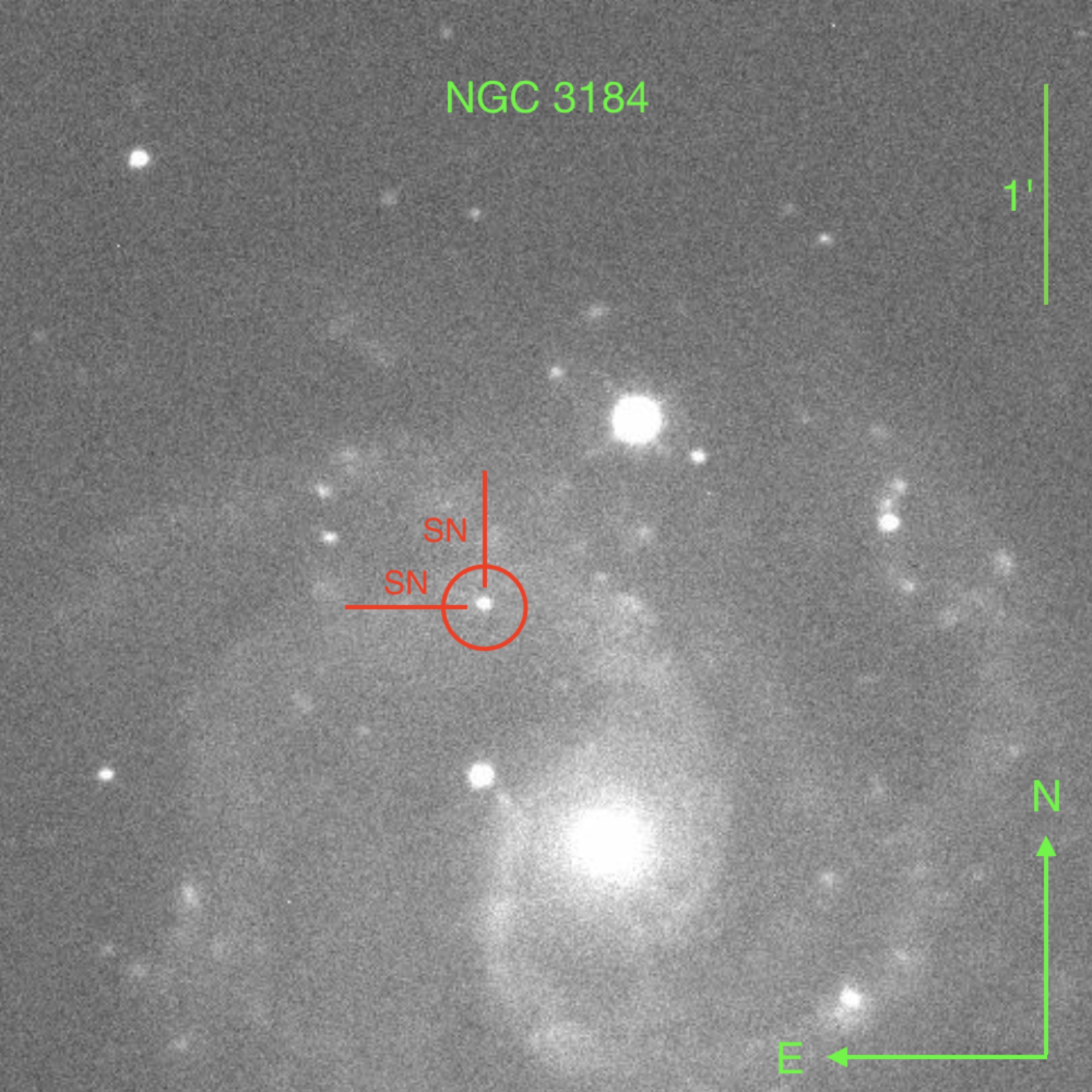
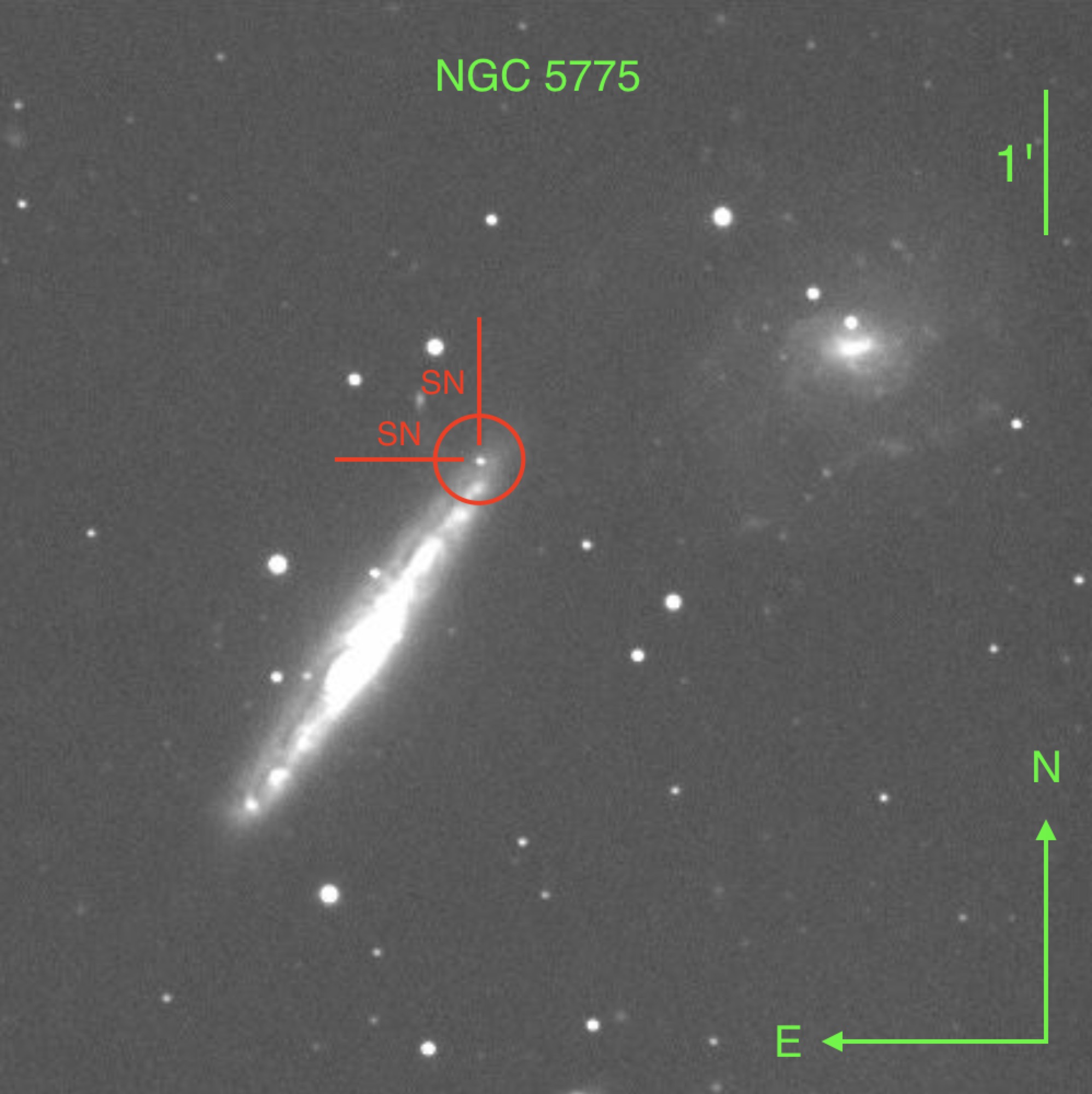
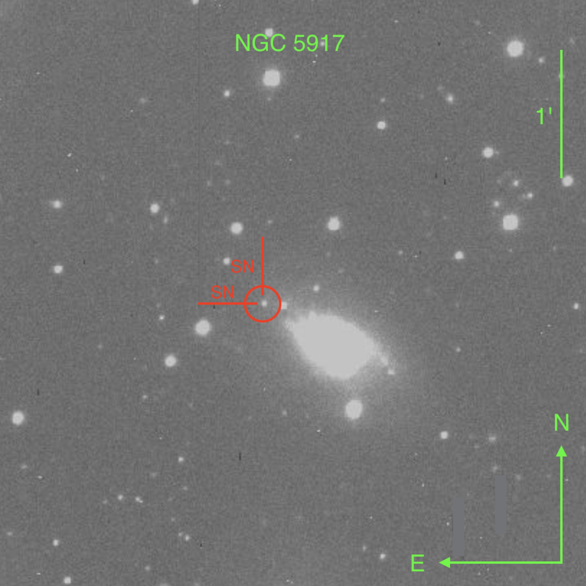
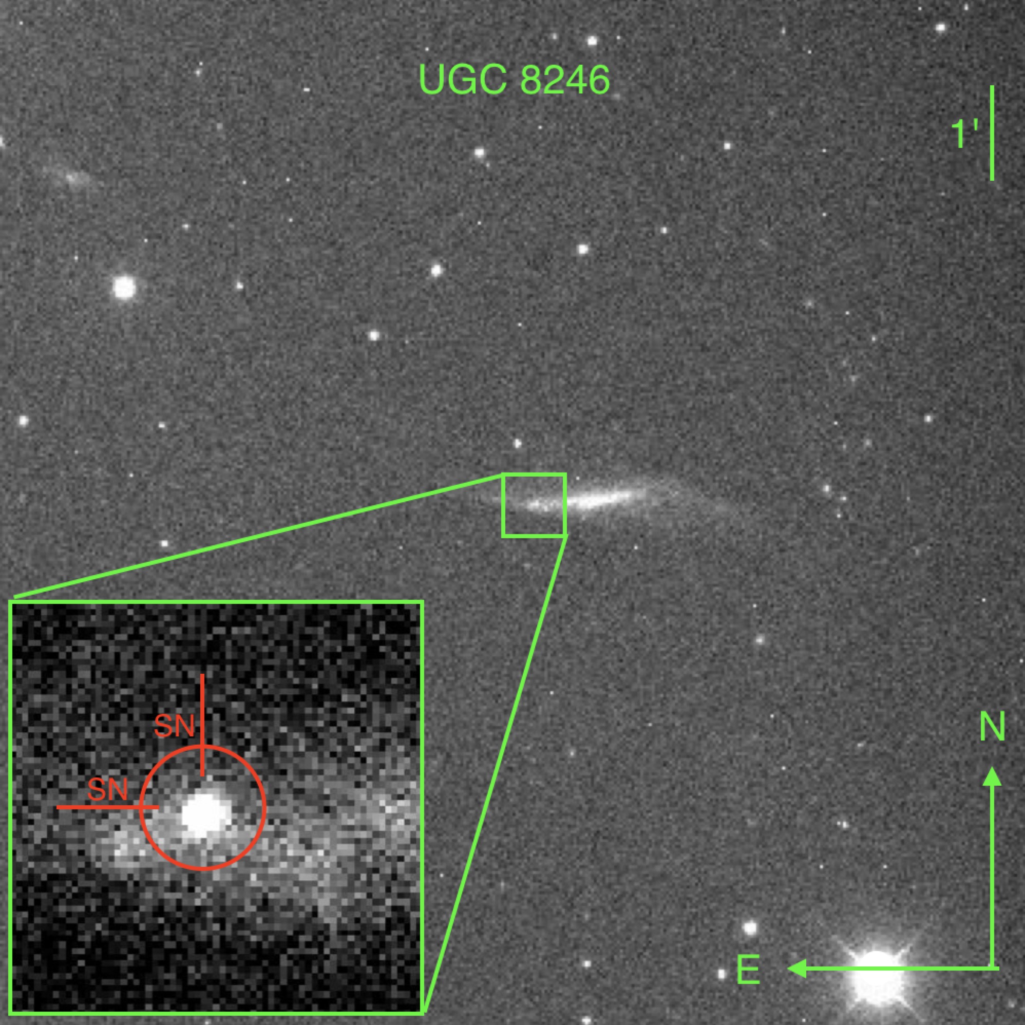
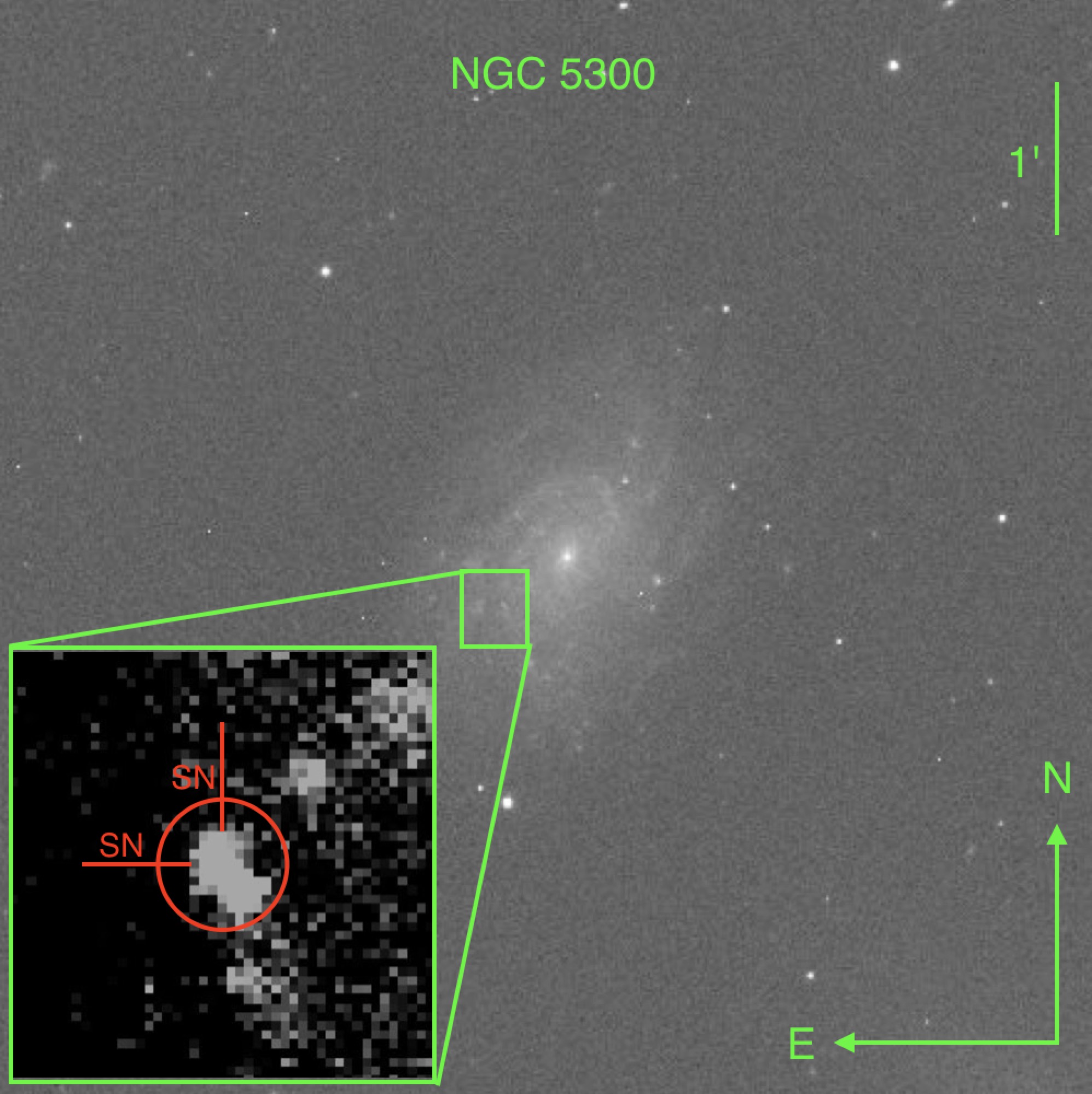
Figure 1: Top-left: AT 2010dn in one of the spiral arms of the host galaxy. Sloan $r$-band image taken in June 2010 at 19 with the 2m robotic Faulkes Telescope North (FTN) operated by Las Cumbres Observatory (LCO; Brown et al., 2013). Top-middle: AT 2012jc at the north edge of its host galaxy. Johnson-Cousins $R$-band image obtained in April 2012 at 06 with the 0.41m PROMPT5 telescope. Top-right: AT 2013lb in the outskirts of its host galaxy. Johnson-Cousins $R$-band image obtained in February 2013 at 20 with the 2m fully robotic Liverpool Telescope (LT) with RATCam. Bottom-left: AT 2013la at the east edge of its galaxy. A zoom-in of the transient position is shown in the lower-left corner. Sloan $r$-band image obtained in February 2014 at 12 with the LT equipped with IO:O. Bottom-right: AT 2018aes and its host galaxy. LT/IO:O Sloan $r$-band image obtained in May 2018 at 17 with a blow-up of the transient site in the lower-left inset.

A summary of the ILRTs and their host galaxy parameters is listed in Table 1, while in Figure 1 we show the location of the transients in their host galaxies.

Table 1: Basic information for the ILRT host galaxies.

Object	Host Galaxya	$m_{\mathrm{B}}$b	Redshift	Distance	Distance Modulus	Radial Distancec	Metallicity	$E(B-V)_{\mathrm{Gal}}$	$E(B-V)_{\mathrm{Host}}$
		($\mathrm{mag}$)		($\mathrm{Mpc}$)	($\mathrm{mag}$)	($\mathrm{kpc}$)	($\mathrm{dex}$)	($\mathrm{mag}$)	($\mathrm{mag}$)
AT 2010dn	NGC 3184 [SABc]	10.3	0.00198	14.40 (0.33)	30.79 (0.05)	4.8 (0.1)	8.55 (0.74)	0.017	0
AT 2012jc	NGC 5775 [SBc]	12.2	0.00561	18.62 (1.12)	31.35 (0.13)	9.1 (0.5)	8.44 (0.71)	0.037	0.144 (0.080)
AT 2013lb	NGC 5917 [Sb]	13.7	0.00635	27.73 (1.90)	32.21 (0.15)	2.7 (0.1)	8.39 (0.70)	0.085	0
AT 2013la	UGC 8246 [SBc]	14.6	0.00271	15.21 (0.11)	30.91 (0.02)	4.0 (0.3)	8.22 (0.66)	0.009	0
AT 2018aes	NGC 5300 [SABc]	12.1	0.00391	18.02 (0.61)	31.28 (0.07)	2.8 (0.1)	8.45 (0.72)	0.020	0.160 (0.085)
SN 2008S	NGC 6946 [SABc]	8.2	0.00013	5.70 (0.21)	28.78 (0.08)	5.6 (0.2)	8.56 (0.74)	0.360	0.320 (0.031)
NGC300 OT	NGC 0300 [Scd]	8.8	0.00048	1.88 (0.12)	26.37 (0.14)	2.5 (0.2)	8.32 (0.69)	0.011	0.250 (0.148)
PTF10fqs	NGC 4254 [Sc]	10.2	0.00803	14.26 (3.41)	30.77 (0.52)	6.9 (1.7)	8.56 (0.74)	0.040	0
AT 2017be	NGC 2537 [SBm]	13.1	0.00144	7.82 (0.54)	29.47 (0.15)	-	8.22 (0.66)	0.048	0.040 (0.02)
M85 OT	NGC 4382 [S0-a]	10.1	0.00243	15.85 (0.88)	31.00 (0.12)	2.5 ( 0.1)	8.58 (0.75)	0.027	0.113 (0.108)

$Notes:$ Our sample is reported in the top half of the table and other published objects are in the lower half. The uncertainties on distance, distance modulus, radial distance, and metallicity are obtained from error propagations, while host galaxy extinction is computed from the standard deviation of measurements.

^a Galaxy type from HyperLeda.

^b $B$-band apparent magnitude of the host galaxy, from NED.

^c Projected distance of the ILRT location from the host galaxy nucleus.

2.2 Data reduction

Routine follow-up campaigns were triggered soon after the announcement of the ILRT discoveries, using the instruments available to our collaboration. Information on the instrumental configurations is reported in Table 6 (Appendix A). For some transients, additional early-time unfiltered data were collected from amateur astronomers. We also collected historical data available in public archives.

The raw images were first pre-reduced, applying overscan, bias and flat-field corrections through standard iraf tasks (Tody, 1986, 1993). When necessary, multiple-exposure frames were median-combined to increase the signal-to-noise ratio (S/N). Photometric measurements were performed through a dedicated pipeline, ecsnoopy. ecsnoopy is a python-based script, which makes use of a series of packages for photometry and template subtraction (e.g. sextractor, daophot, hotpants; Bertin & Arnouts, 1996; Stetson, 1987; Becker, 2015). Individual instrumental magnitudes were measured with the point-spread function (PSF) fitting technique. We first subtracted the background contaminating the object using a low-order polynomial fit. A standard PSF template was constructed by fitting the profiles of several isolated stars (usually from 5 to 10 stars) in the SN frames. The PSF model was then fitted to the target source, and the goodness of the fit was evaluated by inspecting the residuals at the SN location. When the object was faint or had a complex background, we used the template-subtraction technique to remove the background contamination from our measurements. Specifically, we applied it to measurements of AT 2010dn, AT 2013la, and AT 2018aes. The errors were estimated via artificial star tests, in which several fake stars were placed close to the SN location. The fake stars were fitted with the PSF method, and the standard deviation of these measurements provided us the instrumental errors. These were combined in quadrature with the PSF-fit error, finally providing the total photometry error.

We applied the instrumental zero points (ZPs) and colour terms (CTs) to the instrumental magnitudes obtained through observations of standard fields obtained in photometric nights. Specifically, the Johnson-Cousins magnitudes were determined with reference to the Landolt (1992) catalogue, and Sloan-filter data were calibrated via the SDSS DR 13 catalogue (Albareti et al., 2017). In order to obtain an accurate calibration, a sequence of reference stars in the field of each ILRT was used to correct the ZPs in non-photometric nights. When available, the Sloan magnitudes of the reference stars in the ILRT field were directly taken from SDSS, while the Johnson-Cousins magnitudes were obtained from the SDSS data using the conversion relations of Chonis & Gaskell (2008).

Near-infrared (NIR) data reduction includes flat fielding, distortion correction and sky subtraction. We performed pre-reduction on NOT/NOTCam and NTT/SOFI raw images using dedicated pipelines for NOTCam (version 2.5) and SOFI (PESSTO pipeline, version 2.2.10; Smartt et al., 2015) respectively. Standard iraf tasks were used to reduce LT/SupIRCam and TNG/NICS images. Instrumental magnitudes were measured via ecsnoopy, and then calibrated using the Two Micron All Sky Survey (2MASS, Skrutskie et al., 2006) catalogue (assuming negligible colour corrections).

The Spitzer Space Telescope was equipped with the InfraRed Array Camera (IRAC; two channels: CH1=3.6 $\mu$m and CH2=4.5 $\mu$m). We used the Level 2 post-BCD (Basic Calibrated Data) images, which were reduced with the Spitzer pipeline. These pBCD images are composed of a mosaic image, after rejection of most instrumental artefacts, an uncertainty image, and an associated coverage image which is the map of how many frames per position are available to generate the mosaic image. We note that AT 2010dn was targeted at 14 epochs by the Spitzer Space Telescope during 2010 – 2015 and the data are available from Spitzer Heritage Archive (SHA). We took the Spitzer images from 2019 September 14 as templates, which were matched and transformed to each epoch of the observed images and then subtracted using hotpants (Becker, 2015). We performed aperture photometry on the subtracted images using a small (4$\times$$0.6\arcsec$ pBCD pixel) aperture, and then applied an aperture correction and a conversion from MJy/sr to mJy/pix to get the fluxes. With this approach, we obtained ten detections for the CH1 and CH2 channels over a time-span of five years (from 2010 to 2015). For a few other epochs we have non-detections down to 3$\sigma$. The resulting magnitudes are reported in Table 10 (Appendix C).

3 Photometry

Our follow-up campaigns for each of the five transients started soon after their discovery, and lasted several months. The photometric measurements of the transients are reported in Tables 8 - 17 (Appendix C), while individual light curves are shown in Figure 2. As a reference epoch, we selected the $R/r$-band maximum, obtained using a third-order polynomial fit to the observed light curves between about $-$20 and $+$20 days from maximum (see below).

3.1 Apparent light curves

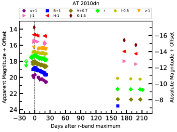
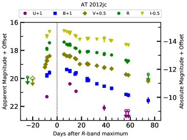
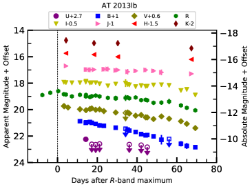
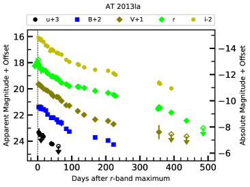
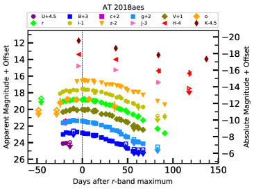
Figure 2: Multi-band light curves of AT 2010dn (top-left), AT 2012jc (top-right), AT 2013lb (middle-left), AT 2013la (middle-right), and AT 2018aes (bottom). The dashed vertical lines indicate the $R/r$-band maximum time. Upper limits are marked by empty symbols with arrows. The light curves are shifted with some constants for clarity and the shift amount is reported at the top. The errors of most magnitudes are smaller than the plotted symbol sizes.

Table 2: Decline rates of the light curves of individual ILRTs (mag/100d), along with their uncertainties.

Filter	Phase i ($\gamma$1)	Phase ii ($\gamma$2)	Phase iii ($\gamma$3)
AT 2010dn
$u$	6.32 (0.54)	4.25 (0.56)	–
$B$	6.23 (0.92)	4.02 (0.38)	–
$V$	6.36 (1.24)	2.14 (0.36)	0.08 (0.05)
$r$	5.17 (0.96)	1.50 (0.38)	0.08 (0.05)
$i$	6.16 (0.43)	1.03 (0.51)	0.29 (0.15)
$z$	0.89 (0.06)	0.89 (0.06)	–
$J$	1.45 (0.11)	1.45 (0.11)	1.41 (0.00)
$H$	0.72 (0.05)	0.72 (0.05)	0.80 (0.00)
$K$	–	–	1.75 (0.00)
AT 2012jc
$U$	5.78 (0.79)	5.78 (0.79)	–
$B$	4.16 (0.29)	2.77 (0.19)	2.77 (0.19)
$V$	3.17 (0.37)	2.20 (0.10)	2.20 (0.10)
$R$	4.98 (0.44)	-0.11 (0.35)	2.68 (0.27)
$I$	4.14 (0.44)	0.09 (0.20)	2.24 (0.08)
AT 2013lb
$B$	–	3.41 (0.09)	3.41 (0.09)
$V$	1.90 (0.12)	1.90 (0.12)	4.94 (0.52)
$R$	1.10 (0.11)	1.10 (0.11)	5.13 (0.18)
$I$	0.59 (0.10)	0.59 (0.10)	5.12 (1.35)
$J$	0.56 (0.10)	0.56 (0.10)	0.56 (0.10)
$H$	0.74 (0.10)	0.74 (0.10)	0.74 (0.10)
$K$	0.91 (0.12)	0.91 (0.12)	0.91 (0.12)
AT 2013la
$u$	2.22 (0.04)	2.22 (0.04)	–
$B$	2.08 (0.07)	0.71 (0.11)	–
$V$	1.79 (0.03)	0.59 (0.27)	–
$r$	1.70 (0.05)	0.62 (0.04)	1.17 (0.12)
$i$	1.72 (0.07)	0.37 (0.11)	1.14 (0.09)
AT 2018aes
$B$	2.21 (0.21)	3.78 (0.13)	5.02 (1.99)
$g$	1.85 (0.22)	4.02 (0.23)	4.97 (0.90)
$V$	2.25 (0.25)	4.33 (0.27)	5.01 (2.05)
$r$	2.55 (0.34)	3.75 (0.13)	6.51 (0.04)
$i$	2.17 (0.68)	4.03 (0.21)	4.48 (0.39)
$z$	2.52 (0.89)	3.72 (0.30)	5.02 (0.14)
$J$	2.32 (0.28)	2.32 (0.28)	2.32 (0.28)
$H$	2.01 (0.26)	2.01 (0.26)	2.01 (0.26)
$K$	1.57 (0.21)	1.57 (0.21)	1.57 (0.21)

In Figure 2 we show the apparent light curves of the five events, which are similar to those of other ILRTs in the literature. Most of the objects have a rise time of about two weeks, but AT 2018aes has a longer rise of about 24.1 d. After maximum, the light curve evolution of the sample resembles that of SNe IIP/IIL. We divide the light curve evolution into three different phases: Phase i ($\gamma$₁), Phase ii ($\gamma$₂), and Phase iii ($\gamma$₃), each with a different decline rate. The values obtained through linear fits are reported in Table 2. In general, ILRTs decline quite rapidly in all bands during Phase i, with the blue bands usually fading faster than the red bands. After Phase i, a sort of plateau (see AT 2012jc and AT 2013la) or a linear decline (see AT 2013lb and AT 2018aes) is observed in ILRTs. When late-time observations are available (i.e. AT 2013la, SN 2008S, and NGC 300 OT), a slow evolution is observed, consistent with that expected from the ⁵⁶Co decay. We discuss the implications of this in Sect. 3.4.

3.2 Colour evolution

The colour evolution of the five transients is shown in Figure LABEL:pic:colour, along with those of other ILRTs and comparison objects from the literature. For the ILRTs, the $B-V$ colour evolves steadily from $\sim$ 0.2 - 0.4 mag at early phases to $\sim 0.7$ - 1.0 mag at around 100 days past maximum, suggesting that the temperature decreases with time (see panel a in Figure LABEL:pic:colour). At the later phases ($>$100 days), $B-V$ becomes bluer again, from 0.8 to 0.5 mag. At similar epochs, the $R-I$/$r-i$ colours increase from $\sim$ 0.1 - 0.3 mag to 0.5 - 1.0 mag (Figure LABEL:pic:colour, panel b). Very late-time colours show a large dispersion. AT 2013la is somewhat discrepant, with the $r-i$ colour becoming bluer (reaching $\sim-0.2$ mag) than at early epochs. The $J-K$ colour usually shows a minimum at 30-70 days. The best-sampled NIR dataset is that of NGC 300 OT, which allows us to estimate a minimum value of $\sim$ 1.1 mag. Later, $J-K$ rises to 3.0 mag at $\sim$ 230 days (Figure LABEL:pic:colour, panel c). As shown in Figure LABEL:pic:colour, the comparison objects are bluer (e.g. SN 2018zd and SN 2005cs: $B-V$ $\approx$ $-$0.2 mag) at early phase and become redder (e.g. SN 2005cs: $B-V$ $\approx$ 2.0 mag at tail phase) over time.

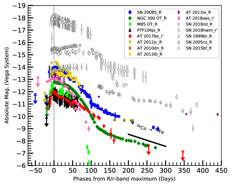
Figure 4: Comparison of the $R/r$-band absolute light curves of ILRTs and SN 2018zd, SN 2018hwm, SN 1999br, and SN 2005cs. Reddenings and distance moduli of the comparison objects are taken from their respective papers (also see Table 7 in Appendix B). The dashed vertical line indicates the time of $r$-band maximum light. Upper limits are marked by empty symbols with down arrows.

3.3 Absolute light curves

The $R/r$-band absolute light curves of our ILRT sample, calibrated in the Vega system, are shown in Figure 4. We used third-order polynomial fits to estimate the $R/r$-band peak absolute magnitudes, and the resulting values are listed in Table 3. All transients have rise times to their maximum $\lesssim$ 2 weeks, apart from AT 2018aes, which reaches the light curve peak in $\sim$ 3 weeks. The peak absolute magnitudes span a range from $\sim-11\leavevmode\nobreak\ (\pm\leavevmode\nobreak\ 0.5)$  to $-15\leavevmode\nobreak\ (\pm\leavevmode\nobreak\ 0.5)$ mag, still within the range expected for gap transients ($-10<M<-15$ mag; Pastorello & Fraser, 2019). If we consider all objects in this study, we obtain an averaged absolute peak magnitude of $M_{\rm R}=-13.04\pm 0.91$ mag. As shown in Figure 4, we compared the $R/r$-band absolute light curves of ILRTs with three proposed EC SN candidates: SN 2018zd, SN 2018hwm, and SN 2015bf; and two subluminous Type IIP SNe: SN 1999br and SN 2005cs. They show a wide range of peak magnitudes, with the faint SN 1999br ($\sim$ $-$ 13.8 mag), the relatively luminous SN 2018zd and SN 2015bf ($\sim$ $-$ 18.0 mag), and intermediate-luminosity SN 2018hwm and SN 2005cs ($\sim$ $-$ 15.5 mag). SN 1999br, SN 2018hwm, and SN 2005cs are characterised by long-lasting plateaus of above 100 days. At the end of the plateau, these comparison objects show a sudden drop in luminosity of 2.5-4.0 mag. Finally, they all settle onto the radioactive tails.

Table 3: Light-curve parameters for ILRTs.

Object	MJDnon.d.	MJDexp.	MJDfirst.d.	MJDR/r,peak	$M_{\rm{R/r,peak}}$	$L_{\rm{peak}}$	$E_{\rm{rad.}}$	56Ni Mass
					($\mathrm{mag}$)	($\rm{10^{40}\leavevmode\nobreak\ erg\leavevmode\nobreak\ s^{-1}}$)	($\rm{10^{47}\leavevmode\nobreak\ erg}$)	(M⊙ )
AT 2010dn	55338.00	55343 (5)	55348.04	55354.9 (3.1)	$-$13.51 (0.27)	3.65 (0.09)	-	$2.5\times 10^{-3}$ - 2.7 $\times 10^{-3}$
AT 2012jc	56003.39	56008 (5)	56013.49	56024.5 (2.0)	$-$14.50 (0.13)	9.97 (1.16)	2.94 (0.38)	-
AT 2013lb	56112.03	–	56319.34	56324.5 (3.0)	$-$13.73 (0.11)	4.12 (0.52)	1.61 (0.24)	-
AT 2013la	56463.22	–	56646.93	56652.0 (2.1)	$-$12.97 (0.39)	1.95 (0.05)	1.10 (0.04)	$>4.8\times 10^{-3}$
AT 2018aes	58184.61	58187 (2)	58188.54	58211.1 (7.6)	$-$12.88 (0.04)	2.16 (0.07)	1.02 (0.07)	-
SN 2008S	54481.50	54486 (4)	54489.50	54502.5 (2.0)	$-$14.24 (0.03)	5.36 (0.22)	2.93 (0.47)	$3.2\times 10^{-3}$ - 3.5$\times 10^{-3}$
NGC 300 OT	54504.00	–	54580.15	54600.0 (2.0)	$-$12.77 (0.06)	1.76 (0.53)	0.69 (0.36)	$>1.4\times 10^{-3}$
PTF10fqs	55295.20	55299 (4)	55302.39	55315.3 (4.0)	$-$11.55 (0.35)	0.59 (0.30)	0.30 (0.15)	-
AT 2017be	57751.48	57755 (4)	57759.51	57767.8 (2.0)	$-$12.01 (0.14)	0.93 (0.08)	0.43 (0.06)	$6.7\times 10^{-4}$ - 7.2$\times 10^{-4}$
M85 OT	52672.00	–	53742.00	53753.6 (2.0)	$-$12.21 (0.90)	0.70 (0.13)	0.30 (0.13)	$<1.0\times 10^{-3}$

$Notes:$ Object name (column 1), last non-detection MJD (column 2), explosion MJD (column 3), first detection MJD (column 4), maximum MJD (column 5), peak magnitude (column 6), peak bolometric ($B$ to $I$) luminosity (column 7), radiated energy (column 8), ⁵⁶Ni mass (column 9; We note that for some objects we do not report the ⁵⁶Ni mass because of a lack of observed light curve tails). Uncertainties are reported in parentheses.

3.4 Pseudo-bolometric light curves

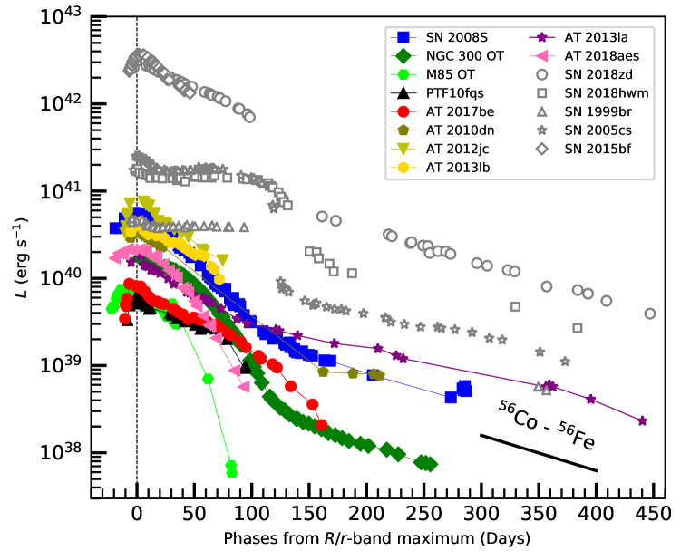
Figure 5: Pseudo-bolometric $B$ to $I/i$ light curves of ILRTs and comparison objects. The dashed vertical line indicates the time of $R/r$-band maximum light.

The bolometric light curve is computed by integrating the spectral energy distribution (SED) over the whole electromagnetic spectrum. However, in most cases, observations at wavelengths shorter than the $u$ band, and longer than $I/i$-band are not available. For this reason, to achieve meaningful comparisons among ILRTs, we computed pseudo-bolometric light curves including only the contribution from the $B$ to the $I/i$ band. We first converted the extinction-corrected magnitudes to flux densities, and finally integrated the SEDs at their effective wavelengths, assuming a negligible flux contribution outside of the integration region. The resulting pseudo-bolometric light curves are presented in Figure 5, while peak luminosities are reported in Table 3. They show faint peak luminosities ranging from $0.5\times 10^{40}$ erg s^-1 to $9.0\times 10^{40}$ erg s^-1. For comparison, the claimed EC SNe SN 2018zd and SN 2015bf have peak luminosities of $\sim$ $3.7\times 10^{42}$ erg s^-1 and the faint Type IIP SN 1999br is about $4.7\times 10^{40}$ erg s^-1 (see Figure 5). The pseudo-bolometric light curve shapes of ILRTs are broadly similar to Type IIP (in particular, PTF10fqs and AT 2017be) and/or Type IIL (SN 2008S and AT 2012jc) SNe, as demonstrated in Figure 5. In analogy to Type IIP SNe, the light curves for ILRTs are influenced by a number of factors, such as the presence of a CSM, the H recombination timescale, and ⁵⁶Ni distribution. Finally, we perform a non-parametric fit using the ReFANN code (Wang et al., 2020, 2021) to reconstruct the pseudo-bolometric light curve, and integrate it over the covered photometric evolution. The resulting radiated energies are in the range of (0.30 - 2.94) $\times$ 10⁴⁷ erg, with values reported in Table 3. These values should be regarded as lower limits due to our incomplete wavelength coverage and limited temporal coverage. These observed ILRTs radiated energies are fractions of about 10^-4 - 10^-3 of the theoretical predictions for the explosion energy of EC SNe (about 10⁵⁰ erg, Kitaura et al., 2006; Wanajo et al., 2009; Tominaga et al., 2013). Stritzinger et al. (2020b) pointed out that theoretical EC SN simulations may overpredict the explosion energy. Therefore, this discrepancy should be considered in future observations and modelling efforts.

In order to provide reliable estimates for the ejected ⁵⁶Ni masses, we need to compute the bolometric light curves. Unfortunately, most objects do not have MIR observations, and optical and/or NIR light-curve information is sometimes incomplete at late times. SN 2008S and NGC 300 OT are exceptions, as they were followed until late phases, and also have MIR coverage. Observations of these two objects revealed that the SEDs of ILRTs shift from the optical to the MIR domain, with the MIR being dominant at late phases (e.g. Botticella et al., 2009; Kochanek, 2011). To mitigate the limited observational information available for other objects, we adopted SN 2008S as a template for other ILRTs, and assumed that all others share the same SED evolution. Hence, we used SN 2008S to determine the bolometric corrections for all ILRTs that had incomplete wavelength coverage. We estimated the optical and NIR luminosity contribution of SN 2008S, using the bolometric light curve model ($L_{\rm{bol}}=L_{0}\times\exp(-t/t_{0})$ + $L_{1}$, with $L_{0}\simeq 10^{7.3}L_{\odot}$, $L_{1}\simeq 10^{5.8}L_{\odot}$ and $t_{0}\simeq 48$ days) from Kochanek (2011). We first computed the $\frac{L_{\rm{opt}}}{L_{\rm{bol}}}$, $\frac{L_{\rm{NIR}}}{L_{\rm{bol}}}$, and $\frac{L_{\rm{opt}}+L_{\rm{NIR}}}{L_{\rm{bol}}}$ ratios at late phases for SN 2008S. The $L_{\rm{opt}}$, $L_{\rm{NIR}}$, and $L_{\rm{opt}}+L_{\rm{NIR}}$ contributions for other ILRTs at the same phases were then calculated, assuming the same ratios as for SN 2008S. Specifically, $L_{\rm{bol}}$ was computed starting from the measured $L_{\rm{opt}}+L_{\rm{NIR}}$ for AT 2010dn, from $L_{\rm{opt}}$ for AT 2013la, and $L_{\rm{NIR}}$ for AT 2017be, and then by applying the adopted bolometric corrections.

Assuming that the late-time evolution of ILRTs are powered by the radioactive decay chain ⁵⁶Ni $\to$ ⁵⁶Co $\to$ ⁵⁶Fe, the late-time luminosity of ILRTs can be used to constrain the synthesised ⁵⁶Ni mass. We use the well-observed Type II SN 1987A as a reference (Catchpole et al., 1988; Whitelock et al., 1988; Catchpole et al., 1989) and estimate the ejected ⁵⁶Ni mass of ILRTs using Equation 2:

$$M\left({}^{56}\mathrm{Ni}\right)_{\mathrm{ILRT}}\leavevmode\nobreak\ $=$M\left({}^{56}\mathrm{Ni}\right)_{\mathrm{SN\leavevmode\nobreak\ 1987A}}\times\left(L_{\mathrm{ILRT}}\left(t\right)\over L_{\mathrm{SN\leavevmode\nobreak\ 1987A}}\left(t\right)\right),$$ (2)

where $M(^{56}\mathrm{Ni})_{\mathrm{SN\leavevmode\nobreak\ 1987A}}\sim 0.073\leavevmode\nobreak\ \mathrm{M_{\odot}}$ is the ⁵⁶Ni mass synthesised by SN 1987A, and $L_{\mathrm{ILRT}}$ and $L_{\mathrm{SN\leavevmode\nobreak\ 1987A}}$ are late-time luminosities of an individual ILRT and SN 1987A, respectively. Hereafter, we only consider five ILRTs that have observations in the nebular phase. Because of the poor constraints on the explosion epoch of ILRTs, we use the last non-detection and the first detection to fix the earliest and the latest possible extremes for the explosion epochs. Hence, we obtain upper and lower limits of ⁵⁶Ni masses for the ILRTs, reported in Table 3. SN 2008S ejected the largest amount of ⁵⁶Ni ($3.2$ - $3.5\times 10^{-3}$ M_⊙ ), while AT 2017be has the lowest ⁵⁶Ni mass ($6.7$ - $7.2\times 10^{-4}$ M_⊙ ). All inferred ⁵⁶Ni masses are of the order of $10^{-4}$ to $10^{-3}$ M_⊙ , which, as discussed in Sect. 6, is in agreement with the predictions for EC SNe.

3.5 Evolution of the SED of ILRTs: the test case of AT 2010dn

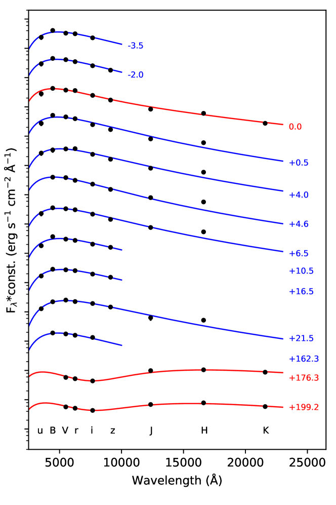
Figure 17: SED evolution of AT 2010dn. The lines are the best-fit BBs, which are overplotted on each SED. Blue lines are the fits of the single BB, while red lines are the fits of the double BB. The epochs marked to the right of each SED are relative to the $r$-band maximum. Each SED has been sifted by an arbitrary constant for clarity.

It is well known that SN 2008S, NGC 300 OT, and AT 2012jc already showed an IR excess soon after their discovery (Botticella et al., 2009; Humphreys et al., 2011; Stritzinger et al., 2020b). If we assume their progenitors to be embedded in complex and extended dusty environments, we should expect such IR excesses to be frequently observed for ILRTs. This can be verified in the case of AT 2010dn, for which MIR observations are available. Using the light curves presented in Table 8, 9, and 10, we constructed the SEDs of AT 2010dn at different epochs using photometry from the optical to the MIR. The first optical to MIR SED is obtained at $t\sim$30.6 days after maximum, which clearly reveals an IR excess over a single black body (BB) model (see the top panel of Figure 6). Hence, the SED was fitted with two-component (hot+warm components) BB functions instead of a single one. The hot component has a temperature $T_{\mathrm{hot}}$=5390 $\pm$ 70 K and a radius $R_{\mathrm{hot}}\approx 2.87\times 10^{14}$ cm, while the warm component has $T_{\mathrm{warm}}$ $\approx$ 970 K and $R_{\mathrm{warm}}\approx 4.63\times 10^{15}$ cm. In comparison, SN 2008S had $T_{\mathrm{hot}}$= 8076 $\pm$ 150 K, $R_{\mathrm{hot}}=(2.1\pm 0.1)\times 10^{14}$ cm, $T_{\mathrm{warm}}$ $\approx$ 585 K, $R_{\mathrm{warm}}\approx 9.9\times 10^{15}$ cm at maximum (Botticella et al., 2009), while AT 2012jc had a BB temperature of $T_{\mathrm{hot}}$ $\approx$ 6430 K and $T_{\mathrm{warm}}$ $\approx$ 800 K at + 26.8 days (Stritzinger et al., 2020b). The hot-component estimates are consistent with emission from the photosphere, while the warm component peaking in the MIR domain is likely due to circumstellar dust. For AT 2010dn, additional epochs of SEDs along with the corresponding best-fit BB functions are shown in Figure 17 (Appendix C), while the first BB parameters are reported in Table 11. The $T_{\mathrm{hot}}$ increases to $\sim$ 6490 K and, when the luminosity fades, $T_{\mathrm{hot}}$ also declines to $\sim$ 3540 K at $+$199.2 d. The $R_{\mathrm{hot}}$ shows a slow evolution (from 2.4 to 2.9 $\times 10^{14}$ cm) until $+$21.5 d, and declines to 1.6 $\times 10^{14}$ cm at $+$199.2 d. Three epochs with K band data reveal a possible second warm component with an almost constant temperature of 1100-1200 K (see Figure 17).

We also measured the residual flux at the location of AT 2010dn in Spitzer MIR images taken more than 3 years (+1333 days) after the outburst, and constructed a very late-time SED. This SED can be reproduced by a single BB function with a characteristic temperature of 440 K (see the bottom panel of Figure 6). We caution that this temperature should be regarded as an indicative value because of the limited coverage of MIR data. Similarly, AT 2012jc has very late-phase (+1155 days) Spitzer MIR photometric fluxes suggesting a BB temperature of about $600\,\rm{K}$. Based on the similarity of these three cases, we suggest that this SED evolution seems to be typical of ILRTs. A plausible explanation is that a dusty environment has formed through mass-loss events prior to the ILRT outbursts, in analogy to what is frequently observed in a few CC SNe (e.g. SN 1995N, SN 1998S, SN 2010jl, SN 2014ab, SN 2015da; see Gerardy et al., 2002; Andrews et al., 2011; Fransson et al., 2014; Tartaglia et al., 2020; Moriya et al., 2020). The slowly declining IR flux lasting around 4 years suggests that the outer dust shell was not destroyed by the radiation field emitted by the luminous outburst (regardless of the physical mechanism that produced the ILRTs; Botticella et al., 2009).

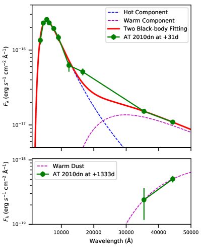
Figure 6: Top panel: Two-component black body fits to the SED of AT 2010dn obtained from optical to MIR at the epoch of +30.6 days. Bottom panel: Single black body fit for AT 2010dn in the MIR domain at very late phase of +1332.5 days. Although this fit could reproduce the late MIR data, the fitted temperature should be considered as an indicative value. The MIR measurements were obtained from the Spitzer Space Telescope + IRAC images at 3.6 $\mu$m and 4.5 $\mu$m.

Table 4: Log of spectroscopic observations of ILRTs.

Date	MJD	Phasea	Telescope+Instrument	Grism	Spectral range	Resolution	Exp. time
		(d)			($\AA$)	($\AA$)	(s)
AT 2010dn
20100602	55349.9	-5.0	TNG+LRS	LR-R	5090 - 8340	10.5	2100
20100603	55350.9	-4.0	TNG+LRS	LR-B	3300 - 7990	13.5	3000
20100604	55351.9	-3.0	TNG+LRS	VHR-R	6170 - 7780	3.2	2700
20100605	55352.9	-2.0	TNG+LRS	VHR-I	7290 - 8870	3.5	2700
20100607	55354.9	+0.0	WHT+ISIS	R300B/R158R	3160 - 10300	4.1/6.8	1800/1800
20100609	55356.9	+2.0	NOT+ALFOSC	gm4	3630 - 8960	18	3600
20100611	55358.9	+4.0	TNG+LRS	LR-B	3520 - 7990	11	2700
20100616	55363.9	+9.0	TNG+LRS	VHR-R	6190 - 7820	3.2	3000
20100617	55364.9	+10.0	TNG+LRS	VHR-R	6190 - 7820	3.2	3000
20100707	55384.9	+30.0	WHT+ISIS	R300B/R316R	3160 - 8860	4.1/3.1	1200/1200
AT 2012jc
20120329	56015.1	$-8.4$	Ekar1.82 + AFOSC	gm4	3500 - 8060	24	3600
20120331	56017.3	$-6.2$	Ir$\rm{\acute{e}}$n$\rm{\acute{e}}$e du Pont + WFCCD	blue (400/mm)	3600 - 9120	5.3	1500
20120414	56031.2	$+7.7$	NTT + EFOSC2	Gr$\#$11/Gr$\#$16	3340 - 9920	21.3/21	1800
20120501	56048.3	$+24.8$	NTT + EFOSC2	Gr$\#$11/Gr$\#$16	3340 - 9920	14/13	1800
20120623	56101.2	$+77.7$	Magellan II + LDSS	VPH-All	3940 - 10300	6.5	900
AT 2013lb
20130207	56330.1	$+5.6$	Ekar1.82 + AFOSC	gm4	3900 - 8200	14	2700
20130207	56330.4	$+5.9$	NTT + EFOSC2	Gr$\#$13	3650 - 9090	17	1213
20130207	56330.4	$+5.9$	Gemini-S + GMOS-S	R400	4210 - 8440	10	900
20130209	56332.3	$+7.8$	NTT + EFOSC2	Gr$\#$11	3340 - 7460	22	1394
20130220	56343.3	$+18.8$	NTT + EFOSC2	Gr$\#$11	3340 - 7460	22	2700
20130305	56356.3	$+31.8$	NTT + EFOSC2	Gr$\#$11/Gr$\#$16	3340 - 9990	14/13	2700
20130422	56404.3	$+79.8$	Gemini-S + GMOS-S	R400	4210 - 8440	10	450
AT 2013la
20140108	56665.2	$+13.2$	Ekar1.82 + AFOSC	gm4	3400 - 8200	14	1800
20140115	56672.2	$+20.2$	Pennar1.22 + B&C	300tr	3350 - 7930	10	1800
20140203	56692.2	$+40.2$	TNG+LRS	LR-B	3430 - 8050	10.5	3600
20140205	56694.2	$+42.2$	GTC + OSIRIS	R500R	5150 - 9990	15.5	2700
20140228	56717.2	$+65.2$	GTC + OSIRIS	R1000B	3650 - 7850	7	900
20140322	56739.1	$+87.1$	TNG+LRS	LR-B	3430 - 8050	10.5	2700
20140716	56854.9	$+202.9$	GTC + OSIRIS	R1000B	3650 - 7850	7	1500
20140814	56883.9	$+231.9$	GTC + OSIRIS	R1000B	3650 - 7850	7	1900
20141220	57012.3	$+360.3$	GTC + OSIRIS	R1000B	3650 - 7850	7	1800
AT 2018aes
20180331	58208.1	$-3.0$	GTC + OSIRIS	R1000B/R	3630 - 10080	7.5	600/600
20180426	58234.1	$+23.0$	GTC + OSIRIS	R1000B/R	3630 -10340	7.5	600/600

^a Phases are relative to the $R/r$-band peak.

4 Spectroscopy

Our spectral sequences for AT 2010dn, AT 2012jc, AT 2013lb, AT 2013la and AT 2018aes were obtained using multiple instrumental configurations, which are listed in Appendix A (Table 6). Basic parameters for the spectra are reported in Table 4.

The spectra were processed with the standard procedures in iraf. The preliminary reduction steps included bias, overscan and flat-field corrections. We then extracted 1D spectra from the 2D frames using the task apall. Wavelength calibration of the 1D spectra was performed with arc lamp spectra obtained with the same instrumental configuration as the science ones. The spectra of spectro-photometric standard stars were used to estimate a sensitivity function curve necessary to flux-calibrate the spectra of the transients. The accuracy of the flux calibration was then checked against coeval broadband photometry, and correction factors were applied in case of discrepancy. The spectra of the standard stars were also used to correct for the telluric absorption bands (e.g. O₂ and H₂O) from the ILRTs spectra. The resulting ILRT spectra are shown in Figure 7.

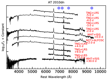
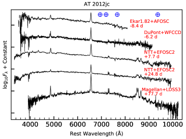
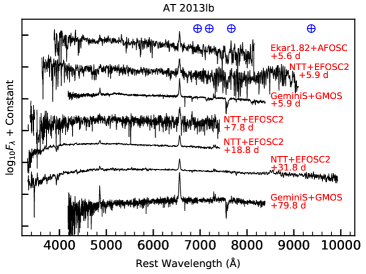
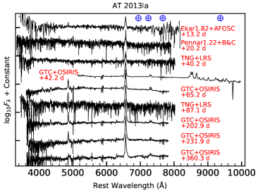
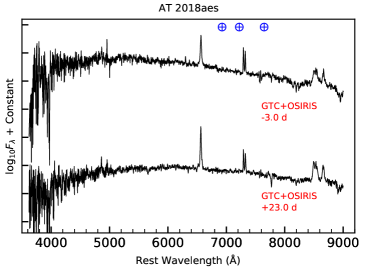
Figure 7: Spectral evolution of AT 2010dn (top-left), AT 2012jc (top-right), AT 2013lb (middle-left), AT 2013la (middle-right), and AT 2018aes (bottom). The epochs marked to the right of each spectrum are relative to the $R/r$-band maximum. The $\bigoplus$ symbols mark the position of the strongest telluric absorption bands. The spectra are only corrected for redshift.

Table 5: Physical parameters inferred from the optical spectra of the ILRTs sample.

Date	MJD	Phasea	$v$ (H$\alpha$) b	$L$ (H$\alpha$) c	$L_{\rm{H_{\alpha}}}$/$L_{\rm{[{\mathrm{Ca\,\mathsc{\leavevmode\nobreak\ }}}II]}}$ c	$T_{\mathrm{BB}}$
		(d)	(km s-1)	(1038erg s-1)		(K)
AT 2010dn
20100602	55349.9	$-5.0$	695	2.12	2.9	7095 $\pm$ 355
20100603	55350.9	$-4.0$	671	1.85	2.6	6890 $\pm$ 240
20100604	55351.9	$-3.0$	588	3.47	2.5	6540 $\pm$ 330
20100605	55352.9	$-2.0$	–	–	–	6435 $\pm$ 320
20100607	55354.9	$+0.0$	577	2.29	2.6	6760 $\pm$ 340
20100609	55356.9	$+2.0$	$<$823	2.63	2.5	6830 $\pm$ 340
20100611	55358.9	$+4.0$	563	1.86	2.3	6690 $\pm$ 195
20100616	55363.9	$+9.0$	442	2.12	2.2	6820 $\pm$ 320
20100617	55364.9	$+10.0$	438	1.81	2.1	6710 $\pm$ 280
20100707	55384.9	$+30.0$	$<$142	0.58	1.8	5020 $\pm$ 250
AT 2012jc
20120329	56015.1	$-8.4$	$<$1097	5.30	–	8380 $\pm$ 420
20120331	56017.3	$-6.2$	614	5.30	15.4	7385 $\pm$ 740
20120414	56031.2	$+7.7$	$<$960	5.27	10.2	7995 $\pm$ 205
20120501	56048.3	$+24.8$	$<$617	2.97	5.5	6780 $\pm$ 340
20120623	56101.2	$+77.7$	842	2.36	–	5445 $\pm$ 525
AT 2013lb
20130207	56330.1	$+5.6$	$<$640	3.33	–	6865 $\pm$ 685
20130207	56330.4	$+5.9$	$<$777	3.36	13.4	6450 $\pm$ 645
20130207	56330.4	$+5.9$	$<$460	3.29	–	6250 $\pm$ 315
20130209	56332.3	$+7.8$	$<$1006	–	–	5850 $\pm$ 585
20130219	56343.3	$+18.8$	$<$1006	2.29	8.2	6390 $\pm$ 640
20130304	56356.3	$+31.8$	$<$617	1.87	4.8	6450 $\pm$ 325
20130422	56404.3	$+79.8$	680	2.33	–	4375 $\pm$ 220
AT 2013la d
20140108	56665.2	$+13.2$	$<$640	6.31	–	5880 $\pm$ 295
20140115	56672.2	$+20.2$	$<$457	5.92	–	7110 $\pm$ 1420
20140203	56692.2	$+40.2$	778	–	–	6050 $\pm$ 1210
20140205	56694.2	$+42.2$	$<$709	5.33	–	5345 $\pm$ 270
20140228	56717.2	$+65.2$	400	4.99	–	5290 $\pm$ 265
20140322	56739.1	$+87.1$	$<$480	5.04	–	6005 $\pm$ 1200
20140716	56854.9	$+202.9$	446	3.98	–	5055 $\pm$ 255
20140814	56883.9	$+231.9$	503	3.87	–	4285 $\pm$ 225
20141220	57012.3	$+360.3$	499	2.68	–	4485 $\pm$ 180
AT 2018aes
20180331	58208.1	$-3.0$	708	0.85	2.7	6620 $\pm$ 330
20180426	58234.1	$+23.0$	609	0.77	2.2	5675 $\pm$ 285

^a Phases are relative to the $R/r$-band light curve peaks.
$b$ Most of our measurements are limited by the instrumental resolution constraints, hence the FWHM velocities may have large error bars, and in many cases they should be regarded as upper limits.
$c$ We adopt conservative errors of $\sim$20% for the H$\alpha$ luminosity and the $L_{\rm{H_{\alpha}}}$/$L_{\rm{[{\mathrm{Ca\,\mathsc{\leavevmode\nobreak\ }}}II]}}$ ratio because of the uncertainty in the flux calibration of the spectra.
$d$ H$\alpha$ has a complex profile in AT 2013la, and was therefore fitted with multiple components. The narrowest Gaussian emission and absorption components are usually below the instrumental resolution limit. For this reason, only the FWHM velocities of the broader Lorentzian components are reported here.

4.1 Spectroscopic evolution and line identification

The five objects of our sample have spectra showing little evolution over the period of their spectral monitoring (from $\sim-8$ days to 1 year after maximum). At all epochs, the spectra have an almost featureless continuum, which is relatively blue at early phases, becoming redder with time. Narrow emission lines of the Balmer series are superposed on the continuum, with H$\alpha$ and H$\beta$ being the most prominent spectral features. Weak Fe ii lines are also observed, along with Na I D and Ca H&K in absorption. Apart from the H lines, the most prominent spectral emissions are the [Ca ii] doublet ($\lambda\lambda$ 7291, 7324) and the Ca NIR triplet ($\lambda\lambda$ 8498, 8542, 8662). In addition, O i, Fe ii, Sc ii and Ba ii lines are also tentatively identified in some spectra with decent S/N and resolution (e.g. see a GTC/OSIRIS spectrum at + 41.9 d of AT 2013la). Detailed line identification performed on the best-quality spectra of the five transients is given in Figure 8. We note that the lines of the [Ca ii] doublet are visible in all spectra with good S/N shown in this paper and are therefore considered a characteristic feature of ILRTs. In Figure 9, all ILRTs share almost the same spectral features, supporting a remarkable overall homogeneity in their observables. However, as shown in Figure 9, the spectra of the comparison objects show much bluer continuum than ILRTs. In addition, H$\alpha$ has a classical broad P-Cygni profile and there is no obvious [Ca ii] doublet feature.

During the follow-up campaign of AT 2013la, we collected spectra covering all the evolutionary phases. Hence, we take AT 2013la as a representative object to describe the spectral evolution of ILRTs. The spectral continuum evolves quite slowly, from initially blue (e.g. at phase $\sim$ +13.2 d) to much redder at late phases (+360.0 d). AT 2013la resembles other ILRT spectra in its continuum evolution and characteristic lines. However, we see additional strong He I (5876 $\AA$) absorption feature in all GTC/OSIRIS spectra, most clearly at +42.2, +65.2, +202.9, +231.9, and +360.3 days (see middle right panel in Figure 7). We note that narrow P-Cygni absorptions imposed on H$\alpha$ lines are also detected in the highest resolution spectra (see e.g. the GTC/OSIRIS spectra of AT 2013la in Figures 7 and 25). Such spectra allow us to infer the wind velocity via measurement of the position of the deep minimum of the P-Cygni profiles. This blueshifted absorption component on top of the H$\alpha$ emission (see Figure 25) has velocities of $\sim$ 360 - 410 $\rm{km}\,s^{-1}$, and may originate from a dense, slow-moving wind. This is discussed more widely in Sect. 4.2.

We assume that the SEDs of ILRTs in the optical domain covered by our spectra are approximated by black bodies. Therefore, we estimate the temperature through a black body fit to the spectral continuum. The inferred continuum temperatures are reported in Table 5, while the temperature evolution is shown in the top panel of Figure 10. For all objects in our sample, the temperature rapidly declines from $\sim$ 7000 - 8500 K near maximum, to nearly 5000 K at $\sim$ 100 days. At late phases, the temperature decreases more slowly to $\sim$ 4200 - 4500 K at about 1 year after maximum. Overall, all our ILRTs show a similar temperature evolution. We note that the comparison objects show much higher temperatures than ILRTs at early phases, and this is consistent with their early-time bluer colours.

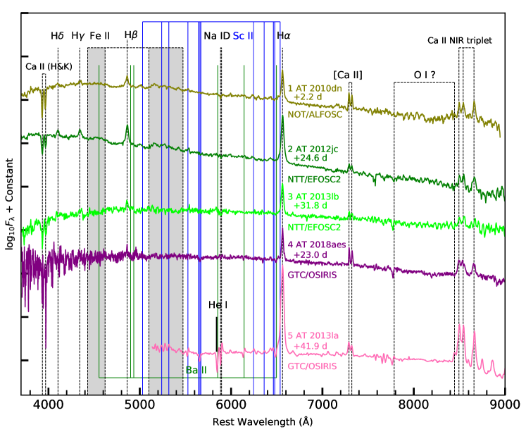
Figure 8: Line identification in the spectra of the five transients presented in this paper. The spectra have been corrected for redshift and reddening. Phases are relative to their $R/r$-band maximum.

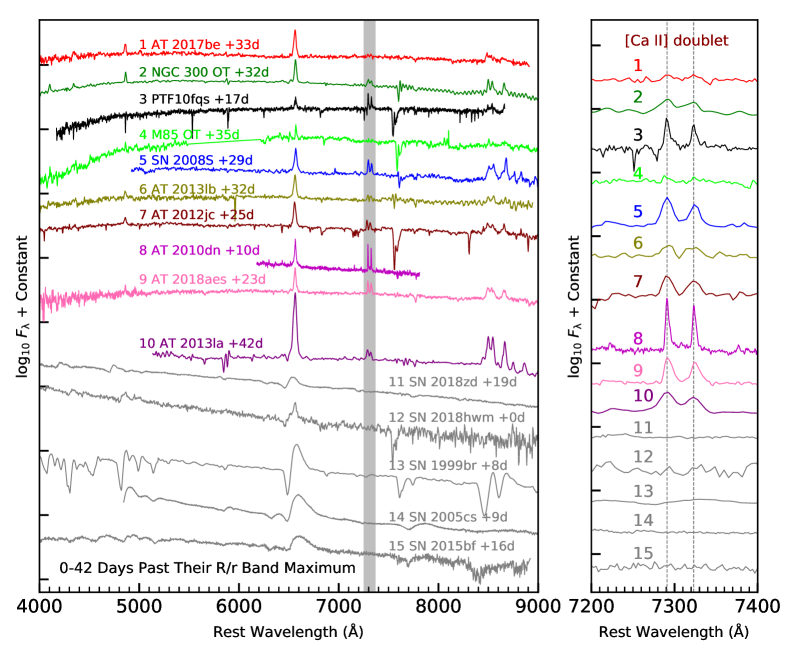
Figure 9: Spectral comparison of a sample of ILRTs and SN 2018zd, SN 2018hwm, SN 2015bf, SN 1999br, and SN 2005cs. The spectra of M85 OT, SN 2008S, PTF10fqs, AT 2017be, SN 2018zd, SN 2018hwm, SN 2015bf, SN 1999br, and SN 2005cs are taken from Kulkarni et al. (2007), Botticella et al. (2009), Kasliwal et al. (2011), Cai et al. (2018), Zhang et al. (2020), Reguitti et al. (2021), Lin et al. (2021), Pastorello et al. (2004), and Pastorello et al. (2006, 2009). The right panel shows the region of [Ca ii], marked with the grey-shaded region in the left panel. All spectra were obtained at similar epochs from the $R/r$-band maxima, and were corrected for redshift and reddening.

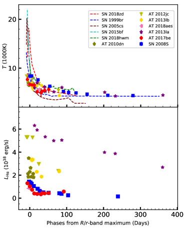
Figure 10: Evolution of the black body temperature (top) and the H$\alpha$ luminosity (bottom) for a sample of ILRTs, and SN 2018zd (Zhang et al., 2020), SN 2018hwm (Reguitti et al., 2021), SN 2015bf (Lin et al., 2021), SN 1999br (Pastorello et al., 2004), and SN 2005cs (Pastorello et al., 2006, 2009).

4.2 H$\alpha$ and Ca ii line evolution

In order to understand the evolution of individual spectral features, we performed a detailed analysis of the spectra of our ILRT sample at three critical phases: around 0, +30, and +70 days from maximum (see Figure 25). We measure the full width at half maximum (FWHM) of H$\alpha$ through a single Lorentzian function fit, as in general this type of fit accurately describes the line profiles of narrow-lined SNe (e.g. SNe IIn; see Taddia et al., 2013; Smith, 2017; Nyholm et al., 2017). The H$\alpha$ profile is dominated by a narrow component in the spectra of most objects (e.g. AT 2010dn, AT 2012jc, AT 2013lb, and AT 2018aes). However, AT 2013la shows H$\alpha$ with a more complex profile, with narrow, blueshifted P-Cygni absorption lines. For AT 2013la, we therefore fitted the H$\alpha$ emission lines in our higher resolution spectra (i.e. at phases +65.2d, +202.9, +231.9 and +360.3d) via multiple components: an intermediate-width Lorentzian profile, a narrow Gaussian emission and a Gaussian absorption. We also fitted the H$\alpha$ line at phase +42.2d with only a broader Lorentzian component plus a narrow Gaussian. The narrow component of H$\alpha$ arises from the unshocked photoionised CSM, while the intermediate-width component likely originates from the shocked CSM. Finally, the broad component is produced by the faster ejecta. The FWHM velocities ($v_{\mathrm{FWHM}}$) of H$\alpha$, after correcting for instrumental resolution ($v_{\mathrm{FWHM}}$ = $\sqrt{v_{\mathrm{observation}}^{2}-v_{\mathrm{instrument}}^{2}}$), are reported in Table 5 and plotted in Figure 11. We note that most spectra of our sample have modest resolution. Hence, in most instances our measurements have to be considered upper limits for the expansion velocities. We also measured the H$\alpha$ velocity for the comparison objects in Figure 11, which were inferred from the minima of the broad P-Cygni absorptions. These show a remarkably large velocity evolution, ranging from $\sim$ 8000 $\rm{km}\,s^{-1}$ to $\sim$ 1000 $\rm{km}\,s^{-1}$. In contrast, ILRTs show a slow evolution in H$\alpha$ velocity ($<$ 1000 $\rm{km}\,s^{-1}$) over the entire monitoring campaigns. In Figure 12, we show the temporal evolution of H$\alpha$ profiles in the velocity space for AT 2013la, SN 2018zd, and SN 2005cs. AT 2013la shows a modest velocity evolution in H$\alpha$ profile, while SN 2018zd and SN 2005cs experience significant velocity evolution along with the gradual emergence of broad P-Cygni features.

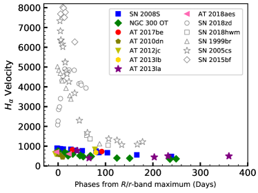
Figure 11: H$\alpha$ velocity evolution of a sample of ILRTs, SN 2018zd (Zhang et al., 2020), SN 2018hwm (Reguitti et al., 2021), SN 2015bf (Lin et al., 2021), SN 1999br (Pastorello et al., 2004), and SN 2005cs (Pastorello et al., 2006, 2009). The H$\alpha$ velocities were estimated by measuring the FWHM for ILRTs, while those for SNe II were determined from the position of the minimum of the absorption component.

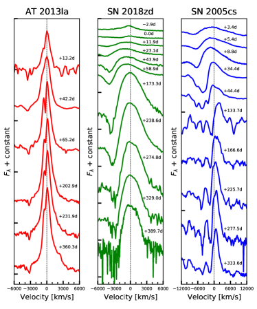
Figure 12: Evolution of the H$\alpha$ profile in selected spectra of the ILRT AT 2013la (left panel), SN 2018zd (Zhang et al., 2020, middle panel), and the underluminous Type IIP SN 2005cs (Pastorello et al., 2006, 2009, right panel). The H$\alpha$ lines are shown in the velocity space, with zero velocity (rest wavelength) being marked by a grey dashed line.

The [Ca ii] doublet and Ca ii NIR triplet lines were fitted with Lorentzian functions. The [Ca ii] doublet is produced by quadrupole transitions from $4s^{2}S$ to the metastable $3d^{2}D$ level, in which $\lambda_{1}$ at 7291 $\AA$ and $\lambda_{2}$ at 7324 $\AA$ are associated to ${}^{2}S_{1/2}$ - ${}^{2}D_{5/2}$ and ${}^{2}S_{1/2}$ - ${}^{2}D_{3/2}$ transitions, respectively (e.g. Osterbrock, 1951; Lambert et al., 1969; Chevalier & Fransson, 1994). The [Ca ii] doublet likely originates from extremely low-density gas, possibly in a slow-moving circumstellar shell. The Ca ii NIR triplet lines with $\lambda$_1,2,3= 8498, 8542, 8662 Å are common features in many cool transients, and are produced by transitions from $4p^{2}P_{1/2,3/2}$ to $3d^{2}D_{3/2,5/2}$ levels (e.g. Mallik, 1997, 1998; Andretta et al., 2005; Busà et al., 2007; Martin et al., 2017).

At early phases (see Figure 25, left panel), the H$\alpha$ FWHM velocities of the transients presented in this paper are 600-700 $\rm{km}\,s^{-1}$ (with upper limits up to 1000 $\rm{km}\,s^{-1}$ in cases of unresolved features), which are comparable to those of other ILRTs (e.g. $\sim$750 $\rm{km}\,s^{-1}$ and $\sim$600 $\rm{km}\,s^{-1}$ for SN 2008S and AT 2017be, respectively). We conclude that in all ILRTs the ejected material expands with similar velocities of several hundred $\rm{km}\,s^{-1}$. In most cases the FWHM of the [Ca ii] doublet is below the resolution limits, and we do not have reliable estimates for the outflow velocity inferred from this feature. The doublet is resolved only in the spectra of AT 2010dn at $-3.0$ d, providing an FWHM velocity of 145 $\rm{km}\,s^{-1}$. The feature was also resolved in a spectrum of AT 2012jc at phase $-$6.2 d, where we measured $v_{\mathrm{FWHM}}$ $\sim$ 220 $\rm{km}\,s^{-1}$. For AT 2018aes, a velocity of $v_{\mathrm{FWHM}}$ $\sim$ 310 $\rm{km}\,s^{-1}$  was derived for the [Ca ii] feature at phase -3.0 d. We conclude that the [Ca ii] doublet originates in a slow-moving CSM ($\sim$ 145 - 310 $\rm{km}\,s^{-1}$), while the broader H$\alpha$ component forms in fast-expanding ejected gas.

At 3-5 weeks after maximum (Figure 25, middle panel), the spectra become redder. We also see a strengthening of a narrow P-Cygni profile superimposed on H$\alpha$ in AT 2013la, the minimum of which is blueshifted by about 360 - 410 $\rm{km}\,s^{-1}$. However, we cannot rule out that the non-detection of this feature in other objects is a mere resolution effect. The FWHM velocities of H$\alpha$ are in the range 600-850 $\rm{km}\,s^{-1}$ for all objects, with M85 OT being the only outlier with $v_{\mathrm{FWHM}}$ $\sim$ 350 $\rm{km}\,s^{-1}$. A resolved velocity of 115 $\rm{km}\,s^{-1}$ was reported at this phase for [Ca ii] in AT 2017be (Cai et al., 2018).

At late phases (+70 to +80 d; Figure 25, right panel), the H$\alpha$ velocity does not change significantly, still ranging from 400 (in AT 2013la) up to 850 $\rm{km}\,s^{-1}$ (in the other objects). The spectra of AT 2013la also provide an averaged [Ca ii] $v_{\mathrm{FWHM}}$ $\sim$ 365 $\rm{km}\,s^{-1}$. In most cases, the low resolution or the low S/N of our spectra prevent us from probing the Ca ii triplet lines in detail, with an exception being the Magellan spectrum of AT 2012jc obtained on 2012 June 23 (phase +77.7 d), where the triplet emission lines show a symmetric profile, with an average $v_{\mathrm{FWHM}}$ $\simeq$ 905 $\rm{km}\,s^{-1}$. The [Ca ii] profile appears to show very little evolution in the FWHM until $t\sim$ 70 days, and this is a further argument in favour of the hypothesis that these lines form in the circumstellar environment. We also note that none of the typical nebular lines, such as [O iii] ($\lambda\lambda$= 4959, 5007 Å) and [S ii] ($\lambda\lambda$= 6716, 6731 Å) lines (Lundqvist & Fransson, 1996; Lundqvist et al., 2015, 2020), were detected in spectra. This implies that the wind density is high enough for those nebular lines to be collisionally de-excited, but that [Ca ii] can exist at much higher density (e.g. critical density: $\rho$${}_{\rm{[S\leavevmode\nobreak\ II]}}$ = 1 $\times$ 10⁴ cm^-3, $\rho_{\rm{[Ca\leavevmode\nobreak\ II]}}$ = 1 $\times$ 10⁹ cm^-3; Li & McCray, 1993). In such a dense wind, the [Ca ii] lines could also be broadened by Thomson scattering, albeit to a lesser extent than the Balmer lines because these latter are formed further out in the wind/CSM.

We use the few spectra with higher S/N to highlight the evolution of the H$\alpha$ to [Ca ii] luminosity ratio. The values for the different ILRTs are reported in Table 5 and shown in Figure 14. The values for AT 2012jc and AT 2013lb show a faster decline (by a factor of three) from maximum (when H$\alpha$ largely dominates) to one month later. However, for AT 2010dn and AT 2018aes, the above ratio shows a much flatter evolution (ratio from about 3 to 2) over the same temporal window. Interestingly, in these two ILRTs, the [Ca ii] doublet is very luminous with respect to H$\alpha$. In addition, the H$\alpha$ luminosity evolution is also shown in the bottom panel of Figure 10.

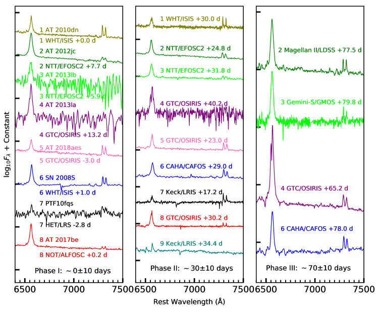
Figure 13: Evolution of H$\alpha$ and [Ca ii] in ILRTs. The spectra of M85 OT, SN 2008S, PTF10fqs, and AT 2017be, downloaded from WISeREP archive  (Yaron & Gal-Yam, 2012), were published by Kulkarni et al. (2007), Botticella et al. (2009), Kasliwal et al. (2011), and Cai et al. (2018). All spectra were corrected for redshift and reddening.

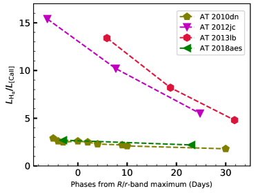
Figure 14: Ratio of H$\alpha$ to [Ca ii] (total profiles at $\lambda\leavevmode\nobreak\ \approx$ 7300 Å) luminosities until phase $\sim$ 30 d.

5 Rate estimates for ILRTs

In the past 12 years (2008 - 2019), 12 objects have been confirmed to be ILRT events; the observed rate of discoveries is 1.0 event per year, but this does not account for the luminosity distribution of ILRTs, or the efficiency or observing strategy of the surveys. The ILRTs in our sample are distributed in a radius of 30 Mpc, corresponding to a volume of 1.13 $\times$ 10⁵ Mpc³. Hence, we obtain a volumetric rate of ILRTs of 0.09 $\times$ 10^-4 Mpc^-3yr^-1. In the same temporal window and volume, 147 CC SNe were discovered corresponding to a rate of 1.1 $\times$ 10^-4 Mpc^-3yr^-1. Therefore, assuming that the discovery of ILRTs suffers the same selection effects as all CC SNe, the rate of ILRTs is 8% that of CC SNe. We note that Thompson et al. (2009) estimated an EC SN rate of 2%-10% of CC SNe in 10 years (before 2008), while Poelarends et al. (2008) obtained an EC SN fraction of CC SNe of only about 6% based on a standard Salpeter initial mass function (IMF; Salpeter, 1955) and an EC SN mass range of 9.00 - 9.25 M_⊙ . Assuming a narrow mass range $\Delta\approx$ 0.2 M_⊙  and a metallicity range $Z$ = 0.0001 - 0.02, Doherty et al. (2015, 2017) calculated that 2%-5% of CC SNe are EC SNe. However, theoretical estimates for EC SN rates are dependent on the uncertainties on the initial mass range, metallicity, and the details of stellar models. While theoretical calculations show some variations, they are roughly consistent with our rate estimate based on the observations. We note that we did not take into account the fact that ILRTs are on average fainter than CC SNe and surveys are incomplete up to 30 Mpc. Therefore, the true relative rate is larger than the current observed rate, and future advanced surveys could increase this estimate.

6 Discussion and conclusions

6.1 Observables and parameter correlations

In this paper, we systematically analyse a sample of ILRTs. They show relatively homogeneous spectrophotometric properties that can be summarised as follows:

1. They all show single-peaked light curves, resembling those of Type IIP/IIL SNe but scaled down in luminosity (see Figure 4). The duration of the plateau is determined by the effective recombination time of the hydrogen envelope (e.g. see Grassberg et al., 1971; Eastman et al., 1994; Soma et al., 2010).
   

2. They show a homogeneous colour (hence temperature) evolution. The temperature evolution shows an initial fast decline (usually lasting $<$30 days), followed by a much slower decline which is still ongoing at the end of the follow up. The temperature evolution of ILRTs is similar to what is observed in the hydrogen recombination of classical Type II SNe (e.g. see the Type IIP SN 2005cs in the top panel of Figure 10). We note that ILRTs are usually redder than low-luminosity SNe IIP and other Type II events proposed to be EC SN candidates (see Figure LABEL:pic:colour).
   

3. Their peak magnitudes range from $-$11 ($\pm$ 0.5) to $-$15 ($\pm$ 0.5) mag. Their quasi-bolometric ($B$ to $I$) light curve peaks are in the range $\sim 5\times 10^{39}$ to $\sim 9\times 10^{40}$ erg s^-1 and the radiated energies span from 0.30 $\times$ 10⁴⁷ to 2.94 $\times$ 10⁴⁷ erg. ILRTs are typically fainter than most SNe II, although they are comparable in luminosity to the most subluminous Type IIP SN 1999br (see Figure 4 and 5).
   

4. The SED of ILRTs with optical to MIR observations shows evidence of prominent IR excesses both at early and late phases. This is consistent with the expectation that the progenitors of ILRTs have dusty local environments. Furthermore, it corroborates the use of the nomenclature: ‘red’ transients. Another common feature in the SED evolution of ILRTs is the monotonic decrease of the photospheric radius, which could be a diagnostic tool to distinguish ILRTs from LRNe (see Figure 4 of Cai et al., 2019).
   

5. Their spectra experience relatively slow evolution. Prominent lines include the Balmer series, along with Ca ii (e.g. Ca H&K, [Ca ii] doublet, and Ca NIR triplet), Na i D, Fe ii, and possibly O i. The [Ca ii] doublet is normally visible during the entire monitoring campaign. However, the study of AT 2019abn challenges this paradigm with a barely detectable [Ca ii] doublet at early phases (Jencson et al., 2019; Williams et al., 2020). In addition, this feature is never detected in SNe IIP at early phases (see Figure 9), while it is always visible in the nebular phases.
   

6. The ejecta velocities inferred from the H$\alpha$ FWHM lie between about 400 and 800 $\rm{km}\,s^{-1}$. The measurements of the minimum of P-Cygni profiles indicate a modest wind velocity of about 360 - 410 $\rm{km}\,s^{-1}$. In addition, the [Ca ii] feature width suggests the existence of slow-moving CSM with $v_{\mathrm{FWHM}}$ $\sim$ 170 - 300 $\rm{km}\,s^{-1}$. In ILRTs, the H$\alpha$ velocity is much lower than those inferred for SNe II at all phases (see Figure 11).
   

In order to better characterise ILRTs, we looked for possible correlations among their physical parameters. In Figure 15, we plot peak luminosity ($L_{\rm{peak}}$; reported in Table 3) against different physical parameters of ILRTs, namely the time ($\Delta\mathrm{t}_{0.5}$) for the luminosity to decline by a factor of two from maximum, the ⁵⁶Ni mass, the H$\alpha$   velocity, and the H$\alpha$  luminosity at maximum. Unfortunately, several factors (e.g. poorly sampled light curve peaks; lack of late-time observations; low spectral resolution or modest S/N; incomplete wavelength coverage) limit the information available for the sample. More specifically, there seems to be no correlation between $L_{\rm{peak}}$ and decline time $\Delta\mathrm{t}_{0.5}$, which is in the range of 20-50 days (Figure 15, top-left panel). The lack of a correlation may point to variation in the progenitor mass loss or the strength of CSM-ejecta interaction. A trend may exist linking the peak luminosity to the ejected ⁵⁶Ni mass (Figure 15 top-right panel), although the lower limit for AT 2013la is somewhat discrepant with those of other ILRTs. We cannot rule out that the ejecta-CSM interaction significantly affects the late-time luminosity, therefore biasing the ⁵⁶Ni mass estimates of the sampled objects. The limited range of ⁵⁶Ni masses ($\sim$ 1-5 $\times 10^{-3}$ M_⊙ ) may be attributed to their progenitor masses lying within a narrow mass range ($\sim$ 8-10 M_⊙ ). As a comparison, both Type II and Type Ib/c SNe also show a similar correlation, but they have higher energies and wider ⁵⁶Ni mass ranges than ILRTs (Hamuy, 2001, 2003; Pastorello et al., 2005). SN 2018zd , which was also proposed as a possible EC SN, has a significantly higher ⁵⁶Ni mass (0.013 - 0.035 M_⊙ ; Zhang et al., 2020), exceeding that of ILRTs ($\sim$ 1-5 $\times 10^{-3}$ M_⊙ ) by nearly one order of magnitude. In the bottom-left panel, the H$\alpha$  velocity seems to be uncorrelated with $L_{\rm{peak}}$. The fact that $v$ (H$\alpha$) $=$ 600 $\pm$ 200 $\rm{km}\,s^{-1}$ for all objects suggests a common explosive or eruptive mechanism for all ILRTs, and again a relatively small range of progenitor masses. From this, the LBV giant eruption scenario appears less likely. The diagram showing bolometric versus H$\alpha$ luminosity at peak reveals a trend, with ILRTs clustered along two different lines. In particular, we note that ILRTs along the lower line of the diagram (PTF10fqs, AT 2017be, and AT 2013la) show a clear plateau in their light curves. A wider sample of well-monitored ILRTs is necessary to confirm or rule out the putative trends mentioned above. Figure 15 shows how the different classes of objects discussed in this paper distribute in the $L_{\rm{peak}}$ versus $\Delta\mathrm{t}_{0.5}$ and H$\alpha$  velocity diagrams. The clear separation of ILRTs from the comparison SNe II suggests that they are a distinct class of transients.

In Figure 16, we also investigated the evolution of luminosity ($L$) against effective temperature ($T_{\mathrm{eff}}$) of ILRTs, and compared with giant eruptions of LBVs, claimed EC SNe, and some representative SNe II. The ILRTs tend to show a homogeneous evolution, and lie in a narrow strip in which the luminosity declines monotonically with temperature. SNe II lie in a region that is distinct from that where ILRTs and LBVs are found, and span a wide range of luminosities and temperatures. The physical homogeneity in this L-T diagram is suggestive of a common mechanism triggering the ILRTs and seems to exclude the LBV origin for ILRTs and enable us to distinguish ILRTs from traditional Type II SNe.

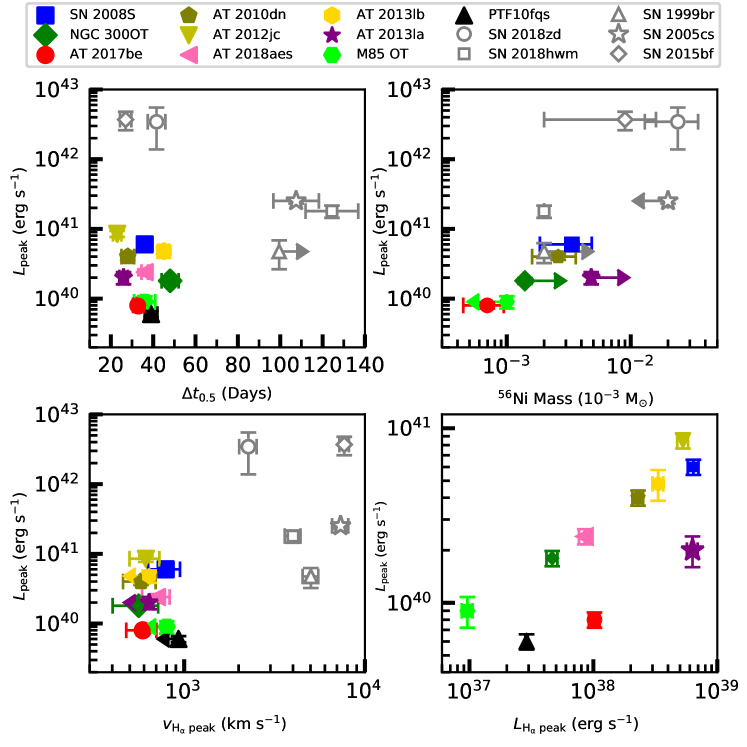
Figure 15: Peak luminosity ($L_{\mathrm{peak}}$) vs. decline time ($\Delta t_{0.5}$) from $L_{\mathrm{peak}}$ to 0.5$L_{\mathrm{peak}}$ (top-left); $L_{\mathrm{peak}}$ vs. ⁵⁶Ni mass (top-right); $L_{\mathrm{peak}}$ vs. $v_{\mathrm{H\alpha}}$ at peak (bottom-left); and $L_{\mathrm{peak}}$ vs. H$\alpha$ peak luminosity (bottom-right).

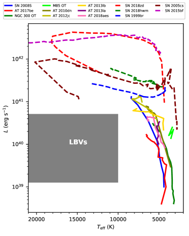
Figure 16: Luminosity ($L$) vs. effective temperature ($T_{\mathrm{eff}}$). ILRTs are marked as solid lines with different colours, while the area where LBVs lie is marked in grey. Comparison SNe II lie in the upper part of the diagram and are labelled with dashed lines.

6.2 Plausible scenarios for ILRTs and conclusions

Although several plausible scenarios have been proposed to explain ILRTs, their nature is still debated. Possible scenarios include LBV-like eruptions, LRN-like events (stellar mergers), and EC-induced SN explosions.

Luminous blue variables originate from massive star ($>$ 20 M_⊙ ) eruptions, and show irregular light curves and SN IIn-like spectra. A luminous progenitor is expected to be detected both in pre-outburst and post-outburst optical and NIR images. No ⁵⁶Ni is expected to be produced. In addition, LBVs and ILRTs are distributed in two separate regions in the $L$-$T_{\rm{eff}}$ diagram (see Figure 16). Our observational arguments disfavour a LBV-like eruption scenario for ILRTs. However, we note that Andrews et al. (2020) proposed that a recent gap transient, AT 2019krl, was an unobscured ILRT eruption from a relatively massive star.

Luminous red novae are another subclass of gap transients, and show double-peaked (or triple-peaked) light curves and a remarkable spectral evolution. Specifically, the major drop in continuum temperature, the appearance of narrow metal lines in absorption, the dramatic change in the H$\alpha$ strength and profile, and the emergence of molecular bands are typical spectral features of LRNe. In addition, the typical H$\alpha$ FWHM velocities of LRNe are lower than 500 $\rm{km}\,s^{-1}$ (Pastorello et al., 2019b). Their colours become progressively redder; for example, the intrinsic $B-V$ colour of an LRN can even reach 1.8 mag at late phases (see Figure 4 of Pastorello et al., 2019b). The evolution of the SED and the radius of LRNe is markedly different from that of ILRTs (Cai et al., 2019; Stritzinger et al., 2020a). LRNe are likely produced by the coalescence of two stars, however we disfavour such a merging scenario for ILRTs.

Theory predicts that some stars with initial mass 8-10 M_⊙  form a S-AGB star with a strongly degenerate oxygen–neon–magnesium (O-Ne-Mg) core surrounded by thin He and H envelopes (e.g. Nomoto, 1984, 1987; Pumo et al., 2009; Takahashi et al., 2013; Moriya et al., 2014; Doherty et al., 2017; Nomoto & Leung, 2017; Leung & Nomoto, 2019; Leung et al., 2020). The final O-Ne-Mg core mass is determined by the competition between core increase from the He and H shell burning and mass loss through thermal pulses (Siess, 2007; Langer, 2012; Leung et al., 2020). Once the core reaches the Chandrasekhar mass (1.37 M_⊙ ; Nomoto, 1984), electron capture reactions on ²⁰Ne and ²⁴Mg take place, and eventually ignite an O-Ne deflagration that propagates outward. This type of CC explosion is referred to as an EC SN (Nomoto, 1984; Zha et al., 2019; Leung et al., 2020). According to models, EC SNe are expected to explode with low energy, low ejected ⁵⁶Ni mass, and typically in a dense and dusty CSM (e.g. Poelarends et al., 2008; Woosley & Heger, 2015; Moriya & Eldridge, 2016). Although Fe-core progenitors at the low-mass end of the CC SNe also explode with low energy ($\sim\leavevmode\nobreak\ 0.5-1.0\times$ 10⁵⁰ erg) and small ⁵⁶Ni mass (4-6 $\times$ 10^-3 M_⊙ ) (Stockinger et al., 2020), some of them (e.g. low-lominosity Type IIP SNe 2003gd, 2005cs, and 2008bk; Eldridge et al., 2007; Maund et al., 2014a, b) can be distinguished from EC SNe through the explosion mechanism, chemical composition, and nucleosynthesis (Jerkstrand et al., 2018). The possible correlations among physical parameters, the homogenous observational properties and the L-T evolution suggest that all ILRTs are regulated by the same mechanism, and the EC SN explosion is a plausible scenario. In particular, this scenario for ILRTs is supported by the following arguments:

• The late-time light curves of SN 2008S and NGC 300 OT2008-1 decline approximately following the ⁵⁶Co decay rate (i.e. $\sim$ 0.98 mag/100d). The ⁵⁶Ni masses inferred from the bolometric light curve are of the order of 10^-4 to 10^-3 M_⊙ , consistent with the expected EC SN yields.
  

• Investigation of archival optical and IR images of the transient locations obtained years before the explosion suggests that the ILRT progenitors are moderately massive, in the range between 8 and 15 M_⊙ . Their progenitors appear to be embedded in dusty cocoons (i.e. SN 2008S; Botticella et al., 2009; Prieto et al., 2009).
  

• Inspection of the transient sites a few years after the explosion suggests that the objects are at least 15 times fainter than the quiescent progenitors (i.e. SN 2008S and NGC 300 OT; Adams et al., 2016). This supports the terminal SN explosion nature.
  

• The estimated ILRT event rate is in fair agreement with EC SN theoretical predictions.

The observational properties described in this paper agree well with theoretical expectations, and we favour terminal EC SN explosions as the possible origin of ILRTs. Future facilities, such as the Vera C. Rubin Observatory and the Nancy Grace Roman Space Telescope, will be essential for expanding the sample of ILRTs, and will be crucial in fine-tuning existing theoretical models.

Appendix A Basic information for observational facilities used

We report the basic information for observational facilities in Table 6, which were used for the five ILRTs.

Table 6: Information on the instrumental setups.

Code	Diameter	Telescope	Instrument	Site
	$\mathrm{m}$
QHY9	0.35	Celestron C14 35-cm reflector	QHY-9	Xingming Observatory, Xinjiang, China
EM01∗	0.40	LCO (FTN site)	EM01	LCO node at Haleakala Observatory, Hawaii, USA
PROMPT3/5	0.41	PROMPT Telescope	Apogee Alta	Cerro Tololo Inter-American Observatory, Cerro Tololo, Chile
TRAPPIST	0.60	TRAPPIST-S Telescope	FLI ProLine	ESO La Silla Observatory, La Silla, Chile
Moravian	0.67/0.92	Schmidt Telescope	Moravian	Osservatorio Astronomico di Asiago, Asiago, Italy
SBIG	0.67/0.92	Schmidt Telescope	SBIG	Osservatorio Astronomico di Asiago, Asiago, Italy
fl03∗	1.00	LCO (LSC site)	Sinistro	LCO node at Cerro Tololo Inter-American Observatory, Cerro Tololo, Chile
fl05∗	1.00	LCO (ELP site)	Sinistro	LCO node at McDonald Observatory, Texas, USA
fl06∗	1.00	LCO (CPT site)	Sinistro	LCO node at South African Astronomical Observatory, Cape Town, South Africa
fl12∗	1.00	LCO (COJ site)	Sinistro	LCO node at Siding Spring Observatory, New South Wales, Australia
B$\&$C	1.22	Galileo Telescope	B$\&$C	Osservatorio Astronomico di Asiago, Asiago, Italy
ANDICAM-CCD	1.30	SMARTS Telescope	ANDICAM	Cerro Tololo Inter-American Observatory, Cerro Tololo, Chile
ANDICAM-IR	1.30	SMARTS Telescope	ANDICAM	Cerro Tololo Inter-American Observatory, Cerro Tololo, Chile
AFOSC	1.82	Copernico Telescope	AFOSC	Osservatorio Astronomico di Asiago, Asiago, Italy
IO:O	2.00	Liverpool Telescope	IO:O	Observatorio Roque de Los Muchachos, La Palma, Spain
RATCam	2.00	Liverpool Telescope	RATCam	Observatorio Roque de Los Muchachos, La Palma, Spain
SupIRCam	2.00	Liverpool Telescope	SupIRCam	Observatorio Roque de Los Muchachos, La Palma, Spain
WFCCD	2.50	Ir$\rm{\acute{e}}$n$\rm{\acute{e}}$e du Pont Telescope	WFCCD	Las Campanas Observatory, Atacama Region, Chile
ALFOSC	2.56	Nordic Optical Telescope	ALFOSC	Observatorio Roque de Los Muchachos, La Palma, Spain
NOTCam	2.56	Nordic Optical Telescope	NOTCam	Observatorio Roque de Los Muchachos, La Palma, Spain
EFOSC2	3.58	New Technology Telescope	EFOSC2	ESO La Silla Observatory, La Silla, Chile
SOFI	3.58	New Technology Telescope	SOFI	ESO La Silla Observatory, La Silla, Chile
LRS	3.58	Telescopio Nazionale Galileo	LRS	Observatorio Roque de Los Muchachos, La Palma, Spain
NICS	3.58	Telescopio Nazionale Galileo	NICS	Observatorio Roque de Los Muchachos, La Palma, Spain
ISIS	4.20	William Hershel Telescope	ISIS	Observatorio Roque de Los Muchachos, La Palma, Spain
LDSS	6.50	Magellan II - Clay Telescope	LDSS	Las Campanas Observatory, Atacama Region, Chile
GMOS	8.10	Gemini South Telescope	GMOS-S	Gemini Observatory, Cerro Pachon, Chile
OSIRIS	10.40	Gran Telescopio CANARIAS	OSIRIS	Observatorio Roque de Los Muchachos, La Palma, Spain

$*$ They are distributed globally at different sites and form part of the LCO global telescope network (Brown et al. 2013).

Appendix B Reddenings and distances adopted for SNe II

In this section, the reddenings and distances adopted for the comparison SNe II are reported in Table 7, along with their respective references.

Table 7: Reddenings and distances of SN 2018zd, SN 2018hwm, SN 2015bf, SN 1999br, and SN 2005cs.

Object	Distance	Distance Modulus	$E(B-V)_{\mathrm{Gal}}$	$E(B-V)_{\mathrm{Host}}$	Sources
	($\mathrm{Mpc}$)	($\mathrm{mag}$)	($\mathrm{mag}$)	($\mathrm{mag}$)	Codes
SN 2018zd	18.4 (4.5)	31.32 (0.48)	0.085	0.085	1
SN 2018hwm	52 (5)	33.58 (0.19)	0.003	0	2
SN 2015bf	60.1 (1.4)	33.89 (0.05)	0.059	0.089	3
SN 1999bra	15.63	30.97	0.021	0	4
SN 2005cs	8.4 (0.5)	29.62 (0.15)	0.031	0.032	5

$Notes$: References for each object are labelled by numbers in the last column. The uncertainties are reported in the parentheses.
1 = Zhang et al. (2020); 2 = Reguitti et al. (2021); 3 = Lin et al. (2021); 4 = Pastorello et al. (2004); 5 = Pastorello et al. (2006).
^a The distance has been rescaled to $H_{0}=73$ $\rm{km}\,s^{-1}$$\rm{Mpc}^{-1}$. The reddening has been updated to the value in Schlafly & Finkbeiner (2011).

Appendix C Photometric data of ILRTs

The photometric data of five ILRTs and associated errors are reported in this section. In addition, black body parameters and SED evolution of individual ILRT AT 2010dn are presented in Table 11 and Figure 17, respectively. Our observations will be made public via the Weizmann Interactive Supernova Data Repository (WISeREP; Yaron & Gal-Yam 2012).

Table 8: Optical ($BVuriz$) photometric measurements of AT 2010dn.

Date	MJD	Phasea	$B$(err)	$V$(err)	$u$(err)	$r$(err)bc	$i$(err)b	$z$(err)	Instrument
20010302	51970.50	-3384.4	–	$>$24.1	–	–	–	–	1
20090330	54921.11	-433.8	–	–	–	$>$19.0	–	–	2
20100521	55338.00	-16.9	–	–	–	$>$18.0	–	–	2
20100531	55348.04	-6.9	–	–	–	17.546(0.123)	–	–	2
20100601	55348.98	-5.9	–	–	–	17.407(0.211)	–	–	2
20100601	55349.45	-5.4	–	–	–	17.593(0.172)	–	–	ALFOSC
20100602	55350.36	-4.5	–	–	–	17.41	–	–	3
20100603	55350.65	-4.2	–	17.4	–	–	–	–	4
20100603	55350.99	-3.9	–	–	–	17.412(0.266)	–	–	2
20100603	55351.40	-3.5	18.036(0.028)	17.649(0.051)	18.780(0.105)	17.465(0.040)	17.379(0.043)	–	LRS
20100605	55352.85	-2.0	17.923(0.036)	17.411(0.044)	18.700(0.206)	17.346(0.040)	17.260(0.036)	17.252(0.065)	EM01
20100607	55355.42	+0.5	17.781(0.046)	17.298(0.047)	18.677(0.080)	17.215(0.060)	17.292(0.040)	–	LRS
20100609	55357.40	+2.5	–	–	–	17.264(0.167)	–	–	ALFOSC
20100611	55359.40	+4.5	18.102(0.034)	17.584(0.017)	–	17.477(0.037)	17.370(0.017)	–	RATCam
20100611	55359.43	+4.5	18.066(0.047)	17.481(0.092)	–	17.424(0.086)	17.347(0.052)	–	LRS
20100612	55360.41	+5.5	18.074(0.016)	17.607(0.029)	–	17.498(0.018)	17.386(0.038)	–	RATCam
20100613	55361.45	+6.6	18.177(0.021)	17.638(0.025)	18.990(0.207)	17.490(0.032)	17.430(0.039)	17.486(0.073)	RATCam
20100616	55363.84	+8.9	18.141(0.053)	17.663(0.031)	19.158(0.358)	17.552(0.034)	17.467(0.038)	17.366(0.048)	EM01
20100616	55364.39	+9.5	–	–	–	17.669(0.248)	–	–	LRS
20100617	55365.40	+10.5	18.139(0.028)	17.730(0.025)	19.237(0.114)	17.605(0.057)	17.495(0.040)	17.376(0.060)	RATCam
20100618	55366.38	+11.5	18.294(0.029)	17.790(0.028)	–	17.607(0.031)	17.486(0.039)	–	RATCam
20100620	55367.82	+12.9	18.261(0.041)	17.701(0.033)	19.233(0.148)	17.700(0.040)	17.442(0.037)	17.378(0.068)	EM01
20100621	55368.79	+13.9	18.325(0.051)	17.752(0.025)	19.186(0.109)	17.650(0.049)	17.550(0.046)	17.432(0.072)	EM01
20100623	55370.80	+15.9	18.367(0.096)	17.797(0.090)	–	17.665(0.048)	17.419(0.072)	17.313(0.088)	EM01
20100623	55371.41	+16.5	18.422(0.022)	17.850(0.033)	19.322(0.137)	17.687(0.049)	17.550(0.039)	17.428(0.056)	RATCam
20100625	55373.41	+18.5	18.449(0.039)	17.907(0.036)	19.405(0.160)	17.619(0.058)	17.504(0.039)	17.445(0.058)	RATCam
20100626	55373.80	+18.9	18.468(0.089)	17.810(0.049)	–	17.667(0.029)	17.574(0.046)	17.395(0.074)	EM01
20100627	55374.80	+19.9	18.489(0.054)	17.930(0.044)	–	17.854(0.047)	17.637(0.043)	17.374(0.073)	EM01
20100628	55375.79	+19.9	–	–	–	–	–	17.465(0.174)	EM01
20100628	55376.39	+21.5	18.699(0.052)	17.934(0.019)	19.612(0.123)	17.828(0.012)	17.558(0.044)	17.473(0.062)	RATCam
20100629	55377.42	+22.5	18.658(0.030)	17.922(0.027)	19.559(0.130)	17.799(0.010)	17.553(0.027)	17.466(0.115)	RATCam
20101117	55517.18	+162.3	22.555(0.101)	22.019(0.040)	–	21.461(0.066)	20.618(0.053)	–	LRS
20101213	55543.08	+188.2	–	22.057(0.116)	–	21.485(0.132)	20.679(0.075)	–	LRS
20101231	55561.20	+206.3	–	22.053(0.149)	–	21.494(0.101)	20.721(0.125)	–	LRS
20110105	55566.14	+211.3	–	–	–	21.542(0.036)	–	–	LRS
20111228	55923.11	+568.2	$>$23.0	$>$22.9	–	$>$22.8	–	–	AFOSC

^a Phases are relative to the $r$-band maximum light: MJD=55354.9.

^b Johnson-Cousins $R$ and $I$ filter data were converted to Sloan $r$ and $i$ band magnitudes respectively, following the relations of Jordi et al. (2006)

^c Unfiltered data obtained by amateur astronomers, calibrated to Sloan $r$-band magnitudes.

$1$ This approximation is based on the similar throughputs between wide filters F555W/F814W and $V$/$I$ . Original data published by Berger (2010), and reported to Johnson-Cousins $V$ and $I$ ($I>$24.9 $\mathrm{mag}$) magnitudes.

$2$ Amateur data (K. Itagaki) scaled to $r$ band .

$3$ Bright Supernova website (http://www.rochesterastronomy.org/sn2010/index.html#2010dn; Observation: J. Nicolas).

$4$ Bright Supernova website (http://www.rochesterastronomy.org/sn2010/index.html#2010dn; Observation: J. Brimacombe).

Table 9: NIR ($JHK$) photometric measurements of AT 2010dn.

Date	MJD	Phasea	$J$(err)	$H$(err)	$K$(err)	Instrument
20100606	55353.89	-1.0	16.611(0.067)	15.690(0.065)	–	SupIRCam
20100607	55354.89	+0.0	16.412(0.133)	15.704(0.053)	15.278(0.068)	NICS
20100607	55354.96	+0.1	16.490(0.091)	15.703(0.119)	–	SupIRCam
20100611	55358.89	+4.0	16.491(0.064)	15.753(0.066)	–	SupIRCam
20100614	55361.90	+7.0	16.564(0.095)	15.830(0.091)	–	SupIRCam
20100627	55374.89	+20.0	16.744(0.340)	15.838(0.082)	–	SupIRCam
20100629	55376.90	+22.0	16.758(0.192)	15.871(0.112)	–	SupIRCam
20101201	55531.22	+176.3	18.974(0.167)	17.774(0.152)	16.868(0.128)	NICS
20101224	55554.14	+199.2	19.341(0.127)	18.053(0.141)	17.465(0.101)	NICS

^a Phases are relative to the $r$-band maximum light: MJD=55354.9.

Table 10: Spitzer IRAC photometry of AT 2010dn (AB mag). Uncertainties are given in parentheses.

Date	MJD	Phasea	CH1 (3.6 $\mu$m)	CH2 (4.5 $\mu$m)
		(d)	(mag)	(mag)
20100708	55385.5	$+30.6$	16.88 (0.01)	16.76 (0.01)
20101230	55560.6	$+205.7$	18.24 (0.03)	17.94 (0.02)
20110203	55595.7	$+240.8$	18.04 (0.03)	17.78 (0.01)
20120114	55940.8	$+585.9$	18.33 (0.03)	18.04 (0.02)
20120616	55094.9	$+740.0$	18.83 (0.05)	18.30 (0.02)
20140130	56687.4	$+1332.5$	21.39 (0.45)	20.09 (0.12)
20140303	56719.1	$+1364.2$	20.99 (0.33)	20.00 (0.11)
20140703	56841.0	$+1486.1$	22.12 (0.76)	20.25 (0.13)
20140706	56844.5	$+1489.6$	21.76 (0.59)	20.24 (0.13)
20150211	57064.9	$+1710.0$	22.44 (0.93)	21.12 (0.28)

^a Phases are relative to the $R/r$-band maximum (MJD=55354.9).

Table 11: Parameters of blackbody fit to the uBVrizJHK bands of AT 2010dn. Uncertainties are given in parentheses.

Date	MJD	Phasea	Luminosity (hot)	Temperature (hot)	Radius (hot)
		(d)	(1039erg s-1)	(K)	(1013 cm)
20100603	55351.40	$-3.5$	66.6 (28.0)	6350 (320)	24.0 (5.1)
20100605	55352.85	$-2.0$	75.5 (10.1)	6405 (100)	25.1 (1.7)
20100607b	55354.89	$0.0$	75.2 (37.5)	6490 (1200)	24.4 (12.2)
20100607	55355.42	$+0.5$	78.8 (34.5)	6460 (360)	25.2 (5.5)
20100611	55358.89	$+4.0$	72.4 (26.9)	6290 (295)	25.5 (4.7)
20100611	55359.40	$+4.5$	69.7 (32.4)	6035 (350)	27.1 (6.3)
20100613	55361.45	$+6.6$	63.7 (17.8)	6075 (200)	25.6 (3.6)
20100617	55365.40	$+10.5$	59.6 (26.2)	6090 (310)	24.6 (5.4)
20100623	55371.41	$+16.5$	54.3 (9.5)	5795 (110)	26.0 (2.3)
20100628	55376.39	$+21.5$	48.8 (10.7)	5390 (135)	28.5 (3.1)
20101117	55517.18	$+162.3$	3.5 (5.1)	3380 (420)	19.3 (14.2)
20101201b	55531.22	$176.3$	3.2 (1.6)	3420 (170)	18.2 (9.1)
20101224b	55554.14	$199.2$	2.8 (1.4)	3540 (280)	15.9 (8.0)

^a Phases are relative to the $r$-band maximum light curve (MJD=55354.9).
^b Data are obtained by fitting a double black body function, but only the first hot-component parameters are reported. The second warm component has large uncertainties because its data are incompletely sampled.

Table 12: Optical ($UBVRI$) photometric measurements of AT 2012jc.

Date	MJD	Phasea	$U$(err)	$B$(err)	$V$(err)	$R$(err)	$I$(err)	Instrument
20120313	55999.27	-24.2	–	–	–	$>$19.9	–	PROMPT3/5b
20120317	56003.39	-20.1	–	–	$>$19.5	–	–	1
20120327	56013.49	-10.0	–	–	18.7	–	–	1
20120328	56014.07	-9.4	–	–	18.5	–	–	1
20120329	56015.06	-8.4	20.308(0.114)	18.823(0.022)	18.206 (0.027)	17.855 (0.031)	17.460 (0.058)	RATCam
20120329	56015.14	-8.4	–	18.744(0.053)	18.259 (0.044)	17.924 (0.034)	17.521 (0.129)	AFOSC
20120329	56015.35	-8.2	–	–	18.0 (0.1)	–	–	2
20120331	56017.26	-6.2	–	18.390(0.113)	17.888 (0.051)	17.503 (0.064)	17.129 (0.056)	PROMPT3
20120412	56029.24	+5.7	–	–	17.776 (0.069)	17.403 (0.057)	17.102 (0.045)	PROMPT3/5
20120414	56031.37	+7.9	–	18.422(0.020)	17.901 (0.020)	17.564 (0.013)	17.164 (0.029)	EFOSC2
20120415	56032.41	+8.9	–	–	–	17.614 (0.062)	–	PROMPT3/5
20120416	56033.24	+9.7	–	–	17.904 (0.055)	17.561 (0.059)	17.239 (0.049)	PROMPT3/5
20120416	56033.97	+10.5	19.391(0.093)	18.494(0.028)	17.902 (0.029)	17.552 (0.032)	17.285 (0.112)	RATCam
20120417	56034.05	+10.6	–	18.443(0.034)	17.947 (0.030)	17.591 (0.017)	17.287 (0.055)	AFOSC
20120417	56034.19	+10.7	–	–	17.900 (0.069)	17.634 (0.056)	17.201 (0.067)	PROMPT3/5
20120421	56038.25	+14.8	–	18.694(0.062)	18.064 (0.049)	17.825 (0.084)	17.445 (0.057)	PROMPT3/5
20120422	56039.01	+15.5	19.917(0.109)	18.598(0.024)	18.117 (0.025)	17.856 (0.031)	17.511 (0.053)	RATCam
20120425	56042.11	+18.6	–	–	18.478 (0.109)	18.094 (0.168)	17.710 (0.126)	SBIG
20120501	56048.17	+24.7	–	19.011(0.084)	18.436 (0.080)	18.083 (0.055)	17.649 (0.071)	PROMPT3/5
20120501	56048.20	+24.7	–	19.155(0.013)	18.479 (0.018)	–	–	ALFOSC
20120501	56048.38	+24.9	–	19.064(0.031)	18.487 (0.032)	18.112 (0.029)	17.696 (0.074)	EFOSC2
20120502	56049.21	+25.7	–	19.134(0.113)	18.485 (0.088)	18.073 (0.058)	17.647 (0.094)	PROMPT3/5
20120509	56056.10	+32.6	–	19.386(0.033)	18.595 (0.035)	18.154 (0.076)	17.700 (0.088)	LRS
20120515	56062.11	+38.6	21.101(0.212)	19.560(0.039)	18.743 (0.044)	18.292 (0.050)	17.701 (0.226)	RATCam
20120515	56062.24	+38.7	–	–	18.707 (0.068)	18.226 (0.072)	17.647 (0.042)	PROMPT3/5
20120520	56067.18	+43.7	–	–	–	–	17.788 (0.052)	PROMPT3/5
20120521	56068.17	+44.7	–	19.710(0.132)	18.807 (0.068)	18.325 (0.078)	17.819 (0.035)	PROMPT3/5
20120601	56079.97	+56.5	$>$21.3	20.142(0.111)	19.217 (0.051)	18.699 (0.058)	18.089 (0.057)	RATCam
20120603	56081.11	+57.6	–	–	–	18.804 (0.154)	–	PROMPT3/5b
20120603	56081.96	+58.5	$>$21.3	20.196(0.148)	19.263 (0.093)	18.741 (0.040)	18.115 (0.079)	RATCam
20120620	56098.24	+74.7	–	20.501(0.148)	19.512 (0.101)	$>$19.7	–	TRAPPIST

^a Phases are relative to the $R$-band maximum light: MJD=56023.5.

^b These unfiltered data were reported to Johnson-Cousins $R$ magnitudes, as suggested by the quantum efficiency of the CCD.

$1$ Observations from The Astronomer’s Telegram (ATel, No. 4004; see Howerton et al. 2012).

$2$ Bright Supernova website (http://www.rochesterastronomy.org/sn2012/index.html#PSNJ14535395+0334049; Observation: J. Brimacombe)

Table 13: Optical ($UBVRI$) photometric measurements of AT 2013lb.

Date	MJD	Phasea	$U$(err)	$B$(err)	$V$(err)	$R$(err)	$I$(err)	Instrument
20120624	56102.05	-222.4	–	–	–	$>$19.2	–	PROMPT35b
20130127	56319.34	-5.2	–	–	–	18.897(0.138)	–	PROMPT35b
20130131	56323.34	-1.2	–	–	–	18.728(0.099)	–	PROMPT35b
20130204	56327.36	+2.9	–	–	–	18.601(0.143)	–	PROMPT35b
20130204	56327.41	+2.9	–	–	–	$>$18.3	–	1
20130207	56330.20	+5.7	–	–	19.132(0.144)	18.833(0.078)	18.422(0.090)	AFOSC
20130207	56330.39	+5.9	–	–	19.143(0.035)	–	–	EFOSC2
20130208	56331.23	+6.7	–	–	–	18.859(0.029)	18.450(0.038)	RATCam
20130209	56332.28	+7.8	–	–	19.237(0.035)	–	–	EFOSC2
20130211	56334.23	+9.7	–	–	–	18.998(0.030)	18.466(0.035)	RATCam
20130215	56338.28	+13.8	–	19.878(0.046)	19.368(0.029)	18.882(0.043)	18.455(0.064)	ANDICAM-CCD
20130218	56341.23	+16.7	19.541(0.160)	19.997(0.060)	–	19.005(0.037)	18.415(0.038)	RATCam
20130218	56341.32	+16.8	–	19.963(0.047)	19.444(0.034)	18.888(0.062)	18.346(0.068)	ANDICAM-CCD
20130220	56343.30	+18.8	–	19.937(0.042)	19.350(0.031)	19.050(0.031)	18.474(0.042)	ANDICAM-CCD
20130221	56344.22	+19.7	$>$19.9	19.998(0.046)	19.307(0.034)	18.987(0.050)	18.455(0.040)	RATCam
20130223	56346.20	+21.7	$>$19.9	20.084(0.110)	19.413(0.046)	18.937(0.078)	18.458(0.064)	RATCam
20130225	56348.14	+23.6	$>$19.9	20.188(0.178)	19.385(0.082)	19.001(0.088)	18.550(0.075)	RATCam
20130227	56350.30	+25.8	–	20.226(0.124)	19.510(0.093)	–	–	ANDICAM-CCD
20130301	56352.32	+27.8	–	–	–	19.111(0.071)	18.695(0.087)	ANDICAM-CCD
20130305	56356.25	+31.8	–	–	–	19.113(0.054)	–	EFOSC2b
20130305	56356.26	+31.8	–	20.367(0.077)	19.616(0.056)	19.167(0.045)	18.558(0.065)	ANDICAM-CCD
20130310	56361.22	+36.7	–	$>$20.4	$>$19.6	19.115(0.226)	18.496(0.293)	RATCam
20130311	56362.26	+37.8	–	20.509(0.052)	19.618(0.052)	19.076(0.050)	18.594(0.063)	ANDICAM-CCD
20130312	56363.09	+38.6	$>$19.9	20.590(0.080)	19.688(0.051)	19.143(0.054)	18.625(0.051)	RATCam
20130315	56366.28	+41.8	–	20.689(0.051)	19.857(0.057)	19.082(0.038)	18.755(0.043)	ANDICAM-CCD
20130318	56369.07	+44.6	$>$20.0	20.850(0.138)	19.802(0.071)	19.284(0.075)	18.675(0.090)	RATCam
20130320	56371.33	+46.8	–	20.949(0.060)	19.984(0.063)	19.257(0.030)	18.735(0.084)	ANDICAM-CCD
20130321	56372.11	+47.6	$>$20.1	20.921(0.088)	19.991(0.049)	19.295(0.067)	18.721(0.057)	RATCam
20130324	56375.29	+50.8	–	21.018(0.120)	20.111(0.094)	19.484(0.056)	18.634(0.071)	ANDICAM-CCD
20130328	56379.26	+54.8	–	21.277(0.358)	19.913(0.131)	19.469(0.159)	18.610(0.125)	ANDICAM-CCD
20130401	56383.12	+58.6	–	$>$21.2	20.089(0.195)	19.386(0.202)	18.656(0.130)	RATCam
20130407	56389.07	+64.6	–	21.584(0.195)	20.280(0.083)	19.682(0.085)	19.049(0.059)	RATCam
20130409	56392.00	+67.5	–	21.746(0.225)	20.476(0.097)	19.863(0.104)	18.963(0.102)	RATCam
20130414	56396.30	+71.8	–	21.839(0.028)	20.794(0.046)	20.054(0.037)	19.391(0.063)	EFOSC2
20150214	57067.31	+742.8	–	–	–	$>$19.8	–	PROMPT35b

^a Phases are relative to the $R$-band maximum light: MJD=56324.5.

^b Unfiltered data reported to broad-band Johnson-Cousins $R$ magnitudes.

$1$ This limit was obtained by L. Elenin (Lyubertsy, Russia) and I. Molotov (Moscow, Russia) through a 0.45-m f/2.8 telescope plus KAF09000 CCD, which is also reported in the Central Bureau for Astronomical Telegrams (CBAT, see http://www.cbat.eps.harvard.edu/unconf/followups/J15213475-0722183.html).

Table 14: NIR ($JHK$) photometric measurements of AT 2013lb.

Date	MJD	Phasea	$J$(err)	$H$(err)	$K$(err)	Instrument
20130208	56331.29	+6.8	17.700(0.038)	17.239(0.039)	16.761(0.047)	SOFI
20130218	56341.30	+16.8	17.967(0.165)	–	–	ANDICAM-IR
20130220	56343.29	+18.8	17.988(0.184)	–	–	ANDICAM-IR
20130222	56345.36	+20.9	17.977(0.096)	17.339(0.039)	16.975(0.052)	SOFI
20130227	56350.29	+25.8	17.947(0.161)	–	–	ANDICAM-IR
20130301	56352.30	+27.8	17.936(0.179)	–	–	ANDICAM-IR
20130305	56356.25	+31.8	18.036(0.145)	–	–	ANDICAM-IR
20130306	56357.31	+32.8	18.002(0.096)	17.505(0.101)	16.981(0.060)	SOFI
20130311	56362.25	+37.8	18.137(0.205)	–	–	ANDICAM-IR
20130315	56366.27	+41.8	18.070(0.135)	–	–	ANDICAM-IR
20130320	56371.32	+46.8	18.004(0.153)	–	–	ANDICAM-IR
20130324	56375.27	+50.8	18.068(0.136)	–	–	ANDICAM-IR
20130328	56379.25	+54.8	18.182(0.215)	–	–	ANDICAM-IR
20130412	56394.33	+69.8	18.292(0.081)	17.705(0.067)	17.362(0.065)	SOFI

^a Phases are relative to the $R$-band maximum light: MJD=56324.5.

Table 15: Optical ($BVugriz$) photometric measurements of AT 2013la.

Date	MJD	Phasea	$B$(err)	$V$(err)	$u$(err)	$g$(err)	$r$(err)b	$i$(err)b	Instrument
20130331	56382.71	-269.3	–	–	–	–	$>$18.8	–	QHY9c
20131220	56646.93	-5.4	–	–	–	–	18.246(0.251)	–	QHY9c
20131226	56652.96	+1.0	–	–	–	–	17.992(0.230)	–	QHY9c
20131227	56653.93	+1.9	–	–	–	–	17.964(0.180)	–	QHY9c
20131229	56655.87	+3.9	–	–	–	–	18.062(0.165)	–	QHY9c
20131230	56656.87	+4.9	–	–	–	–	$>$17.8	–	QHY9c
20140101	56658.21	+6.2	19.393(0.035)	18.634(0.013)	20.840(0.186)	–	18.314(0.011)	18.101(0.010)	IO:O
20140102	56659.16	+7.2	19.386(0.045)	18.691(0.030)	20.519(0.218)	–	18.351(0.015)	18.133(0.016)	IO:O
20140104	56661.26	+9.3	19.373(0.045)	18.702(0.014)	20.227(0.136)	–	18.360(0.013)	18.202(0.012)	IO:O
20140107	56664.26	+12.3	19.522(0.034)	18.763(0.051)	20.160(0.108)	–	18.490(0.039)	18.293(0.121)	IO:O
20140107	56664.84	+12.8	–	–	–	–	18.467(0.396)	–	QHY9c
20140108	56665.16	+13.2	19.432(0.112)	18.774(0.055)	$>$19.6	–	18.511(0.069)	18.208(0.044)	IO:O
20140108	56665.23	+13.2	–	18.811(0.180)	–	–	18.417(0.218)	–	AFOSC
20140109	56666.96	+15.0	–	–	–	–	18.501(0.224)	–	QHY9c
20140111	56668.88	+16.9	–	–	–	–	18.529(0.213)	–	QHY9c
20140115	56672.15	+21.1	19.559(0.066)	18.888(0.073)	20.093(0.211)	–	18.555(0.028)	18.404(0.022)	IO:O
20140122	56679.14	+27.1	19.650(0.085)	19.083(0.058)	–	–	18.636(0.256)	18.672(0.058)	SBIG
20140127	56684.27	+32.3	19.957(0.042)	19.154(0.026)	–	–	18.803(0.022)	18.751(0.028)	IO:O
20140204	56692.23	+40.2	–	–	–	–	19.111(0.008)	–	LRS
20140207	56695.24	+43.2	20.223(0.037)	19.357(0.022)	20.386(0.186)	–	19.030(0.019)	18.985(0.023)	IO:O
20140209	56697.61	+45.6	–	–	–	20.06	–	–	1
20140209	56697.62	+45.6	–	–	–	20.13	–	–	1d
20140210	56698.24	+46.2	20.187(0.038)	19.480(0.032)	20.485(0.150)	–	19.037(0.018)	19.002(0.027)	IO:O
20140213	56701.10	+49.1	20.213(0.093)	19.556(0.050)	–	–	19.054(0.037)	19.086(0.033)	IO:O
20140221	56709.60	+57.6	–	–	–	–	19.14	–	1
20140221	56709.61	+57.6	–	–	–	–	19.22	–	1
20140223	56711.22	+59.2	20.350(0.051)	19.607(0.029)	–	–	19.205(0.022)	19.244(0.027)	IO:O
20140226	56714.28	+62.3	–	–	–	–	19.263(0.017)	19.258(0.038)	OSIRIS
20140228	56716.19	+64.2	20.550(0.054)	19.653(0.033)	$>$20.6	–	19.277(0.022)	19.306(0.039)	IO:O
20140309	56725.17	+73.2	20.603(0.238)	19.923(0.104)	–	–	19.535(0.104)	19.389(0.049)	AFOSC
20140323	56739.10	+87.1	21.051(0.038)	20.250(0.061)	–	–	19.644(0.008)	19.781(0.010)	LRS
20140401	56748.08	+96.1	21.267(0.158)	20.291(0.219)	–	–	–	19.934(0.032)	AFOSC
20140425	56772.99	+121.0	–	20.697(0.023)	–	–	19.838(0.012)	20.107(0.019)	ALFOSC
20140428	56775.94	+123.9	–	–	–	–	19.849(0.080)	20.173(0.085)	OSIRIS
20140514	56791.93	+139.9	–	20.985(0.086)	–	–	19.927(0.039)	20.357(0.064)	LRS
20140615	56823.94	+171.9	21.713(0.048)	21.340(0.033)	–	–	20.151(0.015)	20.545(0.017)	LRS
20140723	56861.92	+209.9	21.949(0.054)	21.454(0.035)	–	–	20.310(0.013)	20.619(0.023)	LRS
20140808	56877.88	+225.9	22.257(0.070)	21.693(0.047)	–	–	20.447(0.020)	20.816(0.025)	LRS
20140814	56883.88	+231.9	–	–	–	–	20.540(0.165)	20.925(0.046)	OSIRIS
20141217	57008.20	+356.2	–	–	–	–	21.531(0.106)	–	ALFOSC
20141220	57011.19	+359.2	–	22.302(0.539)	–	–	21.406(0.106)	21.540(0.196)	AFOSC
20141223	57014.25	+362.2	–	–	–	–	21.450(0.168)	21.612(0.124)	OSIRIS
20150125	57047.27	+395.3	–	$>$22.5	–	–	21.815(0.034)	21.967(0.041)	ALFOSC
20150311	57092.27	+440.3	–	$>$22.6	–	–	22.436(0.070)	–	ALFOSC
20150428	57140.77	+488.8	–	–	–	–	$>$23.0	–	ALFOSC

^a Phases are relative to the $r$-band maximum light: MJD=56652.0.

^b Johnson-Cousins $R$ and $I$ filter data were transformed to Sloan $r$ and $i$ band magnitudes respectively, following the relations of Jordi et al. (2006)

^c Measurements on unfiltered images, calibrated to the Sloan $r$-band magnitudes.

^d This epoch also has a $z$-band detection at 18.69 $\mathrm{mag}$. In addition, there is a very early (2013-03-07; MJD=56476.29) $z$-band limit of $>$ 20.8 mag.

$1$ These data were taken from the Pan-STARRS Survey for Transients (see website:

https://star.pst.qub.ac.uk/ps1threepi/psdb/candidate/1131007351341051000/).

Table 16: Optical ($BVgriz$) photometric measurements of AT 2018aes.

Date	MJD	Phasea	$B$(err)	$V$(err)	$g$(err)	$r$(err)	$i$(err)	$z$(err)	Instrument
20180215	58164.65	-46.5	–	–	–	$>$20.1	–	–	ATLAS∗
20180218	58167.57	-43.5	–	–	–	$>$18.7	–	–	1
20180307	58184.61	-26.5	–	–	–	$>$20.1	–	–	ATLAS
20180311	58188.54	-22.6	–	–	–	18.51(0.3)	–	–	1
20180311	58188.55	-22.6	–	–	–	–	19.103(0.029)	–	2
20180311	58188.61	-22.5	–	–	–	19.21(0.60)	–	–	ATLAS
20180314	58191.73	-19.4	20.004(0.089)	19.321(0.084)	19.613(0.054)	19.051(0.061)	18.881(0.103)	–	fl12
20180317	58194.59	-16.5	–	–	19.52(0.44)	–	–	–	ATLAS
20180318	58195.09	-16.0	19.794(0.074)	19.185(0.084)	19.558(0.021)	18.997(0.052)	18.727(0.080)	–	fl06
20180319	58196.59	-14.5	–	–	–	18.78(0.34)	–	–	ATLAS
20180322	58199.12	-12.0	19.841(0.027)	19.140(0.020)	19.509(0.011)	18.949(0.023)	18.896(0.023)	–	ALFOSC
20180322	58199.38	-11.7	19.868(0.131)	19.082(0.078)	19.402(0.047)	18.919(0.061)	18.775(0.080)	–	fl05
20180326	58203.23	-7.9	$>$19.6	18.904(0.064)	19.314(0.045)	18.830(0.048)	18.663(0.072)	–	fl03
20180329	58206.50	-4.6	–	–	–	18.84(0.31)	–	–	ATLAS
20180330	58207.11	-4.0	19.714(0.068)	19.089(0.065)	19.383(0.064)	18.827(0.045)	18.716(0.041)	18.634(0.075)	ALFOSC
20180405	58213.09	+2.0	19.830(0.020)	19.019(0.010)	19.386(0.010)	18.858(0.010)	18.546(0.049)	18.569(0.027)	ALFOSC
20180407	58215.19	+4.1	–	19.069(0.026)	19.465(0.031)	18.750(0.050)	18.575(0.027)	18.479(0.045)	ALFOSC
20180408	58216.16	+5.1	19.923(0.029)	19.068(0.019)	19.486(0.010)	18.871(0.015)	18.652(0.025)	18.605(0.041)	ALFOSC
20180411	58219.14	+8.0	19.934(0.025)	19.011(0.011)	19.559(0.010)	18.876(0.019)	18.632(0.030)	18.596(0.035)	ALFOSC
20180412	58220.53	+9.4	–	–	–	18.77(0.10)	–	–	ATLAS
20180417	58225.03	+13.9	20.104(0.042)	19.220(0.024)	19.590(0.025)	18.952(0.024)	18.725(0.018)	18.574(0.037)	ALFOSC
20180418	58226.10	+15.0	20.184(0.075)	19.224(0.029)	19.653(0.018)	19.021(0.022)	18.773(0.040)	18.758(0.051)	IO:O
20180418	58226.98	+15.9	–	19.138(0.104)	19.648(0.094)	19.039(0.078)	19.005(0.135)	–	Moravian
20180419	58227.98	+16.9	20.121(0.175)	19.205(0.088)	19.736(0.090)	18.969(0.099)	18.811(0.219)	–	Moravian
20180426	58234.13	+23.0	20.389(0.033)	19.563(0.017)	19.885(0.025)	19.172(0.021)	18.899(0.038)	18.785(0.043)	ALFOSC
20180501	58239.04	+27.9	20.584(0.049)	19.570(0.022)	20.099(0.019)	19.390(0.043)	19.089(0.032)	19.033(0.046)	ALFOSC
20180504	58242.98	+31.9	20.771(0.134)	19.654(0.050)	20.124(0.054)	19.476(0.031)	19.200(0.050)	18.999(0.078)	IO:O
20180507	58245.98	+34.9	20.820(0.104)	19.781(0.028)	20.478(0.033)	19.538(0.013)	19.313(0.061)	19.021(0.090)	IO:O
20180510	58248.48	+37.4	–	–	–	19.66(0.62)	–	–	ATLAS
20180513	58251.02	+39.9	21.111(0.146)	20.175(0.043)	20.566(0.065)	19.798(0.041)	19.568(0.082)	19.145(0.068)	IO:O
20180515	58254.00	+42.9	21.182(0.086)	20.189(0.041)	20.693(0.041)	19.938(0.036)	19.473(0.037)	19.181(0.044)	ALFOSC
20180517	58255.95	+44.8	21.239(0.210)	20.276(0.080)	20.972(0.051)	20.008(0.039)	19.651(0.121)	19.313(0.070)	IO:O
20180522	58260.92	+49.8	$>$21.2	20.468(0.120)	21.261(0.373)	20.140(0.087)	19.985(0.116)	19.498(0.118)	IO:O
20180525	58263.05	+52.0	21.714(0.111)	20.559(0.105)	21.343(0.046)	20.356(0.071)	20.092(0.082)	19.728(0.071)	ALFOSC
20180531	58269.02	+57.9	22.048(0.164)	20.986(0.060)	21.813(0.062)	20.608(0.024)	20.257(0.121)	19.910(0.093)	ALFOSC
20180531	58269.94	+58.8	$>$21.8	$>$20.9	$>$21.6	$>$20.7	20.332(0.275)	19.900(0.267)	IO:O
20180605	58274.05	+62.9	22.189(0.128)	21.106(0.070)	21.898(0.073)	20.907(0.032)	20.567(0.114)	19.917(0.060)	ALFOSC
20180605	58274.91	+63.8	$>$21.8	21.280(0.075)	21.956(0.120)	20.831(0.044)	20.708(0.435)	19.911(0.161)	IO:O
20180610	58279.99	+68.9	$>$21.8	21.454(0.193)	22.124(0.147)	21.304(0.123)	20.712(0.258)	20.258(0.235)	IO:O
20180626	58295.97	+84.9	–	–	$>$22.5	22.335(0.104)	$>$21.8	20.996(0.226)	ALFOSC
20180704	58303.97	+92.9	–	–	–	22.865(0.221)	21.866(0.379)	21.414(0.211)	ALFOSC

^a Phases are relative to the $r$-band maximum light: MJD= 58211.1.

^∗ ATLAS (Asteroid Terrestrial-impact Last Alert System; Heinze et al. 2018; Tonry et al. 2018; Smith et al. 2020) observations in cyan- and orange-band magnitudes are reported in the sloan g and r columns respectively.

$1$ Unfiltered KAIT data reported to the sloan $r$ magnitudes (AB system). Data from the Transient Name Server (TNS; https://wis-tns.weizmann.ac.il/object/2018aes).

$2$ The $i$-band magnitude is the weighted mean value obtained from the Pan-STARRS Survey for Transients (see website: https://star.pst.qub.ac.uk/sne/ps13pi/psdb/lightcurve/1134817771035644300/).

Table 17: NIR ($JHK$) photometric measurements of AT 2018aes.

Date	MJD	Phasea	$J$(err)	$H$(err)	$K$(err)	Instrument
20180331	58209.00	-2.1	17.781(0.040)	17.387(0.075)	16.235(0.088)	NOTCam
20180511	58249.92	+38.8	18.257(0.065)	17.994(0.063)	17.148(0.076)	NOTCam
20180627	58296.95	+85.9	19.752(0.209)	19.363(0.299)	17.957(0.160)	NOTCam
20180731	58330.88	+119.8	$>$ 20.5	19.662(0.392)	–	NOTCam
20180819	58349.86	+138.8	–	–	18.442(0.186)	NOTCam

^a Phases are relative to the $r$-band maximum light: MJD= 58211.1.

References

- Adams et al. (2018) Adams, S. M., Blagorodnova, N., Kasliwal, M. M., et al. 2018, PASP, 130, 034202
- Adams et al. (2016) Adams, S. M., Kochanek, C. S., Prieto, J. L., et al. 2016, MNRAS, 460, 1645
- Albareti et al. (2017) Albareti, F. D., Allende Prieto, C., Almeida, A., et al. 2017, ApJS, 233, 25
- Andretta et al. (2005) Andretta, V., Busà, I., Gomez, M. T., & Terranegra, L. 2005, A&A, 430, 669
- Andrews et al. (2018) Andrews, J., Smith, N., & Van Dyk, S. D. 2018, The Astronomer’s Telegram, 11441, 1
- Andrews et al. (2011) Andrews, J. E., Clayton, G. C., Wesson, R., et al. 2011, AJ, 142, 45
- Andrews et al. (2020) Andrews, J. E., Jencson, J. E., Van Dyk, S. D., et al. 2020, arXiv e-prints, arXiv:2009.13541
- Arcavi et al. (2018) Arcavi, I., Hosseinzadeh, G., Hiramatsu, D., et al. 2018, Transient Name Server Classification Report, 2018-2082, 1
- Arnett & Fu (1989) Arnett, W. D. & Fu, A. 1989, ApJ, 340, 396
- Asplund et al. (2009) Asplund, M., Grevesse, N., Sauval, A. J., & Scott, P. 2009, ARA&A, 47, 481
- Barsukova et al. (2014) Barsukova, E. A., Goranskij, V. P., Valeev, A. F., & Kaisin, S. S. 2014, Variable Stars
- Becker (2015) Becker, A. 2015, HOTPANTS: High Order Transform of PSF ANd Template Subtraction
- Berger (2010) Berger, E. 2010, The Astronomer’s Telegram, 2655
- Berger et al. (2012) Berger, E., Marion, G. H., Hsiao, E., Foley, R., & Chornock, R. 2012, The Astronomer’s Telegram, 4009
- Berger et al. (2009a) Berger, E., Roth, K., Stubbs, C., et al. 2009a, Exotic Explosions and Eruptions: Exploring a New Transient Phase-Space with Pan-STARRS, NOAO Proposal
- Berger et al. (2009b) Berger, E., Soderberg, A. M., Chevalier, R. A., et al. 2009b, ApJ, 699, 1850
- Bertin & Arnouts (1996) Bertin, E. & Arnouts, S. 1996, A&AS, 117, 393
- Blagorodnova et al. (2017) Blagorodnova, N., Kotak, R., Polshaw, J., et al. 2017, ApJ, 834, 107
- Bond et al. (2009) Bond, H. E., Bedin, L. R., Bonanos, A. Z., et al. 2009, ApJ, 695, L154
- Botticella et al. (2009) Botticella, M. T., Pastorello, A., Smartt, S. J., et al. 2009, MNRAS, 398, 1041
- Bouchet et al. (1991) Bouchet, P., Danziger, I. J., & Lucy, L. B. 1991, AJ, 102, 1135
- Brown et al. (2013) Brown, T. M., Baliber, N., Bianco, F. B., et al. 2013, PASP, 125, 1031
- Burke et al. (2019) Burke, J., Howell, D. A., Arcavi, I., et al. 2019, Transient Name Server Classification Report, 2019-328, 1
- Busà et al. (2007) Busà, I., Aznar Cuadrado, R., Terranegra, L., Andretta, V., & Gomez, M. T. 2007, A&A, 466, 1089
- Cai et al. (2018) Cai, Y.-Z., Pastorello, A., Fraser, M., et al. 2018, MNRAS, 480, 3424
- Cai et al. (2019) Cai, Y. Z., Pastorello, A., Fraser, M., et al. 2019, A&A, 632, L6
- Cardelli et al. (1989) Cardelli, J. A., Clayton, G. C., & Mathis, J. S. 1989, ApJ, 345, 245
- Catchpole et al. (1988) Catchpole, R. M., Whitelock, P. A., Feast, M. W., et al. 1988, MNRAS, 231, 75p
- Catchpole et al. (1989) Catchpole, R. M., Whitelock, P. A., Menzies, J. W., et al. 1989, MNRAS, 237, 55P
- Chevalier & Fransson (1994) Chevalier, R. A. & Fransson, C. 1994, ApJ, 420, 268
- Chonis & Gaskell (2008) Chonis, T. S. & Gaskell, C. M. 2008, AJ, 135, 264
- Corwin et al. (1994) Corwin, Harold G., J., Buta, R. J., & de Vaucouleurs, G. 1994, AJ, 108, 2128
- De et al. (2019) De, K., Tartaglia, L., Andreoni, I., et al. 2019, The Astronomer’s Telegram, 12433, 1
- de Groot (1969a) de Groot, M. 1969a, Bull. Astron. Inst. Netherlands, 20, 225
- de Groot (1969b) de Groot, M. 1969b, Commmunications of the Konkoly Observatory Hungary, 65, 203
- de Vaucouleurs et al. (1991) de Vaucouleurs, G., de Vaucouleurs, A., Corwin, Herold G., J., et al. 1991, Third Reference Catalogue of Bright Galaxies
- Doherty et al. (2017) Doherty, C. L., Gil-Pons, P., Siess, L., & Lattanzio, J. C. 2017, PASA, 34, e056
- Doherty et al. (2015) Doherty, C. L., Gil-Pons, P., Siess, L., Lattanzio, J. C., & Lau, H. H. B. 2015, MNRAS, 446, 2599
- Eastman et al. (1994) Eastman, R. G., Woosley, S. E., Weaver, T. A., & Pinto, P. A. 1994, ApJ, 430, 300
- Eldridge et al. (2007) Eldridge, J. J., Mattila, S., & Smartt, S. J. 2007, MNRAS, 376, L52
- Ferrarese et al. (2000) Ferrarese, L., Mould, J. R., Kennicutt, Jr., R. C., et al. 2000, ApJ, 529, 745
- Filippenko (1997) Filippenko, A. V. 1997, ARA&A, 35, 309
- Fransson et al. (2014) Fransson, C., Ergon, M., Challis, P. J., et al. 2014, ApJ, 797, 118
- Fremling et al. (2019) Fremling, C., Dugas, A., & Sharma, Y. 2019, Transient Name Server Classification Report, 2019-2789, 1
- Gerardy et al. (2002) Gerardy, C. L., Fesen, R. A., Nomoto, K., et al. 2002, ApJ, 575, 1007
- Grassberg et al. (1971) Grassberg, E. K., Imshennik, V. S., & Nadyozhin, D. K. 1971, Ap&SS, 10, 28
- Hamuy (2003) Hamuy, M. 2003, ApJ, 582, 905
- Hamuy (2001) Hamuy, M. A. 2001, PhD thesis, The University of Arizona
- Heinze et al. (2018) Heinze, A. N., Tonry, J. L., Denneau, L., et al. 2018, AJ, 156, 241
- Hiramatsu et al. (2021) Hiramatsu, D., Howell, D. A., Van Dyk, S. D., et al. 2021, Nature Astronomy
- Howerton et al. (2012) Howerton, S., Prieto, J., Drake, A. J., et al. 2012, The Astronomer’s Telegram, 4004
- Humphreys et al. (2011) Humphreys, R. M., Bond, H. E., Bedin, L. R., et al. 2011, ApJ, 743, 118
- Humphreys & Davidson (1994) Humphreys, R. M. & Davidson, K. 1994, PASP, 106, 1025
- Humphreys et al. (1999) Humphreys, R. M., Davidson, K., & Smith, N. 1999, PASP, 111, 1124
- Jencson et al. (2019) Jencson, J. E., Adams, S. M., Bond, H. E., et al. 2019, ApJ, 880, L20
- Jerkstrand et al. (2018) Jerkstrand, A., Ertl, T., Janka, H. T., et al. 2018, MNRAS, 475, 277
- Jha (2019) Jha, S. 2019, Transient Name Server Classification Report, 2019-1237, 1
- Jha et al. (2019) Jha, S. W., Eweis, Y., Camacho-Neves, Y., et al. 2019, The Astronomer’s Telegram, 12454, 1
- Jordi et al. (2006) Jordi, K., Grebel, E. K., & Ammon, K. 2006, A&A, 460, 339
- Kashi et al. (2010) Kashi, A., Frankowski, A., & Soker, N. 2010, ApJ, 709, L11
- Kasliwal (2012) Kasliwal, M. M. 2012, PASA, 29, 482
- Kasliwal et al. (2011) Kasliwal, M. M., Kulkarni, S. R., Arcavi, I., et al. 2011, ApJ, 730, 134
- Kitaura et al. (2006) Kitaura, F. S., Janka, H. T., & Hillebrandt, W. 2006, A&A, 450, 345
- Kochanek (2011) Kochanek, C. S. 2011, ApJ, 741, 37
- Kochanek et al. (2014) Kochanek, C. S., Adams, S. M., & Belczynski, K. 2014, MNRAS, 443, 1319
- Kozyreva et al. (2021) Kozyreva, A., Baklanov, P., Jones, S., Stockinger, G., & Janka, H.-T. 2021, MNRAS, 503, 797
- Kulkarni & Kasliwal (2009) Kulkarni, S. & Kasliwal, M. M. 2009, in Astrophysics with All-Sky X-Ray Observations, ed. N. Kawai, T. Mihara, M. Kohama, & M. Suzuki, 312
- Kulkarni et al. (2007) Kulkarni, S. R., Ofek, E. O., Rau, A., et al. 2007, Nature, 447, 458
- Lambert et al. (1969) Lambert, D. L., Mallia, E. A., & Warner, B. 1969, Sol. Phys., 7, 11
- Landolt (1992) Landolt, A. U. 1992, AJ, 104, 340
- Langer (2012) Langer, N. 2012, ARA&A, 50, 107
- Leung & Nomoto (2019) Leung, S.-C. & Nomoto, K. 2019, PASA, 36, e006
- Leung et al. (2020) Leung, S.-C., Nomoto, K., & Suzuki, T. 2020, ApJ, 889, 34
- Li & McCray (1993) Li, H. & McCray, R. 1993, ApJ, 405, 730
- Lin et al. (2021) Lin, H., Wang, X., Zhang, J., et al. 2021, MNRAS, 505, 4890
- Lipunov et al. (2017) Lipunov, V. M., Blinnikov, S., Gorbovskoy, E., et al. 2017, MNRAS, 470, 2339
- Lundqvist & Fransson (1996) Lundqvist, P. & Fransson, C. 1996, ApJ, 464, 924
- Lundqvist et al. (2020) Lundqvist, P., Lundqvist, N., Vlahakis, C., et al. 2020, MNRAS, 496, 1834
- Lundqvist et al. (2015) Lundqvist, P., Nyholm, A., Taddia, F., et al. 2015, A&A, 577, A39
- MacLeod et al. (2017) MacLeod, M., Macias, P., Ramirez-Ruiz, E., et al. 2017, ApJ, 835, 282
- Malesani et al. (2019a) Malesani, D. B., Charalampopoulos, P., Angus, C., Izzo, L., & Yaron, O. 2019a, Transient Name Server Classification Report, 2019-2881, 1
- Malesani et al. (2019b) Malesani, D. B., Charalampopoulos, P., Angus, C. R., et al. 2019b, Transient Name Server AstroNote, 123, 1
- Mallik (1997) Mallik, S. V. 1997, A&AS, 124, 359
- Mallik (1998) Mallik, S. V. 1998, Bulletin of the Astronomical Society of India, 26, 479
- Margheim et al. (2013) Margheim, S. J., Rest, A., & Smartt, S. J. 2013, The Astronomer’s Telegram, 4798
- Martin et al. (2017) Martin, J., Fuhrmeister, B., Mittag, M., et al. 2017, A&A, 605, A113
- Mauerhan et al. (2018) Mauerhan, J. C., Van Dyk, S. D., Johansson, J., et al. 2018, MNRAS, 473, 3765
- Maund et al. (2014a) Maund, J. R., Mattila, S., Ramirez-Ruiz, E., & Eldridge, J. J. 2014a, MNRAS, 438, 1577
- Maund et al. (2014b) Maund, J. R., Reilly, E., & Mattila, S. 2014b, MNRAS, 438, 938
- Moriya & Eldridge (2016) Moriya, T. J. & Eldridge, J. J. 2016, MNRAS, 461, 2155
- Moriya et al. (2020) Moriya, T. J., Stritzinger, M. D., Taddia, F., et al. 2020, A&A, 641, A148
- Moriya et al. (2014) Moriya, T. J., Tominaga, N., Langer, N., et al. 2014, A&A, 569, A57
- Munari et al. (2002) Munari, U., Henden, A., Kiyota, S., et al. 2002, A&A, 389, L51
- Munari & Zwitter (1997) Munari, U. & Zwitter, T. 1997, A&A, 318, 269
- Nomoto (1984) Nomoto, K. 1984, ApJ, 277, 791
- Nomoto (1987) Nomoto, K. 1987, ApJ, 322, 206
- Nomoto & Leung (2017) Nomoto, K. & Leung, S.-C. 2017, Electron Capture Supernovae from Super Asymptotic Giant Branch Stars, ed. A. W. Alsabti & P. Murdin, 483
- Nordin et al. (2019) Nordin, J., Brinnel, V., Giomi, M., et al. 2019, Transient Name Server Discovery Report, 2019-141, 1
- Nyholm et al. (2017) Nyholm, A., Sollerman, J., Taddia, F., et al. 2017, A&A, 605, A6
- Osterbrock (1951) Osterbrock, D. E. 1951, ApJ, 114, 469
- Pastorello et al. (2019a) Pastorello, A., Chen, T. W., Cai, Y. Z., et al. 2019a, A&A, 625, L8
- Pastorello et al. (2007) Pastorello, A., Della Valle, M., Smartt, S. J., et al. 2007, Nature, 449, 1
- Pastorello & Fraser (2019) Pastorello, A. & Fraser, M. 2019, Nature Astronomy, 3, 676
- Pastorello et al. (2021a) Pastorello, A., Fraser, M., Valerin, G., et al. 2021a, A&A, 646, A119
- Pastorello et al. (2019b) Pastorello, A., Mason, E., Taubenberger, S., et al. 2019b, A&A, 630, A75
- Pastorello et al. (2005) Pastorello, A., Ramina, M., Zampieri, L., et al. 2005, in IAU Colloq. 192: Cosmic Explosions, On the 10th Anniversary of SN1993J, ed. J.-M. Marcaide & K. W. Weiler, Vol. 99, 195
- Pastorello et al. (2006) Pastorello, A., Sauer, D., Taubenberger, S., et al. 2006, MNRAS, 370, 1752
- Pastorello et al. (2009) Pastorello, A., Valenti, S., Zampieri, L., et al. 2009, MNRAS, 394, 2266
- Pastorello et al. (2021b) Pastorello, A., Valerin, G., Fraser, M., et al. 2021b, A&A, 647, A93
- Pastorello et al. (2004) Pastorello, A., Zampieri, L., Turatto, M., et al. 2004, MNRAS, 347, 74
- Pejcha et al. (2016) Pejcha, O., Metzger, B. D., & Tomida, K. 2016, MNRAS, 461, 2527
- Pejcha et al. (2017) Pejcha, O., Metzger, B. D., Tyles, J. G., & Tomida, K. 2017, ApJ, 850, 59
- Pignata et al. (2009) Pignata, G., Maza, J., Antezana, R., et al. 2009, in American Institute of Physics Conference Series, Vol. 1111, Probing Stellar Populations Out to the Distant Universe: Cefalu 2008, Proceedings of the International Conference, ed. G. Giobbi, A. Tornambe, G. Raimondo, M. Limongi, L. A. Antonelli, N. Menci, & E. Brocato, 551–554
- Pilyugin et al. (2004) Pilyugin, L. S., Vílchez, J. M., & Contini, T. 2004, A&A, 425, 849
- Poelarends et al. (2008) Poelarends, A. J. T., Herwig, F., Langer, N., & Heger, A. 2008, ApJ, 675, 614
- Poznanski et al. (2011) Poznanski, D., Ganeshalingam, M., Silverman, J. M., & Filippenko, A. V. 2011, MNRAS, 415, L81
- Pozzo et al. (2006) Pozzo, M., Meikle, W. P. S., Rayner, J. T., et al. 2006, MNRAS, 368, 1169
- Prieto et al. (2008) Prieto, J. L., Kistler, M. D., Thompson, T. A., et al. 2008, ApJ, 681, L9
- Prieto et al. (2009) Prieto, J. L., Sellgren, K., Thompson, T. A., & Kochanek, C. S. 2009, ApJ, 705, 1425
- Pumo et al. (2009) Pumo, M. L., Turatto, M., Botticella, M. T., et al. 2009, ApJ, 705, L138
- Rau et al. (2007) Rau, A., Kulkarni, S. R., Ofek, E. O., & Yan, L. 2007, ApJ, 659, 1536
- Reguitti et al. (2021) Reguitti, A., Pumo, M. L., Mazzali, P. A., et al. 2021, MNRAS, 501, 1059
- Sahu et al. (2006) Sahu, D. K., Anupama, G. C., Srividya, S., & Muneer, S. 2006, MNRAS, 372, 1315
- Salpeter (1955) Salpeter, E. E. 1955, ApJ, 121, 161
- Sandage & Tammann (1990) Sandage, A. & Tammann, G. A. 1990, ApJ, 365, 1
- Schlafly & Finkbeiner (2011) Schlafly, E. F. & Finkbeiner, D. P. 2011, ApJ, 737, 103
- Schlegel (1990) Schlegel, E. M. 1990, MNRAS, 244, 269
- Siebert et al. (2019) Siebert, M. R., Dimitriadis, G., Kilpatrick, C. D., et al. 2019, Transient Name Server Classification Report, 2019-2287, 1
- Siess (2007) Siess, L. 2007, A&A, 476, 893
- Skrutskie et al. (2006) Skrutskie, M. F., Cutri, R. M., Stiening, R., et al. 2006, AJ, 131, 1163
- Smartt et al. (2015) Smartt, S. J., Valenti, S., Fraser, M., et al. 2015, A&A, 579, A40
- Smith et al. (2020) Smith, K. W., Smartt, S. J., Young, D. R., et al. 2020, PASP, 132, 085002
- Smith (2017) Smith, N. 2017, Interacting Supernovae: Types IIn and Ibn, 403
- Smith et al. (2016) Smith, N., Andrews, J. E., Van Dyk, S. D., et al. 2016, MNRAS, 458, 950
- Smith et al. (2009) Smith, N., Ganeshalingam, M., Chornock, R., et al. 2009, ApJ, 697, L49
- Smith et al. (2011) Smith, N., Li, W., Silverman, J. M., Ganeshalingam, M., & Filippenko, A. V. 2011, MNRAS, 415, 773
- Soker (2001a) Soker, N. 2001a, A&A, 377, 672
- Soker (2001b) Soker, N. 2001b, MNRAS, 325, 584
- Soker (2003) Soker, N. 2003, ApJ, 597, 513
- Soker (2020) Soker, N. 2020, ApJ, 893, 20
- Soker (2021) Soker, N. 2021, Research in Astronomy and Astrophysics, 21, 112
- Soker & Kaplan (2021) Soker, N. & Kaplan, N. 2021, Research in Astronomy and Astrophysics, 21, 090
- Soker & Kashi (2012) Soker, N. & Kashi, A. 2012, ApJ, 746, 100
- Soker & Kashi (2016) Soker, N. & Kashi, A. 2016, MNRAS, 462, 217
- Soker & Tylenda (2003) Soker, N. & Tylenda, R. 2003, ApJ, 582, L105
- Soker & Tylenda (2006) Soker, N. & Tylenda, R. 2006, MNRAS, 373, 733
- Soma et al. (2010) Soma, D., Baron, E., & Hauschildt, P. H. 2010, MNRAS, 401, 2081
- Sorce et al. (2014) Sorce, J. G., Tully, R. B., Courtois, H. M., et al. 2014, MNRAS, 444, 527
- Spergel et al. (2007) Spergel, D. N., Bean, R., Doré, O., et al. 2007, ApJS, 170, 377
- Stephens et al. (2017) Stephens, H. F., Zheng, W., & Filippenko, A. V. 2017, Transient Name Server Discovery Report, 33
- Stetson (1987) Stetson, P. B. 1987, PASP, 99, 191
- Stockinger et al. (2020) Stockinger, G., Janka, H. T., Kresse, D., et al. 2020, MNRAS, 496, 2039
- Stritzinger et al. (2020a) Stritzinger, M. D., Taddia, F., Fraser, M., et al. 2020a, A&A, 639, A104
- Stritzinger et al. (2020b) Stritzinger, M. D., Taddia, F., Fraser, M., et al. 2020b, A&A, 639, A103
- Szczygieł et al. (2012) Szczygieł, D. M., Prieto, J. L., Kochanek, C. S., et al. 2012, ApJ, 750, 77
- Taddia et al. (2013) Taddia, F., Stritzinger, M. D., Sollerman, J., et al. 2013, A&A, 555, A10
- Takahashi et al. (2013) Takahashi, K., Yoshida, T., & Umeda, H. 2013, ApJ, 771, 28
- Tartaglia et al. (2014) Tartaglia, L., Pastorello, A., Benetti, S., et al. 2014, The Astronomer’s Telegram, 5737, 1
- Tartaglia et al. (2020) Tartaglia, L., Pastorello, A., Sollerman, J., et al. 2020, A&A, 635, A39
- Terry et al. (2002) Terry, J. N., Paturel, G., & Ekholm, T. 2002, A&A, 393, 57
- Theureau et al. (1998) Theureau, G., Rauzy, S., Bottinelli, L., & Gouguenheim, L. 1998, A&A, 340, 21
- Thompson et al. (2009) Thompson, T. A., Prieto, J. L., Stanek, K. Z., et al. 2009, ApJ, 705, 1364
- Tody (1986) Tody, D. 1986, in Proc. SPIE, Vol. 627, Instrumentation in astronomy VI, ed. D. L. Crawford, 733
- Tody (1993) Tody, D. 1993, in Astronomical Society of the Pacific Conference Series, Vol. 52, Astronomical Data Analysis Software and Systems II, ed. R. J. Hanisch, R. J. V. Brissenden, & J. Barnes, 173
- Tominaga et al. (2013) Tominaga, N., Blinnikov, S. I., & Nomoto, K. 2013, ApJ, 771, L12
- Tonry et al. (2019) Tonry, J., Denneau, L., Heinze, A., et al. 2019, Transient Name Server Discovery Report, 2019-161, 1
- Tonry et al. (2018) Tonry, J. L., Denneau, L., Heinze, A. N., et al. 2018, PASP, 130, 064505
- Tully et al. (2013) Tully, R. B., Courtois, H. M., Dolphin, A. E., et al. 2013, AJ, 146, 86
- Tully et al. (2016) Tully, R. B., Courtois, H. M., & Sorce, J. G. 2016, AJ, 152, 50
- Turatto et al. (2003) Turatto, M., Benetti, S., & Cappellaro, E. 2003, in From Twilight to Highlight: The Physics of Supernovae, ed. W. Hillebrandt & B. Leibundgut, 200
- Tylenda et al. (2011) Tylenda, R., Hajduk, M., Kamiński, T., et al. 2011, A&A, 528, A114
- Vagnozzi (2019) Vagnozzi, S. 2019, Atoms, 7, 41
- Valenti et al. (2019) Valenti, S., Sand, D. J., Wyatt, S., et al. 2019, Transient Name Server Discovery Report, 2019-2263, 1
- Van Dyk et al. (2000) Van Dyk, S. D., Peng, C. Y., King, J. Y., et al. 2000, PASP, 112, 1532
- von Steiger & Zurbuchen (2016) von Steiger, R. & Zurbuchen, T. H. 2016, ApJ, 816, 13
- Wanajo et al. (2009) Wanajo, S., Nomoto, K., Janka, H.-T., Kitaura, F. S., & Müller, B. 2009, ApJ, 695, 208
- Wang et al. (2020) Wang, G.-J., Ma, X.-J., Li, S.-Y., & Xia, J.-Q. 2020, ApJS, 246, 13
- Wang et al. (2021) Wang, G.-J., Ma, X.-J., & Xia, J.-Q. 2021, MNRAS, 501, 5714
- Whitelock et al. (1988) Whitelock, P. A., Catchpole, R. M., Menzies, J. W., et al. 1988, MNRAS, 234, 5P
- Williams et al. (2020) Williams, S. C., Jones, D., Pessev, P., et al. 2020, A&A, 637, A20
- Woosley & Heger (2015) Woosley, S. E. & Heger, A. 2015, ApJ, 810, 34
- Yaron & Gal-Yam (2012) Yaron, O. & Gal-Yam, A. 2012, PASP, 124, 668
- Yunus et al. (2018) Yunus, S., Zheng, W., & Filippenko, A. V. 2018, Transient Name Server Discovery Report, 338
- Zha et al. (2019) Zha, S., Leung, S.-C., Suzuki, T., & Nomoto, K. 2019, ApJ, 886, 22
- Zhang et al. (2020) Zhang, J., Wang, X., József, V., et al. 2020, MNRAS, 498, 84
- Zhang et al. (2018) Zhang, J., Xu, L., & Wang, X. 2018, The Astronomer’s Telegram, 11379, 1