Electroweak legacy of the LHC Run II

Abstract

We present a comprehensive study of the electroweak interactions using the available Higgs and electroweak diboson production results from LHC Runs 1 and 2 as well as the electroweak precision data in terms of the dimension-six operators. Under the assumption that no new tree level sources of flavor violation nor violation of universality of the weak current is introduced, the analysis involves 21 operators. We assess the impact of the data on kinematic distributions for the Higgs production at the LHC by comparing the results obtained including the simplified template cross section data with those in which only total Higgs signal strengths are considered. We also compare the results obtained when including the dimension-six anomalous contributions to order $1/\Lambda^{2}$ and to order $1/\Lambda^{4}$. As an illustration of the LHC potential to indirectly learn about specific forms of new physics, we adapt the analysis to constrain the parameter space for a few simple extensions of the standard model which generate a subset of the dimension-six operators at tree level.

I Introduction

The large integrated luminosity accumulated by ATLAS and CMS during the Run 2 of the Large Hadron Collider (LHC) extended the reach of direct searches for new physics. It also allowed studying some processes in more detail e.g. differential distributions are available for the Higgs production, or new channels were employed to explore the self-interactions of the electroweak gauge bosons. The outcome of the direct searches has been negative so far: no new states were observed. The most straight-forward interpretation of this result points out to a higher-than-kinematically-accessible new physics scale. This makes the framework of effective lagrangians Weinberg (1979a); Georgi (1984); Donoghue et al. (2014) the obvious tool to search for indirect signals of (or limits on) new physics.

The effective lagrangian approach is suited for model–independent analyses since it is based exclusively on the low-energy accessible states and symmetries. Assuming that the scalar particle observed in 2012 Aad et al. (2012); Chatrchyan et al. (2012) belongs to an electroweak doublet, we can realize the $SU(2)_{L}\otimes U(1)_{Y}$ symmetry linearly. The resulting model is the so called standard model effective field theory (SMEFT). In this framework, dimension-six operators are the ones that can contribute to the LHC physics at the lowest order. But even limiting the effective lagrangian to dimension six the number of operators which can give signals at LHC is large, stressing the relevance of the new kinematic information and the new observed channels.

In this work, we focus on the part of the dimension-six lagrangian that modifies the electroweak interactions. Under the assumption of no new tree level sources of flavor violation or violation of universality of the weak current, 21 dimension-six operators are relevant, and we introduce in Sec. II our choice of operator basis. Their Wilson coefficients parametrize our ignorance of the specific form of the new physics and to obtain the strongest possible bounds in this general scenario, one must perform global analyses using all available experimental information. Here, we take into account the electroweak precision data (EWPD) and the data on electroweak diboson and Higgs productions at the LHC (see Sec. II). Recently, ATLAS and CMS released information on the kinematic distributions for the Higgs in the form of simplified template cross sections (STXS) de Florian et al. (2016); Andersen et al. (2016). In order to understand the impact of such distributions with the present integrated luminosity, we have performed our studies using the STXS data as well as the Higgs results in the form of total signal strength (SS).

In a bottom-up approach all Wilson coefficients are treated as free parameters. But, in a realistic UV completion, the Wilson coefficients are determined by the high energy physics and might be correlated. In order to illustrate the importance of these correlations, we also obtain constraints on simple extensions of the standard model (SM) that give rise to dimension-six operators at tree level. We consider extensions with only one single particle added to the spectrum and two Higgs doublet models which we introduce in Sec. II.1.

The results stemming from our global analyses, presented in Sec. IV and Sec. VI, show no statistically significant source of tension with the SM. We stress the complementarity of the different data sets in reaching this conclusion. In particular we find that the LHC integrated luminosity is large enough to allow for non-negligible tightening of the bounds on some of the Wilson coefficients already constrained by the EWPD. Moreover, we show that the use of Higgs data is important to limit departures from the SM predictions for the triple electroweak gauge couplings (TGC) due to the correlation introduced by the linear realization of the SM gauge symmetry in the effective operators.

Our analyses were conducted using the theoretical predictions linear (i.e. ${\cal O}(\Lambda^{-2})$) in the Wilson coefficients, as well as including also the quadratic (${\cal O}(\Lambda^{-4})$) terms with the aim at estimating the uncertainties associated to the expansion in power of the high scale $\Lambda$. When working up to order $\Lambda^{-4}$ a set of (quasi)degenerate solutions appear associated to the flip of the sign of some Higgs coupling. They lead to disconnected allowed ranges for the corresponding Wilson coefficients which do not contain the SM. Our analysis show how Higgs kinematic distributions, do not only reduce the allowed SM-connected solutions, but they also help in resolving some of these degeneracies ruling out the non-SM-connected solutions for some of the operators. Generically we find that, when focusing on SM-connected ranges of parameters, the precision on the bounds derived at ${\cal O}(\Lambda^{-2})$ and at ${\cal O}(\Lambda^{-4})$ are becoming comparable for most operators. Quantitatively our results are summarized in Table  6 and Figs. 12 and  13.

At present the comprehensive analysis of collider results in the framework of the SMEFT is in the hands of phenomenologists (see Refs. Falkowski and Straub (2020); Dawson et al. (2020); De Blas et al. (2020); Anisha et al. (2021); Ethier et al. (2021); Ellis et al. (2021) for most recent analysis). This article adds to this literature by including the most updated data-sets and by the different working hypothesis employed. In brief, some of those analysis make a detailed study of flavor effects, however, they do not take into account the Higgs kinematic distribution in the STXS format; see for instance Falkowski and Straub (2020); De Blas et al. (2020); Anisha et al. (2021). From the point of view of data samples included in the analysis, Refs. Ellis et al. (2021); Ethier et al. (2021) are the most complete also including top results. But in what respects Higgs analysis they did not include the full updated ATLAS and CMS STXS of Run 2 Higgs data which we consider here. This allows us to quantify the present impact of the Higgs kinematic distribution data by contrasting the bounds obtained using STXS with that using only the signal strength data. In what respect to the working hypothesis, we perform our analyses using the HISZ basis  Hagiwara et al. (1993, 1997) that does not exhibit blind directions in the EWPD in contrast with the Warsaw one Grzadkowski et al. (2010) employed in Refs. Falkowski and Straub (2020); Dawson et al. (2020); De Blas et al. (2020); Anisha et al. (2021); Ethier et al. (2021); Ellis et al. (2021); see section II. Finally , as mentioned above, we perform our analysis both at order ${\cal O}(\Lambda^{-2})$, and at ${\cal O}(\Lambda^{-4})$ as a way to quantitatively address the importance of higher order terms and the use of EFT within its range of validity.

II Theoretical Framework

In order to describe the effects of new physics only directly accessible at higher energy scale $\Lambda$, we supplement the SM with higher-dimension operators

$${\cal L}_{\rm eff}={\cal L}_{\rm SM}+\sum_{n>4,j}\frac{f_{n,j}}{\Lambda^{n-4}}{\cal O}_{n,j}\;,$$ (1)

where the SM $SU(3)_{C}\otimes SU(2)_{L}\otimes U(1)_{Y}$ gauge symmetry is realized linearly in the ${\cal O}_{n,j}$ operators. Neutrino physics strongly constrains the dimension-five operator Weinberg (1979b), therefore dimension-six operators are those with lowest dimension that contribute to processes at the LHC. For the sake of simplicity we focus on dimension-six operators which conserve $C$ and $P$ (besides total lepton and baryon number). It is well known that there are 59 independent dimension-six operators Grzadkowski et al. (2010), up to flavor and hermitian conjugation. Here, we focus on those that modify the electroweak interactions impacting precision electroweak data, TGC’s and Higgs physics. For our analysis 21 independent dimension-six operators are relevant and we list our choice of basis in Tables 1 and  2.

In particular, for the pure bosonic operators we use the Hagiwara, Ishihara, Szalapski, and Zeppenfeld (HISZ) basis  Hagiwara et al. (1993, 1997) (see Table. 1). $\Phi$ stands for the SM Higgs doublet and we have defined $\widehat{B}_{\mu\nu}\equiv i(g^{\prime}/2)B_{\mu\nu}$ and $\widehat{W}_{\mu\nu}\equiv i(g/2)\sigma^{a}W^{a}_{\mu\nu}$, with $g$ and $g^{\prime}$ being the $SU(2)_{L}$ and $U(1)_{Y}$ gauge couplings, respectively. In what respects the main effect of these operators in the observables, the ${\cal O}_{BW}$ and ${\cal O}_{\Phi,1}$ operators are ubiquitous: they modify the electroweak gauge boson couplings among themselves and to the Higgs boson and fermions. The operator ${\cal O}_{\Phi,2}$ rescales all the SM Higgs couplings. ${\cal O}_{B}$, ${\cal O}_{W}$ and ${\cal O}_{WWW}$ contribute to triple gauge couplings, while ${\cal O}_{B}$, ${\cal O}_{W}$, ${\cal O}_{BB}$, ${\cal O}_{WW}$, and ${\cal O}_{GG}$ affect the Higgs couplings to gauge bosons.

We notice that our choice of operators is at difference with the independent basis choice in Ref. Grzadkowski et al. (2010) and which is employed in other analysis (see Refs. Ellis et al. (2015); Falkowski and Riva (2015); Ellis et al. (2021, 2018); Dawson et al. (2020); Falkowski and Straub (2020); De Blas et al. (2020); Anisha et al. (2021) for some recent examples and references therein). Here, we keep the operators ${\cal O}_{B}$ and ${\cal O}_{W}$ and we remove instead some operators involving fermions.

${\cal O}_{BW}=\Phi^{\dagger}\widehat{B}_{\mu\nu}\widehat{W}^{\mu\nu}\Phi$	${\cal O}_{\Phi,1}=(D_{\mu}\Phi)^{\dagger}\Phi\Phi^{\dagger}(D^{\mu}\Phi)$	${\cal O}_{\Phi,2}=\frac{1}{2}\partial^{\mu}\left(\Phi^{\dagger}\Phi\right)\partial_{\mu}\left(\Phi^{\dagger}\Phi\right)$
${\cal O}_{B}=(D_{\mu}\Phi)^{\dagger}\widehat{B}^{\mu\nu}(D_{\nu}\Phi)$	${\cal O}_{W}=(D_{\mu}\Phi)^{\dagger}\widehat{W}^{\mu\nu}(D_{\nu}\Phi)$	${\cal O}_{WWW}={\rm Tr}[\widehat{W}_{\mu}^{\nu}\widehat{W}_{\nu}^{\rho}\widehat{W}_{\rho}^{\mu}]$
${\cal O}_{GG}=\Phi^{\dagger}\Phi\;G_{\mu\nu}^{a}G^{a\mu\nu}$	${\cal O}_{BB}=\Phi^{\dagger}\hat{B}_{\mu\nu}\hat{B}^{\mu\nu}\Phi$	${\cal O}_{WW}=\Phi^{\dagger}\hat{W}_{\mu\nu}\hat{W}^{\mu\nu}\Phi$

Table 1: Dimension-six operators containing only bosonic fields that we considered in our analyses. The notation is given in the text.

${\cal O}^{(1)}_{\Phi Q}=\Phi^{\dagger}(i\,\mbox{$\raisebox{2.84526pt}{\boldmath${}^{\leftrightarrow}$}D$}_{\mu}\Phi)(\bar{Q}\gamma^{\mu}Q)$	${\cal O}^{(3)}_{\Phi Q}=\Phi^{\dagger}(i\,{\mbox{$\raisebox{2.84526pt}{\boldmath${}^{\leftrightarrow}$}D^{a}$}}_{\!\!\mu}\Phi)(\bar{Q}\gamma^{\mu}T_{a}Q)$	${\cal O}^{(1)}_{\Phi u}=\Phi^{\dagger}(i\,\mbox{$\raisebox{2.84526pt}{\boldmath${}^{\leftrightarrow}$}D$}_{\mu}\Phi)(\bar{u}_{R}\gamma^{\mu}u_{R})$
${\cal O}^{(1)}_{\Phi d}=\Phi^{\dagger}(i\,\mbox{$\raisebox{2.84526pt}{\boldmath${}^{\leftrightarrow}$}D$}_{\mu}\Phi)(\bar{d}_{R}\gamma^{\mu}d_{R})$	${\cal O}^{(1)}_{\Phi ud}=\tilde{\Phi}^{\dagger}(i\,\mbox{$\raisebox{2.84526pt}{\boldmath${}^{\leftrightarrow}$}D$}_{\mu}\Phi)(\bar{u}_{R}\gamma^{\mu}d_{R})$	${\cal O}^{(1)}_{\Phi e}=\Phi^{\dagger}(i\,\mbox{$\raisebox{2.84526pt}{\boldmath${}^{\leftrightarrow}$}D$}_{\mu}\Phi)(\bar{e}_{R}\gamma^{\mu}e_{R})$
${\cal O}_{tG}=(\bar{Q_{3}}\sigma^{\mu\nu}\frac{\lambda^{a}}{2}{u_{3}})\tilde{\Phi}G^{a}_{\mu\nu}$
${\cal O}_{e\Phi,ii}=(\Phi^{\dagger}\Phi)(\bar{L}_{i}\Phi e_{R,i})$   $i=2,3$	${\cal O}_{u\Phi,33}=(\Phi^{\dagger}\Phi)(\bar{Q}_{3}\tilde{\Phi}u_{R,3})$	${\cal O}_{d\Phi,33}=(\Phi^{\dagger}\Phi)(\bar{Q}_{3}\Phi d_{R,3})$
${\cal O}_{LLLL}=(\bar{L}\gamma^{\mu}L)(\bar{L}\gamma^{\mu}L)$

Table 2: Dimension-six operators containing fermionic fields that we considered in our analyses. The notation is given in the text.

The independent set of fermionic operators employed in our analysis is presented in Table 2, where the lepton (quark) doublet is denoted by $L$ ($Q$) and $f_{R}$ are the $SU(2)_{L}$ singlet fermions. When including a sub-index it refers to the fermionic generation. When no sub-index is included the operator is the same for three generations. In addition, we defined $\Phi^{\dagger}\mbox{$\raisebox{2.84526pt}{\boldmath${}^{\leftrightarrow}$}D$}_{\mu}\Phi=\Phi^{\dagger}D_{\mu}\Phi-(D_{\mu}\Phi)^{\dagger}\Phi$ and $\Phi^{\dagger}\mbox{$\raisebox{2.84526pt}{\boldmath${}^{\leftrightarrow}$}D^{a}$}_{\!\!\mu}\Phi=\Phi^{\dagger}T^{a}D_{\mu}\Phi-(D_{\mu}\Phi)^{\dagger}T^{a}\Phi$ with $T^{a}=\sigma^{a}/2$ with $\sigma^{a}$ being the Pauli matrices. The Gell-Mann matrices are represented by $\lambda^{a}$. In selecting the operators in Table 2 we have assumed no family mixing to prevent the generation of too large flavor violation  Alonso et al. (2014); Henning et al. (2017) and, for the sake of simplicity, we have considered the operators involving couplings to gauge bosons to be generation independent. With these hypotheses, the operators involving lepton doublets ${\cal O}^{(1)}_{\Phi L}$ and ${\cal O}^{(3)}_{\Phi L}$ are removed from our basis Corbett et al. (2013a) employing the freedom associated to the use of equations of motion Politzer (1980); Georgi (1991); Arzt (1995); Simma (1994). This, as mentioned above, is at difference with the choice of basis in Ref. Grzadkowski et al. (2010) in which these lepton doublet operators are kept in exchange of the bosonic operators ${\cal O}_{B}$ and ${\cal O}_{W}$. The advantage of our choice is that it avoids the existence of blind directions De Rujula et al. (1992); Elias-Miro et al. (2013) in the EWPD analyses so that the results of EWPD can be shown independently. It also allows for better discrimination of the impact of the LHC data on the precise determination of the fermion-gauge couplings versus gauge boson self-couplings.

In summary, the operators in the first two lines of Table 2 modify the fermion couplings to electroweak gauge bosons and the Higgs. And we notice that with our choice of basis the only operator that modifies the $Z$ coupling to leptons is ${\cal O}^{(1)}_{\Phi e}$. On the other hand, the operator in the third line is the only one in our analyses affecting the fermion-gluon coupling and it was included since it impacts the Higgs production via gluon fusion. The operators modifying the Yukawa interactions are presented in the fourth line, while the last one contains the only four-fermion operator that takes part in the determination of the Fermi constant.

Altogether eight operators contribute at ${\cal O}(\Lambda^{-2})$ at tree level to the EWPD observables Schael et al. (2006) and the relevant part of the effective lagrangian reads

$$\Delta{\cal L}_{\rm eff}^{\rm EWPD} = \frac{f^{(1)}_{\Phi Q}}{\Lambda^{2}}{\cal O}^{(1)}_{\Phi Q}+\frac{f^{(3)}_{\Phi Q}}{\Lambda^{2}}{\cal O}^{(3)}_{\Phi Q}+\frac{f^{(1)}_{\Phi u}}{\Lambda^{2}}{\cal O}^{(1)}_{\Phi u}+\frac{f^{(1)}_{\Phi d}}{\Lambda^{2}}{\cal O}^{(1)}_{\Phi d}+\frac{f^{(1)}_{\Phi e}}{\Lambda^{2}}{\cal O}^{(1)}_{\Phi e}$$ (2)

$$+ \frac{f_{BW}}{\Lambda^{2}}{\cal O}_{BW}+\frac{f_{\Phi,1}}{\Lambda^{2}}{\cal O}_{\Phi,1}+2\frac{f_{LLLL}}{\Lambda^{2}}{\cal O}_{LLLL}\;\;.$$

The production of electroweak gauge boson pairs $W^{+}W^{-}$, $W^{\pm}Z$ and $W^{\pm}\gamma$, (here on EWDBD), receives contributions from dimension-six operators that modify the electroweak gauge boson couplings to fermions, as well as the triple gauge couplings. It is interesting to notice that dimension–-six operators do not give rise to anomalous TGC among neutral gauge bosons, which appear only at dimension eight Degrande (2014). The part of the effective lagrangian that contributes to EWDBD, in addition to that participating in the EWPD analysis, is

$$\Delta{\cal L}_{\rm eff}^{\rm TGC}=\frac{f_{WWW}}{\Lambda^{2}}{\cal O}_{WWW}+\frac{f_{W}}{\Lambda^{2}}{\cal O}_{W}+\frac{f_{B}}{\Lambda^{2}}{\cal O}_{B}+\frac{f^{(1)}_{\Phi ud}}{\Lambda^{2}}\left({\cal O}^{(1)}_{\Phi ud}+{\rm h.c.}\right)\;\;.$$ (3)

The last operator modifies just the right-handed $W$ couplings to quarks, and consequently, it does not contribute to the EWPD observables at ${\cal O}(\Lambda^{-2})$.

Dimension-six operators modify the Higgs production and decay through changes in its couplings to fermions and gauge bosons. We parametrize the contributions exclusive to the Higgs physics as

$$\Delta{\cal L}_{\rm eff}^{\rm H} = \frac{f_{\mu}m_{\mu}}{\Lambda^{2}v}{\cal O}_{e\Phi,22}+\frac{f_{\tau}m_{\tau}}{\Lambda^{2}v}{\cal O}_{e\Phi,33}+\frac{f_{b}m_{b}}{\Lambda^{2}v}{\cal O}_{d\Phi,33}+\frac{f_{t}m_{t}}{\Lambda^{2}v}{\cal O}_{u\Phi,33}+\text{ h.c.}$$ (4)

$$- \frac{\alpha_{s}}{8\pi}\frac{f_{GG}}{\Lambda^{2}}{\cal O}_{GG}+\frac{f_{BB}}{\Lambda^{2}}{\cal O}_{BB}+\frac{f_{WW}}{\Lambda^{2}}{\cal O}_{WW}+\frac{f_{\Phi,2}}{\Lambda^{2}}{\cal O}_{\Phi,2}+\frac{f_{tG}}{\Lambda^{2}}{\cal O}_{tG}\;\;.$$

In summary, we considered the total effective lagrangian

$${\cal L}_{\rm eff}={\cal L}_{\rm SM}+\Delta{\cal L}_{\rm eff}^{\rm EWPD}+\Delta{\cal L}_{\rm eff}^{\rm TGC}+\Delta{\cal L}_{\rm eff}^{\rm H}\;\;.$$ (5)

For a complete list of vertices generated by Eq. (5), see reference da Silva Almeida et al. (2019b). The explicit form of the couplings and the different Lorentz structures generated can be found, for example, in Refs. Corbett et al. (2012); Corbett et al. (2013a); Corbett et al. (2017); Corbett et al. (2015a); Alves et al. (2018) to which we refer the reader for details.

As we will see in the following section, at present there is enough experimental information to individually bound the 21 Wilson coefficients. But it is important to notice that some Wilson coefficients can lead to a sign change of Higgs couplings with respect to the SM predictions, consequently leading to discrete (quasi) degeneracies in the global analyses. For instance, the modification of the coefficient of the $HW^{+}_{\mu}W^{-\mu}$ vertex is

$$\left(\frac{g^{2}v}{2}\right)\left[1-\frac{v^{2}}{4}\left(\frac{f_{\Phi,1}}{\Lambda^{2}}+2\frac{f_{\Phi,2}}{\Lambda^{2}}\right)\right]\;\;.$$ (6)

Since $f_{\Phi,1}/\Lambda^{2}$ is strongly bounded by EWPD, it is only possible to have a degeneracy with the SM results for both $f_{\Phi,2}/\Lambda^{2}=0$ and $f_{\Phi,2}/\Lambda^{2}\sim 4/v^{2}\sim 65$ TeV^-2. These points in parameter space are also nearly degenerate for the vertex $HZ_{\mu}Z^{\mu}$.

In similar fashion the anomalous interactions can also lead to Yukawa couplings of the order of the SM ones but with a different sign as the coefficient of the $H\bar{f}f$ vertex is now

$$-\frac{m_{f}}{v}\left[1-\frac{v^{2}}{4}\left(\frac{f_{\Phi,1}}{\Lambda^{2}}+2\frac{f_{\Phi,2}}{\Lambda^{2}}+2\,\sqrt{2}\frac{f_{f}}{\Lambda^{2}}\right)\right]$$ (7)

where $f=\mu,\tau,b,t$. Therefore, $f_{\Phi,2}/\Lambda^{2}$ and $f_{f}/\Lambda^{2}$ can flip the sign of the Yukawa coupling. In combination with the 2-fold degeneracy $f_{\Phi,2}/\Lambda^{2}$ in Eq. (6) there are 2x2 quasi-degenerate SM-like solutions: two for $f_{f}/\Lambda^{2}=0$ and two with $f_{f}/\Lambda^{2}\pm 2\sim\sqrt{2}/v^{2}\sim 45$ TeV^-2 da Silva Almeida et al. (2019b).

Another potential source of approximate degeneracies/correlations is the effective photon-photon-Higgs coupling $HF_{\mu\nu}F^{\mu\nu}$ for which the dimension-six operators induce a tree-level contribution

$$A(\gamma\gamma\to H)=A_{SM}(\gamma\gamma\to H)+\frac{e^{2}v}{4}\frac{f_{WW}+f_{BB}-f_{BW}}{\Lambda^{2}}\;\;,$$ (8)

where $A_{SM}(\gamma\gamma\to H)\simeq{-8.25\times 10^{-3}}$ TeV^-1. First, taking into account the strong EWPD bounds on $f_{BW}$ this dependence leads to a strong anti-correlation between the allowed values of two remaining Wilson coefficients. That correlation is partly broken by the measurement of the effective photon-Z-coupling $HF_{\mu\nu}Z^{\mu\nu}$ which constrains a different combination of $f_{WW}/\Lambda^{2}$, $f_{BB}/\Lambda^{2}$ and $f_{BW}/\Lambda^{2}$. Furthermore it is possible to find a SM-like solutions for $(f_{WW}+f_{BB})/\Lambda^{2}\sim 3$ TeV^-2 with inverted sign of the photon-photon-Higgs effective coupling.

The equivalent effect is also present in the gluon-gluon-Higgs interaction. In the large top mass limit the lowest order amplitude is

$$A(gg\to H)=A_{SM}(gg\to H)\left[1+\frac{3}{2}v^{2}\frac{f_{GG}}{\Lambda^{2}}-\frac{v^{2}}{4}\left(\frac{f_{\Phi,1}}{\Lambda^{2}}+2\frac{f_{\Phi,2}}{\Lambda^{2}}+2\sqrt{2}\frac{f_{t}}{\Lambda^{2}}\right)-\frac{\sqrt{2\pi\alpha_{s}}vm_{t}^{3}}{m_{H}^{2}}\frac{f_{tG}}{\Lambda^{2}}\right]\;\;.$$ (9)

It is important to notice that in most cases the operators contributing to the Higgs vertices in Eqs. (6)–(9) involve different number of derivatives of the Higgs field. Consequently, we can anticipate the relevance of the data on kinematic distributions to resolve the vertex degeneracies and limit the correlations Grojean et al. (2014); Buschmann et al. (2014); Dawson et al. (2014), in particular for gluon-gluon-Higgs which contributes to the main Higgs production mechanism.

II.1 Effective Lagrangians for Simplified Models

Effective lagrangians provide the framework for a bottom-up approach for the search for new physics through deviations of the SM predictions in a model independent fashion. The disadvantage of this approach is that specific UV completions give rise, in general, to relations between the Wilson coefficients of different operators, which result into stronger constraints. To illustrate the potential of the effective lagrangians framework, we considered some simple models whose matching at high energies are at tree level. For the sake of simplicity we do not consider the running of the Wilson coefficients to the electroweak scale Jenkins et al. (2013, 2014); Alonso et al. (2014). This renders the results independent of the matching scale and can lead to bounds which can either be slightly weaker or slightly stronger depending on the model  Dawson et al. (2020).

• Extensions of the SM Higgs sector. The simplest model in this category is obtained by adding a singlet scalar ($S$) which mixes with the SM Higgs with a mixing angle $\theta$. An interesting feature of the most general form of this model is that it can exhibit a strong first-order electroweak phase transition that can be addressed in complementary studies by colliders and gravitational wave experiments Profumo et al. (2015); Chen et al. (2017). In here, however, we will focus on the case with a $Z_{2}$ symmetry Dawson et al. (2020); Brivio et al. (2021). At the high scale $\Lambda=M_{s}$ this model generates just one non-vanishing Wilson coefficient at tree level:

  $$\frac{f_{\Phi,2}}{\Lambda^{2}}=\frac{\tan^{2}\theta}{v^{2}}\;\;.$$ (10)

  We also considered four classes of two Higgs doublet models (2HDM) that satisfy the Weinberg-Glashow condition to avoid flavor changing neutral currents Glashow and Weinberg (1977), and labeled as 2HDM Type-I, 2HDM Type-II, 2HDM lepton-specific and 2HDM flipped (for further details see Branco et al. (2012); Gorbahn et al. (2015); Dawson et al. (2020)). The Wilson coefficients generated at tree level by these 2HDM in the alignment limit ($|\cos(\beta-\alpha)|<<1$) are Gorbahn et al. (2015); Bélusca-Maïto et al. (2017); Dawson et al. (2020)

  $$\frac{f_{b}}{\Lambda^{2}}=-\eta_{b}\frac{\cos(\beta-\alpha)}{\tan\beta}\frac{\sqrt{2}}{v^{2}}\;\;\;;\;\;\;\frac{f_{t}}{\Lambda^{2}}=-\eta_{t}\frac{\cos(\beta-\alpha)}{\tan\beta}\frac{\sqrt{2}}{v^{2}}\;\;\;;\;\;\;\frac{f_{\tau}}{\Lambda^{2}}=-\eta_{\tau}\frac{\cos(\beta-\alpha)}{\tan\beta}\frac{\sqrt{2}}{v^{2}}\;\;,$$ (11)

  where $\tan\beta$ is the ratio between the Higgs doublet vevs and $\alpha$ is the neutral Higgs mixing angle. The $\eta$ factor depends on the 2HDM type:

  $$\begin{array}[]{ l|c|c|c}{\rm 2HDM}&\eta_{t}&\eta_{b}&\eta_{\tau}\\ \hline\cr{\rm Type-I}&1&1&1\\ {\rm Type-II}&1&-\tan^{2}\beta&-\tan^{2}\beta\\ {\rm Lepton-specific}&1&1&-\tan^{2}\beta\\ {\rm Flipped}&1&-\tan^{2}\beta&1\\ \end{array}$$

• Simplified models Alves (2012) that contain the addition of one new (no-scalar) state. We consider five different charge assignments for the additional state as listed in Table 3 (see Ref.de Blas et al. (2018)). We also list in the third line the SM particles which couple to the new state. For consistency with our EFT assumptions, we assume equal couplings of the new state to the three families. And for simplicity we also assume that the nonzero couplings of the new state to the SM particles have the same strength $\chi$.

  Additional state	Vector $B$	Vector $B^{\prime}$	Vector $W$	Lepton $E$	Quark $U$
  Rep $(SU(3)_{c}\;,\;SU(2)_{L}\;,\;U(1)_{Y})$	$(1\;,\;1\;,\;0)$	$(1\;,\;1\;,\;0)$	$(1\;,\;3\;,\;0)$	$(1\;,\;1\;,\;-1)$	$(3\;,\;1\;,\;2/3)$
  Couplings	Higgs	Higgs + quarks	Higgs + quarks	leptons	quarks
  $f_{\Phi,1}/\Lambda^{2}$	-2	-2	–	–	–
  $f_{\Phi,2}/\Lambda^{2}$	1	1	3/4	–	–
  $f^{(1)}_{\Phi,Q}/\Lambda^{2}$	–	-1	–	–	1/4
  $f^{(3)}_{\Phi,Q}/\Lambda^{2}$	–	–	-1/4	–	-1/4
  $f^{(1)}_{\Phi u}/\Lambda^{2}$	–	-1	–	–	–
  $f^{(1)}_{\Phi d}/\Lambda^{2}$	–	-1	–	–	–
  $f_{b}/\Lambda^{2}$	–	–	-$\sqrt{2}$/4	–	–
  $f_{t}/\Lambda^{2}$	–	–	-$\sqrt{2}$/4	–	$\sqrt{2}$/2
  $f_{\tau}/\Lambda^{2}$	–	–	–	$\sqrt{2}$/2	–
  $f_{\mu}/\Lambda^{2}$	–	–	–	$\sqrt{2}$/2	–
  $f^{(1)}_{\Phi\ell}/\Lambda^{2}$	–	–	–	-1/4	–
  $f^{(3)}_{\Phi\ell}/\Lambda^{2}$	–	–	–	-1/4	–

  Table 3: New particle content and Wilson coefficients generated by extending the SM with such extra state. All Wilson coefficients must be multiplied by $\chi^{2}/M^{2}$, where $\chi$ parametrizes the universal strength of the allowed couplings of the new state to the SM particles and $M$ is its mass.

  With these assumptions the Wilson coefficients generated at tree level by the new states are those listed in Table 3. Notice that the existence of a heavy lepton $E(1,1)_{-1}$ generates two operators that were removed from our basis. Consequently we have to rotate the result back to our basis using that

  $${\cal O}^{(1)}_{\Phi\ell;jj}= \frac{8}{g^{\prime\,2}}{\cal O}_{B}-2{\cal O}_{\Phi,2}+4{\cal O}_{\Phi,1}+\frac{4}{g^{\prime\,2}}{\cal O}_{BB}+\frac{4}{g^{\prime\,2}}{\cal O}_{BW}$$ (12)

  $$-2{\cal O}_{\Phi e;jj}+\frac{1}{3}{\cal O}^{(1)}_{\Phi Q;jj}+\frac{4}{3}{\cal O}_{\Phi u;jj}-\frac{2}{3}{\cal O}_{\Phi d;jj}\;\;,$$

  $${\cal O}^{(3)}_{\Phi\ell;jj}= -\frac{8}{g^{2}}{\cal O}_{W}+6{\cal O}_{\Phi,2}-\frac{4}{g^{2}}{\cal O}_{WW}-\frac{4}{g^{2}}{\cal O}_{BW}$$ (13)

  $$-{\cal O}^{(3)}_{\Phi Q;jj}-2\left[Y^{\dagger}_{u}{\cal O}_{u\Phi}+Y^{\dagger}_{d}{\cal O}_{d\Phi}+Y^{\dagger}_{e}{\cal O}_{e\Phi}\right]\;\;,$$

  where $Y_{f}$ stands for the Yukawa coupling of the fermion $f$.

III ANALYSES FRAMEWORK

In order to study the Wilson coefficients of the dimension-six operators of the effective lagrangian Eq. (5), we take into account the EWPD, diboson production, and Higgs data on signal strength and simplified template cross section measurements. We perform the global analyses either using only the contributions that are linear on the Wilson coefficients (${\cal O}(1/\Lambda^{2})$) or including the quadratic terms (${\cal O}(1/\Lambda^{4})$) as well.

In the EWPD analysis, we study 15 observables of which 12 are $Z$ observables Schael et al. (2006):

$$\Gamma_{Z}\;\;,\;\;\sigma_{h}^{0}\;\;,\;\;{\cal A}_{\ell}(\tau^{\rm pol})\;\;,\;\;R^{0}_{\ell}\;\;,\;\;{\cal A}_{\ell}({\rm SLD})\;\;,\;\;A_{\rm FB}^{0,l}\;\;,\;\;R^{0}_{c}\;\;,\;\;R^{0}_{b}\;\;,\;\;{\cal A}_{c}\;\;,\;\;{\cal A}_{b}\;\;,\;\;A_{\rm FB}^{0,c}\;\;,\;\;\hbox{ and}\;\;A_{\rm FB}^{0,b}\hbox{ (SLD/LEP-I)}\;\;\;,$$ (14)

supplemented by three $W$ observables: the $W$ mass ($M_{W}$) taken from Patrignani et al. (2016), its width ($\Gamma_{W}$) from LEP2/Tevatron Group (2010) and the leptonic $W$ branching ratio ($\hbox{Br}(W\to{\ell\nu})$) Patrignani et al. (2016).

The first component of our global $\chi^{2}$ function is therefore suited for the EWPD data

$$\chi^{2}_{\rm EWPD}(f_{BW},f_{\Phi,1},f^{(3)}_{\Phi,Q},f^{(1)}_{\Phi,Q},f^{(1)}_{\Phi,u},f^{(1)}_{\Phi,d},f^{(1)}_{\Phi,e},f_{LLLL})\;.$$ (15)

We included in the EWPD analysis, the correlations among the above observables, as displayed in Ref. Schael et al. (2006), while the SM predictions and uncertainties were extracted from Ciuchini et al. (2014). For further details of this part of the statistical analysis we refer the reader to Refs. Corbett et al. (2017); Alves et al. (2018).

Triple gauge boson couplings have already been studied in the production of electroweak gauge boson pairs at LEP2 The LEP Collaborations ALEPH, DELPHI, L3, OPAL, and the LEP TGC Working Group , and the Runs 1 and 2 of LHC Aad et al. (2016a); Khachatryan et al. (2016); Aad et al. (2016b); Khachatryan et al. (2017); ATLAS Collaboration (2016, 2018); Aaboud et al. (2017); CMS Collaboration (2021a); Sirunyan et al. (2020); CMS Collaboration (2021b); Aaboud et al. (2018); Aad et al. (2021a). Here we analyze the most complete samples of $W^{+}W^{-}$, $W^{\pm}Z$, $W^{\pm}\gamma$, and $Zjj$. More specifically, the channels that we study and the kinematic distribution included in the analysis are listed in Table 4. Further details on the analysis of EWDBD from Run 1 can be seen at the Ref. Alves et al. (2018).

Channel ($a$)	Distribution	# bins	Data set	Int Lum
$WW\rightarrow\ell^{+}\ell^{\prime-}+/\!\!\!\!E_{T}\;(0j)$	$p^{\rm leading,lepton}_{T}$	3	ATLAS 8 TeV,	20.3 fb-1 Aad et al. (2016a)
$WW\rightarrow\ell^{+}\ell^{(\prime)-}+/\!\!\!\!E_{T}\;(0j)$	$m_{\ell\ell^{(\prime)}}$	8	CMS 8 TeV,	19.4 fb-1 Khachatryan et al. (2016)
$WZ\rightarrow\ell^{+}\ell^{-}\ell^{(\prime)\pm}$	$m_{T}^{WZ}$	6	ATLAS 8 TeV,	20.3 fb-1 Aad et al. (2016b)
$WZ\rightarrow\ell^{+}\ell^{-}\ell^{(\prime)\pm}+/\!\!\!\!E_{T}$	$Z$ candidate $p_{T}^{\ell\ell}$	10	CMS 8 TeV,	19.6 fb-1 Khachatryan et al. (2017)
$WW/WZ\to\ell\nu J$	$p_{T}^{J}$	6	ATLAS 8 TeV,	20.2 fb-1 Aaboud et al. (2017)
$WZ\to\ell^{+}\ell^{-}\ell^{\prime\pm}$	$M(WZ)$	7	CMS 13 TeV,	137.2 fb-1 CMS Collaboration (2021a)
$WW\to\ell^{+}\ell^{(\prime)-}+0/1j$	$M(\ell^{+}\ell^{(\prime)-})$	11	CMS 13 TeV,	35.9 fb-1 Sirunyan et al. (2020)
$W\gamma\to\ell\nu\gamma$	$\frac{d^{2}\sigma}{dp_{T}d\phi}$	12	CMS 13 TeV,	137.1 fb-1 CMS Collaboration (2021b)
$WW\rightarrow e^{\pm}\mu^{\mp}+/\!\!\!\!E_{T}\;(0j)$	$m_{T}$	17 (15)	ATLAS 13 TeV,	36.1 fb-1 Aaboud et al. (2018)
$WZ\rightarrow\ell^{+}\ell^{-}\ell^{(\prime)\pm}$	$m_{T}^{WZ}$	6	ATLAS 13 TeV,	36.1 fb-1 ATLAS Collaboration (2018)
$Zjj\to\ell^{+}\ell^{-}jj$	$\frac{d\sigma}{d\phi}$	12	ATLAS 13 TeV,	139 fb-1 Aad et al. (2021a)

Table 4: Diboson data from LHC used to constrain the dimension-six operators. For the $W^{+}W^{-}$ results from ATLAS Run 2  Aaboud et al. (2018) we combined the data from the last three bins into one to ensure gaussianity.

Generically, for most data samples, from the above publications, we extract the observed event rates in each bin ($N^{a}_{i,\rm d}$), as well as the background expectations ($N^{a}_{i,\rm bck}$) and the SM predictions ($N^{a}_{i,\rm sm}$) for each channel. An exception are the results for the $W^{\pm}\gamma$ of CMS CMS Collaboration (2021b), and $Zjj$ in ATLAS  Aad et al. (2021a) for which the experiments provide the results in the form of reconstructed differential cross sections.

In our analyses, we simulate the results in the $W^{+}W^{-}$, $W^{\pm}Z$, $W^{\pm}\gamma$, and $Zjj$ channels that receive contributions from TGC and anomalous fermion pair couplings to gauge bosons using MadGraph5_aMC@NLO Frederix et al. (2018) with the UFO files for our effective lagrangian generated with FeynRules Christensen and Duhr (2009); Alloul et al. (2014). We employ PYTHIA8 Sjostrand et al. (2008) to perform the parton shower and hadronization, while the fast detector simulation is carried out with Delphes de Favereau et al. (2014). Jet analyses were performed using FASTJET Cacciari et al. (2012).

In order to account for higher order corrections and additional detector effects we obtain the SM diboson cross section in the fiducial region defined by the experimental collaborations, requiring the same cuts and isolation criteria employed in the experimental studies, and normalize our results bin by bin to the experimental collaboration predictions for the kinematic distributions under consideration. Then we apply these correction factors to our simulated contributions to diboson distributions from the relevant dimension–six operators.

These predictions are statistically confronted with the LHC Runs 1 and 2 data by constructing a binned log-likelihood function based on the data contents of the different bins in the kinematic distribution of each channel. In addition to the statistical errors, we incorporate the systematic and theoretical uncertainties adding them in quadrature and assuming some partial correlation among them which we estimate with the information provided by the experiments. In particular, some of the experimental publications contain analysis of their EWDB data in the framework of some anomalous TGC’s. In those cases we can compare the allowed region of parameter space obtained with our constructed likelihood function for that data sample with that of the experiment and we can use that comparison to fine-tune our treatment of the systematic uncertainties and correlations to match the results of the experimental analysis as closely as possible. Altogether we build the function $\chi^{2}_{\rm EWDBD}$ summing the $\chi^{2}$ constructed for the analysis of each sample in Table 4. Then combining it with the EWPD bounds we define

$$\chi^{2}_{\rm EWPD+EWDBD}(f_{B},f_{W},f_{WWW},f_{BW},f_{\Phi,1},f^{(3)}_{\Phi,Q},f^{(1)}_{\Phi,Q},f^{(1)}_{\Phi,u},f^{(1)}_{\Phi,d},f^{(1)}_{\Phi,ud},f^{(1)}_{\Phi,e},f_{LLLL})\;\;.$$ (16)

Source	DATA FORMAT	ANALYSIS	Int.Luminosity (fb-1)	# Data points
ATLAS+CMS at 7 & 8 TeV Aad et al. (2016c) [Table 8, Fig 27]	SS	SS & STXS	5 & 20	20+1
ATLAS at 8 TeV Aad et al. (2016d) ($\gamma Z$)	SS	SS & STXS	20	1
ATLAS at 13 TeV Atlas Collaboration (2020) [Figs. 7,20]	SS	SS	36.1–139	9
ATLAS at 13 TeV Aad et al. (2020a) ($\gamma Z$)	SS	SS & STXS	139	1
ATLAS at 13 TeV Aad et al. (2021b) ($\mu^{+}\mu^{-}$)	SS	SS & STXS	139	1
ATLAS at 13 TeV  ATLAS collaboration (2020)($\gamma\gamma,4\ell,b\bar{b}$)	STXS	STXS	139	43
ATLAS at 13 TeV Atlas Collaboration (2020) [Figs. 5,6]	SS	STXS	36.1–139	7
CMS at 13 TeV CMS Collaboration (2020) [Table 5]	SS	SS	35.9–137	23
CMS at 13 TeV CMS collaboration (2020) ($\gamma\gamma$)	STXS	STXS	137	24
CMS at 13 TeV Sirunyan et al. (2021) ($4\ell$)	STXS	STXS	137	19
CMS at 13 TeV CMS Collaboration (2020) ($\tau^{+}\tau^{-}$)	STXS	STXS	137	11
CMS at 13 TeV CMS Collaboration (2021c) ($W^{+}W^{-}$)	STXS	STXS	137	4
CMS at 13 TeV CMS Collaboration (2020) [Table 5]	SS	STXS	35.9–137	12

Table 5: Higgs data used to compute $\chi^{2}_{\rm Higgs}$. In the column labeled “DATA FORMAT SS” stands for total signal strength and STXS for simplified template cross section. The column marked “ANALYSIS” specifies in which of the two analyses we perform the data is included. In that column, “SS” labels the analysis which includes only total signal strengths for all channels and “STXS” labels the analysis which includes instead the kinematic information in the form of simplified template cross sections for those channels for which it is available.

In what respects Higgs results in our studies, we use the available Higgs data depicted in Table 5. Notice that Ref. ATLAS collaboration (2020) summarizes the ATLAS results on $H\to\gamma\gamma$ ATLAS Collaboration (2020), $H\to 4\ell$ Aad et al. (2020b) and $H\to b\bar{b}$ Aad et al. (2021c) and the detailed statistics information can be extracted from these references.

In order to assess the effects of including the kinematic information we have performed two different analyses of the Higgs results. In a first one we only include the data on the total signal strengths. We label that analysis SS. It includes the results labeled as ANALYSIS SS in Table 5 which corresponds to 22 data points for Run 1 and 11(ATLAS)+23(CMS)=34 data points for Run 2 for a total of 56 data points.

On the second analysis, labeled as ANALYSIS STXS, we make use of all the available information on the kinematic distributions as provided in the form of simplified template cross sections. For those channels and luminosities for which the STXS data is not available we use the corresponding data as total signal strength. In this form the STXS analysis includes the same 22 data point for Run 1 and 45 STXS (58) points for the ATLAS (CMS) Run 2, supplemented with the 7 (12) SS for the channels for which no STXS data is available. So in total de STXS analysis includes 144 data points. It is important to notice that the STXS results of ATLAS for the different channels are all presented in Ref. ATLAS collaboration (2020) where a full correlation matrix between the different STXS bins for the different channels is provided. On the contrary the different STXS results from CMS are given in different publications Refs. CMS collaboration (2020); Sirunyan et al. (2021); CMS Collaboration (2020); CMS Collaboration (2021c) for the different channels and no correlations between bins for different channels is available. So in our analysis we have set those to to zero.

We obtained the theoretical predictions for the Higgs production by gluon fusion in the channels tagged as STXS in Table 5 using MadGraph5_aMC@NLO Hirschi and Mattelaer (2015) with the SMEFT@NLO UFO files Degrande et al. (2021). Notice that we took into account not only the contribution to this process from ${\cal O}_{GG}$ but also the ones coming from ${\cal O}_{\Phi,2}$, ${\cal O}_{u\Phi,33}$ and ${\cal O}_{tG}$. Moreover, the STXS 1.2 classification was performed using Rivet Buckley et al. (2013).

The statistical comparison of our effective theory predictions with the LHC results including those two data samples is made by means of a $\chi^{2}$ analysis performed in the 21 dimensional statistical function and adding the information from EWPD and EWDBD. Furthermore, the operator ${\cal O}_{tG}$ contributes not only to the gluon-fusion Higgs production Deutschmann et al. (2017); Grazzini et al. (2018), but also to the top production Buckley et al. (2016); Barducci et al. (2018); Brivio et al. (2020); Sirunyan et al. (2019a); Bißmann et al. (2021); Ethier et al. (2021)which provides independent information. We include such information on this operator in the form of a gaussian bias built with the result of the full global fit to top-quark physics performed in Ref. Brivio et al. (2020).

$$\chi^{2}_{\rm bias,top}(f_{tG})=\frac{\displaystyle\left(\frac{\displaystyle f_{tG}}{\displaystyle\Lambda^{2}}-0.5\right)^{2}}{(0.22)^{2}}\;.$$ (17)

Altogether we define the $\chi^{2}$ for our global analysis as:

$$\hskip-28.45274pt\chi^{2}_{\rm Global\;SS(STXS)}= \chi^{2}_{\rm EWPD+EWDBD}(f_{B},f_{W},f_{WWW},f_{BW},f_{\Phi,1},f^{(3)}_{\Phi,Q},f^{(1)}_{\Phi,Q},f^{(1)}_{\Phi,u},f^{(1)}_{\Phi,d},f^{(1)}_{\Phi,ud},f^{(1)}_{\Phi,e},f_{LLLL})$$

$$+\chi^{2}_{\rm HIGGS\;SS(STXS)}(f_{B},f_{W},f_{BB},f_{WW},f_{BW},f_{GG},f_{\Phi,1}f_{\Phi,2},f^{(3)}_{\Phi,Q},f^{(1)}_{\Phi,Q},f^{(1)}_{\Phi,u},f^{(1)}_{\Phi,d},f^{(1)}_{\Phi,ud},$$

$$\hskip 284.52756ptf^{(1)}_{\Phi,e},f_{tG},f_{b},f_{t},f_{\tau},f_{\mu})$$

$$+\chi^{2}_{\rm bias,top}(f_{tG})\;\;.$$

IV Effective Field Theory Results

Figures 1–8 and 11 depict $\Delta\chi^{2}$ profiles for the dimension-six Wilson coefficients, where we marginalized with respect to all undisplayed parameters. We show the results for four different combinations of data sets:

• EWPD: $\Delta\chi^{2}_{\rm EWPD}$ which constrains the 8 coefficients in $\Delta{\cal L}_{\rm eff}^{\rm EWPD}$, Eq. (2). They are given by the green lines in Fig. 1, which have been obtained considering only the contributions to the observables that are ${\cal O}(\Lambda^{-2})$; see Ref. Corbett et al. (2017). We also assess the impact of relaxing the flavor universality hypothesis by considering a different coupling to the third family whose result is displayed in Fig. 2.

• EWPD+EWDBD: $\Delta\chi^{2}_{\rm EWPD+EWDBD}$ which limits the 12 coefficients in $\Delta{\cal L}_{\rm eff}^{\rm EWPD}+\Delta{\cal L}_{\rm eff}^{\rm TGC}$, Eqs. (2) and (3). In the EWDBD analysis we considered contributions to the observables up to ${\cal O}(\Lambda^{-2})$ and up to ${\cal O}(\Lambda^{-4})$. Our results are displayed in Fig. 3.

• GLOBAL: $\Delta\chi^{2}_{\rm Global\;ANALISIS}$ (III) which constrains the 21 coefficients in ${\cal L}_{\rm eff}$ in Eqs. (2)–(4). As described in previous section we consider two different sets of HIGGS data, one which includes only the total signal strengths, ANALISIS$\equiv$SS, and one which includes also the information on the kinematic distributions, ANALYSYS$\equiv$STXS (see Table  5). For each case we perform two analyses: one in which the theoretical predictions are expanded to ${\cal O}(\Lambda^{-2})$, and another one including the predictions up ${\cal O}(\Lambda^{-4})$. Different projections of the corresponding $\Delta\chi^{2}_{\rm Global\;ANALISIS}$ are shown in Figs. 1–8, and Fig. 11 summarizes the results for the STXS analysis.

IV.1 Lessons from the EWPD

We start our analysis focusing on the dimension–six operators in Eq. (2) that impact directly EWPD. Our results are presented in Fig. 1. The bounds imposed by the EWPD analysis are represented by the green lines while the limits coming from the global SS (STXS) analyses are given by the black (red) lines including up to ${\cal O}(\Lambda^{-4})$ and up to ${\cal O}(\Lambda^{-2})$ terms as full and dashed lines respectively. As it is well-known, EWPD leads to very stringent constraints on fermion-gauge interactions and on new oblique corrections to the gauge boson propagators. However, as illustrated in the figure, with the accumulated LHC statistics, EWDBD and Higgs results already contribute to tighten the EWPD bounds for some of the coefficients despite the larger 21 parameter space.

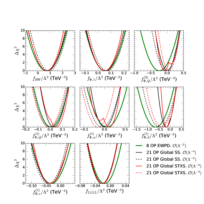
Figure 1: $\Delta\chi^{2}$ as a function of the Wilson coefficients $f_{BW}/\Lambda^{2}$, $f_{\Phi,1}/\Lambda^{2}$, $f^{(1)}_{\Phi,Q}/\Lambda^{2}$, $f^{(3)}_{\Phi,Q}/\Lambda^{2}$, $f^{(1)}_{\Phi,u}/\Lambda^{2}$, $f^{(1)}_{\Phi,d}/\Lambda^{2}$, $f^{(1)}_{\Phi,e}/\Lambda^{2}$, and $f_{LLLL}/\Lambda^{2}$, as indicated in the panels after marginalizing over the remaining fit parameters. The green solid line stands for the fit of the EWPD that constrains only eight of twenty one Wilson coefficients in Eq. (5). The red solid (dashed) line represents the twenty-one-parameter fit to the LHC Run 1 and 2 data including the STXS Higgs data and working at order $1/\Lambda^{4}$ ($1/\Lambda^{2}$) approximation. For comparison, we present the corresponding results for the global fit using the SS Higgs data (black solid and dashed lines).

In the upper left and central panels of Fig. 1, we find the $\Delta\chi^{2}$ dependence on $f_{BW}/\Lambda^{2}$ and $f_{\Phi,1}/\Lambda^{2}$ which correspond to the $S$ and $T$ oblique corrections respectively. For these coefficients, the EWPD limits are only slightly improved just by the global analysis including the STXS Higgs data when the theoretical predictions include the quadratic contributions of the Wilson coefficients.

Turning to the quark gauge couplings, the right upper (left central) panel in Fig. 1 present the $\Delta\chi^{2}$ dependence on the coefficient $f^{(3)}_{\Phi,Q}/\Lambda^{2}$ ($f^{(1)}_{\Phi,Q}/\Lambda^{2}$), which modifies the couplings of left-handed quarks to $Z$ and $W$ (only $Z$) bosons. The middle and right central panels correspond to the dependence on $f^{(1)}_{\Phi,u}/\Lambda^{2}$ and $f^{(1)}_{\Phi,d}/\Lambda^{2}$ which give corrections to the $u_{R}$ and $d_{R}$ couplings to $Z$ respectively. The inclusion of the LHC observables leads to a small but not negligible improvement on the determination of $f^{(1)}_{\Phi,u}/\Lambda^{2}$ at linear order, while it only affects the EWPD bounds on $f^{(1)}_{\Phi,Q}/\Lambda^{2}$ when ${\cal O}(\Lambda^{-4})$ terms are included in the LHC analysis. The largest effect of the combination with the LHC observables occurs for $f^{(3)}_{\Phi d}/\Lambda^{2}$ and $f^{(3)}_{\Phi,Q}/\Lambda^{2}$. In particular the EWPD analysis favors non-vanishing values for $f^{(1)}_{\Phi d}/\Lambda^{2}$ at 2$\sigma$, a result driven by the 2.7$\sigma$ discrepancy between the observed $A_{\rm FB}^{0,b}$ and the SM. On the contrary, the inclusion of the LHC data gives rise to a shift towards zero of $f^{(1)}_{\Phi d}/\Lambda^{2}$, reducing the tension with the SM. This behavior was already observed in Refs. Alves et al. (2018); da Silva Almeida et al. (2019b) but we find now that with the accumulated statistics, LHC also is able to provide relevant constraints when including the effect of dimension-six operators only at ${\cal O}(\Lambda^{-2})$. As the LHC observables included are mostly sensitive to gauge couplings of the light quarks in the parton distribution functions, one expects that this result relies upon the assumption that the operators involving fermion couplings to gauge bosons are generation independent. To test this, we perform an analysis in which we drop this assumption for the operator $f^{(1)}_{\Phi d}/\Lambda^{2}$ and allow $f^{(1)}_{\Phi,d_{11}}=f^{(1)}_{\Phi,d_{22}}\neq f^{(1)}_{\Phi,d_{33}}$ . The results are shown in Fig. 2 where we display the bounds imposed by the EWPD on the relevant quark operators with those from the global STXS analysis including up to ${\cal O}(\Lambda^{-2})$ and up to ${\cal O}(\Lambda^{-4})$ terms. Comparing with the corresponding panels in Fig. 1 we see that the combination of EWPD with the LHC observables results in the quoted improvement on the bounds for those operators contributing to the light quark couplings. Conversely $f^{(1)}_{\Phi,d_{33}}$ is only marginally affected by the inclusion of the EWDBD and Higgs data and its best fit remains no-zero at $\sim 2\,\sigma$ in the global analysis.

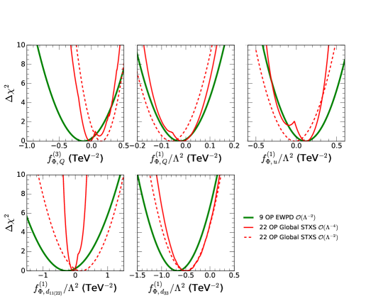
Figure 2: $\Delta\chi^{2}$ as a function of the Wilson coefficients contributing to the gauge couplings of the quarks for non-universal right-handed quark coupling of the bottom quark, this is for $f^{(1)}_{\Phi,d_{1}}=f^{(1)}_{\Phi,d_{2}}\neq f^{(1)}_{\Phi,d_{3}}$. green solid line stands for the fit of the EWPD that constrains only nine of twenty two Wilson coefficients. The red solid (dashed) line represents the twenty-one-parameter fit to the LHC Run 1 and 2 data including the STXS Higgs data and working at order $1/\Lambda^{4}$ ($1/\Lambda^{2}$) approximation.

Finally, the lower panels of Fig. 1 display the marginalized $\Delta\chi^{2}$ for $f^{(1)}_{\Phi,e}/\Lambda^{2}$ and $f_{LLLL}/\Lambda^{2}$. The global analyses do not lead to significant improvement on the determination of these couplings. This is expected since the operator ${\cal O}^{(1)}_{\Phi,e}$ modifies the $Z$ coupling to right-handed leptons which were very precisely tested at LEP. On the contrary, it enters the LHC observables only via its contribution to the decay rate of the $Z$ boson to leptons in some of the final states considered. In other words, the dominant dependence of the global analysis on these coefficients still resides in the EWPD. The main effect of the inclusion of the LHC results is indirect via the restriction of the allowed range of variation of the other coefficients entering in the EWPD analysis.

IV.2 Triple anomalous gauge couplings constraints

We present our results on the Wilson coefficients of the TGC operators ${\cal O}_{B}$, ${\cal O}_{W}$ and ${\cal O}_{WWW}$ in Fig. 3. We first consider the twelve-dimensional parameter space

$$\left\{f_{B},f_{W},f_{WWW},f_{BW},f_{\Phi,1},f^{(3)}_{\Phi,Q},f^{(1)}_{\Phi,Q},f^{(1)}_{\Phi,u},f^{(1)}_{\Phi,d},f^{(1)}_{\Phi,ud},f^{(1)}_{\Phi,e},f_{LLLL}\right\}$$

and include the EWDBD and EWPD. The upper (lower) panels contain the one–dimensional $\Delta\chi^{2}$ distributions after marginalization over the 11 undisplayed coefficients and they were obtained using the up to quadratic (linear) contributions of the 12 Wilson coefficients. Each panel shows as dashed lines the impact of the different diboson data sets and as full black line the combined EWPD+EWDBD analysis. For comparison we also show the corresponding projections obtained from the global STXS fit performed in the the 21 parameter space (red lines).

In what respects $f_{B}/\Lambda^{2}$ we find that EWPD+EWDBD provides only lose constraints on this parameter at ${\cal O}(\Lambda^{-2})$ (see black line in the lower left panel of Fig. 3). Comparing with the black line in the upper left panel of the figure we see how the inclusion of the ${\cal O}(\Lambda^{-4})$ terms leads to better bounds, with the $WW$ channel (blue dashed line) playing the dominant role. This is so even though the integrated luminosity is larger for the $W\gamma$ data than for $WW$, because the $W\gamma$ data depends on the combination $(f_{B}/\Lambda^{2}+f_{W}/\Lambda^{2})$ which allows for cancellations between $f_{B}/\Lambda^{2}$ and $f_{W}/\Lambda^{2}$. Similarly the $WZ$ channel also depends on $f_{B}/\Lambda^{2}$ in another linear combination with $f_{W}/\Lambda^{2}$ and furthermore its coefficient is suppressed by a factor $\tan^{2}\theta_{W}$ with respect to the $f_{W}/\Lambda^{2}$. From these panels we also conclude that $f_{B}/\Lambda^{2}$ is much more strongly constrained by the global analysis (red lines) than by the EWPD+EWDBD. This is so because ${\cal O}_{B}$ contributes to both Higgs production and decay. This fact was observed before in Ref. Corbett et al. (2013b). But we find now that with the large Run 2 luminosity and the STXS information, the constraints on $f_{B}/\Lambda^{2}$ are substantially improved even when including the dimension-six parameters only up to ${\cal O}(\Lambda^{-2})$.

The $\Delta\chi^{2}$ distributions for $f_{W}/\Lambda^{2}$ are displayed in the middle panels where we see that the dominant diboson channels constraining $f_{W}/\Lambda^{2}$ are the $WW$ and $WZ$. Here too, $W\gamma$ production is not able to produce any sensible bound on $f_{W}/\Lambda^{2}$ due to its (anti-)correlation with $f_{B}/\Lambda^{2}$ previously commented. In this case the limits obtained at ${\cal O}(\Lambda^{-2})$ are already rather stringent and they are significantly improved by the global analysis.

In order to show the importance of the Higgs data in constraining $f_{B}/\Lambda^{2}$ and $f_{W}/\Lambda^{2}$ we present in Fig. 4 the $1\sigma$ and $2\sigma$ allowed regions of the plane $f_{B}/\Lambda^{2}\times f_{W}/\Lambda^{2}$ obtained with different data samples. These results were obtained using only the contributions up to ${\cal O}(\Lambda^{-2})$ on the Wilson coefficients and the SS (STXS) Higgs data on the left (right) panel. As we can see the EWPD+EWDBD data sets lead to a very large allowed region (pink regions). The constraints coming from the SS Higgs data (shown in the green regions on the left panel in combination with the EWPD ) are also loose but they are important to improve the limits when combined also with the EWDBD. But most interestingly, as seen in the right panel, using only the Higgs STXS analysis in combination with EWPD (right panel), is able to place much stronger bounds on $f_{W}/\Lambda^{2}$ and $f_{B}/\Lambda^{2}$ ; compare the green and pink regions. Clearly, the global fit on ${\cal O}_{B}$ is dominated by the data samples in the Higgs STXS analysis while the constraints on ${\cal O}_{W}$ receives comparable contributions from Higgs STXS and EWDBD.

At last, the right panels of Fig. 3 contain the dependence of the marginalized $\Delta\chi^{2}$ on $f_{WWW}/\Lambda^{2}$. In contrast to $f_{B}/\Lambda^{2}$ and $f_{W}/\Lambda^{2}$, the channel $W\gamma$ plays a significant role in constraining $f_{WWW}/\Lambda^{2}$ due to the use of kinematic distributions specially chosen to avoid the cancellation of the $1/\Lambda^{2}$ contribution  Azatov et al. (2017, 2019). In fact, we can see from the lower right panel of this figure that the most important contributions to the EWPD+EWDBD analysis originates from those channels ($W\gamma$ and $Zjj$). Also, as expected, the global analysis has barely any additional impact on limiting ${\cal O}_{WWW}$ since this operator does not contribute to the Higgs observables.

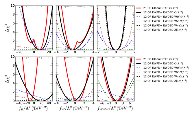
Figure 3: $\Delta\chi^{2}$ dependence on the $f_{B}/\Lambda^{2}$ (left panels), $f_{W}/\Lambda^{2}$ (central panels) and $f_{WWW}/\Lambda^{2}$ (right panels) parameters after the marginalization over the 11 (20) undisplayed fit parameters for the analysis of EWDBD+EWPD (global STXS) data as labeled in the figure. The upper panels show the results of our analysis using up to ${\cal O}(\Lambda^{-4})$ terms in the Wilson coefficients while the lower ones retained only the ${\cal O}(\Lambda^{-2})$ terms.

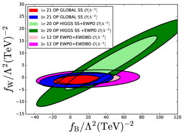
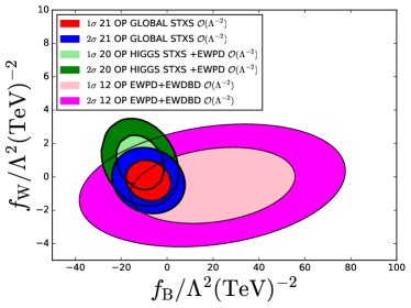
Figure 4: $1\sigma$ and $2\sigma$ (2dof) allowed regions on the $f_{B}/\Lambda^{2}\times f_{W}/\Lambda^{2}$ plane obtained from the analysis of different combinations of data samples as labeled in the figure. All results use predictions up to the ${\cal O}(\Lambda^{-2})$ terms in the Wilson coefficients and have been marginalized over the undisplayed ones.

IV.3 Higgs couplings

In order to probe for deviations from the SM predictions to the Higgs couplings we performed four global fits including the effects of the 21 operators in Eqs. (2)–(4) under different assumptions. As mentioned in Sec. III in order to access the importance of the newly available kinematic distributions we made two analysis: one in which that information is not included (Global SS) and another one in which it is (Global STXS). And, as for EWDBD, we make two variants of the analysis, one employing the theoretical predictions up to ${\cal O}(\Lambda^{-2})$ terms in the Wilson coefficients, and one including up to ${\cal O}(\Lambda^{-4})$ terms.

We have discussed in the context of Figs. 1 and 3 the results from these global analysis for the 12 operators that contribute also to the EWPD and EWDBD, therefore, we focus here on the nine operators not studied yet. We show in Fig. 5 the dependence of the marginalized $\Delta\chi^{2}_{\rm global}$ on each of these nine Wilson coefficients for the four analysis variants.

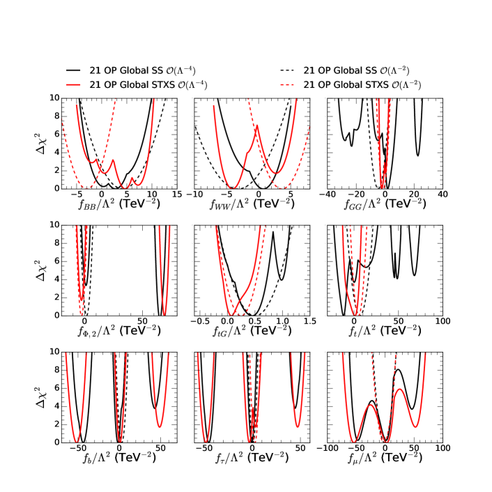
Figure 5: Marginalized $\Delta\chi^{2}$ distributions as a function of the Wilson coefficients for the nine operators that only affect the Higgs physics and for the four variants of the global analysis as labeled in the figure (see text for details).

From Fig. 5 we observe , as expected, that for the analysis including only the contributions up to ${\cal O}(\Lambda^{-2})$ (dashed lines) there is a unique minimum in either the global SS or global STXS analysis. And comparing the red and black dashed lines we conclude that at ${\cal O}(\Lambda^{-2})$ the impact of the STXS observables in the overall picture amounts to an uncertainty reduction of 30–40% for some of the bosonic operators as well as a shift in the allowed region in a few cases.

Conversely, we also see in Fig. 5 that for the analysis including up to ${\cal O}(\Lambda^{-4})$ terms and the SS samples for the Higgs data (solid black lines) all panels present some set of (quasi)degenerated minima. They are a direct reflect of the (quasi)degeneracies in the Higgs couplings in Eqs. (6)–(9). Comparing the solid black and red lines we see the relevance of the kinematic distributions in resolving some of these degeneracies.

First, let us focus on the left central panel of Fig. 5 which depicts the $\Delta\chi^{2}$ distribution as a function of $f_{\Phi,2}/\Lambda^{2}$. In the SS analysis at ${\cal O}(\Lambda^{-4})$, there are two clearly almost degenerate minima associated with the flip of sign of all Higgs couplings discussed below Eq. (6) for $f_{\Phi,2}/\Lambda^{2}\simeq 65$ TeV^-2. In fact we find that the analysis show a slight preference for this non-standard solution. As seen in the figure, this is still the case once the information of the STXS observables is included but the $\Delta\chi^{2}$ of the SM-connected solution is reduced to $\sim 1.3\;\sigma$.

The power of the kinematic distributions is particularly striking for the coefficients $f_{GG}/\Lambda^{2}$ , $f_{t}/\Lambda^{2}$ and $f_{tG}/\Lambda^{2}$ which, together with $f_{\Phi,2}/\Lambda^{2}$, enter in the effective gluon-gluon Higgs vertex and for which the marginalized $\chi^{2}$ for the global SS analysis shown in the black curves in Fig. 5 present a complex structure of local minima. This is further illustrated in Fig. 6. In this figure we show the allowed regions from the global analysis performed at ${\cal O}(\Lambda^{-4})$, projected over pairs of these parameters (after marginalization over the 19 undisplayed parameters in each panel). We observe the complex structure of allowed regions in $f_{GG}/\Lambda^{2}\times f_{\Phi,2}/\Lambda^{2}$, $f_{GG}/\Lambda^{2}\times f_{t}/\Lambda^{2}$ and $f_{tG}/\Lambda^{2}\times f_{\Phi,2}/\Lambda^{2}$ that appear in the SS ${\cal O}(\Lambda^{-4})$ analysis . As inferred from the figure, the inclusion of the Higgs kinematic distributions in the analysis is able to fully separate the contribution from ${\cal O}_{GG}$, ${\cal O}_{tG}$, and ${\cal O}_{u\Phi,33}$ while the degeneracy associated to ${\cal O}_{\Phi,2}$ remains.

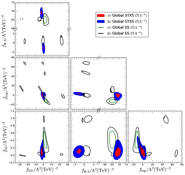
Figure 6: $1\sigma$ and 95% CL (2dof) allowed regions from the SS and STXS global analysis for the coefficients of the operators entering in the gluon-gluon Higgs vertex (Eq. (9)). These results were obtained using terms up to ${\cal O}(\Lambda^{-4})$ of the theoretical prediction, and the color code indicates the used data set as labeled in the figure.

We now turn to the operators involved in the photon-photon-Higgs vertex. The upper left and central panels of Fig. 5 contain $\Delta\chi^{2}$ as a function of $f_{BB}/\Lambda^{2}$ and $f_{WW}/\Lambda^{2}$ respectively. The four analyses, SS and STXS with predictions at ${\cal O}(\Lambda^{-2})$ and ${\cal O}(\Lambda^{-4})$, lead to a unique allowed range for both Wilson couplings compatible with the SM at $2\sigma$ level but for the STXS analysis at ${\cal O}(\Lambda^{-4})$ we still observe several minima. To better understand these results we present in Fig. 7 $1\sigma$ and 95% CL (2dof) allowed regions from the SS and STXS global analyses in the plane $f_{BB}/\Lambda^{2}\times f_{WW}/\Lambda^{2}$. From the figures we see that all allowed regions display the strong anti-correlation between those parameters associated with the $(f_{WW}+f_{BB})/\Lambda^{2}$ dependence of the Higgs-photon-photon vertex. This correlation is not exact because it is broken by other measurements, in particular by the $HF_{\mu\nu}Z^{\mu\nu}$ branching ratio which constrains a different combination $f_{WW}/\Lambda^{2}$ and $f_{BB}/\Lambda^{2}$. In the figure we also observe the existence of the second allowed region(s) around $(f_{WW}+f_{BB})/\Lambda^{2}\sim 3$ TeV^-2 in the analysis performed to ${\cal O}(\Lambda^{-4})$, associated to the flip of sign of the Higgs-photon-photon coupling with respect to the SM value discussed below Eq.(8). In this case, unlike for the gluon-gluon-Higgs vertex, the kinematic information contained in the STXS observables cannot resolve these two solutions for which the kinematics is identical. In addition there are two solutions for each of those mirror solutions associated to the degeneracy associated with $f_{\Phi,2}$ which affects the production cross section. For the STXS analysis the two solutions become separated enough to lead to the two additional disconnected regions observed in the right panel. Further details can be obtained from the correlation matrices presented in appendix A.

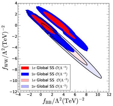
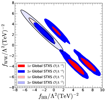
Figure 7: $1\sigma$ and 95% CL (2dof) allowed regions from the (STXS) SS global analysis in the plane $f_{BB}/\Lambda^{2}\times f_{WW}/\Lambda^{2}$ on the left (right) panel. These results were obtained using the theoretical predictions up to ${\cal O}(\Lambda^{-2})$ or up to ${\cal O}(\Lambda^{-4})$ approximations, as indicated by the color code.

In what respects the Yukawa couplings $Hff$, as discussed in Sec. II, they exhibit a four-folded degeneracy in the ${\cal O}(\Lambda^{-4})$ analysis because the sign of this coupling can be flip by $f_{\Phi,2}/\Lambda^{2}$ and $f_{f}/\Lambda^{2}$; see Eq. (7). This degeneracy favors the existence of three disconnected allowed ranges da Silva Almeida et al. (2019b) and it is clearly observable in both analyses at ${\cal O}(\Lambda^{-4})$ in the three lower panels in Fig. 5 for the bottom, $\tau$ and $\mu$ Yukawas as well as in the left panel of Fig. 8. These solutions are not totally degenerate because, as discussed above, in the ${\cal O}(\Lambda^{-4})$ analysis we find a slight preference for the non-standard solution for $f_{\Phi,2}/\Lambda^{2}$. Including the kinematic information in the form of the STXS observables does not resolve this degeneracy.

For $f_{t}/\Lambda^{2}$ the four-folded degeneracy is expect to be partially broken since the scattering amplitude for the $tH$ production receives contributions from the $ttH$ and $VVH$ vertices, therefore, being sensitive to the relative sign of the different diagrams contributing  Barger et al. (2010); Biswas et al. (2013); Chang et al. (2014). Conversely, the contribution of this coupling to the effective gluon-gluon-Higgs vertex introduces the additional degeneracy/correlations with $f_{GG}$ and $f_{tG}$ described above. Altogether, we find that the STXS Higgs data is able to constrain univocally the top Yukawa coupling even at ${\cal O}(\Lambda^{-4})$.

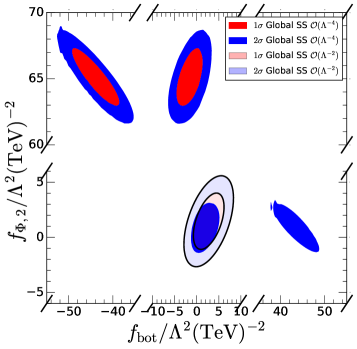
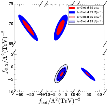
Figure 8: $1\sigma$ and 95% CL (2dof) allowed regions from the STXS global analysis in the plane $f_{\Phi,2}/\Lambda^{2}\times f_{b}/\Lambda^{2}$. These results were obtained using the Higgs SS and STXS data keeping the quadratic terms of the theoretical prediction, as indicated by the color code.

We present the one sigma bounds and correlations in appendix A for the ${\cal O}(\Lambda^{-2})$ global SS and STXS analysis. From these results we can see that the strongest (anti-)correlations are between the pairs of operators ${\cal O}_{B}\otimes{\cal O}_{BB}$, ${\cal O}_{B}\otimes{\cal O}_{WW}$, ${\cal O}_{BB}\otimes{\cal O}_{WW}$, ${\cal O}_{GG}\otimes{\cal O}_{u\Phi,33}$, ${\cal O}_{GG}\otimes{\cal O}_{tG}$, ${\cal O}_{BW}\otimes{\cal O}_{\Phi,1}$, and ${\cal O}^{(1)}_{\Phi,e}\otimes{\cal O}_{LLLL}$. The first three stems mainly from the Higgs decay into photon pairs, while the next two are due to the Higgs coupling to gluons, and the last two are dominantly due to their contribution to the EWPD observables. Furthermore, ${\cal O}_{\Phi,2}$ possesses sizable correlations with many dimension-six operators due to the possibility of flipping the sign of the Higgs couplings.

V Results for Simplified Models

Figures 9 and  10 contain the results of the analyses for the simplified models presented in Sec. II.1.

The $\Delta\chi^{2}$ distribution for the singlet scalar extension of the SM is presented in the left panel of Fig. 9, for both global analysis and the predictions obtained up to ${\cal O}(\Lambda^{-2})$ and up to ${\cal O}(\Lambda^{-4})$, which lead to similar results. We find, for example, that considering only the effects at order ${\cal O}(\Lambda^{-2})$ the bound obtain from the SS analysis is

$$|\sin\theta|<0.279\;\;$$ (19)

at 95% CL. This model only generates $f_{\Phi,2}/\Lambda^{2}$ at tree level, therefore, we can translate the above limit into $f_{\Phi,2}/\Lambda^{2}<1.4$ TeV^-2 using Eq. (10). Notice that this constraint is about 4 times stronger than the than the limit originating from the 21-parameter analysis; see Table 6. Also, this limit is similar to that that derived in Ref. Atlas Collaboration (2020).

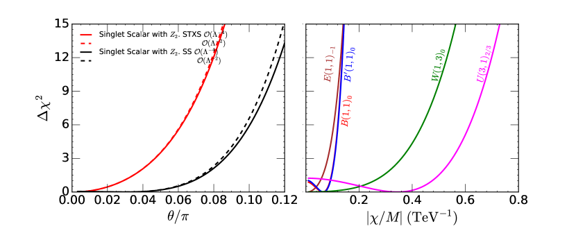
Figure 9: The left (right) panel contains $\Delta\chi^{2}$ as a function of $\theta/\pi$ ($\chi/M$) for the singlet scalar model (models with one additional state). The results shown on the right panel correspond to the global analysis with the STXS Higgs data sets and including only the contributions that are linear on the Wilson coefficients (${\cal O}(\Lambda^{-2})$).

The $\Delta\chi^{2}$ distributions for the simplified models that contain the addition of one state described in Table 3 can be found in the right panel of Fig. 9. For concreteness, we show the results for the global STXS analysis at ${\cal O}(\Lambda^{-2})$, but for these models the inclusion of the quadratic terms has a very little impact indicating the stability of the results with respect to higher orders corrections as well as the validity of the high mass expansion. From the figure we read the following 95% CL bounds on $\chi^{2}/M$, which implies the quoted mass limit for $\chi=1$:

$$\frac{\chi}{M}<0.084\;{\rm TeV}^{-1} \;\;\;(M>12\;{\rm TeV})\;\;\; {\rm Model\;with\;}E(1,1)_{-1}\;\;,$$

$$\frac{\chi}{M}<0.15\;{\rm TeV}^{-1} \;\;\;(M>6.7\;{\rm TeV})\;\;\; {\rm Model\;with\;}B^{\prime}(1,1)_{0}\;\;,$$

$$\frac{\chi}{M}<0.16\;{\rm TeV}^{-1} \;\;\;(M>6.2\;{\rm TeV})\;\;\; {\rm Model\;with\;}B(1,1)_{-1}\;\;,$$ (20)

$$\frac{\chi}{M}<0.35\;{\rm TeV}^{-1} \;\;\;(M>2.8\;{\rm TeV})\;\;\; {\rm Model\;with\;}W(1,3)_{0}\;\;,$$

$$\frac{\chi}{M}<0.58\;{\rm TeV}^{-1} \;\;\;(M>1.7\;{\rm TeV})\;\;\; {\rm Model\;with\;}U(3,1)_{2/3}\;\;.$$

The tightest constraint is for the model containing a new lepton $E$ (brown curve) since this model generates the strongly bound Wilson coefficients $f^{(1)}_{\Phi,e}/\Lambda^{2}$ and $f_{\Phi,1}/\Lambda^{2}$, which appear when the Wilson coefficients generated at the high scale matching are rotated to the HISZ basis using Eqs. (12) and (13). The models with an extra vector $B$ are also subject to strong limits because they generate $f_{\Phi,1}/\Lambda^{2}$ i.e. they contribute to the $T$ parameter.

The additional vector triplet $W$ and the extra vector quark $U$ prompts the appearance of the Wilson coefficient $f^{(3)}_{\Phi,Q}/\Lambda^{2}$ which is well constrained by the precise determination of the electroweak gauge couplings of left-handed quarks with EWPD and LHC diboson Alves et al. (2018) and Higgs associated production Biekoetter et al. (2019); Brehmer et al. (2019) data. The extra vector quark $U$ generates also $f^{(1)}_{\Phi,Q}/\Lambda^{2}$ but with opposite sign. $f^{(1)}_{\Phi,Q}/\Lambda^{2}$ also contributes to the couplings of the left-handed quarks to the $Z$ boson, what leads to a small anti-correlation between these two coefficients. This results into the slighter weaker bounds in this model.

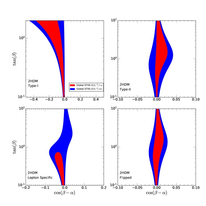
Figure 10: Allowed regions of the plane $\cos(\beta-\alpha)\times\tan\beta$ for several two Higgs doublet models. The results shown correspond to the global analyses with the STXS Higgs data sets including only the contributions that are linear on the Wilson coefficients (${\cal O}(1/\Lambda^{2})$).

Figure 10 contains the constraints on 2HDMs that we obtain performing the global analysis at ${\cal O}(\Lambda^{-2})$ and using the STXS Higgs data sets. In the figure, we see that the allowed range for $\cos(\beta-\alpha)$ is tightly constrained in agreement with the alignment assumption with the only exception of the Type-I model in the large $\tan\beta$ limit for which the Wilson coefficients we are considering approach zero and, therefore, no bound can be imposed in this approximation. In fact, with that exception our results show that the allowed parameter space at 95% CL is strongly bounded. Compared to the experimental results obtained in Ref. Sirunyan et al. (2019b) that used just a fraction of the Run 2 integrated luminosity we find stronger bounds on $\cos(\beta-\alpha)$, for fixed $\tan\beta$ by up to a factor 4 depending on the model and the sign of $\cos(\beta-\alpha)$. Also in our analysis we do not find the small lobe features observed in Ref. Sirunyan et al. (2019b) for positive $\cos(\beta-\alpha)$ and large $\tan\beta$. Our bounds on Type-I and II models are comparable with those derived in Ref. Dawson et al. (2020); Khosa and Sanz (2021).

VI Discussion

In this work we have presented the results of comprehensive analyses of low-energy electroweak precision measurements as well as LHC data on gauge boson pair production and Higgs observables in the context of the SMEFT. We focused on observables related to the electroweak sector, which at present allow for precision tests of the couplings between electroweak gauge bosons and fermions, triple electroweak gauge couplings and the couplings of the Higgs to fermions and gauge bosons. For the sake of assessing the impact of the Higgs kinematic distributions we performed an analysis with and without the STXS Higgs data in combination with the Higgs total signal strengths. In total, the global analyses of EWPD and EWDBD and Higgs results from LHC encompasses 167 observables when considering only SS data and 255 observables when including the STXS samples; see Sec. III for further details.

We worked in the framework of effective lagrangians assuming the linear realization of the electroweak gauge symmetry. Dimension-six operators are those with lowest dimension which contribute significantly to the considered processes at lowest order. The global analysis involves the 21 operators in Eq. (5) under the flavor assumption that the new operators do not introduce additional tree level sources of flavor violation nor violation of universality of the weak current. Furthermore, we also analyzed the constraints on a few simplified models to illustrate how relations between the generated Wilson coefficients within specific models lead to tighter limits.

All of the analyses performed show no statistically significant source of tension with the SM. We find

$$\chi^{2}_{\rm min\;EWPD+EWDBD,\;SM}=91\;, {\rm\;111\;observables\;,}$$

$$\chi^{2}_{\rm min\;Global\ SS,\;SM}=133\;, {\rm\;166\;observables\;,}$$ (21)

$$\chi^{2}_{\rm min\;Global\ STXS,\;SM}=304\;, {\rm 255\;observables\;},$$

to be compared with

$$\chi^{2}_{\rm min\;EWPD+EWDBD,\;SMEFT\,{\cal O}(\Lambda^{-4})\;[SMEFT\,{\cal O}(\Lambda^{-2})]}=87\;[85], {\rm\;111\;observables\;\&\;12\;operators\;,}$$

$$\chi^{2}_{\rm min\;Global\ SS,SMEFT\,{\cal O}(\Lambda^{-4})\;[SMEFT\,{\cal O}(\Lambda^{-2})]}=115\;[112], {\rm\;166\;observables\;\&\;21\;operators\;,}$$ (22)

$$\chi^{2}_{\rm min\;Global\ STXS,\;SMEFT\,{\cal O}(\Lambda^{-4})\;[SMEFT\,{\cal O}(\Lambda^{-2})]}=266\;[264], {\rm 255\;observables\;\&\;21\;operators\;}.$$

We summarize our results of the $\chi^{2}$ dependence on the Wilson coefficients for the ${\cal O}(\Lambda^{-2})$ and ${\cal O}(\Lambda^{-4})$ analyses, which we performed with the most comprehensive data set including the kinematic information on the Higgs observables, by displaying the corresponding one-dimensional $\Delta\chi^{2}$ distributions shown in Fig. 11, where we marginalized over the 20 undisplayed variables in each panel. With these results and the corresponding ones for the global SS analysis we obtain the 95% CL allowed ranges of the 21 Wilson coefficients that we present in Table 6 and graphically display them in Fig. 12. The maximum allowed value for each Wilson coefficient at a given CL can be translated into a lower bound bound on an effective new physics scale

$$\Lambda_{\rm min,CL}\equiv\frac{1}{\sqrt{|f/\Lambda^{2}|_{\rm max,CL}}}\;\;,$$ (23)

that are depicted in Fig. 13. Notice that $\Lambda_{\rm min,CL}$ only coincides with the minimum energy scale in the operator expansion, $\Lambda$, for coefficients $f=1$. $\Lambda$ could be smaller than $\Lambda_{\rm min,CL}$ if the coupling is weak.

Operator	95% CL $f/\Lambda^{2}$ (TeV-2)
	Global SS ${\cal O}(\Lambda^{-4})$,	Global SS ${\cal O}(\Lambda^{-2})$,	Global STXS ${\cal O}(\Lambda^{-4})$,	Global STXS ${\cal O}(\Lambda^{-2})$,
${\cal O}_{B}$	(-9.8,14)	(-5.5,37)	(-11,15)	(-23,3.0)
${\cal O}_{W}$	(-2.0,2.8)	(-3.0,2.6)	(-2.0,2.7)	(-1.2,2.3)
${\cal O}_{WWW}$	(-0.80,0.81)	(-3.5,4.5)	(-0.81,0.78)	(-4.1,4.2)
${\cal O}_{BB}$	(-2.8,7,5)	(-1.2,9.6)	(-3.4,9.4)	(-6.6,0.65)
${\cal O}_{WW}$	(-3.9,3.7)	(-8.3,1.8)	(-6.1,-1.7) $\,\cup\,$ (0.78,4.5)	(0.30,7.9)
${\cal O}_{GG}$	(-1.0,5.7) $\,\cup\,$ (22,23)	(-9.7,0.23)	(-3.7,1.4)	(-4.3,1.7)
${\cal O}_{tG}$	(0.11,0.71)	(0.073,0.93)	(-0.010,0.48)	(-0.035,-0.53)
${\cal O}_{\Phi,2}$	(0.33,2.0)$\,\cup\,$(62,68)	(-1.7,5.2)	(-4.7,-0.71)$\,\cup\,$(66,72)	(-5.7,0.26)
${\cal O}_{u\Phi,33}$	(-18,-7,3)$\,\cup\,$(-1.3,1.7)	(-2.8,16)	(-10,5.9)	(-0.89,11)
${\cal O}_{d\Phi,33}$	(-52,-37)$\,\cup\,$(-5.6,3.3) $\,\cup\,$ (41,45)	(-1.6,7.8)	(-60,-44)$\,\cup\,$(-3.5,5.2)$\,\cup\,$ (44,54)	(-2.8,5.0)
${\cal O}_{e\Phi,33}$	(-50,-40)$\,\cup\,$(-3.7,2.7) $\,\cup\,$(44,45)	(-2.5,4.2)	(-53,-43)$\,\cup\,$(-7.0,6.2) $\,\cup\,$(43,51)	(-0.64,6.3)
${\cal O}_{e\Phi,22}$	(-57,-28)$\,\cup\,$(-18,11) $\,\cup\,$(41,51)	(-14,12)	(-69,-30)$\,\cup\,$(-22,15) $\,\cup\,$(39,62)	(-15,11)
${\cal O}_{BW}$	(-0.21,1.7)	(-0.064,1.8)	(-0.19,1.6)	(-0.22,1.7)
${\cal O}_{\Phi,1}$	(-0.040,0.14)	(-0.024,0.16)	(-0.037,0.14)	(-0.037,0.14)
${\cal O}^{(3)}_{\Phi,Q}$	(-0.23,0.23)	(-0.30,0.24)	(-0.25,0.26)	(-0.15,0.27)
${\cal O}^{(1)}_{\Phi,Q}$	(-0.041,0.10)	(-0.091,0.085)	(-0.034,0.11)	(-0.098,0.075)
${\cal O}^{(1)}_{\Phi,u}$	(-0.22,0.24)	(-0.34,0.22)	(-0.26,0.29)	(-0.41,0.094)
${\cal O}^{(1)}_{\Phi,d}$	(-0.42,0.10)	(-0.95,0.0096)	(-0.34,0.11)	(-0.81,-0.054)
${\cal O}^{(1)}_{\Phi,ud}$	(-0.13,0.13)	—	(-0.12,0.12)	—
${\cal O}^{(1)}_{\Phi,e}$	(-0.076,0.0040)	(-0.081,-0.0016)	(-0.072,0.0020)	(-0.074,-0.0040)
${\cal O}_{LLLL}$	(-0.046,0.0035)	(-0.047,0.0029)	(-0.045,0.0046)	(-0.046,0.0034)

Table 6: Marginalized 95% CL allowed ranges for the Wilson coefficients for the four different global analyses performed in this work.

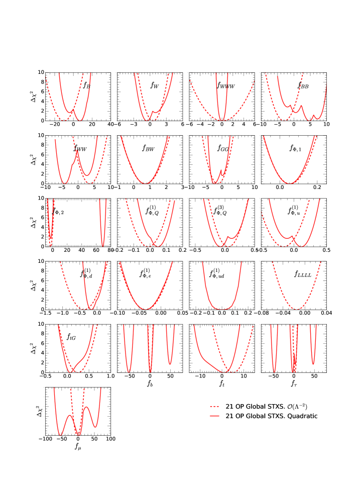
Figure 11: Marginalized one-dimensional $\Delta\chi^{2}$ distributions for the 21 parameters appearing in our global fit including the STXS Higgs data sets. The dashed (solid) line stands for the results obtained with the theoretical predictions for the observables expanded at ${\cal O}(\Lambda^{-2})$ ( ${\cal O}(\Lambda^{-4})$) in the Wilson coefficients.

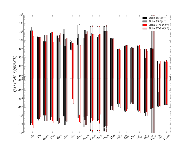
Figure 12: 95% CL on the 21 Wilson coefficients used in our analyses. The color code indicates the data set used and the order of the predictions used.

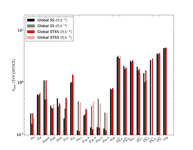
Figure 13: 95% CL minimal effective scale for each of the 21 Wilson coefficients. The color code indicates the data set used and the order of the predictions used.

In brief, the main results that we would like to stress are:

• In our basis there is no blind direction in the electroweak precision observables. Therefore, the limits originating from EWPD are already stringent on eight Wilson coefficients. In fact, the EWPD dominates the bounds on ${\cal O}_{LLLL}$, ${\cal O}^{(1)}_{\Phi,e}$, ${\cal O}_{\Phi,1}$, ${\cal O}_{BW}$, and $f^{(1)}_{\Phi,Q}/\Lambda^{2}$ up to some small but not negligible contribution from LHC data (see Fig. 1).

• Conversely, the global analysis results into a sizable reduction of the uncertainty on $f^{(3)}_{\Phi,Q}/\Lambda^{2}$ with respect to the limits obtained using only EWPD. This is expected due to the role played by this operator in the Higgs associated production Biekoetter et al. (2019); Brehmer et al. (2019).

• The analysis of the EWPD of $f^{(1)}_{\Phi d}/\Lambda^{2}$, points towards a nonzero value for this coefficient due to the 2.7$\sigma$ discrepancy between the observed $A_{\rm FB}^{0,b}$ and the SM. Under the assumption that the operators modifying the fermion-gauge couplings are generation independent, the inclusion of the EWDBD and the Higgs data in the analysis (either SS or STXS) gives rise to a result compatible with the SM at better than 95% CL and with slightly reduced errors. In addition, the global constraint on $f^{(1)}_{\Phi u}/\Lambda^{2}$ is also slightly improved by combining EWPD with the LHC results.

• Allowing for $f^{(1)}_{\Phi d}/\Lambda^{2}$ to be different for the bottom quark, the combination of EWPD with the LHC observables results in the quoted improvement on the bounds for those operators contributing to the light quark couplings but $f^{(1)}_{\Phi,d_{33}}$ is only marginally affected by the inclusion of the EWDBD and Higgs data and its best fit remains nonzero at $\sim 2\,\sigma$ in the global analysis.

• The operator ${\cal O}^{(1)}_{\Phi,ud}$ induces right-handed charged current couplings for quarks and it can only be bound via its quadratic (${\cal O}(\Lambda^{-4})$) contributions. Including those in the LHC observables its Wilson coefficient can be bounded with precision comparable to that of the other operators affecting gauge-quark couplings; see Fig. 11.

• The new EWDBD lead to a significantly improved sensitivity to ${\cal O}_{WWW}$ that is the only TGC operator that does not contribute to the Higgs couplings. Furthermore, the constraints on $f_{B}/\Lambda^{2}$ and $f_{W}/\Lambda^{2}$ are also significantly tightened, specially when combining the information from both EWDBD and Higgs data, in particular the STXS kinematic distributions; see Figs. 3 and 4.

• As anticipated, the recently available kinematic distributions of the Higgs lead not only to more stringent limits but also remove some the correlations between the different operators entering in the gluon-gluon-Higgs interactions; see Fig. 6.

• Degeneracies associated with the flip of the sign of some Higgs couplings to gauge-bosons and Yukawa couplings, that originate from ${\cal O}_{\Phi,2}$, are not resolved in the present STXS analysis if performed at ${\cal O}(\Lambda^{-4})$. In fact, we can see clearly the effect of the existence of two $f_{\Phi,2}/\Lambda^{2}$ local minima in many panels of Fig. 11.

• One can check the stability of the results of the overall picture by comparing the bounds derived using just the $1/\Lambda^{2}$ contribution with those derived with predictions containing terms up to $1/\Lambda^{4}$; see Fig. 11. From the figure we read that the analysis performed at ${\cal O}(1/\Lambda^{2})$ does not allow for the degenerate solutions associated with the flip of the sign of the Higgs couplings nor the strong correlations induced in the effective gluon-gluon-Higgs interaction or photon-photon-Higgs interaction. Generically, the bounds derived including $1/\Lambda^{4}$ terms are somewhat stronger. This is particularly the case for the coefficients of ${\cal O}_{WWW}$ and ${\cal O}^{(1)}_{\Phi d}$, which dominantly contribute to EWDBD. This stability suggests that the power series on $1/\Lambda$ is under control for the range of energy probed at the LHC Run 2. Notwithstanding, it is also important to notice that diboson production has serious theoretical problems at ${\cal O}(\Lambda^{-2})$ since its differential cross section is negative in some regions of the parameters space Baglio et al. (2017) and the ${\cal O}(\Lambda^{-4})$ terms should be kept in that case.

• As it is well-known, EFTs have limited range of validity which can be signaled, for instance, by the rapid growth of the cross section with the energy and consequent violation of unitarity Corbett et al. (2017); Corbett et al. (2015a). Consequently, it is a matter of concern whether the bounds on the Wilson coefficients, are driven by regions of the phase space where the EFT expansion is no longer valid. Unfortunately, there is no systematic way to truncate the phase space in the observables included in the analysis to avoid such problematic regions. Alternatively, the comparison of the limits obtained by the analyses performed at order $1/\Lambda^{2}$ and $1/\Lambda^{4}$, allows us to estimate the size of the higher order contributions which would be most relevant in those phase-space regions. Our results of this comparison indicate that for most operators the ${\cal O}$($1/\Lambda^{4}$) contribution is smaller than the leading one, indicating that, generically, the analysis uses EFT in its validity range.

• Contrasting with the results of our previous analysis, Ref. Corbett et al. (2015b); Butter et al. (2016); Alves et al. (2018), we find that the bounds on bosonic operators modifying the Higgs couplings are much more stringent once the full LHC Run 2 data is considered. In particular, the kinematic distributions provided in the STXS format allows the derivation of constraints which are a factor 2 to 10 stronger for the Wilson coefficients of ${\cal O}_{B}$, ${\cal O}_{W}$, ${\cal O}_{BB}$, ${\cal O}_{W}$, and ${\cal O}_{GG}$ at at order $1/\Lambda^{2}$.

• At ${\cal O}(\Lambda^{-2})$ the precision on the Yukawa couplings $f_{t}/\Lambda^{2}$, $f_{b}/\Lambda^{2}$, $f_{\tau}/\Lambda^{2}$, and $f_{\mu}/\Lambda^{2}$ are similar using the SS or STXS data sets and their allowed range is reduced by $\sim 30\%$ for $f_{b}$ and $f_{\tau}$, and $\sim 2$ for $f_{\mu}$ with respect to our previous results Alves et al. (2018).

• Despite the added complexity to the higgs-gluon-gluon vertex (see Eq. (9) and Fig. 6), the introduction of the additional contribution (${\cal O}_{tG}$) to the Higgs production via gluon fusion does not affect significantly the analysis once the independent constraint from top physics (Eq. (17)) is included. In addition, the Higgs data set is able to improve slightly the limits on this coefficient, favoring a value closer to zero, with respect to the top physics bias.

• Finally, the study of simplified models shows that the available data sets are able to put stringent limits on the models parameters as we see in Figs. 9 and  10 and Eq. 19 and  20. In particular, for all 2HMD’s variants our analysis results into bounds on $\cos(\beta-\alpha)$, for a fixed $\beta$, which are up to a factor $\sim$ 4 stronger than those derived in the experimental analysis of Ref. Sirunyan et al. (2019b).

Altogether we find that the increased integrated luminosity gathered at 13 TeV allows us to obtain more stringent bounds on a larger set of anomalous interactions and to perform new tests of the SM. So far there is no indication of deviations from the SM predictions.

Appendix A Analytical expresion of $\chi^{2}$ for ${\cal O}(\Lambda^{-2})$ SS and STXS analysis

By definition when the theoretical predictions for the observables considered in the analysis are expanded to linear order (i.e. ${\cal O}(\Lambda^{-2})$) in the Wilson coefficients, $\Delta\chi^{2}$ takes the form

$$\Delta\chi^{2}=\sum_{i=1}^{N}\left(\frac{f_{i}}{\Lambda^{2}}-\frac{f^{0}_{i}}{\Lambda^{2}}\right)\,V^{-1}_{ij}\left(\frac{f_{j}}{\Lambda^{2}}-\frac{f^{0}_{j}}{\Lambda^{2}}\right)\;,$$

where $V$ is the covariance matrix

$$V_{ij}\equiv\sigma_{i}\,\sigma_{j}\,\rho_{ij}\;.$$

For the SS analysis we find the best fit values and uncertainties

$\begin{array}[]{|c|cccccccccccccccccccc|}\hline\cr&{\cal O}_{B}&{\cal O}_{W}&{\cal O}_{WWW}&{\cal O}_{BB}&{\cal O}_{WW}&{\cal O}_{GG}&{\cal O}_{tG}&{\cal O}_{\Phi,2}&{\cal O}_{u\Phi,33}&{\cal O}_{d\Phi,33}&{\cal O}_{e\Phi,33}&{\cal O}_{e\Phi,22}&{\cal O}_{BW}&{\cal O}_{\Phi,1}&{\cal O}^{(1)}_{\Phi,Q}&{\cal O}^{(3)}_{\Phi,Q}&{\cal O}^{(1)}_{\Phi,u}&{\cal O}^{(1)}_{\Phi,d}&{\cal O}^{(1)}_{\Phi,e}&{\cal O}_{LLLL}\\[5.69046pt] \hline\cr\frac{f^{0}}{\Lambda^{2}}({\rm TeV})^{-2}&16&-0.23&0.49&4.2&-3.2&-4.7&0.52&1.7&6.6&3.1&0.83&-1.1&0.89&0.068&{-0.003}&{-0.030}&-0.061&-0.47&-0.041&-0.022\\[5.69046pt] \hline\cr{\sigma}&11&1.4&2.0&2.7&2.5&2.5&-0.21&1.7&4.7&2.3&1.7&6.4&0.48&0.046&{0.044}&{0.14}&0.14&0.24&0.020&0.013\\ \hline\cr\end{array}$

with correlation matrix in the same order of operators as the above table is

$\;\;\;\;\rho=\left(\begin{array}[]{cccccccccccccccccccc}1.000&0.345&-.065&0.945&-.965&-.045&-.025&0.575&-.155&0.585&0.185&0.035&0.135&0.105&0.025&0.095&-.135&0.075&-.285&-.245\\ 0.345&1.000&-.185&0.265&-.335&-.045&-.035&-.055&-.085&0.035&0.175&0.005&0.125&0.145&-.135&0.755&-.455&0.455&-.295&-.285\\ -.065&-.185&1.000&-.045&-.015&-.035&-.095&-.015&-.045&-.015&-.075&-.055&-.095&-.025&-.045&0.035&-.095&0.005&-.075&-.105\\ 0.945&0.265&-.045&1.000&-.995&-.095&-.035&0.605&-.165&0.615&0.145&0.035&0.235&0.245&0.055&0.065&0.045&0.045&-.315&-.345\\ -.965&-.335&-.015&-.995&1.000&-.055&-.065&-.695&0.055&-.705&-.215&-.125&-.145&-.165&-.045&-.125&-.015&-.095&0.095&0.045\\ -.045&-.045&-.035&-.095&-.055&1.000&-.955&-.075&-.945&-.015&0.055&-.055&-.045&-.045&-.055&0.025&-.055&-.045&-.035&-.045\\ -.025&-.035&-.095&-.035&-.065&-.955&1.000&-.035&0.725&-.015&-.035&-.035&-.045&-.035&-.045&-.045&-.035&-.055&-.045&-.055\\ 0.575&-.055&-.015&0.605&-.695&-.075&-.035&1.000&-.315&0.485&-.115&-.015&-.055&0.005&-.115&-.045&0.005&0.035&-.135&-.125\\ -.155&-.085&-.045&-.165&0.055&-.945&0.725&-.315&1.000&-.025&-.035&-.045&-.075&-.065&-.045&-.065&-.055&-.045&-.025&-.025\\ 0.585&0.035&-.015&0.615&-.705&-.015&-.015&0.485&-.025&1.000&0.305&0.025&0.025&-.025&0.025&-.135&0.015&-.035&-.115&-.135\\ 0.185&0.175&-.075&0.145&-.215&0.055&-.035&-.115&-.035&0.305&1.000&0.005&-.005&-.005&-.055&0.095&-.115&0.045&-.095&-.085\\ 0.035&0.005&-.055&0.035&-.125&-.055&-.035&-.015&-.045&0.025&0.005&1.000&-.035&-.035&-.055&-.015&-.055&-.025&-.055&-.065\\ 0.135&0.125&-.095&0.235&-.145&-.045&-.045&-.055&-.075&0.025&-.005&-.035&1.000&0.865&0.045&0.115&0.165&-.425&-.955&-.885\\ 0.105&0.145&-.025&0.245&-.165&-.045&-.035&0.005&-.065&-.025&-.005&-.035&0.865&1.000&0.035&0.095&0.285&-.435&-.955&-.715\\ 0.025&-.135&-.045&0.055&-.045&-.055&-.045&-.115&-.045&0.025&-.055&-.055&0.045&0.035&1.000&-.125&0.505&0.615&-.175&-.205\\ 0.095&0.755&0.035&0.065&-.125&0.025&-.045&-.045&-.065&-.135&0.095&-.015&0.115&0.095&-.125&1.000&-.665&0.695&-.215&-.215\\ -.135&-.455&-.095&0.045&-.015&-.055&-.035&0.005&-.055&0.015&-.115&-.055&0.165&0.285&0.505&-.665&1.000&-.045&-.425&-.255\\ 0.075&0.455&0.005&0.045&-.095&-.045&-.055&0.035&-.045&-.035&0.045&-.025&-.425&-.435&0.615&0.695&-.045&1.000&0.365&0.195\\ -.285&-.295&-.075&-.315&0.095&-.035&-.045&-.135&-.025&-.115&-.095&-.055&-.955&-.955&-.175&-.215&-.425&0.365&1.000&0.725\\ -.245&-.285&-.105&-.345&0.045&-.045&-.055&-.125&-.025&-.135&-.085&-.065&-.885&-.715&-.205&-.215&-.255&0.195&0.725&1.000\end{array}\right)\;.$

For the STXS analysis we find the best fit values and uncertainties

$\begin{array}[]{|c|cccccccccccccccccccc|}\hline\cr&{\cal O}_{B}&{\cal O}_{W}&{\cal O}_{WWW}&{\cal O}_{BB}&{\cal O}_{WW}&{\cal O}_{GG}&{\cal O}_{tG}&{\cal O}_{\Phi,2}&{\cal O}_{u\Phi,33}&{\cal O}_{d\Phi,33}&{\cal O}_{e\Phi,33}&{\cal O}_{e\Phi,22}&{\cal O}_{BW}&{\cal O}_{\Phi,1}&{\cal O}^{(1)}_{\Phi,Q}&{\cal O}^{(3)}_{\Phi,Q}&{\cal O}^{(1)}_{\Phi,u}&{\cal O}^{(1)}_{\Phi,d}&{\cal O}^{(1)}_{\Phi,e}&{\cal O}_{LLLL}\\[5.69046pt] \hline\cr\frac{f^{0}}{\Lambda^{2}}({\rm TeV})^{-2}&-10.&0.56&0.061&-2.9&3.6&-1.3&0.25&-2.7&5.0&1.1&2.8&-2.0&0.72&{0.054}&{-0.012}&{0.057}&-0.16&-0.38&-0.035&-0.021\\[5.69046pt] \hline\cr{\sigma}&6.6&0.90&2.1&1.8&-1.7&1.5&0.14&1.5&3.0&2.0&1.7&6.6&0.47&{0.045}&{0.043}&{0.11}&0.13&0.22&0.019&0.012\\ \hline\cr\end{array}$

with correlation matrix in the same order of operators as the above table is

$\;\;\;\;\rho=\left(\begin{array}[]{cccccccccccccccccccc}1.000&-.305&-.035&0.855&-.935&-.215&0.095&0.365&-.095&0.345&0.085&0.005&0.255&0.205&0.035&-.335&0.285&-.235&-.255&-.315\\ -.305&1.000&-.115&-.375&0.325&-.155&-.045&-.555&0.225&-.435&-.005&-.055&0.155&0.135&-.235&0.705&-.295&0.305&-.295&-.255\\ -.035&-.115&1.000&-.035&-.035&-.035&-.065&0.015&-.065&0.025&-.075&-.045&-.055&-.045&-.105&0.115&-.125&0.025&0.015&-.015\\ 0.855&-.375&-.035&1.000&-.975&-.155&0.085&0.465&-.215&0.405&0.065&0.005&0.365&0.315&0.025&-.445&0.355&-.325&-.385&-.275\\ -.935&0.325&-.035&-.975&1.000&0.095&-.135&-.535&0.235&-.495&-.125&-.085&-.185&-.165&-.135&0.365&-.405&0.215&-.015&-.005\\ -.215&-.155&-.035&-.155&0.095&1.000&-.875&-.085&-.845&-.075&-.025&-.065&-.175&-.185&-.045&-.065&-.065&-.055&0.135&0.055\\ 0.095&-.045&-.065&0.085&-.135&-.875&1.000&0.145&0.495&0.155&0.005&0.015&0.005&0.055&0.025&-.075&0.005&-.095&-.185&-.125\\ 0.365&-.555&0.015&0.465&-.535&-.085&0.145&1.000&-.285&0.625&-.005&-.035&-.075&-.045&-.035&-.465&0.305&-.295&-.125&-.035\\ -.095&0.225&-.065&-.215&0.235&-.845&0.495&-.285&1.000&-.055&-.045&-.055&0.045&0.045&-.035&0.165&-.165&0.035&-.145&-.115\\ 0.345&-.435&0.025&0.405&-.495&-.075&0.155&0.625&-.055&1.000&0.105&-.025&0.115&-.005&0.035&-.345&0.165&-.195&-.095&-.035\\ 0.085&-.005&-.075&0.065&-.125&-.025&0.005&-.005&-.045&0.105&1.000&-.025&-.095&-.035&-.065&-.075&-.015&-.075&-.065&-.045\\ 0.005&-.055&-.045&0.005&-.085&-.065&0.015&-.035&-.055&-.025&-.025&1.000&-.035&-.035&-.045&-.055&-.035&-.055&-.045&-.045\\ 0.255&0.155&-.055&0.365&-.185&-.175&0.005&-.075&0.045&0.115&-.095&-.035&1.000&0.865&0.045&0.035&0.325&-.325&-.955&-.885\\ 0.205&0.135&-.045&0.315&-.165&-.185&0.055&-.045&0.045&-.005&-.035&-.035&0.865&1.000&0.045&-.015&0.405&-.355&-.935&-.745\\ 0.035&-.235&-.105&0.025&-.135&-.045&0.025&-.035&-.035&0.035&-.065&-.045&0.045&0.045&1.000&-.395&0.575&0.475&-.215&-.235\\ -.335&0.705&0.115&-.445&0.365&-.065&-.075&-.465&0.165&-.345&-.075&-.055&0.035&-.015&-.395&1.000&-.545&0.335&-.085&-.055\\ 0.285&-.295&-.125&0.355&-.405&-.065&0.005&0.305&-.165&0.165&-.015&-.035&0.325&0.405&0.575&-.545&1.000&0.285&-.515&-.405\\ -.235&0.305&0.025&-.325&0.215&-.055&-.095&-.295&0.035&-.195&-.075&-.055&-.325&-.355&0.475&0.335&0.285&1.000&0.195&0.175\\ -.255&-.295&0.015&-.385&-.015&0.135&-.185&-.125&-.145&-.095&-.065&-.045&-.955&-.935&-.215&-.085&-.515&0.195&1.000&0.745\\ -.315&-.255&-.015&-.275&-.005&0.055&-.125&-.035&-.115&-.035&-.045&-.045&-.885&-.745&-.235&-.055&-.405&0.175&0.745&1.000\end{array}\right)\;.$

References

- Weinberg (1979a) S. Weinberg, Physica A96, 327 (1979a).
- Georgi (1984) H. Georgi, Weak Interactions and Modern Particle Theory (Menlo Park, USA: Benjamin/Cummings, 1984), ISBN 9780805331639.
- Donoghue et al. (2014) J. F. Donoghue, E. Golowich, and B. R. Holstein, Dynamics of the standard model (Cambridge University Press, 2014).
- Aad et al. (2012) G. Aad et al. (ATLAS), Phys. Lett. B716, 1 (2012), eprint 1207.7214.
- Chatrchyan et al. (2012) S. Chatrchyan et al. (CMS), Phys. Lett. B716, 30 (2012), eprint 1207.7235.
- de Florian et al. (2016) D. de Florian et al. (LHC Higgs Cross Section Working Group), 2/2017 (2016), eprint 1610.07922.
- Andersen et al. (2016) J. R. Andersen et al., in 9th Les Houches Workshop on Physics at TeV Colliders (2016), eprint 1605.04692.
- Falkowski and Straub (2020) A. Falkowski and D. Straub, JHEP 04, 066 (2020), eprint 1911.07866.
- Dawson et al. (2020) S. Dawson, S. Homiller, and S. D. Lane, Phys. Rev. D 102, 055012 (2020), eprint 2007.01296.
- De Blas et al. (2020) J. De Blas et al., Eur. Phys. J. C 80, 456 (2020), eprint 1910.14012.
- Anisha et al. (2021) Anisha, S. Das Bakshi, J. Chakrabortty, and S. K. Patra, Phys. Rev. D 103, 076007 (2021), eprint 2010.04088.
- Ethier et al. (2021) J. J. Ethier, G. Magni, F. Maltoni, L. Mantani, E. R. Nocera, J. Rojo, E. Slade, E. Vryonidou, and C. Zhang (2021), eprint 2105.00006.
- Ellis et al. (2021) J. Ellis, M. Madigan, K. Mimasu, V. Sanz, and T. You, JHEP 04, 279 (2021), eprint 2012.02779.
- Hagiwara et al. (1993) K. Hagiwara, S. Ishihara, R. Szalapski, and D. Zeppenfeld, Phys. Rev. D48, 2182 (1993).
- Hagiwara et al. (1997) K. Hagiwara, T. Hatsukano, S. Ishihara, and R. Szalapski, Nucl. Phys. B496, 66 (1997), eprint hep-ph/9612268.
- Grzadkowski et al. (2010) B. Grzadkowski, M. Iskrzynski, M. Misiak, and J. Rosiek, JHEP 10, 085 (2010), eprint 1008.4884.
- Weinberg (1979b) S. Weinberg, Phys. Rev. Lett. 43, 1566 (1979b).
- Ellis et al. (2015) J. Ellis, V. Sanz, and T. You, JHEP 03, 157 (2015), eprint 1410.7703.
- Falkowski and Riva (2015) A. Falkowski and F. Riva, JHEP 02, 039 (2015), eprint 1411.0669.
- Ellis et al. (2018) J. Ellis, C. W. Murphy, V. Sanz, and T. You (2018), eprint 1803.03252.
- da Silva Almeida et al. (2019a) E. da Silva Almeida, N. Rosa-Agostinho, O. J. P. Éboli, and M. C. Gonzalez-Garcia, Phys. Rev. D 100, 013003 (2019a), eprint 1905.05187.
- Alonso et al. (2014) R. Alonso, E. E. Jenkins, A. V. Manohar, and M. Trott, JHEP 04, 159 (2014), eprint 1312.2014.
- Henning et al. (2017) B. Henning, X. Lu, T. Melia, and H. Murayama, JHEP 08, 016 (2017), [Erratum: JHEP 09, 019 (2019)], eprint 1512.03433.
- Corbett et al. (2013a) T. Corbett, O. J. P. Éboli, J. González-Fraile, and M. C. González-Garcia, Phys. Rev. D87, 015022 (2013a), eprint 1211.4580.
- Politzer (1980) H. D. Politzer, Nucl. Phys. B172, 349 (1980).
- Georgi (1991) H. Georgi, Nucl. Phys. B361, 339 (1991).
- Arzt (1995) C. Arzt, Phys. Lett. B342, 189 (1995), eprint hep-ph/9304230.
- Simma (1994) H. Simma, Z. Phys. C61, 67 (1994), eprint hep-ph/9307274.
- De Rujula et al. (1992) A. De Rujula, M. B. Gavela, P. Hernandez, and E. Masso, Nucl. Phys. B384, 3 (1992).
- Elias-Miro et al. (2013) J. Elias-Miro, J. R. Espinosa, E. Masso, and A. Pomarol, JHEP 11, 066 (2013), eprint 1308.1879.
- Schael et al. (2006) S. Schael et al. (SLD Electroweak Group, DELPHI, ALEPH, SLD, SLD Heavy Flavour Group, OPAL, LEP Electroweak Working Group, L3), Phys. Rept. 427, 257 (2006), eprint hep-ex/0509008.
- Degrande (2014) C. Degrande, JHEP 02, 101 (2014), eprint 1308.6323.
- da Silva Almeida et al. (2019b) E. da Silva Almeida, A. Alves, N. Rosa Agostinho, O. J. P. Éboli, and M. C. Gonzalez-Garcia, Phys. Rev. D 99, 033001 (2019b), eprint 1812.01009.
- Corbett et al. (2012) T. Corbett, O. J. P. Éboli, J. González-Fraile, and M. C. González-Garcia, Phys. Rev. D86, 075013 (2012), eprint 1207.1344.
- Corbett et al. (2017) T. Corbett, O. J. P. Éboli, and M. C. Gonzalez-Garcia, Phys. Rev. D96, 035006 (2017), eprint 1705.09294.
- Corbett et al. (2015a) T. Corbett, O. J. P. Éboli, and M. C. Gonzalez-Garcia, Phys. Rev. D91, 035014 (2015a), eprint 1411.5026.
- Alves et al. (2018) A. Alves, N. Rosa-Agostinho, O. J. P. Éboli, and M. C. Gonzalez-Garcia, Phys. Rev. D98, 013006 (2018), eprint 1805.11108.
- Grojean et al. (2014) C. Grojean, E. Salvioni, M. Schlaffer, and A. Weiler, JHEP 05, 022 (2014), eprint 1312.3317.
- Buschmann et al. (2014) M. Buschmann, C. Englert, D. Goncalves, T. Plehn, and M. Spannowsky, Phys. Rev. D 90, 013010 (2014), eprint 1405.7651.
- Dawson et al. (2014) S. Dawson, I. M. Lewis, and M. Zeng, Phys. Rev. D 90, 093007 (2014), eprint 1409.6299.
- Jenkins et al. (2013) E. E. Jenkins, A. V. Manohar, and M. Trott, JHEP 10, 087 (2013), eprint 1308.2627.
- Jenkins et al. (2014) E. E. Jenkins, A. V. Manohar, and M. Trott, JHEP 01, 035 (2014), eprint 1310.4838.
- Profumo et al. (2015) S. Profumo, M. J. Ramsey-Musolf, C. L. Wainwright, and P. Winslow, Phys. Rev. D 91, 035018 (2015), eprint 1407.5342.
- Chen et al. (2017) C.-Y. Chen, J. Kozaczuk, and I. M. Lewis, JHEP 08, 096 (2017), eprint 1704.05844.
- Brivio et al. (2021) I. Brivio, S. Bruggisser, E. Geoffray, W. Kilian, M. Krämer, M. Luchmann, T. Plehn, and B. Summ (2021), eprint 2108.01094.
- Glashow and Weinberg (1977) S. L. Glashow and S. Weinberg, Phys. Rev. D 15, 1958 (1977), URL https://link.aps.org/doi/10.1103/PhysRevD.15.1958.
- Branco et al. (2012) G. C. Branco, P. M. Ferreira, L. Lavoura, M. N. Rebelo, M. Sher, and J. P. Silva, Phys. Rept. 516, 1 (2012), eprint 1106.0034.
- Gorbahn et al. (2015) M. Gorbahn, J. M. No, and V. Sanz, JHEP 10, 036 (2015), eprint 1502.07352.
- Bélusca-Maïto et al. (2017) H. Bélusca-Maïto, A. Falkowski, D. Fontes, J. C. Romão, and J. a. P. Silva, Eur. Phys. J. C 77, 176 (2017), eprint 1611.01112.
- Alves (2012) D. Alves (LHC New Physics Working Group), J. Phys. G 39, 105005 (2012), eprint 1105.2838.
- de Blas et al. (2018) J. de Blas, J. C. Criado, M. Perez-Victoria, and J. Santiago, JHEP 03, 109 (2018), eprint 1711.10391.
- Patrignani et al. (2016) C. Patrignani et al. (Particle Data Group), Chin. Phys. C40, 100001 (2016).
- Group (2010) L. E. W. Group (Tevatron Electroweak Working Group, CDF, DELPHI, SLD Electroweak and Heavy Flavour Groups, ALEPH, LEP Electroweak Working Group, SLD, OPAL, D0, L3) (2010), eprint 1012.2367.
- Ciuchini et al. (2014) M. Ciuchini, E. Franco, S. Mishima, M. Pierini, L. Reina, and L. Silvestrini, in International Conference on High Energy Physics 2014 (ICHEP 2014) Valencia, Spain, July 2-9, 2014 (2014), eprint 1410.6940.
- (55) The LEP Collaborations ALEPH, DELPHI, L3, OPAL, and the LEP TGC Working Group, A Combination of Preliminary Results on Gauge Boson Couplings Measured by the LEP Experiments, http://lepewwg.web.cern.ch/LEPEWWG/lepww/tgc, lEPEWWG/TGC/2002-02.
- Aad et al. (2016a) G. Aad et al. (ATLAS), JHEP 09, 029 (2016a), eprint 1603.01702.
- Khachatryan et al. (2016) V. Khachatryan et al. (CMS), Eur. Phys. J. C76, 401 (2016), eprint 1507.03268.
- Aad et al. (2016b) G. Aad et al. (ATLAS), Phys. Rev. D93, 092004 (2016b), eprint 1603.02151.
- Khachatryan et al. (2017) V. Khachatryan et al. (CMS), Eur. Phys. J. C77, 236 (2017), eprint 1609.05721.
- ATLAS Collaboration (2016) ATLAS Collaboration (2016), ATLAS-CONF-2016-043, https://cds.cern.ch/record/2206093.
- ATLAS Collaboration (2018) ATLAS Collaboration (2018), ATLAS-CONF-2018-034 , https://cds.cern.ch/record/2630187.
- Aaboud et al. (2017) M. Aaboud et al. (ATLAS), Eur. Phys. J. C 77, 563 (2017), eprint 1706.01702.
- CMS Collaboration (2021a) CMS Collaboration (2021a), CMS-PAS-SMP-20-014, https://cds.cern.ch/record/2758362.
- Sirunyan et al. (2020) A. M. Sirunyan et al. (CMS), Phys. Rev. D 102, 092001 (2020), eprint 2009.00119.
- CMS Collaboration (2021b) CMS Collaboration (2021b), CMS-PAS-SMP-20-005, https://cds.cern.ch/record/2757267.
- Aaboud et al. (2018) M. Aaboud et al. (ATLAS), Eur. Phys. J. C78, 24 (2018), eprint 1710.01123.
- Aad et al. (2021a) G. Aad et al. (ATLAS), Eur. Phys. J. C 81, 163 (2021a), eprint 2006.15458.
- Frederix et al. (2018) R. Frederix, S. Frixione, V. Hirschi, D. Pagani, H. S. Shao, and M. Zaro, JHEP 07, 185 (2018), eprint 1804.10017.
- Christensen and Duhr (2009) N. D. Christensen and C. Duhr, Comput. Phys. Commun. 180, 1614 (2009), eprint 0806.4194.
- Alloul et al. (2014) A. Alloul, N. D. Christensen, C. Degrande, C. Duhr, and B. Fuks, Comput. Phys. Commun. 185, 2250 (2014), eprint 1310.1921.
- Sjostrand et al. (2008) T. Sjostrand, S. Mrenna, and P. Z. Skands, Comput. Phys. Commun. 178, 852 (2008), eprint 0710.3820.
- de Favereau et al. (2014) J. de Favereau, C. Delaere, P. Demin, A. Giammanco, V. Lemaitre, A. Mertens, and M. Selvaggi (DELPHES 3), JHEP 02, 057 (2014), eprint 1307.6346.
- Cacciari et al. (2012) M. Cacciari, G. P. Salam, and G. Soyez, Eur. Phys. J. C 72, 1896 (2012), eprint 1111.6097.
- Aad et al. (2016c) G. Aad et al. (ATLAS, CMS), JHEP 08, 045 (2016c), eprint 1606.02266.
- Aad et al. (2016d) G. Aad et al. (ATLAS), Eur. Phys. J. C76, 6 (2016d), eprint 1507.04548.
- Atlas Collaboration (2020) Atlas Collaboration (2020), ATLAS-CONF-2020-027, https://cds.cern.ch/record/2725733.
- Aad et al. (2020a) G. Aad et al. (ATLAS), Phys. Lett. B 809, 135754 (2020a), eprint 2005.05382.
- Aad et al. (2021b) G. Aad et al. (ATLAS), Phys. Lett. B 812, 135980 (2021b), eprint 2007.07830.
- ATLAS collaboration (2020) ATLAS collaboration (2020), aTLAS-CONF-2020-053, https://cds.cern.ch/record/2743067.
- CMS Collaboration (2020) CMS Collaboration (2020), CMS-PAS-HIG-19-005, urlhttps://cds.cern.ch/record/2706103.
- CMS collaboration (2020) CMS collaboration (2020), CMS-PAS-HIG-19-015, https://cds.cern.ch/record/2725142.
- Sirunyan et al. (2021) A. M. Sirunyan et al. (CMS), Eur. Phys. J. C 81, 488 (2021), eprint 2103.04956.
- CMS Collaboration (2020) CMS Collaboration (2020), CMS-PAS-HIG-19-010, https://cds.cern.ch/record/2725590.
- CMS Collaboration (2021c) CMS Collaboration (2021c), CMS-PAS-HIG-19-017, urlhttps://cds.cern.ch/record/2758367.
- ATLAS Collaboration (2020) ATLAS Collaboration (2020), ATLAS-CONF-2020-026, https://cds.cern.ch/record/2725727.
- Aad et al. (2020b) G. Aad et al. (ATLAS), Eur. Phys. J. C 80, 957 (2020b), [Erratum: Eur.Phys.J.C 81, 29 (2021), Erratum: Eur.Phys.J.C 81, 398 (2021)], eprint 2004.03447.
- Aad et al. (2021c) G. Aad et al. (ATLAS), Eur. Phys. J. C 81, 178 (2021c), eprint 2007.02873.
- Hirschi and Mattelaer (2015) V. Hirschi and O. Mattelaer, JHEP 10, 146 (2015), eprint 1507.00020.
- Degrande et al. (2021) C. Degrande, G. Durieux, F. Maltoni, K. Mimasu, E. Vryonidou, and C. Zhang, Phys. Rev. D 103, 096024 (2021), eprint 2008.11743.
- Buckley et al. (2013) A. Buckley, J. Butterworth, D. Grellscheid, H. Hoeth, L. Lonnblad, J. Monk, H. Schulz, and F. Siegert, Comput. Phys. Commun. 184, 2803 (2013), eprint 1003.0694.
- Deutschmann et al. (2017) N. Deutschmann, C. Duhr, F. Maltoni, and E. Vryonidou, JHEP 12, 063 (2017), [Erratum: JHEP 02, 159 (2018)], eprint 1708.00460.
- Grazzini et al. (2018) M. Grazzini, A. Ilnicka, and M. Spira, Eur. Phys. J. C 78, 808 (2018), eprint 1806.08832.
- Buckley et al. (2016) A. Buckley, C. Englert, J. Ferrando, D. J. Miller, L. Moore, M. Russell, and C. D. White, JHEP 04, 015 (2016), eprint 1512.03360.
- Barducci et al. (2018) D. Barducci et al. (2018), eprint 1802.07237.
- Brivio et al. (2020) I. Brivio, S. Bruggisser, F. Maltoni, R. Moutafis, T. Plehn, E. Vryonidou, S. Westhoff, and C. Zhang, JHEP 02, 131 (2020), eprint 1910.03606.
- Sirunyan et al. (2019a) A. M. Sirunyan et al. (CMS), Eur. Phys. J. C 79, 886 (2019a), eprint 1903.11144.
- Bißmann et al. (2021) S. Bißmann, C. Grunwald, G. Hiller, and K. Kröninger, JHEP 06, 010 (2021), eprint 2012.10456.
- Corbett et al. (2013b) T. Corbett, O. J. P. Éboli, J. González-Fraile, and M. C. González-Garcia, Phys. Rev. Lett. 111, 011801 (2013b), eprint 1304.1151.
- Azatov et al. (2017) A. Azatov, J. Elias-Miro, Y. Reyimuaji, and E. Venturini, JHEP 10, 027 (2017), eprint 1707.08060.
- Azatov et al. (2019) A. Azatov, D. Barducci, and E. Venturini, JHEP 04, 075 (2019), eprint 1901.04821.
- Barger et al. (2010) V. Barger, M. McCaskey, and G. Shaughnessy, Phys. Rev. D81, 034020 (2010), eprint 0911.1556.
- Biswas et al. (2013) S. Biswas, E. Gabrielli, F. Margaroli, and B. Mele, JHEP 07, 073 (2013), eprint 1304.1822.
- Chang et al. (2014) J. Chang, K. Cheung, J. S. Lee, and C.-T. Lu, JHEP 05, 062 (2014), eprint 1403.2053.
- Biekoetter et al. (2019) A. Biekoetter, T. Corbett, and T. Plehn, SciPost Phys. 6, 064 (2019), eprint 1812.07587.
- Brehmer et al. (2019) J. Brehmer, S. Dawson, S. Homiller, F. Kling, and T. Plehn, JHEP 11, 034 (2019), eprint 1908.06980.
- Sirunyan et al. (2019b) A. M. Sirunyan et al. (CMS), Eur. Phys. J. C 79, 421 (2019b), eprint 1809.10733.
- Khosa and Sanz (2021) C. K. Khosa and V. Sanz (2021), eprint 2102.13429.
- Baglio et al. (2017) J. Baglio, S. Dawson, and I. M. Lewis, Phys. Rev. D96, 073003 (2017), eprint 1708.03332.
- Corbett et al. (2015b) T. Corbett, O. J. P. Éboli, D. Goncalves, J. González-Fraile, T. Plehn, and M. Rauch, JHEP 08, 156 (2015b), eprint 1505.05516.
- Butter et al. (2016) A. Butter, O. J. P. Éboli, J. Gonzalez-Fraile, M. C. Gonzalez-Garcia, T. Plehn, and M. Rauch, JHEP 07, 152 (2016), eprint 1604.03105.