2021 \papernumber2074
Edge Forcing in Butterfly Networks
Abstract
A zero forcing set is a set of vertices of a graph , called forced vertices of , which are able to force the entire graph by applying the following process iteratively: At any particular instance of time, if any forced vertex has a unique unforced neighbor, it forces that neighbor. In this paper, we introduce a variant of zero forcing set that induces independent edges and name it as edge-forcing set. The minimum cardinality of an edge-forcing set is called the edge-forcing number. We prove that the edge-forcing problem of determining the edge-forcing number is NP-complete. Further, we study the edge-forcing number of butterfly networks. We obtain a lower bound on the edge-forcing number of butterfly networks and prove that this bound is tight for butterfly networks of dimensions 2, 3, 4 and 5 and obtain an upper bound for the higher dimensions.
keywords:
Zero forcing set, forced vertex, independent set, edge-forcing set, butterfly networksEdge Forcing in Butterfly Networks
1 Introduction
A propagation model can be related to an activation process in a graph. By iteratively applying an activation rule and by using an initial set of active vertices, the remaining vertices are activated in a graph. This process ends when there are no more vertices to be activated. This paper aims to find the minimum size of a set of such initially active vertices in a graph with a well defined forcing rule.
The zero forcing problem states that, for graph , the goal is to find a minimum set of nodes that forces all the other nodes, where a node is forced if and only if, is an element of the set or has a neighbor such that and all of its neighbors except are forced. The minimum cardinality of any such set is called zero forcing number of [1].
Equivalently, we have the following definition:
Definition 1.1
[2] For a graph and a set , the closure of in denoted by is recursively defined as follows: Start with . As long as exactly one of the neighbors of some element of is not in , add that neighbor to . If at some stage, then is a zero forcing set of . A forcing set of minimum cardinality is called the forcing number and is denoted by . The forcing process is also called Graph Infection or Graph Propagation.
Zero forcing number is a graph parameter introduced as a tool for solving minimum rank problem [3]. The idea of zero forcing set which is also termed “infecting set” was introduced in 2007 by [4] and [5] in relation to quantum systems. The zero forcing problem of determining the forcing number is NP-complete [6]. It is also used in theoretical computer science as a fast mixed search model [2]. Zero forcing number was obtained in different types of graphs namely generalised Petersen graphs [7], cacti graphs [8], graphs of large girth [9], fixed bipartite graphs, random and pseudo-random graphs [10]. In addition to this, zero forcing was effected in snake graphs [11], wheel graphs [12], fan graphs, friendship graphs, helm graphs [13] and generalised Sierpinski graphs [14]. An upper bound for zero forcing number of butterfly networks of dimension has been obtained as in [15]. The influence of removing a vertex or edge on the zero forcing number was studied and the propagation time for zero forcing on a graph was also determined in [16].
In electrical power systems, where an electrical node is represented as a vertex and a transmission line joining two electrical nodes by an edge, Phase Measurement Units (PMUs) are placed at selected vertices to regularly access or monitor electrical parameters like phase and voltage. Due to the high cost of a PMU, placing them at the locations of a minimum zero forcing set of the system, helps the monitoring of the entire system.
Variants of forcing such as total forcing [17], connected forcing [15, 18, 10, 19] and -forcing [20, 4, 21] have been considered by several authors. The total forcing problem has been proved to be NP-complete [22].
In this paper, we introduce a new problem called Edge-Forcing problem and it is defined as follows:
Definition 1.2
Let be a graph. For a set of independent edges in , define depends on to be the set of all end points of edges in . The closure of in denoted by is recursively defined as follows: Start with . As long as exactly one of the neighbors of some element of is not in , add that neighbor to . If at some stage, , then is called an edge-forcing set of . The minimum cardinality of an edge-forcing set of is the edge-forcing number of and is denoted by . The edge-forcing problem of a graph is to determine .
The above problem may also be viewed as coloring of vertices originating from a set of independent edges. Let be a graph in which every vertex is initially colored either black or white with at least one edge with both ends colored black. Let be an edge such that both and are colored black. If or is adjacent to exactly one white neighbor, say , then we change the color of to black; this rule is called the color change rule. In this case we say “ forces ” which is denoted by . At a time, may force two vertices. The procedure of coloring a graph using the color change rule is called a forcing process. Given an initial coloring of in which a set of vertices inducing a set of independent edges is black and all other vertices are white, the derived set is the set of all black vertices resulting from repeatedly applying the color change rule until no more changes are possible. If the derived set from an independent set of edges is the entire vertex set of the graph, then the set of initial edges is called an edge-forcing set. It is also addressed as -forcing set.
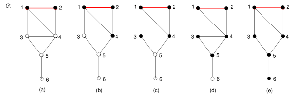
In Figure 1, the edge marked in red in graph is an edge-forcing set. At the first time step, vertex 2 forces vertex 4, at second time step, vertex 1 forces vertex 3, at third time step, vertex 3 or 4 forces vertex 5, in the fourth time step, vertex 5 forces vertex 6.
Edge-forcing set ensures more reliability in the system. For example, the PMUs placed adjacent to each other in an electrical system can be used as backup servers so that if one becomes faulty, the adjacent PMU can support the system, thereby monitoring the entire system without any interruption.
2 Complexity of edge-forcing problem
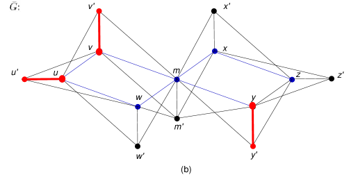
In this section we prove that edge-forcing problem is NP-complete. The reduction will be from the NP-completeness of zero forcing problem [6]. Let be a graph. For , let denote the open neighborhood of in . Then construct the graph as follows. The vertex set , where . The edge set , where and and . See Figure 2.
![[Uncaptioned image]](/html/2108.04764/assets/x2.png)
Lemma 2.1
If is an edge-forcing set of , then there exists an edge-forcing set of with , such that .
Proof 2.2
We have the following two cases.
Case 1: If , then .
Case 2: If , then may contain edges from as well as . Suppose contains an edge . Then replace the edge in with , since the vertices force all the vertices which the vertices would force. Suppose contains an edge . Then replace the edge in with either or , since the vertices or force all the vertices which the vertices would force. The final set of edges thus obtained on replacing edges of with the respective edges in , is taken as . Clearly is an edge-forcing set of with and .
Now we can prove the essential part for our reduction.
Lemma 2.3
Every zero forcing set of induces an edge-forcing set of of the same cardinality and conversely.
Proof 2.4
Suppose is a zero forcing set of . Considering the edge set in , if forces a vertex in , then in initially forces , after which forces . Thus the vertices force the vertices in . It is clear that vertices of set iteratively force all the vertices of . Hence is an edge-forcing set of .
Conversely, suppose is an edge-forcing set of . By Lemma 2.1 we can obtain a set which is an edge-forcing set of . Consider vertex set in . If the vertices force the vertices in , it is evident that forces the vertex in . Hence is a zero forcing set of .
Note that Lemma 2.2 also implies that is a minimum zero forcing set of if and only if is a minimum edge-forcing set of . Combining this result with the fact that the graph can clearly be constructed from in polynomial time, we arrive at the following main result.
Theorem 2.5
The edge-forcing problem is NP-complete.
3 Butterfly networks
Interconnection network is a connection pattern of the components in a system. This is necessary for fast and trusted communication among systems in any parallel computer. The development of large scale integrated circuit technology has led to the growth of complex interconnection networks [23]. Graph Theory is used in the analysis and design of these complex networks [24].
An interconnection network is characterised as a model in graph theory where vertices and edges are represented by devices and their communication links respectively. In a multistage network, inputs are connected to outputs. The butterfly network is an important multistage interconnection network which has an attractive architecture for communication [25]. It overcomes few of the disadvantages of the hypercube, which is the standard network used in industries. Some of its advantages are high bandwidth, small diameter and constant degree switches. Butterfly networks are used to perform a method to demonstrate fast fourier transform used in the area of signal processing [26].
Definition 3.1
[26] The -dimensional butterfly network , has a vertex set and vertices and are connected if and either or and differ precisely in the bit.
Remark 3.2
The vertices are said to be at Level , . If the end vertices of and of an edge satisfy the condition that , then the edge is called a straight edge. Otherwise the edge is called a cross edge. It is customary to write the binary sequence as a decimal number.
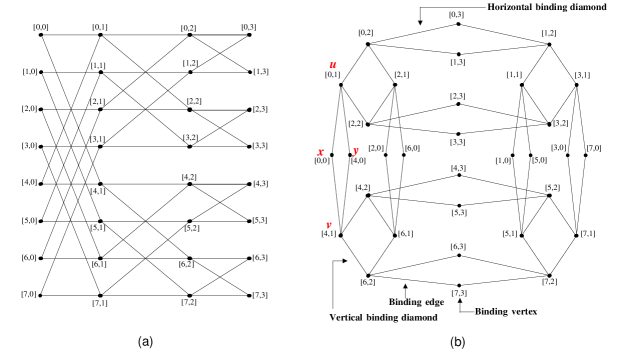
An efficient representation for butterfly network has been obtained by Manuel et al., [25]. The butterfly network in Figure 3(a) is the normal representation; an alternative representation, called the diamond representation, is given in Figure 3(b). By a diamond we mean a cycle of length 4. Two nodes and in are said to be mirror images of each other if and differ precisely in the first bit. The removal of Level 0 vertices of gives two subgraphs and of , each isomorphic to . Since is a vertex-cut of , the vertices are called binding vertices of . If a 4-cycle in has binding vertices then it is called a binding diamond. The edges of binding diamonds are called binding edges. Such diamonds are also obtained when vertices of at Level are removed. To distinguish between the two, we call the binding diamonds defined by removing the vertices at Level 0 as vertical binding diamonds and those defined by removing vertices at Level as horizontal binding diamonds. The two types of diamonds are shown in Figure 3(b).
4 Edge-forcing in butterfly networks
For determining a lower bound for the edge-forcing number in butterfly networks we consider the diamond representation of , and for the actual computation of edge-forcing number, we consider the normal representation. We observe that when is even, the number of levels in is odd and vice versa.
Theorem 4.1
The edge-forcing set does not exist for .
Proof 4.2
There are four edge disjoint 4-cycles in . If none of the edges in a 4-cycle is present in an edge-forcing set, then both vertices of degree 2 in the 4-cycle cannot be forced by any edge in the edge-forcing set. Hence every 4-cycle contributes an edge to the forcing set. See Figure 4. Choice of these independent edges cannot force the left out vertices of degree 2. Hence one more edge is required in the forcing set but this induces a path of length 2 in the forcing set, a contradiction.

Lemma 4.3
The edge-forcing number of , is at least .
Proof 4.4
Consider a binding diamond of . Assume that none of the edges of belongs to an edge-forcing set of . Let and be the binding vertices of degree 2 in . Both and are adjacent to two vertices and of degree 4 in . For illustration, see Figure 3(b). Hence even if and are forced, both and cannot be forced. Hence at least one edge of should be present in the forcing set. There are binding diamonds in , . Hence .
Determining , has proved to be very challenging. In this section, for and 5 have been determined. Using the recursive nature of , an upper bound has been derived for all . It is also conjectured that this upper bound is the exact value of .
We begin with an algorithm to determine .
Edge-forcing Algorithm :
Input: , the butterfly network of dimension 3
Algorithm:
Step 1: Choose the edges , ;
Step 2: Choose the edges ([2,2], [6,3]), ([3,2], [7,3]), ([0,3], [4,2]), ([1,3], [5,2]) from Levels 2 and 3.
Output: An edge-forcing set having cardinality 8
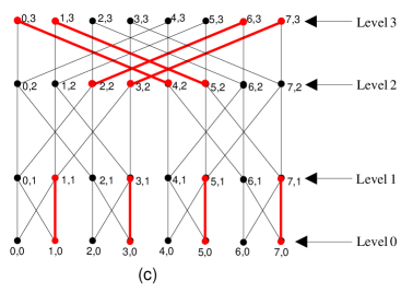
Proof of Correctness:
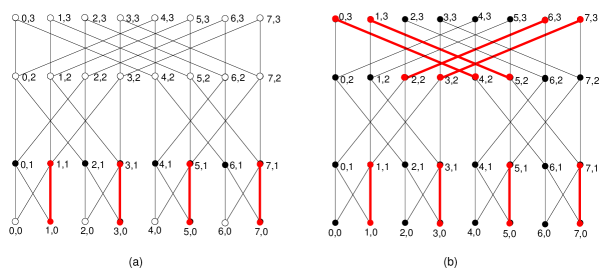
The selected edges between Level 0 and Level 1 force all vertices of Level 1. See Figure 5(a). The edges chosen between Levels 2 and 3 force all vertices of Level 2. See Figure 5(b). Thus in the first step, all vertices of Level 1 are forced. In the second step of the forcing process, the left out vertices of are forced. Figure 5(c) illustrates the edge-forcing of and also the different Levels in a butterfly network.
By edge-forcing algorithm , . Combining this with Lemma 4.2, we have the following result.
Theorem 4.5
The edge-forcing number of is , that is .
We next compute the edge-forcing number of .
Lemma 4.6
The edge-forcing number of is at least , that is .
Proof 4.7
There are 16 binding diamonds in . 16 edges are chosen, one edge from every binding diamond as in the Lemma 4.2. This leaves all vertices in Levels 1 and 3 forced. Level 0 has 8 unforced vertices. The parallel edges connecting vertices of Level 1 and Level 2 are partitioned into 4 subsets and of 4 edges each, where end vertices of edges in are labelled , , , , . An edge chosen with one end in Level 1 and another end in Level 2 in any , does not force any of the 8 unforced vertices in Level 0. But a pair of edges in , forces 2 vertices of the corresponding vertices at Level 0. Thus to force vertices at Level 0, 8 edges are necessary in the edge-forcing set. There are vertices in Level 2 which are yet to be forced, hence at least one more edge has to be chosen in the edge-forcing set. Therefore .
Edge-forcing Algorithm :
Input: , the butterfly network of dimension 4
Algorithm:
Step 1: Choose the edges and the edges , ;
Step 2: Choose the edges and ;
Step 3: Choose the edges and edges ;
Step 4: Select edge ([3,3], [7,2]).
Output: An edge-forcing set having cardinality 25
![[Uncaptioned image]](/html/2108.04764/assets/x8.png)
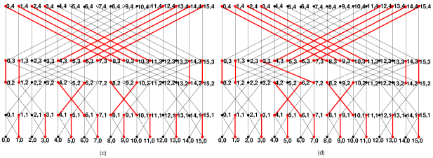
Proof of Correctness:
In Step 1, we have chosen 16 binding edges of , one from each binding diamond. The edges selected in Step 1 force all vertices in Levels 1 and 3. See Figure 6(a). The edges selected using Step 2 and 3 force the remaining 8 vertices in Level 0. See Figure 6(b) and Figure 6(c). Any edge between the end vertices in Levels 2 and 3 will force all the remaining unforced vertices in Levels 2 and 4. See Figure 6(d).
By edge-forcing algorithm , . Combining this with Lemma 4.4, we have the following result.
Theorem 4.8
The edge-forcing number of is , that is .
We now consider , where .
Lemma 4.9
The edge-forcing number of is at least , that is .
Proof 4.10
There are 32 binding diamonds in . 32 edges are chosen, one edge from every binding diamond as in Lemma 4.2. This leaves all vertices in Level 1 and Level 4 forced. Level 0 has 16 unforced vertices. The parallel edges connecting vertices of Level 1 and Level 2 are partitioned into 8 subsets and ,…, of 4 edges each, where end vertices of edges in are labelled , , , , . Choosing an edge with one end in Level 1 and another end in Level 2 in any , does not force any of the 8 unforced vertices in Level 0. But pairs of edges in , force 2 vertices of the corresponding vertices at Level 0. This accounts for an additional 12 edges in the edge-forcing set. Since all the vertices in the higher levels are already forced, only 3 edges are necessary from to force the remaining vertices. Therefore .
Edge-forcing Algorithm :
Input: , the butterfly network of dimension 5
Algorithm:
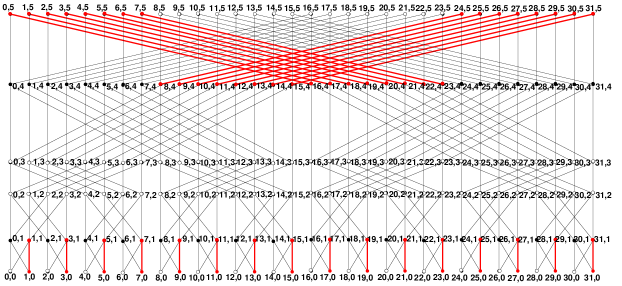
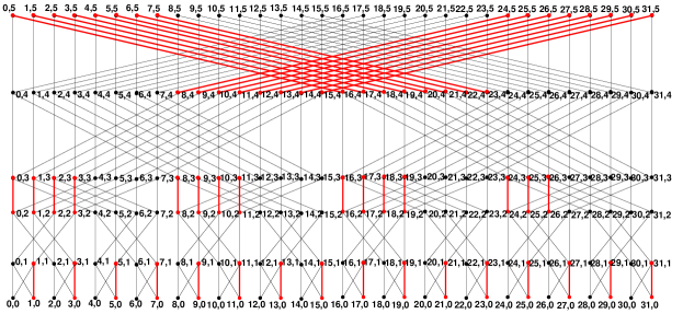
Step 1: Choose the edges , and edges , ;
Step 2: Choose the edges , , , .
Output: An edge-forcing set having cardinality 47
Proof of Correctness:
In Step 1, we have chosen 32 binding edges of , one from each of the binding diamonds. The edges selected using Step 1 force all the vertices in Level 1 and Level 4. See Figure 7. The 15 edges chosen in Levels 2 and 3 by Step 2 are sufficient to force all vertices in Levels 2 and 3 and in turn all vertices in Levels 0 and 5. See Figure 8.
By edge-forcing algorithm , . Combining this with Lemma 4.6, we have the following result.
Theorem 4.11
The edge-forcing number of is , that is .
Now, we will prove the upper bound of the edge-forcing number of , .
Lemma 4.12
For odd, , .
Proof 4.13
The result is true for = 3 and 5 by Theorems 4.3 and 4.7 respectively. For , odd, contains 4 vertex disjoint copies of induced by vertices in Level 0 to Level . The edges in the subgraph induced by vertices in Level and Level are not adjacent to any edge in the four isomorphic copies of . Hence using recursion,
Thus and odd.
Combining Lemma 4.2 with Lemma 4.8, we arrive at the following result.
Theorem 4.14
For , odd, .
Lemma 4.15
For , even, .
Proof 4.16
By Theorem 4.5, the result is true for = 4. For , even, contains four vertex disjoint copies of induced by vertices in Level 0 to Level . The edges in the subgraph induced by vertices in Level and Level are not adjacent to any edge in the four isomorphic copies of . Hence using recursion,
Thus and even.
Combining Lemma 4.2 with Lemma 4.10, we arrive at the following result.
Theorem 4.17
For , even, .
5 Conclusion
In this paper, we have introduced the edge-forcing problem in line with ‘total forcing’, ‘connected forcing’ and ‘-forcing’ studied by various authors. We have established the NP-completeness of the edge-forcing problem. We have obtained a lower bound for the edge-forcing number of butterfly networks , . Further, we have proved that this lower bound is sharp for , = 3, 4, 5 and have obtained an upper bound for higher dimensions. Determining edge-forcing number for higher dimensions of butterfly networks is a challenging open problem.
Acknowledgments
The authors thank Mr. Andrew Arokiaraj for his insightful comments on the computational complexity of the problem. Further, the authors would like to thank the anonymous reviewers for their detailed comments which has helped us to improve the paper to a great extent. The work of R. Sundara Rajan is partially supported by Project No. 2/48(4)/ 2016/NBHM-R&D-II/11580, National Board of Higher Mathematics (NBHM), Department of Atomic Energy (DAE), Government of India.
References
- [1] Benson KF, Ferrero D, Flagg M, Furst V, Hogben L, Vasilevska V, Wissman B. Power domination and zero forcing. arXiv: 1510.02421, 2015.
- [2] Ferrero D, Grigorious C, Kalinowski T, Ryan J, Stephen S. Minimum rank and zero forcing number for butterfly networks. Journal of Combinatorial Optimization, 2019. 37:970–988. doi:10.1007/s10878-018-0335-1.
- [3] Group AMRSGW. Zero forcing sets and the minimum rank of graphs. Linear Algebra and its Applications, 2008. 428:1628–1648. doi:10.1016/j.laa.2007.10.009.
- [4] Burgarth D, Giovannetti V. Full control by locally induced relaxation. Physical Review Letters, 2007. 99(10):100501. doi:10.1103/PhysRevLett.99.100501.
- [5] Burgarth D, Maruyama K. Indirect Hamiltonian identification through a small gateway. New Journal of Physics, 2009. 11:103019. doi:10.1088/1367-2630/11/10/103019.
- [6] Fallat S, Meagher K, Yang B. On the complexity of the positive semidefinite zero forcing number. Linear Algebra and its Applications, 2016. 491:101–122. doi:10.1016/j.laa.2015.03.011.
- [7] Rashidi S, Poursalavati NS, Tavakkoli M. Computing the zero forcing number for generalized Petersen graphs. Journal of Algebra Combinatorics Discrete Structures and Applications, 2019. 7(2):183–193. doi:10.13069/jacodesmath.729465.
- [8] Row DD. Zero forcing number, path cover number, and maximum nullity of cacti. Involve: A Journal of Mathematics, 2011. 4:277–291. doi:10.2140/involve.2011.4.277.
- [9] Davila R, Kenter F. Bounds for the Zero Forcing Number of Graphs with Large Girth. Theory and Applications of Graphs, 2015. 2. doi:10.20429/tag.2015.020201.
- [10] Kalinowski T, Kamcev N, Sudakov B. The Zero Forcing Number of Graphs. SIAM Journal of Discrete Mathematics, 2019. 33:95–115. doi:10.1137/17M1133051.
- [11] Anitha J. Zero Forcing in Snake Graph. International Journal of Recent Technology and Engineering, 2019. 7:133–136. ISSN:2277-3878.
- [12] Eroh L, Kang CX, Yi E. A comparison between the Metric Dimension and Zero Forcing Number of Line Graphs. arXiv:1207.6127v1 [math.CO] 25 Jul 2012.
- [13] Hayat S, Siddiqui HMA, Imran M, Ikhlaq HM. On the zero forcing number and propagation time of oriented graphs. AIMS Press, 2021. 6(2):1833–1850. doi: 10.3934/math.2021111.
- [14] Vatandoost E, Ramezani F, Alikhan S. On the zero forcing number of generalized Sierpinski graphs. Transactions on Combinatorics, 2019. 8:41–50.
- [15] Stephen S. Zero Forcing and Power Domination in Graphs. PhD thesis, The University of Newcastle, Australia, 2017.
- [16] Hogben L, Huynh M, Kingsley N, Meyer S, Walker S, Young M. Propagation time for zero forcing on a graph. Discrete Applied Mathematics, 2012. 160(13-14):1994–2005. doi:10.1016/j.dam.2012.04.003.
- [17] Davila R, Henning MA. On the total forcing number of a graph. Discrete Applied Mathematics, 2019. 257:115–127. doi:10.1016/j.dam.2018.09.001.
- [18] Haynes TW, Hedetniemi SM, Hedetneimi ST, Henning MA. Domination in graphs applied to electric power networks. SIAM Journal on Discrete Mathematics, 2002. 15(4):519–529. doi:10.1137/ S0895480100375831.
- [19] Davila R, Henning MA, Magnant C, Pepper R. Bounds on the Connected Forcing Number of a Graph. Graphs and Combinatorics, 2018. 34(6):1159–1174. doi:10.1007/s00373-018-1957-x.
- [20] Ferrero D, Varghese S, Vijayakumar A. Power domination in honeycomb networks. Journal of Discrete Mathematical Sciences and Cryptography, 2011. 14(6):521–529. doi:10.1080/09720529.2011.10698353.
- [21] Amos D, Caro Y, Randy Davila RP. Upper bounds on the k-forcing number of a graph. arXiv:1401.6206 [math.CO].
- [22] Davila R, Henning MA. On the Total Forcing Number of a Graph. arXiv:1702.06035v3 [math.CO] 27 Feb 2017.
- [23] Konstantinidou S. The selective extra stage butterfly. IEEE Transactions on Very Large Scale Integration Systems, 1993. 1:167–171. doi:10.1109/92.238419.
- [24] Shrinivas SG, Vetrivel S, Elango NM. Applications of graph theory in computer science-An overview. International Journal of Engineering Science and Technology, 2010. 2:4610–4621. ID:15834618.
- [25] Manuel PD, Rajan B, Rajasingh I, Beulah PV. Improved bounds on the crossing number of butterfly network. Journal of Discrete Mathematics and Theoretical Computer Science, 2013. 15(2):87–94. doi:10.46298/dmtcs.611.
- [26] Rajasingh I, Rajan B, Arockiamary ST. Irregular total labeling of butterfly and Benes networks. Irregular total labeling of butterfly and Benes networks, 2011. 253:284–293. doi:10.1007/978-3-642-25462-8_25.