Some specific wormhole solutions in $f(R)$-modified gravity theory

Abstract

The paper deals with the static spherically symmetric wormhole solutions in $f(R)$-modified gravity theory with anisotropic matter field and for some particular choices for the shape functions. The present work may be considered as an extension of the general formalism in r15 for finding wormhole solutions. For isotropic matter distribution it has been shown that wormhole solutions are possible for zero tidal force and it modifies the claim in r17 . Finally energy conditions are examined and it is found that all energy conditions are satisfied in a particular domain with a particular choice of the shape function.

I Introduction:

In astrophysics, there is a popular concept, namely interstellar travel which is commonly described by traversable wormhole r1 . The basic property for the traversability of such wormhole is that they do not possess any horizon, it has throat (having minimum surface area) with a flare-out condition r1.1 as a consequence there is a violation of null energy condition (NEC) by the matter stress tensor at the throat. In spherical polar coordinate in the background of spherically symmetric, spacetime the traversable wormhole is described by the standard line element r2

$$ds^{2}=-e^{2\Phi(r)}dt^{2}+\left[1-\frac{b(r)}{r}\right]^{-1}dr^{2}+r^{2}(d\theta^{2}+sin^{2}\theta d\phi^{2}),$$ (1)

where $\Phi(r)$ is the gravitational redshift function and $b(r)$ is the shape function indicative of the shape of the wormhole throat. The radial co-ordinate ‘$r$’ decreases from infinity to a minimum value $r_{0}$, where $b(r_{0})=r_{0}$ and then increases from $r_{0}$ back to infinity. Here, in order for the wormhole to be traversable, one should avoid the formation of an event horizon r3 which are identified as the surface s with infinite redshift i.e. $e^{2\Phi}\longrightarrow 0$ at the horizon, so that $\Phi(r)$ must be finite everywhere for traversability. Also a fundamental property of wormholes is the flaring out of the throat, which is translated by the condition $(b-b^{\prime}r)/b^{2}>0$ at $r=r_{0}$ r4 . At the throat, the condition $b^{\prime}(r_{0})<1$ is imposed in order to have wormhole solutions r4 -r5 . It is well known that wormholes in classical general relativity require a violation of the null energy condition, and the corresponding matter is termed as “exotic matter” r6 . Such matter must be confined to a very narrow band around the throat.

However, recently it has been shown in the context of modified theories of gravity that the matter threading the wormhole may satisfy the energy conditions but the effective stress-energy tensor r7 involving higher order derivatives is responsible for the violation of the NEC. There are several wormhole solutions in modified gravity theories, for examples, in Brane-world gravity wormhole solutions are obtained by various technique b1 –b5 , in Einstein-Gauss-Bonnet gravity, traversable wormhole solutions n1 –n2 satisfy weak energy conditions, in $f(R,T)$ gravity theory, thin-shell wormhole solutions n3 –n7 are obtained for suitable choice of ‘$f$’ and it is found that these solutions satisfy both null and weak energy conditions n8 –n9 , in Scalar-Tensor gravity traversable and spinning wormholes are found in the literature n10 –n11 while in Lovelock gravity theory various wormholes (i.e. Lorentzian, Cosmological and Classical) are obtained n12 –n14 .

Over the past decade, $f(R)$ gravity theory has been extensively studied as one of the simplest modifications to Einstein-Hilbert action. In this modified gravity theory, wormhole geometries and some exact solutions are obtained n15 by various choices of the function ‘$f$’. It is found that for the above wormhole solutions, not only the null energy condition is satisfied, but also weak and dominant energy conditions are also satisfied n16 –n17 . Also, both static and evolving wormhole solutions are obtained in recent past n18 –n19 . In most of these works, viability bounds have been explored for energy conditions considering both imperfect as well as perfect fluid models. Further, wormholes solutions have been constructed in some cases through cut and paste technique.

In this work, $f(R)$-modified gravity theory has been considered for obtaining wormhole solutions both for anisotropic and isotropic matter fields. For anisotropic matter field, wormhole solutions are obtained using the general mechanism in r15 for Einstein gravity. Also, energy conditions are discussed in each case. For isotropic matter field, wormhole solutions so obtained are examined whether they are in favour or against the conclusion in r17 . The paper is organized as follows: Basic equations in $f(R)$-modified gravity theory have been presented in section II. Section III deals with wormhole solutions with anisotropic matter field and energy conditions are examined. In section IV, wormhole solutions are constructed for isotropic matter field, and in section V, embedding diagrams of wormholes are shown. Finally, summary and concluding remarks are given in section VI.

II Basic equations in $f(R)$-modified gravity theory

In $f(R)$-modified gravity, Ricci scalar $R$ is replaced by an arbitrary function $f(R)$ in the Einstein-Hilbert action r8

$$S_{EH}=\int\sqrt{-g}Rd^{4}x$$

becomes :

$$S_{f(R)}=\int\sqrt{-g}f(R)d^{4}x.$$

In $f(R)$ gravity model, action is given by r9

$$S=\frac{1}{2k^{2}}\int d^{4}x\sqrt{-g}f(R)+S_{M}(g^{\mu\nu},\psi)$$ (2)

where $k^{2}=8\pi G$, and for notational simplicity we consider $k^{2}=1$ in this work. $S_{M}(g^{\mu\nu},\psi)$ is the matter action, defined as $S_{M}=\int d^{4}x\sqrt{-g}\mathcal{L}_{M}(g_{\mu\nu},\psi)$, where $\mathcal{L}_{M}$ is the matter Lagrangian density, where matter is assumed to be minimally coupled to gravity and $\psi$ collectively denotes the matter fields.

Now, the corresponding field equations in the metric approach (varying the action with respect to $g^{\mu\nu}$) yields n18 ,r11 -r12 ,

$$F(R)R_{\mu\nu}-\frac{1}{2}f(R)g_{\mu\nu}-\nabla_{\mu}\nabla_{\nu}F(R)+g_{\mu\nu}\Box F(R)=T^{m}_{\mu\nu}$$ (3)

where $F=\frac{df}{dR}$ , $\Box=\nabla_{\mu}\nabla^{\mu}$, $R_{\mu\nu}$ is the Ricci tensor, and $T^{m}_{\mu\nu}$ is the energy momentum tensor. After the contraction of equation (3), we obtain the following relation

$$FR-2f+3\Box F=T.$$ (4)

Using equation (4) in (1), we get the standard form of Einstein field equations as

$$G_{\mu\nu}=R_{\mu\nu}-\frac{1}{2}Rg_{\mu\nu}=T_{\mu\nu}^{\text{eff}}=T_{\mu\nu}^{(g)}+T_{\mu\nu}^{m}/F,$$ (5)

where $G_{\mu\nu}$ is the Einstein tensor, $T_{\mu\nu}^{\text{eff}}=T_{\mu\nu}^{(g)}+T_{\mu\nu}^{m}/F$ is the effective energy-momentum tensor and $T_{\mu\nu}^{(g)}$, due to gravity is given by

$$T_{\mu\nu}^{(g)}=\frac{1}{F}\left[\nabla_{\mu}\nabla_{\nu}F-\frac{1}{4}g_{\mu\nu}(RF+\Box F+T)\right].$$ (6)

To obtain some particular wormhole solution, we assume that the stress-energy momentum tensor that threads the wormhole is given by an anisotropic matter distribution as r13

$$T_{\mu\nu}=(\rho+p_{t})u_{\mu}u_{\nu}+p_{t}g_{\mu\nu}+(p_{r}-p_{t})v_{\mu}v_{\nu},$$

where $v^{\mu}$ is the unit spacelike vector in the radial direction, $u^{\mu}$ is the four velocity vector, $\rho(r)$ is the energy density, $p_{r}(r)$ is the radial pressure measured in the direction of $v^{\mu}$, and $p_{t}(r)$ is the transverse pressure measured in the orthogonal direction to $v^{\mu}$. We shall take the redshift function to be constant which helps to investigate interesting wormhole solutions.

Thus, for the wormhole metric (1), the explicit form of effective field equations (5) gives r13

$$\frac{\rho}{F}+\frac{J}{F}=\frac{b^{\prime}}{r^{2}},$$ (7)

$$\frac{p_{r}}{F}+\frac{1}{F}\left[\left(1-\frac{b}{r}\right)\left(F^{\prime\prime}-F^{\prime}.\frac{b^{\prime}r-b}{2r^{2}(1-b/r)}\right)-J\right]=-\frac{b}{r^{3}},$$ (8)

$$\frac{p_{t}}{F}+\frac{1}{F}\left[\left(1-\frac{b}{r}\right)\frac{F^{\prime}}{r}-J\right]=-\frac{b^{\prime}r-b}{2r^{3}},$$ (9)

where the prime denotes a derivative with respect to the radial co-ordinate ‘$r$’. The term $J=J(r)$ is defined as

$$J(r)=\frac{1}{4}(FR+\Box F+T),$$ (10)

for notational simplicity. The curvature scalar, $R$ is given by

$$R=\frac{2b^{\prime}}{r^{2}},$$ (11)

and $\Box F$ has the following expression:

$$\Box F=\left(1-\frac{b}{r}\right)\left[F^{\prime\prime}-\frac{b^{\prime}r-b}{2r^{2}(1-b/r)}F^{\prime}+\frac{2F^{\prime}}{r}\right].$$ (12)

Now, the gravitational field equations (7)-(9) can be reorganized to yield as follows:

$$\frac{Fb^{\prime}}{r^{2}}=\rho,$$ (13)

$$-\frac{bF}{r^{3}}+\frac{F^{\prime}}{2r^{2}}(b^{\prime}r-b)-F^{\prime\prime}\left(1-\frac{b}{r}\right)=p_{r},$$ (14)

$$-\frac{F^{\prime}}{r}\left(1-\frac{b}{r}\right)+\frac{F}{2r^{3}}(b-b^{\prime}r)=p_{t}.$$ (15)

This set of coupled ordinary differential equations (13)–(15) gives the throat function for a given fluid and for a given $F(r)$. As the above set of differential equations is first order in ‘$b$’ so using the throat condition (i.e. $b(r_{0})=r_{0}$) it is possible to obtain the throat function uniquely.

III Wormhole solutions with anisotropic matter field and energy conditions

We consider the barotropic equation of state $p_{t}=\omega\rho$, related to the tangential pressure and the energy density which provides the following differential equation

$$F^{\prime}(1-\frac{b}{r})-\frac{F}{2r^{2}}\left[b-(1+2\omega)b^{\prime}r\right]=0.$$ (16)

Now, one may deduce $F(r)$ by imposing a specific shape function, and inverting equation (11), i.e. $R(r)$, to find $r(R)$, the specific form of $f(R)$ may be found from trace equation (4). In the following section, we consider several shape functions usually applied in the literature.

III.0.1 Shape function: $b(r)=\frac{r_{0}^{n}}{r^{n-1}}$ for some $n>0$

Let us consider the shape function $b(r)=\frac{r_{0}^{n}}{r^{n-1}}$ for some $n>0$ (in r14 the shape function is considered for $n=2$, here we are considering the general case ). Putting the value of $b(r)$ in equation (16) we obtain

$$F(r)=C_{1}\left(1-\frac{r_{0}^{n}}{r^{n}}\right)^{\frac{n+(n-1)2\omega}{2n}},$$ (17)

where $C_{1}$ is arbitrary constant. The gravitational field equations (13)-(15) give

$$\rho = C_{1}(1-n)\frac{r_{0}^{n}}{r^{n+2}}\left(1-\frac{r_{0}^{n}}{r^{n}}\right)^{\frac{n+(n-1)2\omega}{2n}},$$ (18)

$$p_{r} = -\frac{C_{1}}{2}\frac{1}{r^{2(n+1)}}\left(1-\frac{r_{0}^{n}}{r^{n}}\right)^{\frac{-n+(n-1)2\omega}{2n}}\times\bigg{[}r^{n}\bigg{\{}2-(n+1)(n+(n-1)2\omega)\bigg{\}}$$ (19)

$$+\leavevmode\nobreak\ r_{0}^{n}\bigg{\{}(n+(n-1)2\omega)(n+1+(n-1)\omega)-2\bigg{\}}\bigg{]},$$

$$p_{t} = C_{1}\omega(1-n)\frac{r_{0}^{n}}{r^{n+2}}\left(1-\frac{r_{0}^{n}}{r^{n}}\right)^{\frac{n+(n-1)2\omega}{2n}}.$$ (20)

Now, we have

$$T = -\rho+p_{r}+2p_{t}$$

$$= C_{1}\frac{1}{2}\frac{r_{0}^{n}}{r^{2(n+1)}}\left(1-\frac{r_{0}^{n}}{r^{n}}\right)^{\frac{-n+(n-1)2\omega}{2n}}\times\bigg{[}r^{n}\bigg{\{}n^{2}+2n^{2}\omega+3n+2\omega-4\omega n-4\bigg{\}}$$

$$+\leavevmode\nobreak\ r_{0}^{n}\biggl{\{}4\omega^{2}n-2n^{2}\omega^{2}-3\omega n^{2}-2\omega^{2}-n^{2}-2\omega-3n+5\omega n+4\biggr{\}}\bigg{]},$$ (22)

and using equation(12)

$$\Box F=C_{1}\frac{n+(n-1)2\omega}{2}\frac{r_{0}^{n}}{r^{2(n+1)}}\bigg{[}r_{0}^{n}\biggl{\{}n-1+(n-1)\omega\biggr{\}}+r^{n}(1-n)\bigg{]}.$$ (23)

The Ricci scalar is given by $R=2(1-n)\frac{r_{0}^{n}}{r^{n+2}}$ (using equation (11)) i.e. $r=\left(\frac{2(1-n)r_{0}^{n}}{R}\right)^{\frac{1}{n+2}}$, and hence at the throat we have

$$r_{0}=\left(\frac{2(1-n)}{R_{0}}\right)^{\frac{1}{2}}.$$

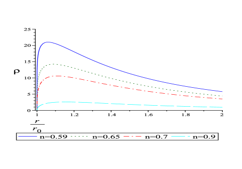
Figure 1: The above figure shows the variations of $\rho$ versus $r/r_{0}$ for $r_{0}=0.1$, $\omega=\frac{1}{2}$, $C_{1}=1$ corresponding to the shape function (1).

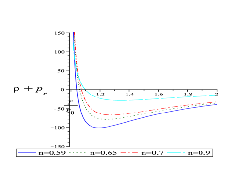
Figure 2: The above figure shows the variations of $\rho+p_{r}$ versus $r/r_{0}$ for $r_{0}=0.1$, $\omega=\frac{1}{2}$, $C_{1}=1$ corresponding to the shape function (1).

After substituting these relations into the equation (4), the specific form of $f(R)$ is finally given by

$$f(R) = \frac{1}{2}C_{1}R\bigg{\{}1-\left(\frac{R}{R_{0}}\right)^{\frac{n}{n+2}}\bigg{\}}^{\frac{-n+(n-1)2\omega}{2n}}\Bigg{[}\left(\frac{R}{R_{0}}\right)^{\frac{n}{n+2}}\biggl{\{}-\frac{3}{2}\frac{n+(n-1)2\omega}{2}(1+\omega)-1$$ (24)

$$-\leavevmode\nobreak\ \frac{1}{4(1-n)}\left(4-2\omega-3n+5\omega n-2\omega^{2}-n^{2}-3\omega n^{2}+4\omega^{2}n-2\omega^{2}n^{2}\right)\biggr{\}}$$

$$+\leavevmode\nobreak\ \biggl{\{}\frac{3}{2}\frac{n+(n-1)2\omega}{2}+1-\frac{1}{4(1-n)}\left(2\omega n^{2}+n^{2}+2\omega+3n-4\omega n-4\right)\biggr{\}}\Bigg{]},$$

as in r13 if we consider $n=2$.

The energy conditions are investigated in terms of principal pressures which are as followsr16 ; r18 :
$\diamond$ Null energy condition (NEC): $\rho+p_{r}\geq 0$, $\rho+p_{t}\geq 0$,
$\diamond$ Weak energy condition (WEC): $\rho\geq 0$, $\rho+p_{r}\geq 0$, $\rho+p_{t}\geq 0$,
$\diamond$ Strong energy condition (SEC): $\rho+p_{r}\geq 0$, $\rho+p_{t}\geq 0$, $\rho+p_{r}+2p_{t}\geq 0$,
$\diamond$ Dominant energy condition (DEC): $\rho\geq 0$, $\rho-|p_{r}|\geq 0$, $\rho-|p_{t}|\geq 0$.

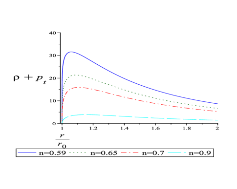
Figure 3: The above figure shows the variations of $\rho+p_{t}$ versus $r/r_{0}$ for $r_{0}=0.1$, $\omega=\frac{1}{2}$, $C_{1}=1$ corresponding to the shape function (1).

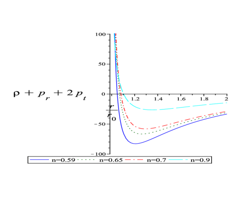
Figure 4: The above figure shows the variations of $\rho+p_{r}+2p_{t}$ versus $r/r_{0}$ for $r_{0}=0.1$, $\omega=\frac{1}{2}$, $C_{1}=1$ corresponding the shape function (1).

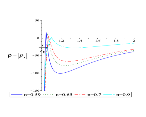
Figure 5: The above figure shows the variations of $\rho-|p_{r}|$ versus $r/r_{0}$ for $r_{0}=0.1$, $\omega=\frac{1}{2}$, $C_{1}=1$, corresponding the shape function (1).

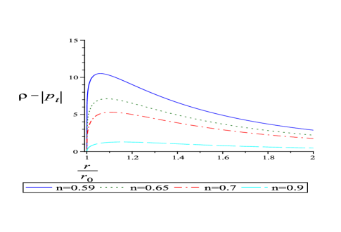
Figure 6: The above figure shows the variations of $\rho-|p_{t}|$ versus $r/r_{0}$ for $r_{0}=0.1$, $\omega=\frac{1}{2}$, $C_{1}=1$, corresponding the shape function (1).

Considering $r_{0}=0.1$, $\omega=\frac{1}{2}$, $C_{1}=1$ we have drawn the graphs $\rho$ (FIG.1), $\rho+p_{r}$ (FIG.2), $\rho+p_{t}$ (FIG.3), $\rho+p_{r}+2p_{t}$ (FIG.4), $\rho-|p_{r}|$ (FIG.5), $\rho-|p_{t}|$ (FIG.6) with respect to $r/r_{0}$ for the above shape function.

III.0.2 Shape function: $b(r)=\frac{r}{1+r-r_{0}},0<r_{0}<1$

Let us consider another shape function $b(r)=\frac{r}{1+r-r_{0}}$, $0<r_{0}<1$ r14 ; r15 . Putting the value of $b(r)$ in equation (16) we obtain

$$F(r)=C_{1}r^{\frac{\omega}{r_{0}}}(r-r_{0})^{-\frac{w}{r_{0}}+\omega+\frac{1}{2}}(1+r-r_{0})^{\omega-\frac{1}{2}},$$ (25)

where $C_{1}$ is arbitrary constant. It is useful to write the equation (25) in the form of

$$F(r)=C_{1}X^{u}Y^{v}Z^{s}$$ (26)

where $C_{1}$ is arbitrary constant, and $X$, $Y$, $Z$, $u$, $v$, $s$ are defined as $X=r$, $Y=(r-r_{0})$, $Z=(1+r-r_{0})$, $u=\frac{\omega}{r_{0}}$, $v=-\frac{w}{r_{0}}+\omega+\frac{1}{2}$, $s=\omega-\frac{1}{2}$.
Then the gravitational field equations (13)-(15) become

$$\rho = C_{1}(1-r_{0})X^{u-2}Y^{v}Z^{s-2},$$ (27)

$$p_{r} = -C_{1}\Bigg{[}X^{u-2}Y^{v}Z^{s-1}+\frac{u}{2}X^{u-1}Y^{v}Z^{s-2}+\frac{v}{2}X^{u}Y^{v-1}Z^{s-2}+\frac{s}{2}X^{u}Y^{v}Z^{s-3}$$ (28)

$$+\leavevmode\nobreak\ u(u-1)X^{u-2}Y^{v+1}Z^{s-1}+v(v-1)X^{u}Y^{v-1}Z^{s-1}+s(s-1)X^{u}Y^{v+1}Z^{s-3}$$

$$+\leavevmode\nobreak\ 2uvX^{u-1}Y^{v}Z^{s-1}+2usX^{u-1}Y^{v+1}Z^{s-2}+2vsX^{u}Y^{v}Z^{s-2}\Bigg{]},$$

$$p_{t} = \omega C_{1}(1-r_{0})X^{u-2}Y^{v}Z^{s-2}.$$ (29)

Now, we have

$$T = -\rho+p_{r}+2p_{t}$$ (30)

$$= C_{1}\Bigg{[}(2\omega-1)(1-r_{0})X^{u-2}Y^{v}Z^{s-2}-X^{u-2}Y^{v}Z^{s-1}-\frac{u}{2}X^{u-1}Y^{v}Z^{s-2}-\frac{v}{2}X^{u}Y^{v-1}Z^{s-2}$$

$$-\leavevmode\nobreak\ \frac{s}{2}X^{u}Y^{v}Z^{s-3}-u(u-1)X^{u-2}Y^{v+1}Z^{s-1}-v(v-1)X^{u}Y^{v-1}Z^{s-1}-s(s-1)X^{u}Y^{v+1}Z^{s-3}$$

$$-\leavevmode\nobreak\ 2uvX^{u-1}Y^{v}Z^{s-1}-2usX^{u-1}Y^{v+1}Z^{s-2}-2vsX^{u}Y^{v}Z^{s-2}\Bigg{]},$$

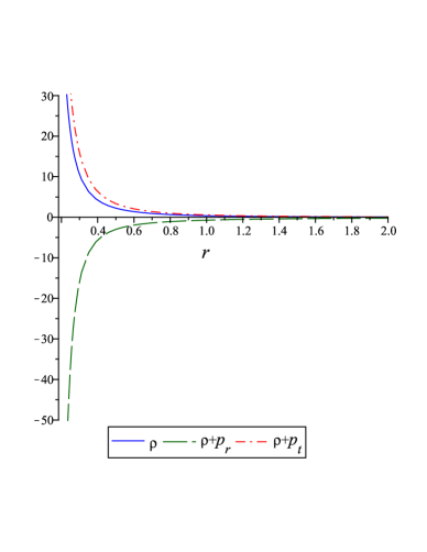
Figure 7: Variation of $\rho$ (solid curve), $\rho+p_{r}$ (longdashed curve) and $\rho+p_{t}$ (dashdot curve) for $C_{1}=1$, $r_{0}=0.1$, $\omega=1/2$ corresponding to the shape function (2).

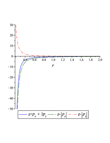
Figure 8: Variation of $\rho+p_{r}+2p_{t}$ (solid curve), $\rho-|p_{r}|$ (longdashed curve) and $\rho-|p_{t}|$ (dashdot curve) for $C_{1}=1$, $r_{0}=0.1$, $\omega=1/2$ corresponding to the shape function (2).

and using equation(12)

$$\Box F = C_{1}\Bigg{[}u(u-1)X^{u-2}Y^{v+1}Z^{s-1}+v(v-1)X^{u}Y^{v-1}Z^{s-1}+s(s-1)X^{u}Y^{v+1}Z^{s-3}+2uvX^{u-1}Y^{v}Z^{s-2}$$ (31)

$$+\leavevmode\nobreak\ 2usX^{u-1}Y^{v+1}Z^{s-2}+2vsX^{u}Y^{v}Z^{s-2}+\frac{u}{2}X^{u-1}Y^{v-1}Z^{s-1}+\frac{v}{2}X^{u}Y^{v-2}Z^{s-1}$$

$$+\leavevmode\nobreak\ \frac{s}{2}X^{u}Y^{v-1}Z^{s-2}+2uX^{u-2}Y^{v}Z^{s}+2vX^{u-1}Y^{v-1}Z^{s}+2sX^{u-1}Y^{v}Z^{s-1}\Bigg{]}.$$

The Ricci scalar is given by $R=2(1-r_{0})X^{-2}Z^{-2}$ (using equation (11)). After substituting these relations into the equation (4), the specific form of $f(r)$ is finally given by

$$f(r) = C_{1}\Bigg{[}4u(u-1)X^{u-2}Y^{v+1}Z^{s-1}+(8uv+6s)X^{u-1}Y^{v}Z^{s-1}+8usX^{u-1}Y^{v+1}Z^{s-2}+8vsX^{u}Y^{v}Z^{s-2}$$ (32)

$$+\leavevmode\nobreak\ 3v(v-1)X^{u}Y^{v-1}Z^{s-1}+4s(s-1)X^{u}Y^{v+1}Z^{s-3}+\frac{3u}{2}X^{u-1}Y^{v-1}Z^{s-1}+\frac{3v}{2}X^{u}Y^{v-2}Z^{s-1}$$

$$+\left(\frac{3s}{2}+v(v-1)\right)X^{u}Y^{v-1}Z^{s-2}+6uX^{u-2}Y^{v}Z^{s}+6vX^{u-1}Y^{v-1}Z^{s}$$

$$+(-2\omega+3)(1-r_{0})X^{u-2}Y^{v}Z^{s-2}+\leavevmode\nobreak\ X^{u-2}Y^{v}Z^{s-1}+\frac{u}{2}X^{u-1}Y^{v}Z^{s-2}$$

$$+\frac{v}{2}X^{u}Y^{v-1}Z^{s-2}+\frac{s}{2}X^{u}Y^{v}Z^{s-2}\Bigg{]}.$$

Using the same value of the parameters as in above, we have drawn the graphs $\rho$, $\rho+p_{r}$ and $\rho+p_{t}$ (FIG.7), $\rho+p_{r}+2p_{t}$, $\rho-|p_{r}|$ and $\rho-|p_{t}|$ (FIG.8) with respect to $r$ for this shape function.

III.0.3 Shape function: $b(r)=re^{-2(r-r_{0})}$

Lastly, let us consider another shape function $b(r)=re^{-2(r-r_{0})}$ r14 . Putting the value of $b(r)$ in equation (16) we obtained

$$F(r)=\left(1-e^{-2(r-r_{0})}\right)^{\omega+\frac{1}{2}}e^{\int\frac{-\omega}{r\left(e^{2(r-r_{0})}-1\right)}dr}.$$ (33)

Then the gravitational field equations (13)-(15) become

$$\rho = \frac{1-2r}{r^{2}}e^{-2(r-r_{0})}\left(1-e^{-2(r-r_{0})}\right)^{\omega+\frac{1}{2}}e^{\int\frac{-\omega}{r\left(e^{2(r-r_{0})}-1\right)}dr},$$ (34)

$$p_{r} = -\rho\bigg{[}\frac{1}{1-2r}+\frac{r^{2}}{(1-2r)}\frac{(1+2\omega)r-\omega}{r\left(e^{2(r-r_{0})}-1\right)}+\bigg{\{}\frac{(1+2\omega)^{2}-2(1+2\omega)e^{2(r-r_{0})}}{\left(e^{2(r-r_{0})}-1\right)^{2}}$$ (35)

$$+\leavevmode\nobreak\ \frac{\omega^{2}+\omega\left((2r+1)e^{2(r-r_{0})}-1\right)}{r^{2}\left(e^{2(r-r_{0})}-1\right)^{2}}-\frac{2(1+2\omega)\omega}{r\left(e^{2(r-r_{0})}-1\right)^{2}}\bigg{\}}\frac{r^{2}e^{2(r-r_{0})}}{(1-2r)}\bigg{]},$$

$$p_{t} = \omega\frac{1-2r}{r^{2}}e^{-2(r-r_{0})}\left(1-e^{-2(r-r_{0})}\right)^{\omega+\frac{1}{2}}e^{\int\frac{-\omega}{r\left(e^{2(r-r_{0})}-1\right)}dr}.$$ (36)

Now, we have

$$T = -\rho+p_{r}+2p_{t}$$ (37)

$$= \bigg{[}(1-2\omega)\frac{1-2r}{r^{2}}e^{-2(r-r_{0})}+\bigg{\{}\frac{-1}{r^{2}e^{2(r-r_{0})}}-\frac{1}{e^{2(r-r_{0})}}\frac{(1+2\omega)r-\omega}{r\left(e^{2(r-r_{0})}-1\right)}+\bigg{\{}\frac{(1+2\omega)^{2}-2(1+2\omega)e^{2(r-r_{0})}}{\left(e^{2(r-r_{0})}-1\right)^{2}}$$

$$+\leavevmode\nobreak\ \frac{\omega^{2}+\omega\left((2r+1)e^{2(r-r_{0})}-1\right)}{r^{2}\left(e^{2(r-r_{0})}-1\right)^{2}}-\frac{2(1+2\omega)\omega}{r\left(e^{2(r-r_{0})}-1\right)^{2}}\bigg{\}}\left(1-e^{-2(r-r_{0})}\right)\bigg{\}}\bigg{]}F(r),$$

and using equation(12)

$$\Box F = \bigg{[}\bigg{\{}\frac{(1+2\omega)^{2}-2(1+2\omega)e^{2(r-r_{0})}}{\left(e^{2(r-r_{0})}-1\right)^{2}}+\frac{\omega^{2}+\omega\left((2r+1)e^{2(r-r_{0})}-1\right)}{r^{2}\left(e^{2(r-r_{0})}-1\right)^{2}}-\frac{2(1+2\omega)\omega}{r\left(e^{2(r-r_{0})}-1\right)^{2}}\bigg{\}}$$ (38)

$$\leavevmode\nobreak\ \left(1-e^{-2(r-r_{0})}\right)+\frac{\left((1+2\omega)r-\omega\right)}{r\left(e^{2(r-r_{0})}-1\right)}\frac{\left(-r+2(\left(e^{2(r-r_{0})}-1\right))\right)}{re^{2(r-r_{0})}}\bigg{]}F(r).$$

Now, Ricci scalar is given by $R=\frac{2(1-2r)e^{2(r-r_{0})}}{r^{2}}$ (using equation(11)). After substituting these relations into the relation (4), the specific form of $f(r)$ is finally given by

$$f(r) = \frac{1}{2}\bigg{[}\frac{2(1-2r)e^{2(r-r_{0})}}{r^{2}}+2\bigg{\{}\frac{(1+2\omega)^{2}-2(1+2\omega)e^{2(r-r_{0})}}{\left(e^{2(r-r_{0})}-1\right)^{2}}+\frac{\omega^{2}+\omega\left((2r+1)e^{2(r-r_{0})}-1\right)}{r^{2}\left(e^{2(r-r_{0})}-1\right)^{2}}$$ (39)

$$-\leavevmode\nobreak\ \frac{2(1+2\omega)\omega}{r\left(e^{2(r-r_{0})}-1\right)^{2}}\bigg{\}}\left(1-e^{-2(r-r_{0})}\right)+\frac{\left((1+2\omega)r-\omega\right)}{r\left(e^{2(r-r_{0})}-1\right)}\frac{\left(-r+2(\left(e^{2(r-r_{0})}-1\right))\right)}{re^{2(r-r_{0})}}$$

$$-\leavevmode\nobreak\ (1-2\omega)\frac{1-2r}{r^{2}}e^{-2(r-r_{0})}+\frac{1}{r^{2}e^{2(r-r_{0})}}+\frac{1}{e^{2(r-r_{0})}}\frac{(1+2\omega)r-\omega}{r\left(e^{2(r-r_{0})}-1\right)}\bigg{]}F(r).$$

FIG.9(A)

FIG.9(B)

FIG.9(C)

FIG.9(D)

FIG.9(E)

FIG.9(F)

Figure 9: Behavior of $\rho$ (FIG.9(A)), $\rho+p_{r}$ (FIG.9(B)), $\rho+p_{t}$ (FIG.9(C)), $\rho+p_{r}+2p_{t}$ (FIG.9(D)), $\rho-|p_{r}|$ (FIG.9(E)) and $\rho-|p_{t}|$ (FIG.9(F)) diagrams have been plotted against $r/r_{0}$ and $\omega$ for shape function(1) when $C_{1}=1$, $-5\leq\omega\leq 5$, $n=0.9$ and $r_{0}=0.1$.

FIG.10(A)

FIG.10(B)

FIG.10(C)

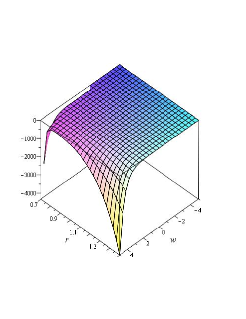
FIG.10(D)

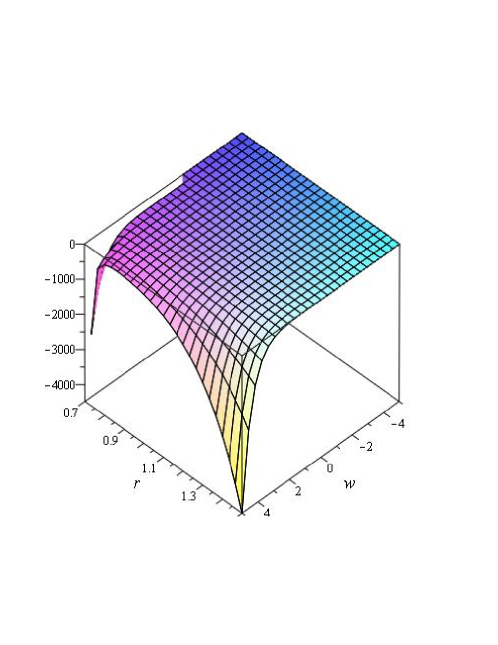
FIG.10(E)

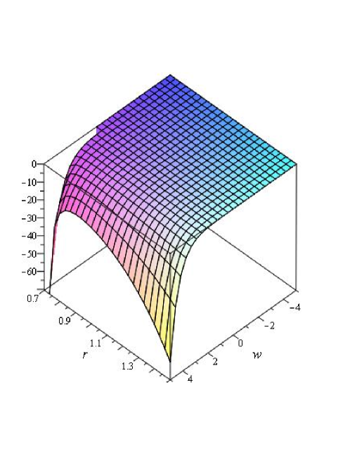
FIG.10(F)

Figure 10: Behavior of $\rho$ (FIG.10(A)), $\rho+p_{r}$ (FIG.10(B)), $\rho+p_{t}$ (FIG.10(C)), $\rho+p_{r}+2p_{t}$ (FIG.10(D)), $\rho-|p_{r}|$ (FIG.10(E)) and $\rho-|p_{t}|$ (FIG.10(F)) diagrams have been plotted against $r$ and $\omega$ for shape function(2) when $C_{1}=1$, $-5\leq\omega\leq 5$ and $r_{0}=0.7$.

We have drawn the 3D figures (Figs.9 and 10) to observe the behavior of $\rho$, $\rho+p_{r}$, $\rho+p_{t}$, $\rho+p_{r}+2p_{t}$, $\rho-|p_{r}|$, $\rho-|p_{t}|$ in the anisotropic scenario for the shape functions (1) and (2), respectively.

IV Isotropic matter field and wormhole solutions in $f(R)$-gravity theory

For the isotropic fluid solutions, we consider $p_{r}=p_{t}=p$. Thus equations (14) and (15) lead to

$$F^{\prime\prime}(r)\left(1-\frac{b(r)}{r}\right)-F^{\prime}\left(\frac{1}{r}+\frac{b^{\prime}(r)}{2r}-\frac{3b(r)}{2r^{2}}\right)+F\left(\frac{3b(r)}{2r^{3}}-\frac{b^{\prime}}{2r^{2}}\right)=0.$$ (40)

Now, for the same choice of shape function (1), $b(r)=\frac{r_{0}^{n}}{r^{n-1}}$ for some $n>0$, the above equation reduces to

$$F^{\prime\prime}\left(\frac{1}{r_{0}^{n}}-\frac{1}{r^{n}}\right)-F^{\prime}\left(\frac{1}{r_{0}^{n}r}-\frac{n+2}{2r^{n+1}}\right)+F\frac{n+2}{2r^{n+2}}=0.$$ (41)

From the equation(41), for $n=2$ we obtain the solution

$$F(r)=C_{1}P\left(\frac{1}{2},\frac{1}{2}\sqrt{17},\sqrt{\frac{-r^{2}+r_{0}^{2}}{r_{0}^{2}}}\right)r^{3/2}+C_{2}Q\left(\frac{1}{2},\frac{1}{2}\sqrt{17},\sqrt{\frac{-r^{2}+r_{0}^{2}}{r_{0}^{2}}}\right)r^{3/2},$$ (42)

where $C_{1}$, $C_{2}$ are arbitrary constants and $P$, $Q$ are Legendre and associated Legendre functions, respectively. Now using equation (13) we get the expression of energy density which is given by

$$\rho=-\frac{r_{0}^{2}}{r^{4}}\Biggl{[}C_{1}P\left(\frac{1}{2},\frac{1}{2}\sqrt{17},\sqrt{\frac{-r^{2}+r_{0}^{2}}{r_{0}^{2}}}\right)r^{3/2}+C_{2}Q\left(\frac{1}{2},\frac{1}{2}\sqrt{17},\sqrt{\frac{-r^{2}+r_{0}^{2}}{r_{0}^{2}}}\right)r^{3/2}\Biggr{]}.$$ (43)

In this case, Ricci scalar is given by $R=-2\frac{r_{0}^{2}}{r^{4}}$ (using equation (11)) i.e. $r=\left(\frac{-2r_{0}^{2}}{R}\right)^{1/4}$, and hence at the throat we have $r_{0}=\left(\frac{-2}{R_{0}}\right)^{1/2}$. Putting these relations in equation (42) provides the form of F(R), which is given by

$$F(R) = C_{1}P\left(\frac{1}{2},\frac{1}{2}\sqrt{17},\sqrt{-\left(\frac{R_{0}}{R}\right)^{1/2}+1}\right)\left(\frac{4}{RR_{0}}\right)^{3/8}$$ (44)

$$+\leavevmode\nobreak\ C_{2}Q\left(\frac{1}{2},\frac{1}{2}\sqrt{17},\sqrt{-\left(\frac{R_{0}}{R}\right)^{1/2}+1}\right)\left(\frac{4}{RR_{0}}\right)^{3/8}.$$

Now we can get the specific form of $f(R)$ from the given integral (existence of the integration is assured from the continuity of the integrand)

$$f(R)=\int_{R_{0}}^{R}F(R)dR.$$ (45)

If we consider the same choice of shape function (2), $b(r)=\frac{r}{1+r-r_{0}}$ , $0<r_{0}<1$, the above equation (40) reduces to

$$F^{\prime\prime}2r^{2}\left(r-r_{0}\right)(1+r-r_{0})-F^{\prime}r(2r^{2}+2r_{0}^{2}+r-2r_{0}-4rr_{0})+F(2+3r-2r_{0})=0.$$ (46)

From the equation (46), we obtain the solution

$$F(r) = C_{1}r^{\frac{\sqrt{r_{0}(r_{0}+1)}+r_{0}}{r_{0}}}G\bigg{(}\frac{-1+r_{0}}{r_{0}},\frac{1}{2}\frac{8(r_{0}(r_{0}+1))^{3}/2+(-9r_{0}-8r_{0}^{2})\sqrt{r_{0}(r_{0}+1)}-2r_{0}}{r_{0}^{3}},$$ (47)

$$\frac{\sqrt{r_{0}(r_{0}+1)}-r_{0}}{r_{0}},\frac{\sqrt{r_{0}(r_{0}+1)}+r_{0}}{r_{0}},\frac{r_{0}+2\sqrt{r_{0}(r_{0}+1)}}{r_{0}},\frac{1}{2},\frac{r}{r_{0}}\bigg{)}$$

$$+\leavevmode\nobreak\ C_{2}r^{\frac{-\sqrt{r_{0}(r_{0}+1)}+r_{0}}{r_{0}}}G\bigg{(}\frac{-1+r_{0}}{r_{0}},\frac{1}{2}\frac{8(r_{0}(r_{0}+1))^{3}/2+(-7r_{0}-8r_{0}^{2})\sqrt{r_{0}(r_{0}+1)}-2r_{0}}{r_{0}^{3}},$$

$$\frac{-\sqrt{r_{0}(r_{0}+1)}+r_{0}}{r_{0}},\frac{-\sqrt{r_{0}(r_{0}+1)}-r_{0}}{r_{0}},\frac{r_{0}-2\sqrt{r_{0}(r_{0}+1)}}{r_{0}},\frac{1}{2},\frac{r}{r_{0}}\bigg{)},$$

where $C_{1}$, $C_{2}$ are arbitrary constants and $G$ is the Heun function. Note that for the third choice of the shape function it is not possible to find $F(r)$ explicitly and hence it is not presented here.

V Embedding diagrams of wormholes

To study the wormhole topology, let us consider the $2D$ hyper surface $\sum$: $t$=constant, $\theta=\pi/2$. The geometry is characterized byr4 ,r20

$$d{S^{2}_{\sum}}=\frac{dr^{2}}{1-\frac{b(r)}{r}}+r^{2}d\phi^{2}.$$ (48)

One may consider this $2D$ hyper surface $\sum$ embedded as rotational surface $z=z(r,\phi)$ into the Euclidean space with metric

$$d{S^{2}_{\sum}}=\left[1+\left(\frac{dz}{dr}\right)^{2}\right]dr^{2}+r^{2}d\phi^{2},$$ (49)

in cylindrical co-ordinates $(r,\phi,z)$. Thus, comparing (48) and (49), one may obtain the expression for embedding function as

$$z(r)=\int_{r_{0}}^{r}\sqrt{\frac{(b/r)}{1-(b/r)}}dr.$$ (50)

Embedding diagrams of wormhole are drawn in FIG.11–FIG.12, considering the mentioned shape functions.

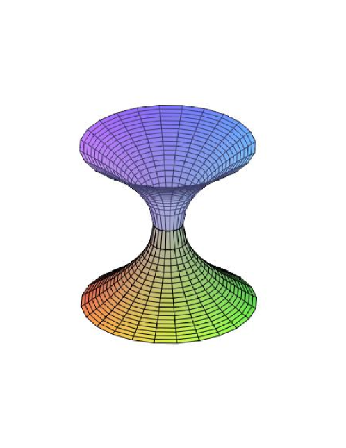
FIG.11(A)

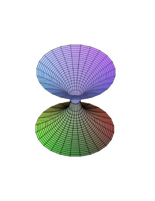
FIG.11(B)

Figure 11: Embedding diagram for the shape function 1 (FIG.11(A)), and for shape function 2 (FIG.11(B)) considering the numerical values $n=0.9$, $r_{0}=0.5$ and $r_{0}=0.5$ for these shape functions, respectively.

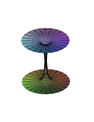
Figure 12: Embedding diagram for the shape function 3 for $r_{0}=0.5$.

VI summary and concluding remarks

This work addresses the following two questions in connection to the formation of traversable wormhole. The first question is that whether the general mechanism developed recently r15 for constructing wormhole solution in Einstein gravity can be extended to $f(R)$-modified gravity theory. The second question is whether the claim in recent past r17 that formation of wormhole with isotropic matter source in Einstein gravity needs non-zero tidal force is true or not in the present $f(R)$-modified gravity theory. Here, three different types of power-law form have been chosen for the shape function and wormhole solutions has been evaluated for anisotropic fluid using the general technique proposed in r15 . It is found that all the energy conditions has been satisfied for the first choice of the shape function in some suitable region of the domain space (in fig.1 to fig.6). For the second choice of the shape function although the energy density is positive but still no energy condition is satisfied (in fig.7 and fig.8). For the third choice of $b(r)$ due to complicated expressions of different energy conditions, it is not possible to infer about their validity. Hence the general technique adopted in r15 can be extended to any modified gravity theory for formation of wormholes.
To address the second question, wormhole solutions for isotropic matter have been constructed for the first two choices of the shape function and vanishing redshift function (i.e. $\phi(r)=0$). Therefore, from the above study, one may conclude that wormhole solutions with isotropic matter field and zero tidal force are possible in modified gravity theory in contrast to Einstein gravity. Further, this new technique for determination of wormhole solution (valid for any gravity theory) helps us to examine whether a typical wormhole geometry is possible in a particular gravity theory or not. Finally, for future work, it would be interesting to examine that such technique of determination of wormhole solution is possible for evolving wormhole geometry.

References

- (1) S. Halder, S. Bhattacharya and S. Chakraborty, Physics Letters B 791, 270-275 (2019).
- (2) Mauricio Cataldo, Luis Leimpi and Pablo Rodriguez, Physics Letters B 757, 130-135 (2016).
- (3) M. Visser, L. Wormholes, From Einstein to Hawking (American Intitute of Physics, New York, 1996).
- (4) Sung-Won KIM, Journal of the Korean Physical Society 10, 63 (2013).
- (5) M. S. Morris, K. S. Throne, Wormholes in spacetime and their use for interstellar travel: a tool for teaching general relativity. Am. J. Phys 56, 395 (1988).
- (6) P. P. Geroch, Topology in general relativity, J. Math. Phys 8, 782 (1967).
- (7) Francisco S. N. Lobo, Wormholes, Warp Drives and Energy Conditions. Springer, 2017.
- (8) Francisco S. N. Lobo, Phantom energy traversable wormholes. Phys. Rev. D 71, 084011 (2005).
- (9) Sung-Won KIM, Journal of the Korean Physical Society 6, 54 (2009).
- (10) Ewa Kocuper, Jery Matyjasek, and Kasia Zwierzchowska. Phys. Rev. D 96, 104057 (2007).
- (11) Ayan Banerjee, P. H. R. S. Moraes, R. A. C. Correa, G. Ribeiro, Wormholes in Randall- Sundrum braneworld, arXiv: 1904.10310[gr-qc].
- (12) Deng Wang, Xin-He Meng, Traversable braneworld wormholes supported by astrophysical observations, Frontiers of Physics 13, 139801(2018).
- (13) F. Parsaei and N. Riazi, New wormhole solutions on the brane, Phys. Rev. D 91, 024015(2015).
- (14) H. S. Tan, On Tidal Love Numbers of Braneworld Black Holes and Wormholes, arXiv:2001.00403[gr-qc].
- (15) F. Parsaei and N. Riazi, Evolving wormhole in the brane-world scenario, arXiv: 2004.01750[gr-qc].
- (16) M. R. mehdizadeh, M. K. Zangeneh and S. N. Lobo, Einstein-Gauss-Bonnet traversable wormholes satisfying the weak energy condition. Phys. Rev. D 91, 084004 (2015).
- (17) M. H. Dehghani, S. H. Hendi, Wormhole Solutions in Gauss-Bonnet-Born-Infeld gravity. Gen. Rel. Gravitation 41, 1853-1863 (2009).
- (18) Z. Yousaf, M. Ilyas and M. Z. Bhatti, Influence of modification of gravity on spherical wormhole models. Modern Physics Letters A 32, 1750163 (2017).
- (19) M. Zubair, S. Waheed and Y. Ahmad, Static spherically symmetric wormholes in gravity. Euro. Phys. J. C 76, 444 (2016).
- (20) M. Z. Bhatti, Z. Yousaf and S. Ashraf, Charged black string thin-shell wormholes in modified gravity. Annals of Physics (2017).
- (21) Z. Yousaf, Construction of charged cylindrical gravastar-like structures. Physics of the Dark Universe 28, 100509 (2020).
- (22) T. Harko, F. S. N. Lobo, S. Nojiri and S. D. Odintsov, gravity. Phys. Rev. D 84, 024020 (2011).
- (23) Sanjay Mandal, Parbati Sahoo, P. K. Sahoo, Wormhole model with a hybrid shape function in gravity, New Astronomy 80, 101421(2020).
- (24) M. Sharif, Iqra Nawazish, Viable wormhole solutions and Noether symmetry in gravity, Annals of Physics 400, 37-63(2019).
- (25) R. Shaikh and S. Kar, Wormholes, the weak energy condition, and scalar-tensor gravity. Phys. Rev. D 94, 024011 (2016).
- (26) X. Y. Chew, B. Kleihaus and J. Kunz, Spinning Wormholes in Scalar-Tensor Theory. arXiv:1802.00365v1[gr-qc] (2016).
- (27) M. H. Dehghani and Z. Dayyani, Lorentzian Wormholes in Lovelock Gravity. arXiv:1802.00365v1[gr-qc] (2016).
- (28) M. R. Mehdizadeh and N. Riazi, Cosmological Wormholes in Lovelock gravity. Phys. Rev. D 85, 124022 (2012).
- (29) G. A. Mena Morugan, Lovelock gravity and classical wormholes. Classical Quantum Gravity 8, 935-946 (1991).
- (30) F. S. N. Lobo and Miguel A. Oliveira, Wormhole geometries in f(R) modified gravity. Phys. Rev. D 80, 104012 (2009).
- (31) N. Godani and Gauranga C. Samanta, Non-violation of energy conditions on wormholes modeling, Mod. Phys. Lett. A 34, 1950226(2019).
- (32) Gauranga C. Samanta and N. Godani, Wormhole modeling supported by non-exotic matter, Mod. Phys. Lett. A 34, 1950224(2019).
- (33) M. Sharif and Z. Zahra, Static wormhole solutions in gravity. Astrophys Space Sci 348, 275-282(2013).
- (34) S. Bhttacharya and S. Chakraborty , gravity solutions for evolving wormholes. Eur.Phys.J.C 77, 558(2017).
- (35) Peter K. F. Kuhfittig, Adv. Studies Theor. Phys 22, 7 (2013).
- (36) Francisco S. N. Lobo, AIP Conference Proceedings 1458, 447 (2012).
- (37) D. Wang and X. Meng, arXiv:1611.01614v1[gr-qc] (2016).
- (38) B. J. Barros and F. S. N. Lobo, Phys. Rev. D 98, 044012 (2018).
- (39) Francisco S. N. Lobo and Miguel A. Oliveira, Wormhole geometries in f(R) modified gravity. Phys. Rev. D 80, 104012 (2009).
- (40) S. Halder, S. Bhattacharya and S. Chakraborty. Modern Physics Letters A 34, 1950095 (2019).
- (41) Gauranga C. Samanta and Nisha Godani. Eur. Phys. J. C 79, 623 (2019).
- (42) A. Sayahian Jahromi, H. Moradpour. International Journal of Modern Physics D 27, 1850024 (2018).
- (43) Mauricio Cataldo and Fabian Orellana, Static phantom wormholes of finite size. Phys. Rev. D 96, 064022 (2017).