Differentiable Subset Pruning of Transformer Heads

Abstract

Multi-head attention, a collection of several attention mechanisms that independently attend to different parts of the input, is the key ingredient in the Transformer. Recent work has shown, however, that a large proportion of the heads in a Transformer’s multi-head attention mechanism can be safely pruned away without significantly harming the performance of the model; such pruning leads to models that are noticeably smaller and faster in practice. Our work introduces a new head pruning technique that we term differentiable subset pruning. Intuitively, our method learns per-head importance variables and then enforces a user-specified hard constraint on the number of unpruned heads. The importance variables are learned via stochastic gradient descent. We conduct experiments on natural language inference and machine translation; we show that differentiable subset pruning performs comparably or better than previous works while offering precise control of the sparsity level.

1 Introduction

The Transformer Vaswani et al. (2017) has become one of the most popular neural architectures used in NLP. Adaptations of the Transformer have been applied to nearly every popular NLP task, e.g. parsing Zhou and Zhao (2019), machine translation Ng et al. (2019), question answering Yang et al. (2019) inter alia. Transformers also form the backbone of state-of-the-art pre-trained language models, e.g. BERT Devlin et al. (2019), GPT-2 Radford et al. (2019) and GPT-3 Brown et al. (2020), that have further boosted performance on various data-driven NLP problems.

The key ingredient in the Transformer architecture is the multi-head attention mechanism, which is an assembly of multiple attention functions Bahdanau et al. (2015) applied in parallel. In practice, each attention head works independently, which allows the heads to capture different kinds of linguistic phenomena Clark et al. (2019); Goldberg (2019); Ettinger (2020); Jawahar et al. (2019). A natural question arises in this context: How many heads does a transformer need?

Michel et al. (2019) offers the insight that a large portion of the Transformer’s heads can be pruned without significantly degrading the test accuracy on the desired task. The experimental evidence behind their claim is a simple greedy procedure that sequentially removes heads. This suggests that a better pruner could reveal that a much larger portion of the heads can be safely removed. To provide a more robust answer to Michel et al.’s question, we build a high-performance pruner and show that their approach itself significantly underestimates the number of Transformer heads that can be pruned away.

From a bird’s eye view, our paper contributes the proposal that Transformer head pruning is best viewed as a subset selection problem. Subset selection is common across many areas of NLP: from extractive summarization Gillenwater et al. (2012) to vowel typology Cotterell and Eisner (2017). In the case of head pruning, the concrete idea is that the user specifies a number of heads $K$ that they would like their Transformer to have depending on their budgetary and other constraints, and then the pruner enforces this constraint. Methodologically, we present a differentiable subset pruner (Fig. 1) that makes use of Gumbel machinery; specifically the Gumbel top-$K$ procedure of Vieira (2014). This construction allows us to relax our pruner into a differentiable sampling routine that qualitatively resembles a discrete analogue of dropout Srivastava et al. (2014); Gal and Ghahramani (2016).

Empirically, we perform experiments on two common NLP tasks: natural language inference (MNLI; Williams et al., 2018) and machine translation (IWSLT2014; Cettolo et al., 2014). We show that our differentiable subset pruning scheme outperforms two recently proposed Transformer head pruners—Michel et al. (2019) and Voita et al. (2019)—on both tasks in terms of sparsity–performance trade-off. Our method recovers a pruned Transformer that has $\approx 80\%$ accuracy on MNLI and $\approx 30$ BLEU score on IWSLT when more than $90\%$ of the heads are removed, which brings about $\approx 33\%$ inference speedup and $\approx 24\%$ model size shrinkage.

Our experiments also suggest several broader conclusions about pruning Transformers. In this paper, we taxonomize existing pruning methods into two pruning paradigms: pipelined pruning and joint pruning. Pipelined pruning consists of two stages: i) training or fine-tuning an over-parameterized model on the target task and ii) pruning the model after training. A number of techniques fall into this category LeCun et al. (1990); Hassibi et al. (1994); Han et al. (2016); Molchanov et al. (2017b). In contrast, joint pruning blends the pruning objective into the training objective by training or fine-tuning the over-parameterized model with a sparsity-enforcing regularizer, sometimes followed up by a trivial post-processing step to arrive at a final sparse model. Kingma et al. (2015) and Louizos et al. (2018) are examples of this kind of pruning. We show that pipelined head pruning schemes, such as that of Michel et al., underperform compared to joint head pruning schemes, such as that of Voita et al. (2019). Our differentiable subset pruner can be adapted to both paradigms and it outperforms prior work in both, especially in high sparsity regions.

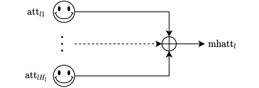
(a) Standard multi-head attention. Attention heads in the same layer $l$ are combined by summation.

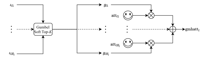
(b) Multi-head attention with differentiable subset pruning. A gate $g_{lh}\in[0,1]$ is applied on each head. The gate values are determined by Gumbel Soft top-$K$ algorithm, which takes the head importance scores $\iota_{lh}$ as inputs. The least "important" heads will have their gate values close to $0$, so they are pruned in effect.

Figure 1: Illustration of gated multi-head attention compared with standard multi-head attention.

2 Background: Multi-head Attention

In this section, we provide a detailed overview of multi-head attention Vaswani et al. (2017) in order to develop the specific technical vocabulary to discuss our approaches for head pruning. We omit details about other parts of the Transformer and refer the reader back to the original work of Vaswani et al. (2017). First, let $\mathbf{z}=z_{1},\ldots,z_{T}$ be a sequence of $T$ real vectors where $z_{t}\in\mathbb{R}^{d}$, and let $q\in\mathbb{R}^{d}$ be a query vector. An attention mechanism is defined as

$$\mathrm{att}(\mathbf{z},q)=W_{o}\sum_{t=1}^{T}\alpha_{t}(q)W_{v}z_{t}$$ (1)

where

$$\alpha_{t}(q)=\mathrm{softmax}\left(\frac{q^{\top}W_{q}^{\top}W_{k}z_{t}}{\sqrt{d}}\right)_{t}$$ (2)

The projection matrices $W_{o},W_{v},W_{q},W_{k}\in\mathbb{R}^{d\times d}$ are learnable parameters. In self-attention, query $q$ comes from the same sequence $\mathbf{z}$.

A Transformer is composed of $L$ identical layers. In layer $1\leq l\leq L$, $H_{l}$ different attention mechanisms are applied in parallel; importantly, it is this parallelism that has lead to the rise of the Transformer—it is a more efficient architecture in practice so it can be trained on more data. Each individual attention mechanism is referred to as a head; thus, multi-head attention is the simultaneous application of multiple attention heads in a single architecture. In Vaswani et al. (2017), the multiple heads are combined through summation:

$$\mathrm{mhatt}_{l}(\mathbf{z},q)=\sum_{h=1}^{H_{l}}\mathrm{att}_{lh}(\mathbf{z},q)$$ (3)

where $\mathrm{att}_{lh}$ is the $h^{\text{th}}$ attention head in the $l^{\text{th}}$ layer. We also introduce a gate variable $g_{lh}$ that takes values in the interval $[0,1]$:

$$\mathrm{gmhatt}_{l}(\mathbf{z},q)=\sum_{h=1}^{H_{l}}g_{lh}\cdot\mathrm{att}_{lh}(\mathbf{z},q)$$ (4)

Inserting $g_{lh}$ into the multi-head attention enables our pruning approach: setting the gate variable to $g_{lh}=0$ means the head $\mathrm{att}_{lh}$ is pruned away.

In the following sections, for the sake of notational simplicity, we ignore the layer structure of heads and label heads with a single index $h\in\{1,\ldots,H\}$, where $H=\sum_{l=1}^{L}H_{l}$ is the total number of heads in the unpruned model.

3 Differentiable Subset Pruning

In this section, we propose a new head pruning technique that we term differentiable subset pruning. The key insight behind our approach is that head pruning can be viewed as subset selection. Concretely, our goal is to find a subset of $K$ heads (where $K$ is a user-specified positive integer) that still allows the model to achieve high performance. Many neural network pruners, e.g. Voita et al. (2019)’s proposed head pruning technique, make it notably difficult to pre-specify the number of pruned heads $K$. To make our subset pruner differentiable, we apply the Gumbel–$\mathrm{softmax}$ trick Maddison et al. (2017) and its extension to subset selection Vieira (2014); Xie and Ermon (2019). This gives us a pruning scheme that always returns the specified number of heads and can be applied in a pipelined or a joint setting. In both cases, the differentiability is necessary to learn the head weights.

3.1 Background: Gumbel-(soft)max

Let $\mathcal{H}=\{1,\ldots,H\}$ be the set of Transformer heads in a given architecture. Our goal is to return a subset of heads $\mathcal{J}\subseteq\mathcal{H}$ where $|\mathcal{J}|=K$ for any user-specified value of $K$. We use the notation $\iota_{h}>0$ to denote a head importance score of the specific head $h$. The head importance score intuitively corresponds to how much we would like to have the head $h$ in the subset of heads $\mathcal{J}$.

We start our exposition by reviewing the Gumbel trick in the context of selecting a single head ($K=1$) and then move onto discussing its extension to subset selection. Given the head importance scores $\iota_{h}$, suppose we would like to sample a subset $\mathcal{J}$ of size $1$ according to the following distribution

$$p(\mathcal{J}=\{h\})=\frac{\iota_{h}}{Z}\propto\iota_{h}$$ (5)

where $Z=\sum_{h=1}^{H}\iota_{h}$ is the normalization constant. The simplest way to achieve this to use standard categorical sampling. However, as has been noted by Maddison et al. (2014), categorical sampling is not differentiable. Luckily, there is a two-step process to massage categorical sampling into a differentiable sampling procedure: 1) reparameterize the categorical using Gumbels and 2) soften the $\operatorname*{argmax}$ into a $\mathrm{softmax}$.

3.1.1 Step 1: Reparameterization

We can reparameterize categorical sampling using the Gumbel-max trick Gumbel (1954) to first separate the sampling from the parameter that we wish to differentiate with respect to. The idea of the Gumbel max trick is that categorical sampling can be viewed as a perturb-and-max method. If we first perturb the logits $\log(\iota_{h})$ with Gumbel noise $n_{h}\sim\text{Gumbel}(0,1)$ such that $r_{h}=\log(\iota_{h})+n_{h}$, then sampling from a categorical is equivalent to taking an $\operatorname*{argmax}$:

$$h^{*}=\operatorname*{argmax}_{h\in\mathcal{H}}r_{h}$$ (6)

Were $\operatorname*{argmax}$ differentiable, we would be done; unfortunately it is not.

3.1.2 Step 2: Relaxing the $\operatorname*{argmax}$

Now to construct a fully differentiable procedure, we replace the $\operatorname*{argmax}$ with a $\mathrm{softmax}$. The intuition here is that the output of $\operatorname*{argmax}$ may be viewed as an one-hot vector with the one corresponding to the index of the $\operatorname*{argmax}$. The insight, then, is to relax the one-hot vector output by the $\operatorname*{argmax}$ into a $\mathrm{softmax}$ as follows:

$$g_{h}=\frac{\exp(r_{h})}{\sum_{h^{\prime}=1}^{H}\exp(r_{h^{\prime}})}$$ (7)

This technique is called the Gumbel-$\mathrm{softmax}$ trick Jang et al. (2017), and the resulting distribution is known as the Concrete distribution Maddison et al. (2017). It is often desirable to add an additional annealing parameter $\tau>0$ to the Gumbel-$\mathrm{softmax}$:

$$g_{h}=\frac{\exp\left(r_{h}/\tau\right)}{\sum_{h^{\prime}=1}^{H}\exp\left(r_{h^{\prime}}/\tau\right)}$$ (8)

As the temperature tends to zero, i.e. $\tau\rightarrow 0$, the $\mathrm{softmax}$ turns into the $\operatorname*{argmax}$. Thus, through the tunable $\tau$, we can arbitrarily approximate the $\operatorname*{argmax}$ as a differentiable function.

3.2 Differentiable Subset Selection

The Gumbel trick can be generalized to cases where we wish to sample an entire set of heads. This is called the Gumbel-top-$K$ trick. The idea is that, rather than simply taking the max, we sort and the take the top-$K$ largest perturbed logits Yellott (1977); Vieira (2014); Kool et al. (2019). One way to think of the algorithm is that we are repeating the Gumbel trick $K$ times until we have the desired number of heads. Following the exposition in § 3.1, we divide our discussion into two sections.

3.2.1 Step 1: Reparameterization

Similar to the top-$1$ case, we start by sampling the first head using the perturb-and-max strategy:

$$h_{1}^{*}=\operatorname*{argmax}_{h\in\mathcal{H}}r_{h}$$ (9)

Then we remove $h_{1}^{*}$ from the pool of heads under consideration and repeat the same procedure:

$$h_{2}^{*} =\operatorname*{argmax}_{h\in\mathcal{H}\setminus\{h_{1}^{*}\}}r_{h}$$ (10)

$$\quad\quad\quad\vdots$$

$$h_{K}^{*} =\!\!\!\!\!\!\!\!\!\operatorname*{argmax}_{h\in\mathcal{H}\setminus\{h_{1}^{*},\ldots,h_{K-1}^{*}\}}r_{h}$$ (11)

The probability of sampling these heads in this order is given by the following expression:

$$p(h_{1}^{*},\ldots,h_{K}^{*})=\frac{\iota_{h^{*}_{1}}}{Z}\cdots\frac{\iota_{h^{*}_{K}}}{Z-\sum_{k=1}^{K-1}\iota_{h_{k}^{*}}}$$ (12)

Thus, the probability of a set $\mathcal{J}$ is given by

$$p(\mathcal{J}=\{h_{1}^{*},\ldots, h_{K}^{*}\})$$ (13)

$$=\sum_{\pi\in\mathbb{S}_{k}}p(h_{\pi_{1}}^{*},\ldots,h_{\pi_{K}}^{*})$$

where $\mathbb{S}_{K}$ is the set of all permutations of $K$ items. This is hard to compute as it involves a sum over permutations. For a detailed discussion on computing 13, we refer the reader to the discussion in Vieira (2021a) and Vieira (2021b). Ultimately, however, computing the exact probability of a subset of heads $\mathcal{J}$ is unnecessary for this approach.

As an aside, we note that this procedure is equivalent to a differentiable version of the classical reservoir sampling algorithm Vitter (1985).

3.2.2 Step 2: Relaxing the $\operatorname*{argmax}$

The Gumbel-top-$K$ trick can be relaxed similarly to the top-1 case. This was first shown in detail by Xie and Ermon (2019). Here, we provide a detailed overview of the algorithm by analogy to the top-1 case. Similarly, the output of Gumbel-top-$K$can be viewed as a $K$-hot vector, which is the sum of the $K$ one-hot vectors produced in 9–11. As before, we begin by relaxing the one-hot vector of the first head:

$$g^{(1)}_{h}=\frac{\exp(r^{(1)}_{h}/\tau)}{\sum_{h^{\prime}=1}^{H}\exp(r^{(1)}_{h^{\prime}}/\tau)}$$ (14)

This is a straight-forward analogue of the $\operatorname*{argmax}$ relaxation discussion in § 3.1.2. Next, we continue relaxing the successive $\operatorname*{argmax}$es with successive $\mathrm{softmax}$es Plötz and Roth (2018) as follows:

$$g_{h}^{(2)} =\frac{\exp(r^{(2)}_{h}/\tau)}{\sum_{h^{\prime}=1}^{H}\exp(r^{(2)}_{h^{\prime}}/\tau)}$$ (15)

$$\quad\quad\quad\quad\quad\vdots$$

$$g^{(K)}_{h} =\frac{\exp(r^{(K)}_{h}/\tau)}{\sum_{h^{\prime}=1}^{H}\exp(r^{(K)}_{h^{\prime}}/\tau)}$$ (16)

where the $r_{h}^{(k)}$ are defined recursively

$$r_{h}^{(1)} =r_{h}$$ (17)

$$r_{h}^{(k+1)} =r_{h}^{(k)}+\log\left(1-g_{h}^{(k)}\right)$$ (18)

Xie and Ermon (2019) argue that the above recursion corresponds to a reasonable relaxation of the Gumbel-top-$K$ trick presented in § 3.2.1. To understand the motivation behind the recursion in 17, note that if $g_{h}^{(k)}=1$, which would happen if the head has been sampled, i.e. no relaxation, then that head would not be selected again as we have $r_{h}^{(k+1)}=-\infty$. As the scheme is a relaxation of hard sampling, we will not have $g_{h}^{(k)}=1$ as long as $r_{h}^{(k)}$ is finite and $\tau>0$. Thus, the procedure corresponds to something akin to a soft sampling.

Finally, we sum over all the relaxed one-hot vectors $g_{h}^{(k)}$ in 14–16 to arrive at our softened $K$-hot gate:

$$g_{h}=\sum_{k=1}^{K}g_{h}^{(k)}$$ (19)

It is 19 that we finally plug into the gated attention mechanism presented in 4.

3.3 Training the Subset Pruner

The differentiable subset pruning approach can be applied in either a pipelined or a joint pruning setting. (Please refer back to the last paragraph of § 1 for a discussion of the two different settings.) Our approach is parameterized identically in both settings, however. Specifically, we define head importance score as follows:

$$\iota_{h}=\exp(w_{h})$$ (20)

where $w_{h}$ is the $h^{\text{th}}$ component of a vector of real-valued head weights $\mathbf{w}\in\mathbb{R}^{H}$. In our setting, the distinction between pipelined pruning and joint pruning is relatively trivial. In the pipelined setting, we learn the head importance weights $\mathbf{w}$ for a model that has been trained on the task and leave the model parameters untouched. On the other hand, in the joint setting, we simultaneously learn the head importance weights and the model parameters. In this regard, our differentiable subset pruner much more closely resembles Voita et al. (2019)’s method in that we learn head-specific importance weights. On the other hand, Michel et al. (2019)’s method makes use of an unlearned gradient-based importance measure. In contrast to Voita et al., however, our differentiable subset pruner ensures that it returns a specific pre-specified number of heads.

4 Experiments

4.1 Model and Data

We investigate two Transformer-based models in the empirical portion of the paper.

BERT.

BERT (Bidirectional Encoder Representations from Transformers; Devlin et al., 2019) is essentially a Transformer encoder. Since there is no decoder part, BERT only has self-attention. We focus on the base-uncased model with 12 layers and 12 heads in each layer (144 heads in total). We use the implementation of Hugging Face Wolf et al. (2020). The model is pre-trained on large text corpora using masked language modeling (MLM) and next sentence prediction (NSP). We fine-tune BERT on the Multi-Genre Natural Language Inference (MNLI; Williams et al., 2018) corpus. The hyper-parameters are tuned on the "matched" validation set, and accuracy is reported on the "mismatched" validation set.

Enc–Dec.

We implement a Transformer-based encoder–decoder model with 6 encoder layers, 6 decoder layers and 6 heads in each layer (72 heads in total). The model has three types of attention heads: encoder self-attention, decoder self-attention, and encoder–decoder cross attention. We use the fairseq toolkit Ott et al. (2019) for our implementation. We train the model on the International Workshop on Spoken Language Translation (IWSLT2014; Cettolo et al., 2014) German-to-English dataset. The hyper-parameters are tuned on the validation set, and 4-gram BLEU scores computed with multi-bleu.perl Koehn et al. (2007) are reported on the held-out test set. We use beam search with a beam size set to 5 for decoding.

4.2 Baselines

We compare our approach to pruners in both the pipelined and the joint paradigms. We refer to the pipelined version of our differentiable subset pruning as pipelined DSP and to the joint version as joint DSP. Our specific points of comparison are listed below.

4.2.1 Michel et al.

Michel et al. follows the pipelined pruning paradigm. Concretely, given a dataset $\mathcal{D}=\{(\mathbf{y}_{m},\mathbf{x}_{m})\}_{m=1}^{M}$, the importance of a head is estimated with a gradient-based proxy score Molchanov et al. (2017b):

$$\iota_{h}=\frac{1}{M}\sum_{m=1}^{M}\left|\frac{\partial\mathcal{L}(\mathbf{y}_{m},\mathbf{x}_{m})}{\partial g_{h}}\right|\geq 0,$$ (21)

where $\mathcal{L}$ is the task-specific loss function. Then, all the heads in the model are sorted accordingly and removed one by one in a greedy fashion. The importance scores are re-computed every time a certain number of heads are removed.

4.2.2 Voita et al.

In the fashion of joint pruning, Voita et al. applies a stochastic approximation to $L_{0}$ regularization Louizos et al. (2018) to the gates to encourage the model to prune less important heads. The gate variables are sampled from a binary Hard Concrete distribution Louizos et al. (2018) independently, parameterized by $\phi_{h}$. The $L_{0}$ norm was relaxed into the sum of probability mass of gates being non-zero:

$$L_{C}(\phi)=\sum_{h=1}^{H}(1-P(g_{h}=0|\phi_{h})),$$ (22)

which was then added to the task-specific loss $\mathcal{L}$:

$$\mathcal{R}(\theta,\phi)=\mathcal{L}(\theta,\phi)+\lambda L_{C}(\phi),$$ (23)

where $\theta$ are the parameters of the original model, and $\lambda$ is the weighting coefficient for the regularization, which we can use to indirectly control the number of heads to be kept.

4.2.3 Straight-Through Estimator (STE)

In this baseline, the Gumbel soft top-$K$ in joint DSP is replaced with hard top-$K$, while the hard top-$K$ function is back-propagated through as if it had been the identity function, which is also termed as straight-through estimator Bengio et al. (2013).

4.2.4 Unpruned Model

The model is trained or fine-tuned without any sparsity-enforcing regularizer and no post-hoc pruning procedure is performed. We take this comparison to be an upper bound on the performance of any pruning technique.

4.3 Experimental Setup

Pipelined Pruning.

For the two pipelined pruning schemes, the model is trained or fine-tuned on the target task (3 epochs for BERT and 60 epochs for Enc–Dec) before being pruned. We learn the head importance weights for pipelined DSP for one additional epoch in order to have an apples-to-apples comparison with Michel et al. in terms of compute (number of gradients computed).

Joint Pruning.

The model is trained or fine-tuned for the same number of epochs as pipelined pruning while sparsity-enforcing regularization is applied. We found it hard to tune the weighting coefficient $\lambda$ for Voita et al. to reach the desired sparsity (see § 5.2 and Fig. 3). For the ease of comparison with other approaches, we adjust the number of unpruned heads to the targeted number by re-including heads with the highest gate values from the discarded ones, or excluding those with the smallest gate values in the kept ones. We make sure the adjustments are as small as possible.

Annealing Schedule.

In our experiments, we choose a simple annealing schedule for DSP where the temperature $\tau$ cools down in a log-linear scale within a predefined number of steps $N_{\text{cooldown}}$ from an initial temperature $\tau_{\text{ini}}$ and then stays at the final temperature $\tau_{\text{end}}$ for the rest of the training steps:

$$\log\tau=\log\tau_{\text{ini}}\,\,-$$ (24)

$$\quad\quad\min\left\{\frac{n}{N_{\text{cooldown}}},1\right\}\cdot\Big{(}\log\tau_{\text{ini}}-\log\tau_{\text{end}}\Big{)}$$

where $n$ is the number of training steps that has been run. We report the set of hyperparameters used in our experiments in App. A.

4.4 Results

The test performance under various sparsity levels obtained by multiple pruning methods are presented in Fig. 2(a), Fig. 2(b) and App. C. We also zoom in to results when more than two-third of the heads are pruned in Fig. 2(c) and Fig. 2(d), where the differences between the various methods are most evident.

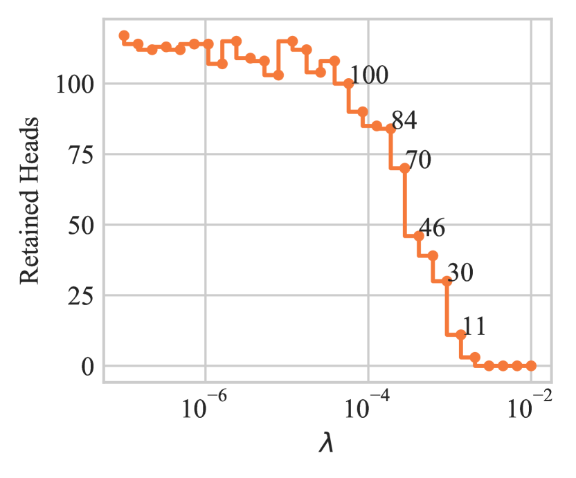
Figure 3: Number of unpruned heads as a function of $L_{0}$ regularization coefficient $\lambda$ for Voita et al..

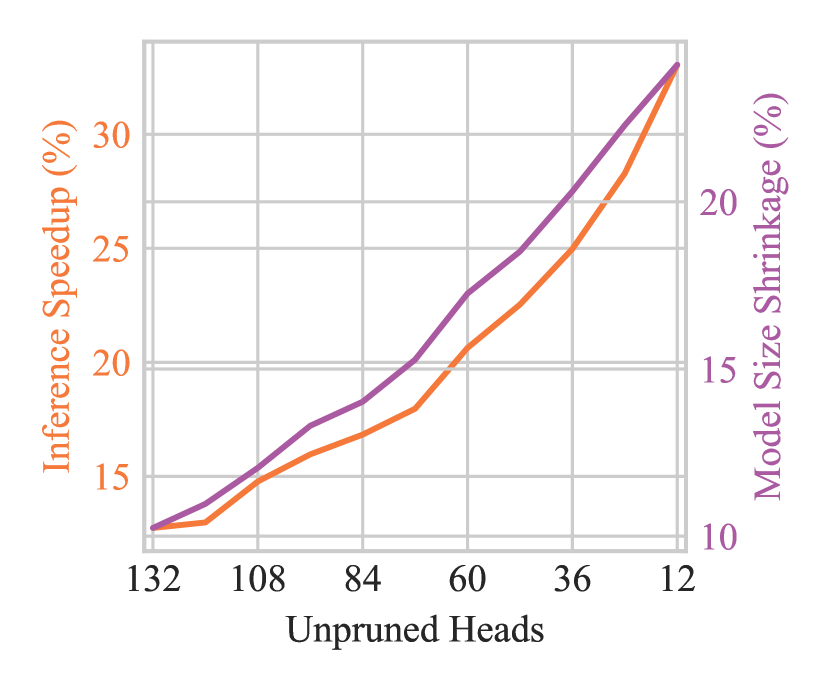
Figure 4: Inference speedup ($\%$) and model size shrinkage ($\%$) of pruned BERT model on the MNLI-mismatched validation set as a function of remaining heads.

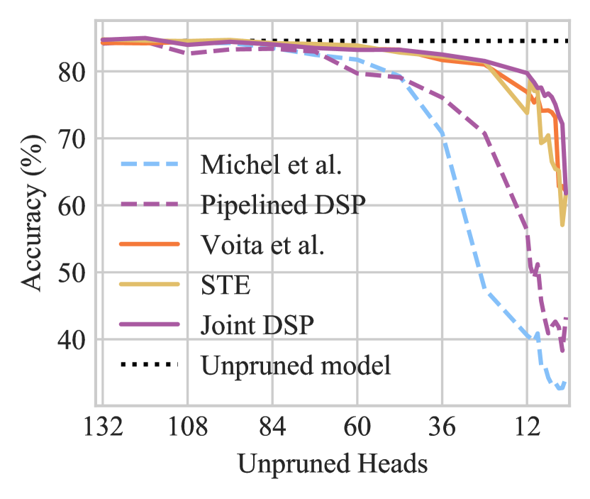
(a) Accuracy on the MNLI-mismatched validation set as a function of number of unpruned heads in BERT.

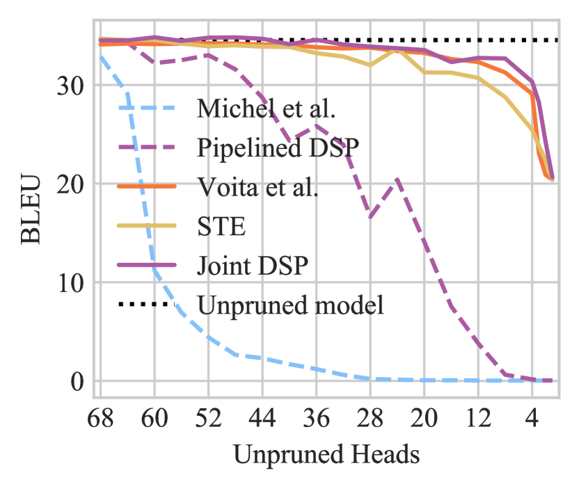
(b) BLEU score on IWSLT test set as a function of number of unpruned heads in Enc–Dec.

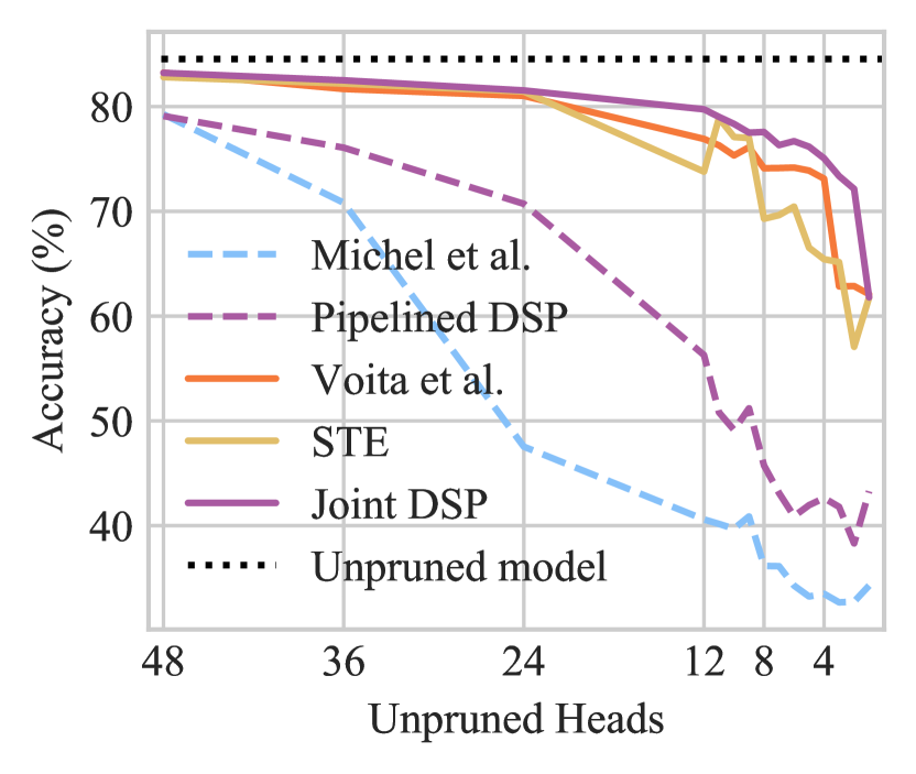
(c) We zoom in on the portion of Fig. 2(a) where few heads remain unrpuned.

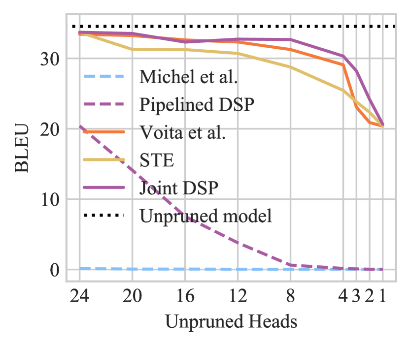
(d) We zoom in on the portion of Fig. 2(b) where few heads remain unrpuned.

Figure 2: A comparison of various pruning methods.

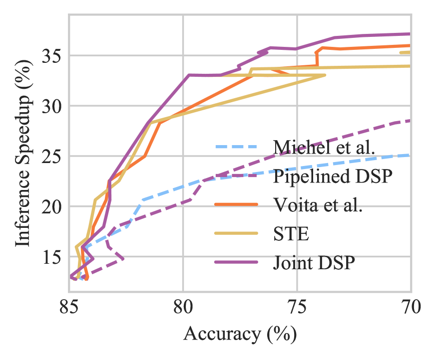
(a) Inference speedup as a function of accuracy.

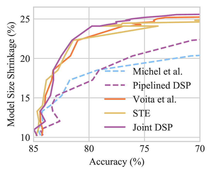
(b) Model size shrinkage as a function of accuracy.

Figure 5: Inference speedup ($\%$) and model size shrinkage ($\%$) of the various pruned BERT models vs. accuracy ($\%$) on the MNLI-mismatched validation set.

5 Discussion

5.1 Pipelined Pruning

We first compare the two pipelined pruning methods: Michel et al. (2019) and pipelined DSP. As shown in Fig. 2, pipelined DSP outperforms Michel et al. by a large margin. For example, on the MNLI task, when there are $24$ heads left in the model, pipelined DSP keeps an accuracy above $70\%$, but Michel et al. drops below $50\%$. On the IWSLT dataset, when only $24$ heads are left unpruned, the Enc–Dec pruned with Michel et al. cannot produce meaningful outputs ($\approx 0$ BLEU score), while pipelined DSP achieves higher than $20$ BLEU. The results indicate that the learned head importance scores are more useful for pruning than those computed with gradient-based measures.

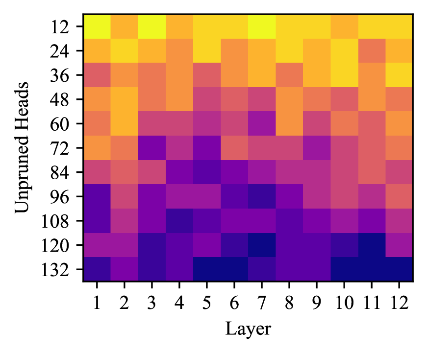
(a) BERT

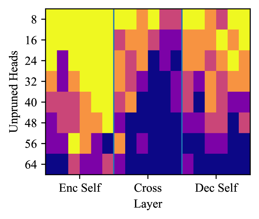
(b) Enc–Dec

Figure 6: Distribution of unpruned heads across layers. Darkness of the color increases monotonically with the number of heads.

5.2 Joint Pruning

We then compare the three joint pruning methods: Voita et al. (2019), STE and joint DSP. Impressively, joint DSP is able to prune up to $91.6\%$ (12 heads left) and $94.4\%$ (4 heads left) of heads in BERT and the Enc–Dec respectively without causing much degradation in test performance ($5.5\%$ drop in accuracy for MNLI and $4.22$ drop in BLEU score for IWSLT). Voita et al. and STE are neck and neck with joint DSP when the model is lightly pruned, but joint DSP gains the upper hand when less than $\nicefrac{{1}}{{6}}$ of the heads are left unpruned.

In addition, with Voita et al.’s method, it is much harder to enforce a hard constraint on the number of unpruned heads. This difficulty is intrinsic to their method as Voita et al.’s method relies on the regularization coefficient $\lambda$ to indirectly control the sparsity. In practice, our experiments indicate that $\lambda$ is hard to tune and there are certain levels of sparsity that cannot be reached. The difficulty in tuning $\lambda$ is shown in Fig. 3; we see that the number of unpruned heads does not decrease monotonically as $\lambda$ increases; on the contrary, it often fluctuates. There also appears to be an upper bound ($117$) on the number of heads that can be kept no matter how small $\lambda$ is. More importantly, a small increase in $\lambda$ can sometimes drastically reduce the number of heads. For instance, when $\lambda$ is increased from $0.0009$ to $0.0014$, the number of heads reduced quickly from $30$ to $11$. Therefore, we conclude that Voita et al.’s method is inadequate if the user requires a pre-specified number of Transformer heads. In contrast, DSP (as well as STE), our proposal, enables us to directly specify the number of heads we want to keep in accordance with our computation budget.

5.3 Pipelined Pruning vs Joint Pruning

Lastly, we offer a philosophical comparison of the two pruning paradigms. It is clear from Fig. 2 that the joint pruning methods are superior to pipelined pruning methods for both tasks, as models sparsified with the joint pruning schemes (joint DSP, STE and Voita et al.) perform better than those pruned with pipelined schemes (pipelined DSP and Michel et al.) under almost every sparsity level. This suggests that joint training is more effective in finding sparse subnetworks than pipelined pruning. Moreover, joint pruning is also more computationally efficient. In addition to the same number of epochs required by both paradigms for training/fine-tuning, pipelined pruning requires us to learn or estimate gradient-based head importance scores for one extra epoch. Even though joint pruning methods train $H$ more parameters during training/fine-tuning, $H$ is typically orders of magnitudes smaller than the total number of model parameters, so the additional computational overhead is negligible.

5.4 Inference Efficiency

In this section, we obtain the pruned model by actually removing the heads with mask values $0$. Empirically, we observe substantial wallclock improvements in our pruned models compared to unpruned models. In practice, we found that the inference efficiency improves monotonically as the number of unpruned heads decrease and is not significantly impacted by the distribution of heads across layers. Taking BERT on MNLI-mismatched validation set (batch size of 8) as an example, we randomly sample $10$ head masks for each sparsity level, measure their inference speedup and model size shrinkage compared to the unpruned model, and report the average in Fig. 4. In general, head pruning does lead to a faster and smaller model, and the more we prune, the faster and smaller the model becomes.

Comparison of various pruning schemes is displayed in Fig. 5. If we set a threshold for accuracy (e.g. 80%), joint DSP returns a model with a $\approx 33\%$ speedup in execution time and $\approx 24\%$ decrease in model size.

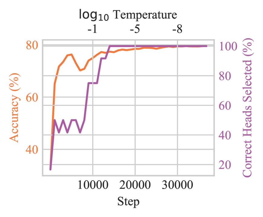
(a) With Annealing

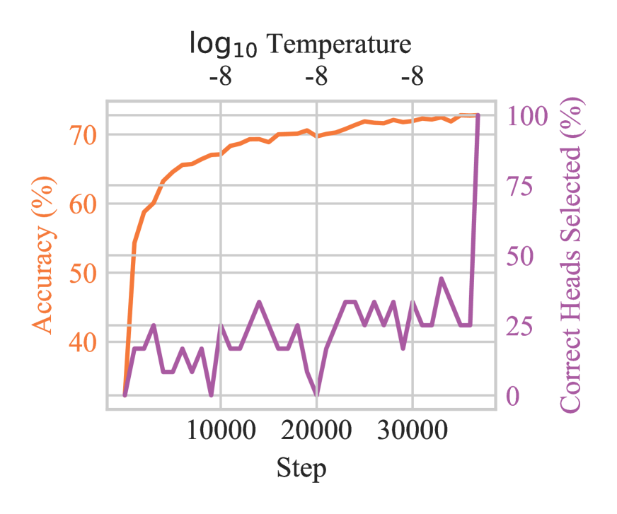
(b) Without Annealing

Figure 7: Training dynamics of joint DSP on BERT ($K=12$). The lower $x$-axis shows the number of training steps, and the upper $x$-axis shows the corresponding temperature in logarithm scale. Left $y$-axis (orange) shows test accuracy on MNLI-mismatched validation set. Right $y$-axis (purple) shows the percentage of heads selected at current step that are kept eventually.

5.5 Distribution of Heads

We visualize the distribution of unpruned heads across different layers in Fig. 6. For BERT (Fig. 6(a)), we observe that the top layers (10–12) are the first to be pruned and the heads in the middle layers (3–7) are mostly retained. This observation is in conformity with Prasanna et al. (2020); Sajjad et al. (2021). Budhraja et al. (2020) also highlights the importance of middle layers but finds no preference between top and bottom layers. For Enc–Dec (Fig. 6(b)), we find that a lot more encoder–decoder cross attention heads are retained compared to the other two types of attentions (encoder and decoder self attentions). The encoder self-attention heads are completely pruned away when less than $16$ heads are left, which again conforms with the observations of Michel et al. (2019) and Voita et al. (2019).

5.6 Analysis of Training Dynamics

To better understand our joint DSP approach, we inspect its behavior during training. We plot the intermediate accuracy of BERT during training when joint DSP ($K=12$) is applied in Fig. 7(a) (in orange). We also compute the percentage of heads selected at the current step that are eventually kept in the end (in purple). We observe the selected subset of heads is no longer updated after 14000 training steps (purple line stays at $100\%$). Therefore, the joint pruning process may be viewed as having two distinct phases—i) head selection and ii) fine-tuning. This piques one’s interest as it appears to superficially resemble a reversed pipelined pruning. During head selection, the subset of heads to be kept is determined and the model is adapted to the specified level of sparseness. During fine-tuning, the selected subnetwork is fine-tuned so that the testing accuracy improves steadily. Our experiments indicate that annealing is essential for training a high-performance pruner: It allows the model to gradually settle down on one particular subset of heads, whereas without annealing the pruner never converges to a fixed set and thereby does not enter the fine-tuning phase. See Fig. 7(b) for a visualization.

5.7 Summary

The five pruning methods discussed in this paper are summarized in Tab. 1. Joint DSP is able to maintain the highest test performance while consuming similar computational resources to Voita et al. and offering fine-grained control over the number of unpruned heads like Michel et al. It is worth noting that STE shares the same benefits of low computational overhead and exact sparsity control as joint DSP, despite being slightly inferior in performance. It also has less hyperparameters to tune and hence is easier to implement. Therefore, we believe STE could be favorable when test performance is not that critical.

6 Related Work

Unstructured Pruning.

Neural network pruning has been studied for decades. Early works include optimal brain damage LeCun et al. (1990) and optimal brain surgeon Hassibi et al. (1994), which approximate the loss function of a trained model with a second-order Taylor expansion and remove certain parameters in the network while minimizing impact on loss. Recent years have seen a resurgence in this approach Molchanov et al. (2017b); Theis et al. (2018); Michel et al. (2019). More recently, magnitude pruning that discards parameters with small absolute values has gained much popularity Han et al. (2015, 2016); Guo et al. (2016); Zhu and Gupta (2018). Gordon et al. (2020) applies magnitude pruning to BERT and shows that the model has similar prunability and transferability whether pruned after pre-training or after fine-tuning. Related to magnitude based pruning is movement pruning introduced by Sanh et al. (2020) which considers changes in weights instead of magnitudes for pruning.

Structured Pruning.

Different from above-mentioned unstructured pruning methods that prune individual parameters, structured pruning methods prune at a higher level, such as convolutional channels, attention heads, or even layers. Structured pruning almost always leads to a decrease in model size and inference cost, while unstructured pruning often results in sparse matrices, which cannot be utilized without dedicated hardware or libraries Han et al. (2016). Previously, structured pruning had primarily been applied to convolutional neural networks Wen et al. (2016); Li et al. (2017); Luo et al. (2017); He et al. (2017); Liu et al. (2017); Huang and Wang (2018), but it has recently been applied to NLP, in the form of layer pruning Fan et al. (2020); Sajjad et al. (2021) and head pruning Michel et al. (2019); Voita et al. (2019); McCarley et al. (2021) of Transformer-based models. Apart from compression and speedup, head pruning is also helpful for model analysis; Voita et al. (2019) finds that the heads that survive pruning play consistent and linguistically-interpretable roles. Prasanna et al. (2020) discovered the heads that are pruned last tend to be in the earlier and middle layers.

Methods	Computation Overhead	Sparsity Controllability	Test Performance
Michel et al.
Pipelined DSP (this paper)
Voita et al.
STE (this paper)
Joint DSP (this paper)

Table 1: Qualitative Comparison of Different Pruning Methods

Dropout for Pruning.

A variety of regularizers have been used to sparsify neural networks. For example, Han et al. (2015) applies $L_{1}$ regularization, and Louizos et al. (2018) applies $L_{0}$ regularization. Dropout, as one of the regularization methods, has also been demonstrated to be effective for converting a model to be robust to pruning. It was discovered that dropout encourages sparsity when dropout was proposed Srivastava et al. (2014). Recently, the assumption that the model trained with dropout tend to be more robust to post-hoc pruning was also explored. LayerDrop Fan et al. (2020) randomly drops entire layers in Transformer with a fixed dropout rate during training and simply keeps every other layer during inference. Targeted Dropout Gomez et al. (2019) ranks units in the order of magnitude and only applies dropout to those with small magnitudes and performs magnitude pruning afterwards. Molchanov et al. (2017a) introduces variational dropout, which allows learning a different dropout rate for each unit. Kingma et al. (2015) extends it for pruning by keeping only the units with lower dropout rate for test. Our approach is in the same vein but distinct as we learn importance variables rather than dropout rate and the number of heads to be dropped is specified explicitly, which allows us a control over sparsity.

Lottery Ticket Hypothesis.

Frankle and Carbin (2019) proposes the Lottery Ticket Hypothesis that there exist subnetworks ("winning lottery tickets") in a over-parameterized model, which can be trained in isolation to reach comparable test performance as the original network in a similar number of iterations. It shows such tickets can be discovered through magnitude pruning. Brix et al. (2020) successfully applies the hypothesis to the Transformer. Prasanna et al. (2020); Behnke and Heafield (2020) demonstrate head pruning may also be used to select a winning subnetwork.

7 Conclusion

We propose differentiable subset pruning, a novel method for sparsifying Transformers. The method allows the user to directly specify the desired sparsity level, and it achieves a better sparsity–accuracy trade-off compared to previous works, leading to a faster and more efficient model after pruning. It demonstrates improvements over existing methods for pruning two different models (BERT and Enc–Dec) on two different tasks (textual entailment and machine translation), respectively. It can be applied in both pruning paradigms (pipelined and joint pruning). Although we study head pruning in the paper, our approach can be extended to other structured and unstructured pruning scenarios. In future work, it would be interesting to look into such cases.

Appendix A Experimental Setup

We report the hyperparameters for joint DSP we use in our experiments in Tab. 2, which are obtained by tuning on the validation set.

	BERT	Enc–Dec
$\tau_{\text{ini}}$	$1000$	$0.1$
$\tau_{\text{end}}$	$1e-08$	$1e-08$
$N_{\text{cooldown}}$	$25000$	$15000$
lr for $w_{h}$	$0.5$	$0.2$

Table 2: Hyperparameters used for joint DSP.

Appendix B Analysis of Training Dynamics

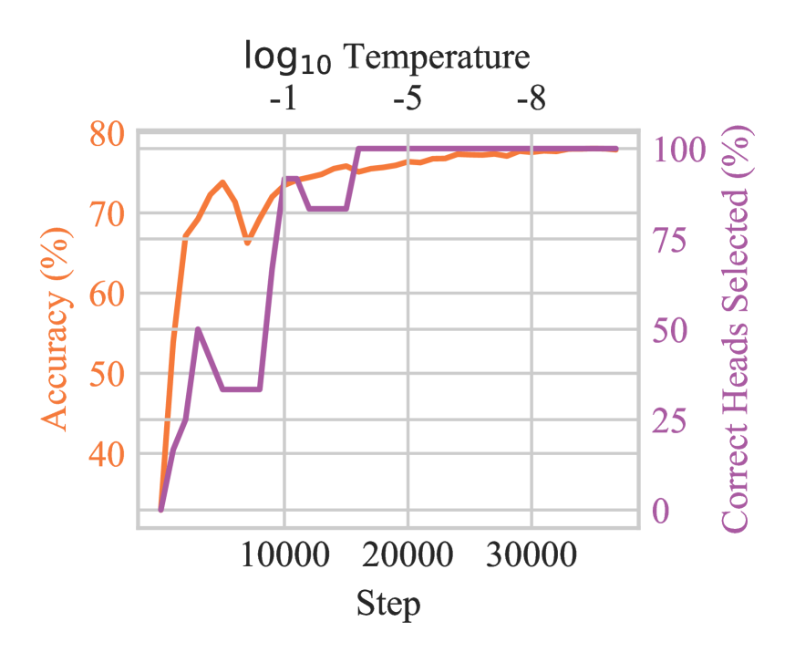
(a) $K=8$ with annealing

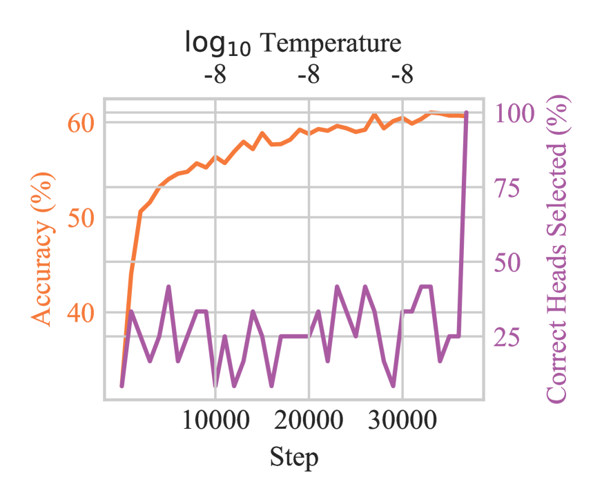
(b) $K=8$ without annealing

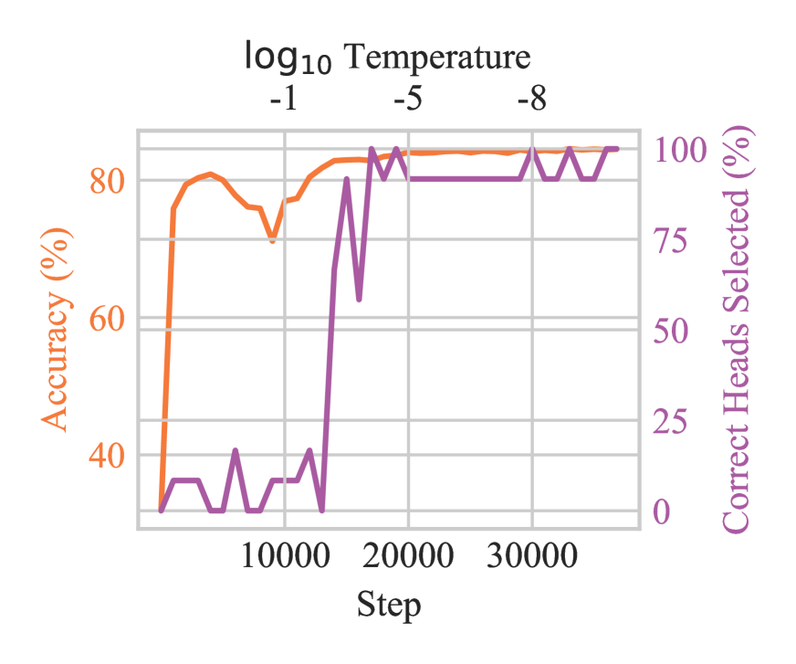
(c) $K=108$ with annealing

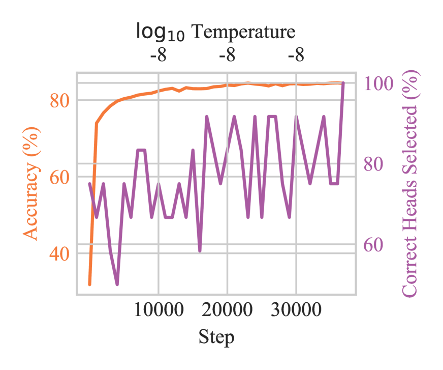
(d) $K=108$ without annealing

Figure 8: Training dynamics of joint DSP on BERT. The lower $x$-axis shows the number of training steps, and the upper $x$-axis shows the corresponding temperature in logarithm scale. Left $y$-axis (orange) shows test accuracy on MNLI-mismatched validation set. Right $y$-axis (purple) shows the percentage of heads selected at current step that are kept eventually.

We present two more examples where heads are scarce ($K=8$) or redundant ($K=108$). In Fig. 8(a), we observe the same two-phase training behavior as $K=12$. The selected subset of heads is not altered anymore after $16000$ steps. In Fig. 8(c), unlike the cases where heads are very few, the head masks are constantly updated throughout the training procedure. Yet a large portion ($91.7\%$) of the heads remain unchanged after $17000$ steps. Its two-phase behavior is still apparent in comparison with training without annealing (Fig. 8(d)).

Appendix C Detailed Results

The detailed results for plotting Fig. 2 are presented in Tab. 3.

Unpruned Heads	Michel et al.	Pipelined DSP	Voita et al.	STE	Joint DSP
132	84.38	84.15	84.26	84.77	84.70
120	84.60	84.41	84.18	84.59	84.97
108	84.19	82.64	84.39	84.52	83.95
96	84.24	83.27	84.42	84.68	84.41
84	83.50	83.37	84.00	84.20	84.02
72	82.47	82.95	83.93	84.08	83.48
60	81.74	79.69	83.37	83.85	83.21
48	79.26	79.10	83.24	82.81	83.22
36	70.82	76.08	81.68	82.20	82.51
24	47.54	70.72	81.02	81.44	81.54
12	40.59	56.29	76.91	73.79	79.74
11	40.16	50.81	76.30	78.91	79.02
10	39.71	49.14	75.34	77.10	78.35
9	40.88	51.20	76.12	76.99	77.51
8	36.16	45.74	74.12	69.29	77.57
7	36.13	43.11	74.14	69.64	76.32
6	34.28	40.90	74.18	70.45	76.70
5	33.24	41.95	73.89	66.53	76.17
4	33.49	42.64	73.12	65.43	75.06
3	32.68	41.79	62.84	65.15	73.36
2	32.74	38.30	62.87	57.07	72.14
1	34.28	43.28	62.09	61.79	61.79

(a) Accuracy on the MNLI-mismatched validation set as a function of number of remaining heads in BERT.

Unpruned Heads	Michel et al.	Pipelined DSP	Voita et al.	STE	Joint DSP
68	32.87	34.19	34.10	34.69	34.52
64	29.08	34.29	34.19	34.55	34.51
60	11.18	32.21	34.14	34.56	34.83
56	6.91	32.52	34.19	34.19	34.46
52	4.41	33.02	34.23	33.92	34.79
48	2.64	31.58	34.20	34.02	34.82
44	2.30	28.70	34.08	33.88	34.68
40	1.70	24.35	34.06	33.85	34.13
36	1.20	25.84	33.82	33.22	34.58
32	0.61	23.94	33.70	32.88	34.10
28	0.19	16.63	33.78	32.01	33.89
24	0.13	20.40	33.44	33.71	33.72
20	0.07	14.11	33.25	31.27	33.54
16	0.07	7.55	32.62	31.25	32.32
12	0.05	3.80	32.33	30.71	32.74
8	0.04	0.63	31.26	28.77	32.68
4	0.04	0.16	29.09	25.45	30.33
3	0.04	0.09	23.08	23.83	28.22
2	0.04	0.05	20.89	22.35	24.18
1	0.04	0.05	20.38	20.37	20.64

(b) BLEU score on IWSLT test set as a function of number of unpruned heads in Enc–Dec.

Table 3: A comparison of various pruning methods.

References

- Bahdanau et al. (2015) Dzmitry Bahdanau, Kyunghyun Cho, and Yoshua Bengio. 2015. Neural machine translation by jointly learning to align and translate. In 3rd International Conference on Learning Representations.
- Behnke and Heafield (2020) Maximiliana Behnke and Kenneth Heafield. 2020. Losing heads in the lottery: Pruning transformer attention in neural machine translation. In Proceedings of the 2020 Conference on Empirical Methods in Natural Language Processing (EMNLP), pages 2664–2674, Online. Association for Computational Linguistics.
- Bengio et al. (2013) Yoshua Bengio, Nicholas Léonard, and Aaron C. Courville. 2013. Estimating or propagating gradients through stochastic neurons for conditional computation. CoRR, abs/1308.3432v1.
- Brix et al. (2020) Christopher Brix, Parnia Bahar, and Hermann Ney. 2020. Successfully applying the stabilized lottery ticket hypothesis to the transformer architecture. In Proceedings of the 58th Annual Meeting of the Association for Computational Linguistics, pages 3909–3915, Online. Association for Computational Linguistics.
- Brown et al. (2020) Tom Brown, Benjamin Mann, Nick Ryder, Melanie Subbiah, Jared D. Kaplan, Prafulla Dhariwal, Arvind Neelakantan, Pranav Shyam, Girish Sastry, Amanda Askell, Sandhini Agarwal, Ariel Herbert-Voss, Gretchen Krueger, Tom Henighan, Rewon Child, Aditya Ramesh, Daniel Ziegler, Jeffrey Wu, Clemens Winter, Chris Hesse, Mark Chen, Eric Sigler, Mateusz Litwin, Scott Gray, Benjamin Chess, Jack Clark, Christopher Berner, Sam McCandlish, Alec Radford, Ilya Sutskever, and Dario Amodei. 2020. Language models are few-shot learners. In Advances in Neural Information Processing Systems, volume 33, pages 1877–1901.
- Budhraja et al. (2020) Aakriti Budhraja, Madhura Pande, Preksha Nema, Pratyush Kumar, and Mitesh M. Khapra. 2020. On the weak link between importance and prunability of attention heads. In Proceedings of the 2020 Conference on Empirical Methods in Natural Language Processing (EMNLP), pages 3230–3235, Online. Association for Computational Linguistics.
- Cettolo et al. (2014) Mauro Cettolo, Jan Niehues, Sebastian Stüker, Luisa Bentivogli, and Marcello Federico. 2014. Report on the 11 IWSLT evaluation campaign. In Proceedings of the International Workshop on Spoken Language Translation, Hanoi, Vietnam, volume 57.
- Clark et al. (2019) Kevin Clark, Urvashi Khandelwal, Omer Levy, and Christopher D. Manning. 2019. What does BERT look at? An analysis of BERT’s attention. In Proceedings of the 2019 ACL Workshop BlackboxNLP: Analyzing and Interpreting Neural Networks for NLP, pages 276–286.
- Cotterell and Eisner (2017) Ryan Cotterell and Jason Eisner. 2017. Probabilistic typology: Deep generative models of vowel inventories. In Proceedings of the 55th Annual Meeting of the Association for Computational Linguistics (Volume 1: Long Papers), pages 1182–1192, Vancouver, Canada. Association for Computational Linguistics.
- Devlin et al. (2019) Jacob Devlin, Ming-Wei Chang, Kenton Lee, and Kristina Toutanova. 2019. BERT: Pre-training of deep bidirectional transformers for language understanding. In Proceedings of the 2019 Conference of the North American Chapter of the Association for Computational Linguistics: Human Language Technologies, Volume 1 (Long and Short Papers), pages 4171–4186, Minneapolis, Minnesota. Association for Computational Linguistics.
- Ettinger (2020) Allyson Ettinger. 2020. What BERT is not: Lessons from a new suite of psycholinguistic diagnostics for language models. Transactions of the Association for Computational Linguistics, 8:34–48.
- Fan et al. (2020) Angela Fan, Edouard Grave, and Armand Joulin. 2020. Reducing transformer depth on demand with structured dropout. In 8th International Conference on Learning Representations.