Tests for the existence of horizon through gravitational waves from a small binary in the vicinity of a massive object

Abstract

In this letter we calculate the gravitational waves (GWs) emitted from a small binary (SB) by solving the Teukolsky equation in the background of a massive exotic compact object (ECO) which is phenomenologically described by a Schwarzschild geometry with a reflective boundary condition at its “would-be” horizon. The “continuous echo” waves propagating to infinity due to reflectivity of ECO at its “would-be” horizon provide an exquisite probe to the nature of the ECO’s horizon.

Introduction. Black holes are predicted by general relativity as the compact stellar remnants of gravitational collapse of massive stars. Detection of event horizon, marking the boundary within which future null infinity cannot be reached, is supposed to be the decisive evidence for black hole. Both the gravitational wave (GW) detections Abbott et al. (2016a, b, c, 2017) and the observations of supermassive black holes by the Event Horizon Telescope Akiyama et al. (2019a, b, c, d, e) provide the elegant avenues toward the physics near the event horizon of black hole. However, no experiment yet is able to reveal the geometry structure near event horizon although the black hole paradigm is consistent with hitherto all electromagnetic and GW observations Abbott et al. (2019, 2021); Akiyama et al. (2019a, b). In particular, Barausse and Cardoso et.al.Barausse et al. (2014); Cardoso et al. (2016a) argued that GW from a binary coalescence, especially the ringdown waveform, could not be regarded as a conclusive evidence for the existence of event horizon after the merger. Furthermore, event horizon plays a central role in the black hole information paradox Unruh and Wald (2017), and the behavior of event horizon is important to the theory of quantum gravity. Thus, probing the existence of event horizon is the cornerstone of strong-gravity research and become one of the frontier researches of fundamental physics.

On the other hand, the concept of horizonless object, namely exotic compact object (ECO), was put forward as an alternative to the classical black hole paradigm. ECO is motivated either by candidate theories of quantum gravity, including the ECO models of firewall, wormhole, fuzzball, and black holes modified by generalized uncertainty principle Mathur (2005, 2008); Almheiri et al. (2013); Giddings and Psaltis (2018); Bianchi et al. (2020); Bena and Mayerson (2020); Mukherjee and Chakraborty (2020); Buoninfante et al. (2020), or by the physics beyond standard model of particle physics, including ECO models of boson star and gravastar Mazur and Mottola (2001, 2004); Pani et al. (2009); Palenzuela et al. (2017). Despite different model of ECO, it may be phenomenologically described by a standard black hole with a reflective boundary condition given at its “would-be horizon”, i.e., its physical surface close to the event horizon predicted by general relativity, as a result of our beliefs that the difference between ECO and black hole would be only significant in the Planckian or near-Planckian scale near the event horizon Cardoso and Pani (2019a).

In literature there are several methodologies to test the nature of dark compact objects based on GW astronomy: (i) detecting the small corrections to the GW phase during binary inspiral stage, which is driven by different multipolar structures, tidal deformation, tidal heating, resonance excitation, and the correction of gravitational waves from extreme-mass-ratio inspiral systems Hughes (2013); Krishnendu et al. (2017); Cardoso et al. (2017); Maselli et al. (2018); Sennett et al. (2017); Krishnendu et al. (2019); Datta and Bose (2019); Datta et al. (2020); Dreyer et al. (2004); Berti et al. (2006, 2016); Berti and Cardoso (2006); Cardoso et al. (2019); Datta et al. (2020); Maggio et al. (2021a); Sago and Tanaka (2021); (ii) late-time echoes in the GW waveforms afterwards the merger stage, induced by the presence of structure close to the gravitational radius of the ECO Cardoso et al. (2016b, c); Cardoso and Pani (2017); Abedi et al. (2017); Conklin et al. (2018); Tsang et al. (2018); Lo et al. (2019); Nielsen et al. (2019); Uchikata et al. (2019); Tsang et al. (2020); Xin et al. (2021); (iii) stochastic GW background caused by ergoregion instability of ECOs Barausse et al. (2018); Fan and Chen (2018); Du and Chen (2018). See Cardoso and Pani (2019b); Maggio et al. (2021b) for some recent review.

In this letter, we propose a new method to test the existence of event horizon through GWs emitted by a small binary (SB) in the background of a massive ECO. The idea is sketched out in Fig. 1. Usually the Center of Galaxy harbors a supermassive black hole (SMBH) Ghez et al. (2009); Kormendy and Ho (2013); McConnell and Ma (2013), and SB could form in a close orbit to the SMBH due to abundant astrophysical phenomena (see, e.g., Antonini and Perets (2012); McKernan et al. (2014); Chen et al. (2019); Inayoshi et al. (2017); Chen and Han (2018); Tagawa et al. (2020); Peng and Chen (2021)) and even merger in the inner-most stable circular orbit (ISCO) of the SMBH Peng and Chen (2021). The orbital radius of SB is much smaller than the orbital radius of their center of mass revolving around the SMBH, and thus compose a stable hierarchical triple system, the so called “binary-EMRI” system Chen and Han (2018). The gravitational radiation in such system has been studied in large amount of contexts, the waveforms are characterized by many unique features Cisneros et al. (2015); Meiron et al. (2017); Randall and Xianyu (2019a); Wong et al. (2019); Torres-Orjuela et al. (2019, 2020); D’Orazio and Loeb (2020); Ezquiaga and Zumalacárregui (2020); Ezquiaga et al. (2021); Hoang et al. (2018); Randall and Xianyu (2019b); Fang et al. (2019); Fang and Huang (2020); Yu and Chen (2021); Cardoso et al. (2021a). If the centering object is a massive ECO rather a SMBH, GWs emitted by the SB will be reflected to infinity at the “would-be” horizon of ECO, resulting the “continuous echo” waves, and thus provides a new probe to the “would-be” horizon of the massive ECO.

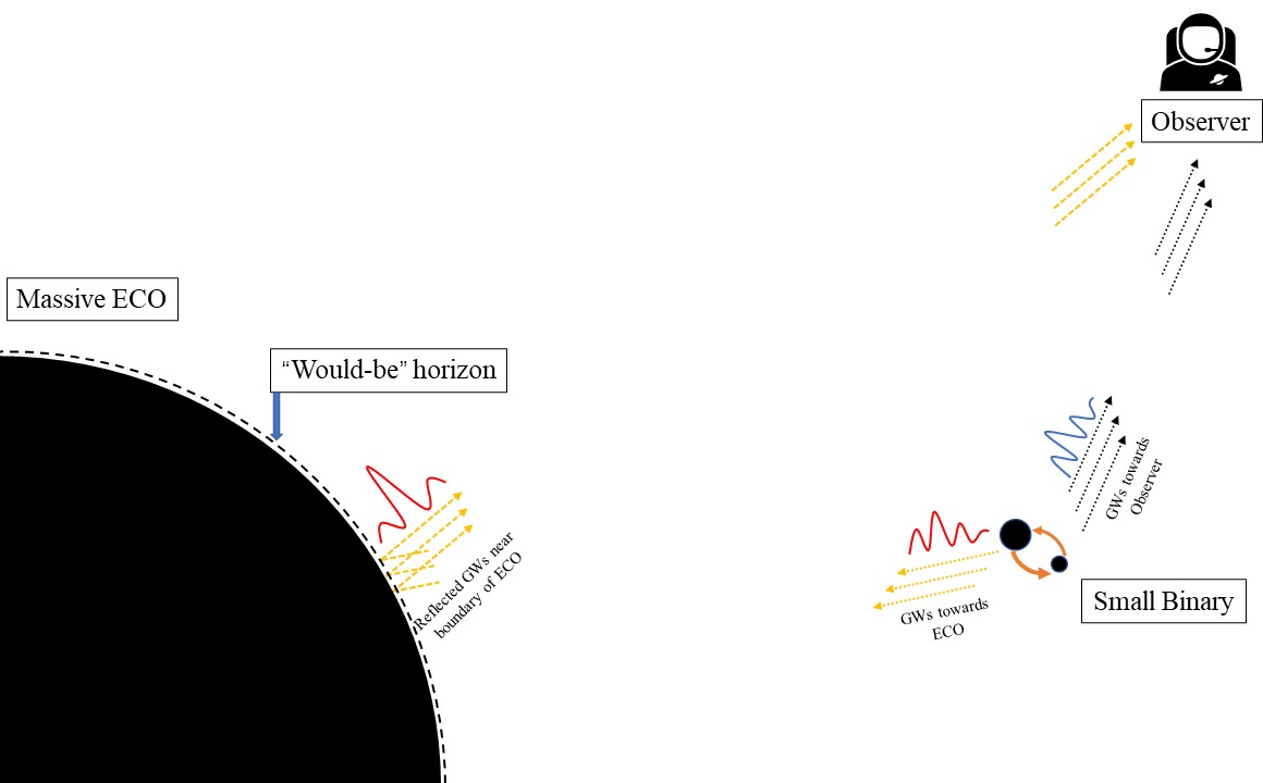
Figure 1: The illustration of the GWs of a small binary emitted in the ECO background detected by a distant observer.

Set up: the black hole perturbation theory. In this letter, we study the gravitational radiation of an SB in the background of a massive ECO. We focus on the non-spinning ECO, and then the external space-time geometry is described by the Schwarzschild metric except imposing a reflective boundary condition at the “would-be” horizon. The gravitational radiation of SB in such space-time can be obtained by solving the Teukolsky equation Teukolsky (1973) in the standard procedure.

For the usual perturbed Schwardzschild black hole (BH), the out-going gravitational radiation is governed by

$${}_{s}\mathcal{O}\ r^{4}\psi_{4}=4\pi r^{2}\hat{T},$$ (1)

where $\psi_{4}$ is the Newman-Penrose scalar describing the gravitational radiation at infinity, and the operator ${}_{s}\mathcal{O}$ under Schwarzschild geometry takes the form

$${}_{s}\mathcal{O} = -\left(\frac{r^{4}}{\Delta}\right)\partial_{t}^{2}+\left(\frac{1}{\sin^{2}\theta}\right)\partial_{\varphi}^{2}+\Delta^{-s}\partial_{r}\left(\Delta^{s+1}\partial_{r}\right)$$ (2)

$$+ \frac{1}{\sin\theta}\partial_{\theta}\left(\sin\theta\partial_{\theta}\right)+2s\left(\frac{i\cos\theta}{\sin^{2}\theta}\right)\partial_{\varphi}$$

$$+ 2s\left(\frac{Mr^{2}}{\Delta}-r\right)\partial_{t}-s\left(s\cot^{2}\theta-1\right)\,,$$

where $M$ is the mass of SMBH, $\Delta=r^{2}-2Mr$, and $s=-2$. Eq. (1) can be solved by decomposing $\psi_{4}$ and the source term $\hat{T}$ into

$$r^{4}\psi_{4}=\int d\omega\sum_{\ell m}e^{-i\omega t}{}_{-2}Y_{\ell m}(\theta,\varphi)R_{\omega\ell m}(r)\,,$$ (3)

$$4\pi r^{2}\hat{T}=\int d\omega\sum_{\ell m}e^{-i\omega t}{}_{-2}Y_{\ell m}(\theta,\varphi)T_{\ell m\omega}(r)\,,$$ (4)

where $\ {}_{-2}Y_{\ell m}$ is the spherical harmonics of spin weight $-2$. Then, Eq. (1) is reduced to an ordinary differential equation, namely the Teukolsky radial equation, as follows:

$$\!\left[r^{2}f\frac{d^{2}}{dr^{2}}-2(r-M)\frac{d}{dr}+U(r)\right]R_{\omega\ell m}(r)=T_{\omega\ell m},$$ (5)

where $f(r)=1-2M/r$, the potential $U(r)$ is given by

$$U(r)=f^{-1}\left[(\omega r)^{2}-4i\omega(r-3M)\right]-(\ell-1)(\ell+2)\,.$$ (6)

Teukolsky radial equation can be solved by the Green function method with standard procedure. Firstly, we need two linearly independent homogeneous solutions which satisfy proper boundary conditions. For a massive BH, the two homogeneous functions are denoted by $R_{\omega\ell m}^{\text{H}}$ and $R_{\omega\ell m}^{\infty}$ satisfying the following pure in-going condition at the event horizon and pure out-going condition at spatial infinity

$$\begin{array}[]{l}R_{\omega\ell m}^{\text{H}}\sim\left\{\begin{array}[]{ll}B_{\omega\ell m}^{\text{hole}}\Delta^{2}e^{-i\omega r_{*}}&r\rightarrow 2M\\ r^{3}B_{\omega\ell m}^{\text{out}}e^{i\omega r_{*}}+r^{-1}B_{\omega\ell m}^{\text{in}}e^{-i\omega r_{*}}&r\rightarrow+\infty\end{array}\right.\\ R_{\ell m\omega}^{\infty}\sim\left\{\begin{array}[]{ll}D_{\ell m\omega}^{\text{out}}e^{i\omega r_{*}}+\Delta^{2}D_{\ell m\omega}^{\text{in}}e^{-i\omega r_{*}}&r\rightarrow 2M\\ D_{\omega\ell m}^{\infty}r^{3}e^{i\omega r_{*}}&r\rightarrow+\infty\end{array}\right.\end{array}$$ (7)

where $r_{*}$ is the tortoise coordinate given by $r^{*}=r+2M\ln\left|\frac{r}{2M}-1\right|$. The Wronskian of Eq. (5) can be obtained from the asymptotic behavior at spatial infinity in Eq. (7), namely

$$\lim_{r\to\infty}{R^{\text{H}}_{\omega\ell m}R^{\infty\prime}_{\omega\ell m}-R^{\text{H}\prime}_{\omega\ell m}R^{\infty}_{\omega\ell m}\over r^{2}f(r)}=2i\omega B^{\text{in}}_{\omega\ell m}D^{\infty}_{\omega\ell m}\,,$$ (8)

where the prime denotes the derivative with respect to $r$. Therefore, the Green function $G^{\text{BH}}(r,r^{\prime})$ in BH case could be constructed by

$$G^{\text{BH}}\left(r,r^{\prime}\right)=\frac{1}{2i\omega B_{\omega\ell m}^{\text{in}}D^{\infty}_{\omega\ell m}}\times$$ (9)

$$\left[{\theta\left(r-r^{\prime}\right)\frac{R_{\omega\ell m}^{\text{H}}\left(r^{\prime}\right)R_{\omega\ell m}^{\infty}(r)}{r^{\prime 4}f^{2}(r^{\prime})}+\theta\left(r^{\prime}-r\right)\frac{R_{\omega\ell m}^{\text{H}}(r)R_{\omega\ell m}^{\infty}\left(r^{\prime}\right)}{r^{\prime 4}f^{2}(r^{\prime})}}\right]\,,$$

where $\theta\left(r-r^{\prime}\right)$ is the Heaviside step function, and the radial function $R_{\omega\ell m}$ at spatial infinity reads

$$R^{\text{BH}}_{\omega\ell m}(r) = \int_{2M}^{\infty}dr^{\prime}{G^{\text{BH}}(r,r^{\prime})T_{\omega\ell m}(r^{\prime})}$$ (10)

$$= {R^{\infty}_{\omega\ell m}(r)\over 2i\omega B^{\text{in}}_{\omega\ell m}D^{\infty}_{\omega\ell m}}\int_{2M}^{\infty}dr^{\prime}{R^{\text{H}}_{\omega\ell m}(r^{\prime})T_{\omega\ell m}(r^{\prime})\over r^{\prime 4}f^{2}(r^{\prime})}\,.$$

In order to get the homogenous solution $R_{\omega\ell m}(r)$, we usually solve the so-called Regge-Wheeler equation which has a form of wave equation as follows:

$$\left(\frac{d^{2}}{dr^{*2}}+\omega^{2}-V(r)\right)X_{\omega\ell m}(r)=0\,,$$ (11)

where

$$V(r)=\left(1-\frac{2M}{r}\right)\left(\frac{\ell(\ell+1)}{r^{2}}-\frac{6M}{r^{3}}\right)\,,$$ (12)

and $R_{\omega\ell m}(r)$ is related to $X_{\omega\ell m}(r)$ by the Chandrasekhar transformation Chandrasekhar (1993):

$$R_{\omega\ell m}(r) = r^{3}\left[\frac{2}{r}\left(1-\frac{3M}{r}\right)+2i\omega\right]\left[\frac{d}{dr_{*}}+i\omega\right]X_{\omega\ell m}(r)$$ (13)

$$+ r^{3}V(r)X_{\omega\ell m}(r).$$

The asymptotic behaviors of the Regge-Wheeler function $X_{\omega\ell m}(r)$ is then inherited from Eq. (7) as

$$\begin{array}[]{l}X_{\omega\ell m}^{H}\sim\left\{\begin{array}[]{ll}e^{-i\omega r_{*}}&r\rightarrow 2M\\ A_{\omega\ell m}^{\text{out}}e^{i\omega r_{*}}+A_{\omega\ell m}^{\text{in}}e^{-i\omega r_{*}}&r\rightarrow+\infty\end{array}\right.\\ X_{\ell m\omega}^{\infty}\sim\left\{\begin{array}[]{ll}C_{\ell m\omega}^{\text{out}}e^{i\omega r_{*}}+C_{\ell m\omega}^{\text{in}}e^{-i\omega r_{*}}&r\rightarrow 2M\\ e^{i\omega r_{*}}&r\rightarrow+\infty\end{array}\right.\end{array}$$ (14)

where $A^{\text{in}}_{\omega\ell m}$ is related to $B^{\text{in}}_{\omega\ell m}$ by

$$B^{\text{in}}_{\omega\ell m}={\left[12iM\omega-(l-1)l(l+1)(l+2)\right]\over 4\omega^{2}}A^{\text{in}}_{\omega\ell m}.$$ (15)

From now on, we switch to the gravitational radiation of an SB in the massive ECO background. The difference between ECO and BH is phenomenologically described by the reflective boundary condition at the “would-be” horizon of ECO which can be well-defined in the Regge-Wheeler equation due to its standard form of wave equation. The boundary conditions of the homogeneous Regge-Wheeler functions for ECO take the form

$$X_{\omega\ell m}^{\text{H ECO}} \sim e^{-i\omega r_{*}}+\mathcal{R}^{\text{ECO}}_{\omega\ell m}e^{i\omega r_{*}}\ \ \ \ for\ r\rightarrow 2M\,,$$

$$X_{\ell m\omega}^{\infty\ \text{ECO}} \sim e^{i\omega r_{*}}\ \ \ \ for\ r\rightarrow+\infty\,,$$ (16)

where $\mathcal{R}^{\text{ECO}}_{\omega\ell m}$ is the reflectivity which equals to zero for BH. Since the boundary condition for $X_{\omega\ell m}^{\infty\ \text{ ECO}}$ is the same as that for BH, we have $X_{\omega\ell m}^{\infty\ \text{ ECO}}=X_{\omega\ell m}^{{\infty}}$.

Similar to Eq. (9), the Green function of Teukolsky radial equation for ECO can be constructed with the homogeneous functions $R^{\text{H ECO}}_{\omega\ell m}$ and $R^{\infty}_{\omega\ell m}$, and $R^{\text{H ECO}}_{\omega\ell m}$ is related to $X_{\omega\ell m}^{\text{H ECO}}$ by the Chandrasekhar transformations as well. Since both $R^{\text{H ECO}}_{\omega\ell m}$ and $R^{\text{H}/\infty}_{\omega\ell m}$ satisfy with the homogeneous Teukolsky equation, the homogeneous function $R^{\text{H ECO}}_{\omega\ell m}$ can be taken as a linear superposition of $R^{\text{H}}_{\omega\ell m}$ and $R^{\infty}_{\omega\ell m}$

$$R^{\text{H ECO}}_{\omega\ell m}=R^{\text{H}}_{\omega\ell m}+\mathcal{K}R^{\infty}_{\omega\ell m}\,.$$ (17)

Consequently, the homogeneous Regge-Wheeler function $X^{\text{H ECO}}_{\omega\ell m}=X^{\text{H}}_{\omega\ell m}+\mathcal{K}X^{\infty}_{\omega\ell m}$. By demanding that $X^{\text{H ECO}}_{\omega\ell m}$ satisfies the boundary condition at the ECO “would-be” horizon in Eq. (Tests for the existence of horizon through gravitational waves from a small binary in the vicinity of a massive object), the coefficient $\mathcal{K}$ is given by Mark et al. (2017)

$$\mathcal{K}=\dfrac{\mathcal{R}^{\text{ECO}}_{\omega\ell m}\mathcal{T}^{\text{BH}}_{\omega\ell m}}{1-\mathcal{R}^{\text{ECO}}_{\omega\ell m}\mathcal{R}^{\text{BH}}_{\omega\ell m}}\,,$$ (18)

where $\mathcal{R}^{\text{BH}}_{\omega\ell m}$ and $\mathcal{T}^{\text{BH}}_{\omega\ell m}$ are the reflection and transmission amplitude of the BH potential barrier, namely

$$\mathcal{T}^{\text{BH}}_{\omega\ell m}=\dfrac{1}{C^{\text{out}}_{\omega\ell m}};\quad\mathcal{R}^{\text{BH}}_{\omega\ell m}=\dfrac{C^{\text{in}}_{\omega\ell m}}{C^{\text{out}}_{\omega\ell m}}.$$ (19)

Thus, the Green function for ECO, $G^{\text{ECO}}(r,r^{\prime})$, reads

$$G^{\text{ECO}}(r,r^{\prime})=G^{\text{BH}}(r,r^{\prime})+G^{\text{DEF}}(r,r^{\prime}),$$ (20)

where

$$G^{\text{DEF}}(r,r^{\prime})=\dfrac{\mathcal{K}}{2i\omega B^{\text{in}}_{\omega\ell m}D^{\infty}_{\omega\ell m}}\dfrac{R_{\omega\ell m}^{\mathrm{\infty}}(r)R_{\omega\ell m}^{\mathrm{\infty}}\left(r^{\prime}\right)}{r^{\prime 4}f^{2}(r^{\prime})}.$$ (21)

Since the Green function in Eq. (20) is separated into the BH part and the part related to the ECO reflectivity, the radial function of the GW emitted by the SB is also separated into

$$R_{\omega\ell m}^{\text{ECO}}(r)=R_{\omega\ell m}^{\text{BH}}(r)+R_{\omega\ell m}^{\mathrm{DEF}}(r)\,,$$ (22)

where

$$R^{\text{DEF}}_{\omega\ell m}(r) \!=\! \int_{2M}^{\infty}dr^{\prime}{G^{\text{DEF}}(r,r^{\prime})T_{\omega\ell m}(r^{\prime})}$$ (23)

$$= \dfrac{\mathcal{R}^{\text{ECO}}_{\omega\ell m}\mathcal{R}^{\text{BH}}_{\omega\ell m}}{1-\mathcal{R}^{\text{ECO}}_{\omega\ell m}\mathcal{R}^{\text{BH}}_{\omega\ell m}}R^{\text{eff}}(r)\,,$$

with $R^{\text{eff}}(r)$ given by

$$R^{\text{eff}}(r)\!=\!\dfrac{R_{\omega\ell m}^{{\infty}}(r)/C^{\text{in}}_{\omega\ell m}}{2i\omega B^{\text{in}}_{\omega\ell m}D^{\infty}_{\omega\ell m}}\!\int_{2M}^{\infty}\!dr^{\prime}{R_{\omega\ell m}^{{\infty}}(r^{\prime})T_{\omega\ell m}(r^{\prime})\over r^{\prime 4}f^{2}(r^{\prime})}.$$ (24)

The function $R^{\text{DEF}}_{\omega\ell m}(r)$ describes the waveform being reflected by the “would-be” horizon of ECO. Here, $R^{\text{DEF}}_{\omega\ell m}(r)$ can be re-written by the geometric series of $\mathcal{R}^{\text{ECO}}_{\omega\ell m}\mathcal{R}^{\text{BH}}_{\omega\ell m}$ (which is smaller than unity). In this sense, $R^{\text{DEF}}_{\omega\ell m}(r)$ can be physically explained as the linear superposition of repeated $R^{\text{eff}}(r)$ with the coefficient $(\mathcal{R}^{\text{ECO}}_{\omega\ell m}\mathcal{R}^{\text{BH}}_{\omega\ell m})^{n}$, which leads to the phenomenon called “echo”, similar to that after the ringdown signal of a merger event discussed in Mark et al. (2017). Therefore, the GWs detected by a distant observer include both the waveforms emitted by the SB in the BH background and the “echo” waves reflected by the “would-be” horizon of ECO. This is just what is illustrated in Fig. 1.

Setting sources. We model the SB as two point particles of mass $m_{1}$ and $m_{2}$, whose energy momentum tensor is given by

$$T^{\mu\nu}(x)= m_{1}\int_{-\infty}^{\infty}\delta^{(4)}(x-z(\tau_{1})){dz^{\mu}(\tau_{1})\over d\tau_{1}}{dz^{\nu}(\tau_{1})\over d\tau_{1}}d\tau_{1}$$ (25)

$$+(1\to 2),$$

where $z_{i}^{\mu}=(t(\tau_{i}),r(\tau_{i}),\theta(\tau_{i}),\varphi(\tau_{i}))$ (with $i=1,2$) are the world lines of the two point particles in the SB, and the normalization condition is given by $\int\delta^{(4)}(x)\sqrt{-g}d^{4}x=1$. For simplicity, we consider these two point particles have the same mass $m_{1}=m_{2}=\mu$. We take the orbital plane for the center of mass (CM) of SB as equatorial plane. For the two point particles of SB in the $\theta,\varphi$ plane, their positions are

$$\varphi_{1} = \Omega_{\text{CM}}t+\epsilon_{\varphi}\sin(\omega_{0}t),\varphi_{2}=\Omega_{\text{CM}}t-\epsilon_{\varphi}\sin(\omega_{0}t),$$

$$\theta_{1} = \pi/2+\epsilon_{\theta}\cos(\omega_{0}t),\theta_{2}=\pi/2-\epsilon_{\theta}\cos(\omega_{0}t),$$ (26)

where $\epsilon_{\varphi}=\delta R_{\varphi}/R$ and $\epsilon_{\theta}=\delta R_{\theta}/R$, $R$ is the circular orbital radius of CM, $\delta R_{\varphi}$ and $\delta R_{\theta}$ are the separations of the two point particles from their CM alone $\varphi$ and $\theta$ directions defined in the Schwarzschild coordinates. Thus $\epsilon_{\varphi}$ and $\epsilon_{\theta}$ characterize the orbit of the SB. And $\Omega_{\text{CM}}$ and $\omega_{0}$ in Eq. (Tests for the existence of horizon through gravitational waves from a small binary in the vicinity of a massive object) are the angular velocities of CM and SB in the coordinate frame. The coordinate frequency $\omega_{0}$ is related to the SB proper oscillation frequency $\omega^{\prime}_{0}$ by $\omega^{\prime}_{0}=U^{t}_{\text{CM}}\omega_{0}$, where $U^{t}_{\text{CM}}=(1-3M/R)^{-1/2}$ is time-component of the CM four velocity. In the rest frame of the SB, the proper quantity $\delta R^{\prime}_{\varphi}\propto 1/(\omega^{\prime}_{0})^{2/3}$ is rescaled by $\delta R^{\prime}_{\varphi}={\delta R_{\varphi}/(1-{2M\over r})}$. We could simply set $\epsilon_{\theta}\gg\epsilon_{\varphi}$, or $\epsilon_{\varphi}=0$ to resemble an elliptic orbit of the SB with a large eccentricity induced by the Kozai-Lidov mechanism M.L.Lidov (1962); Kozai (1962), and since $\epsilon_{\theta}\ll 1$, we could expand the source term by $\epsilon_{\theta}$ and keep to the lowest order. A similar set up could be seen in Cardoso et al. (2021a, b).

The waveforms in different ECO models. First of all, in order to sketch out the main feature of the GW waveform reflected by the “would-be” horizon of ECO, we consider a toy model in which the reflectivity is given by

$$\mathcal{R}_{\ell m\omega}=\epsilon\ e^{-2ib_{*}\omega},$$ (27)

where $r_{*}=b_{*}$ parameterizes the position of the physical surface, and the quantity $\epsilon\in(0,1)$ parameterizes the amplitude of reflectivity at the ECO surface. This toy model has a constant reflectivity for different frequencies.

In Fig. 2, we show the GW waveform of the SB emitted in the ECO background for an ECO under this model. The waveform is seen by a distant observer who is setting in the $\theta=\pi/2$ plane. From the upper panel of Fig. 2, we see that the GW amplitude of the SB is magnified due to the lensing of the massive body when the SB is moving close to the back of the massive BH/ECO. Compared to the GW emitted by the SB in the BH background, the GW of the SB emitted in the ECO background is enhanced due to the reflection of GWs at the ECO “would-be” horizon. The relative difference of the waveforms in the ECO and BH background become more obvious when the SB is not moving close to the back of the massive body, where no lensing magnification of the amplitude happens while the magnification of the GW amplitude due to the ECO reflectivity dominants. From the Middle and Lower panels of Fig. 2, we see that there are continuous GWs been reflected by the ECO surface, here, we call it “continuous echo” waves, which has a comparable magnitude with the GWs of the SB emitting in a BH background. And since the two echo waves in the middle and lower panels of Fig. 2 are only different by $b_{*}$ which characteristics the echo time delay (by $2b_{*}$), the only difference of the two echo waveforms is a shifting of a phase of $\Delta t=2b_{*}=60\text{M}$.

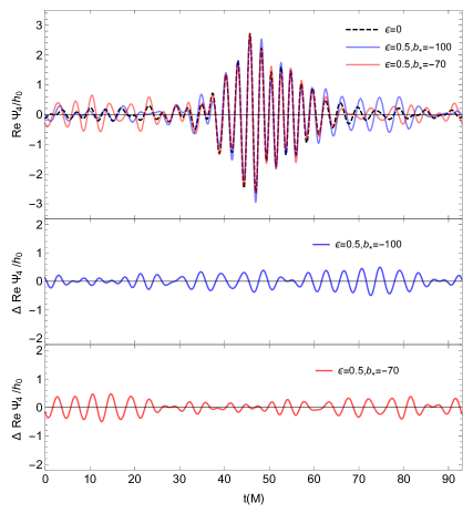
Figure 2: Upper panel: the waveform $\psi_{4}$ of the SB around a massive ECO with a constant reflectivity at the surface, observed by a distant observer whose eye sight is edge on with respect to the orbital plane of the CM of the SB, i. e., the plane of $\theta=\pi/2$. The GW polarizations are related to $\psi_{4}$ by $\psi_{4}=\frac{1}{2}\left(\ddot{h}_{+}-i\ddot{h}_{\times}\right)$. The CM of the SB is set in the inner-most stable circular (ISCO) of the ECO (orbital period is $93\text{M}$), and the SB orbit has a proper frequency of $\omega^{\prime}_{0}=1/\text{M}$. The black dashed line with $\epsilon=0$ corresponds to the BH case. Here, the amplitude of the waveform is rescaled by $h_{0}={\frac{L}{\mu^{2}}\frac{\mu^{1/3}}{(2\pi\omega^{\prime}_{0})^{2/3}}}$, where $L$ is the source distance to the observer. Middle and Lower panels: the difference of the SB waveforms in the ECO cases from that of the BH case, i.e. the “echo” waveforms due to the reflection of the ECO “would-be” horizon.

For a frequency-dependent reflectivity, such as Lorentzian reflectivity, it has a frequency dependence as follows

$$\mathcal{R}^{L}_{\ell m\omega}=\epsilon\left(\frac{i\Gamma}{\omega+i\Gamma}\right)e^{-2ib_{*}\omega}\,,$$ (28)

where the quantity $\Gamma$ characterizes a relaxation rate of the ECO surface and imposes a low-pass filtering of waves upon reflection in the frequency domain. For a distant observer, GWs with frequencies $|\omega|\lesssim\Gamma$ have the highest reflectivity. The GW waveform of the SB emitted in the ECO background with a Lorentzian reflectivity at the ECO “would-be” horizon is shown in Fig. 3. From Fig. 3, we can see that the amplitude of the reflected waves in the Lorentzian reflectivity case is smaller than that in the constant case for the same $\epsilon$. The reason is that all the GWs of different frequencies are equally reflected by the constant reflectivity, while in the Lorentzian case only the GWs with frequency $|\omega|<{\Gamma}$ are efficiently reflected.

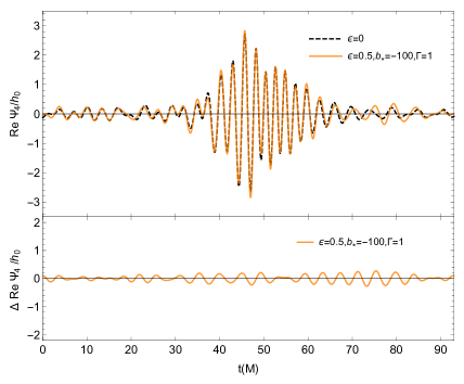
Figure 3: Upper panel: the edge on waveform of ECO with Lorentzian reflectivity at the ECO surface, and the orbital parameters are the same as those in Fig. 2. Lower panels: the “echo” waveforms due to the Lorentzian reflectivity at the ECO “would-be” horizon.

Detectability of the continuous echo. The GWs emitted by SB studied in this letter could be either LISA or LIGO-Virgo sources when they are moving during inspiral or late inspiral-merger-ringdown phase respectively, and the “continuous echo” waves could be detectable as well. For example, we consider $\omega^{\prime}_{0}=1/M$, and the GW frequency of SB is typically in LISA band. The detectability of the “continuous echo” waves can be revealed by comparing the GWs of the SB emitted in an ECO background with those in a black hole background. We denote the former waveform as $h_{1}$, and the later waveform as $h_{2}$. LISA employs a method called the “matched filtering” to discern the difference between two waveforms (Finn, 1992; Lindblom et al., 2008). The inner product of these two waveforms is defined by

$$\langle h_{1}|h_{2}\rangle=2\int_{0}^{\infty}{{\tilde{h}^{*}_{1}(f)\tilde{h}_{2}(f)+\tilde{h}_{1}(f)\tilde{h}^{*}_{2}(f)}\over S_{h}(f)}df,$$ (29)

where $S_{h}(f)$ is the spectral noise density Robson et al. (2019) and $\tilde{h}_{i}(f)$ denotes the Fourier transformation

$$\tilde{h}(f)=\int_{-\infty}^{\infty}e^{2\pi ift}h(t)dt.$$ (30)

These two waveforms are distinguishable if the condition

$$\langle\delta h|\delta h\rangle=\langle h_{1}-h_{2}|h_{1}-h_{2}\rangle>1$$ (31)

is satisfied. Or equivalently, the difference between these two waveforms can be described by the “fitting factor” (FF) (Apostolatos et al., 1994; Lindblom et al., 2008), namely

$$\textnormal{FF}={\langle h_{1}|h_{2}\rangle\over\sqrt{\langle h_{1}|h_{1}\rangle\langle h_{2}|h_{2}\rangle}},$$ (32)

and then one can compare it with a threshold FFS defined by

$$\textnormal{FFS}=1-{1\over\langle h_{1}|h_{1}\rangle+\langle h_{2}|h_{2}\rangle}.$$ (33)

Here FFS is closely related to the signal-to-noise ratio (${\rm SNR}=\sqrt{\langle h|h\rangle}$). If $h_{1}\simeq h_{2}$, we have $\textnormal{FFS}\simeq 1-1/(2\,{\rm SNR}^{2})$, and the criterion given in Eq. (31) is equivalent to $\textnormal{FF}<\textnormal{FFS}$. A signal with ${\rm SNR}\geq 10$, or equivaliently $\textnormal{FFS}\geq 0.995$, is needed for claiming a detection by LISA. Therefore a conservative estimation for a distinguishable continuous echo requires $\textnormal{FF}<0.995$. The fitting factor $(\textnormal{FF})$ vs. the reflective amplitude $\epsilon$ in the model with a constant reflectivity at the ECO surface is illustrated in Fig. 4 which indicates that the continuous echo is detectable as long as $\epsilon>0.17$.

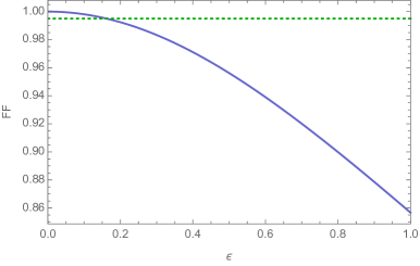
Figure 4: The fitting factor $(\textnormal{FF})$ vs. the reflective amplitude $\epsilon$ in the model with a constant reflectivity at the ECO surface. The green dashed line corresponds to $\textnormal{FF}=0.995$ which is a conservative threshold for detecting the continuous echo. Here, the mass of centering massive body is $10^{7}M_{\odot}$ and the total mass of the binary is $40M_{\odot}$.

Summary. The SBs could form in the vicinity of a supermassive compact object in galactic nucleus due to abundant astrophysics phenomena (see, e.g., Antonini and Perets (2012); McKernan et al. (2014); Chen et al. (2019); Inayoshi et al. (2017); Chen and Han (2018); Tagawa et al. (2020); Peng and Chen (2021)), and even merger in the ISCO orbit of the massive object Peng and Chen (2021). For the SB which orbital radius is much smaller than their CM distance to the centering massive body, which satisfy $\delta R/R<(m_{1}+m_{2})^{1/3}/M^{1/3}$, it compose a hierarchical triple system which is stable within a relatively short time (see, e.g. Suzuki et al. (2020) for a long term stability analysis on the relativistic hierarchical triple systems). In this letter, we calculate the GWs from an SB in the vicinity of a massive ECO by solving Teukolsky equation. The reflective boundary condition at the ECO surface causes “continuous echo” waves which last for a relatively long time until the SB merger. These “continuous echo” waves provide an exquisite test for the nature of the ECO “would-be” horizon.

Acknowledgments. This work makes use of the Black Hole Perturbation Toolkit BHP and relativity codes provided by GRIT cen . We also acknowledge the use of HPC Cluster of ITP-CAS and HPC Cluster of Tianhe II in National Supercomputing Center in Guangzhou. Y.F. is supported by the PKU project No. 8200904271, the fellowship of China Postdoctoral Science Foundation No. 2021M690228, and the National Science Foundation of China (NSFC) Grant No. 11721303. Q.G.H. is supported by the grants from NSFC (grant No. 11975019, 11690021, 11991052, 12047503), the Key Research Program of the Chinese Academy of Sciences (Grant NO. XDPB15), Key Research Program of Frontier Sciences, CAS, Grant NO. ZDBS-LY-7009, CAS Project for Young Scientists in Basic Research YSBR-006, and the science research grants from the China Manned Space Project with NO. CMS-CSST-2021-B01.

References

- Abbott et al. (2016a) B. P. Abbott et al. (LIGO Scientific, Virgo), Phys. Rev. Lett. 116, 061102 (2016a), arXiv:1602.03837 [gr-qc] .
- Abbott et al. (2016b) B. P. Abbott et al. (LIGO Scientific, Virgo), Phys. Rev. Lett. 116, 241103 (2016b), arXiv:1606.04855 [gr-qc] .
- Abbott et al. (2016c) B. P. Abbott et al. (LIGO Scientific, Virgo), Phys. Rev. X 6, 041015 (2016c), [Erratum: Phys.Rev.X 8, 039903 (2018)], arXiv:1606.04856 [gr-qc] .
- Abbott et al. (2017) B. P. Abbott et al. (LIGO Scientific, VIRGO), Phys. Rev. Lett. 118, 221101 (2017), [Erratum: Phys.Rev.Lett. 121, 129901 (2018)], arXiv:1706.01812 [gr-qc] .
- Akiyama et al. (2019a) K. Akiyama et al. (Event Horizon Telescope), Astrophys. J. Lett. 875, L1 (2019a), arXiv:1906.11238 [astro-ph.GA] .
- Akiyama et al. (2019b) K. Akiyama et al. (Event Horizon Telescope), Astrophys. J. Lett. 875, L2 (2019b), arXiv:1906.11239 [astro-ph.IM] .
- Akiyama et al. (2019c) K. Akiyama et al. (Event Horizon Telescope), Astrophys. J. Lett. 875, L3 (2019c), arXiv:1906.11240 [astro-ph.GA] .
- Akiyama et al. (2019d) K. Akiyama et al. (Event Horizon Telescope), Astrophys. J. Lett. 875, L4 (2019d), arXiv:1906.11241 [astro-ph.GA] .
- Akiyama et al. (2019e) K. Akiyama et al. (Event Horizon Telescope), Astrophys. J. Lett. 875, L5 (2019e), arXiv:1906.11242 [astro-ph.GA] .
- Abbott et al. (2019) B. P. Abbott et al. (LIGO Scientific, Virgo), Phys. Rev. X 9, 031040 (2019), arXiv:1811.12907 [astro-ph.HE] .
- Abbott et al. (2021) R. Abbott et al. (LIGO Scientific, Virgo), Phys. Rev. X 11, 021053 (2021), arXiv:2010.14527 [gr-qc] .
- Barausse et al. (2014) E. Barausse, V. Cardoso, and P. Pani, Phys. Rev. D 89, 104059 (2014), arXiv:1404.7149 [gr-qc] .
- Cardoso et al. (2016a) V. Cardoso, E. Franzin, and P. Pani, Phys. Rev. Lett. 116, 171101 (2016a), [Erratum: Phys.Rev.Lett. 117, 089902 (2016)], arXiv:1602.07309 [gr-qc] .
- Unruh and Wald (2017) W. G. Unruh and R. M. Wald, Rept. Prog. Phys. 80, 092002 (2017), arXiv:1703.02140 [hep-th] .
- Mathur (2005) S. D. Mathur, Fortsch. Phys. 53, 793 (2005), arXiv:hep-th/0502050 .
- Mathur (2008) S. D. Mathur, (2008), arXiv:0810.4525 [hep-th] .
- Almheiri et al. (2013) A. Almheiri, D. Marolf, J. Polchinski, and J. Sully, JHEP 02, 062 (2013), arXiv:1207.3123 [hep-th] .
- Giddings and Psaltis (2018) S. B. Giddings and D. Psaltis, Phys. Rev. D 97, 084035 (2018).
- Bianchi et al. (2020) M. Bianchi, D. Consoli, A. Grillo, J. F. Morales, P. Pani, and G. Raposo, Phys. Rev. Lett. 125, 221601 (2020), arXiv:2007.01743 [hep-th] .
- Bena and Mayerson (2020) I. Bena and D. R. Mayerson, Phys. Rev. Lett. 125, 221602 (2020).
- Mukherjee and Chakraborty (2020) S. Mukherjee and S. Chakraborty, Phys. Rev. D 102, 124058 (2020).
- Buoninfante et al. (2020) L. Buoninfante, G. Lambiase, G. G. Luciano, and L. Petruzziello, Eur. Phys. J. C 80, 853 (2020), arXiv:2001.05825 [gr-qc] .
- Mazur and Mottola (2001) P. O. Mazur and E. Mottola, (2001), arXiv:gr-qc/0109035 .
- Mazur and Mottola (2004) P. O. Mazur and E. Mottola, Proceedings of the National Academy of Sciences 101, 9545 (2004), https://www.pnas.org/content/101/26/9545.full.pdf .
- Pani et al. (2009) P. Pani, E. Berti, V. Cardoso, Y. Chen, and R. Norte, Phys. Rev. D 80, 124047 (2009).
- Palenzuela et al. (2017) C. Palenzuela, P. Pani, M. Bezares, V. Cardoso, L. Lehner, and S. Liebling, Phys. Rev. D 96, 104058 (2017).
- Cardoso and Pani (2019a) V. Cardoso and P. Pani, Living Rev. Rel. 22, 4 (2019a), arXiv:1904.05363 [gr-qc] .
- Hughes (2013) S. A. Hughes, Phys. Rev. D 88, 109902 (2013).
- Krishnendu et al. (2017) N. V. Krishnendu, K. G. Arun, and C. K. Mishra, Phys. Rev. Lett. 119, 091101 (2017).
- Cardoso et al. (2017) V. Cardoso, E. Franzin, A. Maselli, P. Pani, and G. Raposo, Phys. Rev. D 95, 084014 (2017).
- Maselli et al. (2018) A. Maselli, P. Pani, V. Cardoso, T. Abdelsalhin, L. Gualtieri, and V. Ferrari, Phys. Rev. Lett. 120, 081101 (2018).
- Sennett et al. (2017) N. Sennett, T. Hinderer, J. Steinhoff, A. Buonanno, and S. Ossokine, Phys. Rev. D 96, 024002 (2017).
- Krishnendu et al. (2019) N. V. Krishnendu, C. K. Mishra, and K. G. Arun, Phys. Rev. D 99, 064008 (2019).
- Datta and Bose (2019) S. Datta and S. Bose, Phys. Rev. D 99, 084001 (2019).
- Datta et al. (2020) S. Datta, R. Brito, S. Bose, P. Pani, and S. A. Hughes, Phys. Rev. D 101, 044004 (2020), arXiv:1910.07841 [gr-qc] .
- Dreyer et al. (2004) O. Dreyer, B. J. Kelly, B. Krishnan, L. S. Finn, D. Garrison, and R. Lopez-Aleman, Class. Quant. Grav. 21, 787 (2004), arXiv:gr-qc/0309007 .
- Berti et al. (2006) E. Berti, V. Cardoso, and C. M. Will, Phys. Rev. D 73, 064030 (2006), arXiv:gr-qc/0512160 .
- Berti et al. (2016) E. Berti, A. Sesana, E. Barausse, V. Cardoso, and K. Belczynski, Phys. Rev. Lett. 117, 101102 (2016), arXiv:1605.09286 [gr-qc] .
- Berti and Cardoso (2006) E. Berti and V. Cardoso, Int. J. Mod. Phys. D 15, 2209 (2006), arXiv:gr-qc/0605101 .
- Cardoso et al. (2019) V. Cardoso, A. del Rio, and M. Kimura, Phys. Rev. D 100, 084046 (2019).
- Maggio et al. (2021a) E. Maggio, M. van de Meent, and P. Pani, (2021a), arXiv:2106.07195 [gr-qc] .
- Sago and Tanaka (2021) N. Sago and T. Tanaka, (2021), arXiv:2106.07123 [gr-qc] .
- Cardoso et al. (2016b) V. Cardoso, E. Franzin, and P. Pani, Phys. Rev. Lett. 117, 089902 (2016b).
- Cardoso et al. (2016c) V. Cardoso, S. Hopper, C. F. B. Macedo, C. Palenzuela, and P. Pani, Phys. Rev. D 94, 084031 (2016c).
- Cardoso and Pani (2017) V. Cardoso and P. Pani, Nature Astronomy 1, 586 (2017), arXiv:1707.03021 [gr-qc] .
- Abedi et al. (2017) J. Abedi, H. Dykaar, and N. Afshordi, Phys. Rev. D 96, 082004 (2017).
- Conklin et al. (2018) R. S. Conklin, B. Holdom, and J. Ren, Phys. Rev. D 98, 044021 (2018).
- Tsang et al. (2018) K. W. Tsang, M. Rollier, A. Ghosh, A. Samajdar, M. Agathos, K. Chatziioannou, V. Cardoso, G. Khanna, and C. Van Den Broeck, Phys. Rev. D 98, 024023 (2018).
- Lo et al. (2019) R. K. L. Lo, T. G. F. Li, and A. J. Weinstein, Phys. Rev. D 99, 084052 (2019).
- Nielsen et al. (2019) A. B. Nielsen, C. D. Capano, O. Birnholtz, and J. Westerweck, Phys. Rev. D 99, 104012 (2019).
- Uchikata et al. (2019) N. Uchikata, H. Nakano, T. Narikawa, N. Sago, H. Tagoshi, and T. Tanaka, Phys. Rev. D 100, 062006 (2019).
- Tsang et al. (2020) K. W. Tsang, A. Ghosh, A. Samajdar, K. Chatziioannou, S. Mastrogiovanni, M. Agathos, and C. Van Den Broeck, Phys. Rev. D 101, 064012 (2020), arXiv:1906.11168 [gr-qc] .
- Xin et al. (2021) S. Xin, B. Chen, R. K. L. Lo, L. Sun, W.-B. Han, X. Zhong, M. Srivastava, S. Ma, Q. Wang, and Y. Chen, (2021), arXiv:2105.12313 [gr-qc] .
- Barausse et al. (2018) E. Barausse, R. Brito, V. Cardoso, I. Dvorkin, and P. Pani, Class. Quant. Grav. 35, 20LT01 (2018), arXiv:1805.08229 [gr-qc] .
- Fan and Chen (2018) X.-L. Fan and Y.-B. Chen, Phys. Rev. D 98, 044020 (2018), arXiv:1712.00784 [gr-qc] .
- Du and Chen (2018) S. M. Du and Y. Chen, Phys. Rev. Lett. 121, 051105 (2018), arXiv:1803.10947 [gr-qc] .
- Cardoso and Pani (2019b) V. Cardoso and P. Pani, Living Rev. Rel. 22, 4 (2019b), arXiv:1904.05363 [gr-qc] .
- Maggio et al. (2021b) E. Maggio, P. Pani, and G. Raposo, (2021b), arXiv:2105.06410 [gr-qc] .
- Ghez et al. (2009) A. Ghez, M. Morris, J. Lu, N. Weinberg, K. Matthews, T. Alexander, P. Armitage, E. Becklin, W. Brown, R. Campbell, T. Do, A. Eckart, R. Genzel, A. Gould, B. Hansen, L. Ho, F. Lo, A. Loeb, F. Melia, D. Merritt, M. Milosavljevic, H. Perets, F. Rasio, M. Reid, S. Salim, R. Schödel, and S. Yelda, in astro2010: The Astronomy and Astrophysics Decadal Survey, Vol. 2010 (2009) p. 89, arXiv:0903.0383 [astro-ph.GA] .
- Kormendy and Ho (2013) J. Kormendy and L. C. Ho, Annual Review of Astronomy and Astrophysics 51, 511 (2013), https://doi.org/10.1146/annurev-astro-082708-101811 .
- McConnell and Ma (2013) N. J. McConnell and C.-P. Ma, Astrophys. J. 764, 184 (2013), arXiv:1211.2816 [astro-ph.CO] .
- Antonini and Perets (2012) F. Antonini and H. B. Perets, Astrophys. J. 757, 27 (2012), arXiv:1203.2938 [astro-ph.GA] .
- McKernan et al. (2014) B. McKernan, K. E. S. Ford, B. Kocsis, W. Lyra, and L. M. Winter, Monthly Notices of the Royal Astronomical Society 441, 900 (2014), https://academic.oup.com/mnras/article-pdf/441/1/900/3018884/stu553.pdf .
- Chen et al. (2019) X. Chen, S. Li, and Z. Cao, Mon. Not. Roy. Astron. Soc. 485, L141 (2019), arXiv:1703.10543 [astro-ph.HE] .
- Inayoshi et al. (2017) K. Inayoshi, N. Tamanini, C. Caprini, and Z. Haiman, Phys. Rev. D96, 063014 (2017), arXiv:1702.06529 [astro-ph.HE] .
- Chen and Han (2018) X. Chen and W.-B. Han, Communications Physics 1, 53 (2018), arXiv:1801.05780 [astro-ph.HE] .
- Tagawa et al. (2020) H. Tagawa, Z. Haiman, and B. Kocsis, Astrophys. J. 898, 25 (2020), arXiv:1912.08218 [astro-ph.GA] .
- Peng and Chen (2021) P. Peng and X. Chen, (2021), 10.1093/mnras/stab1419, arXiv:2104.07685 [astro-ph.HE] .
- Cisneros et al. (2015) S. Cisneros, G. Goedecke, C. Beetle, and M. Engelhardt, Mon. Not. Roy. Astron. Soc. 448, 2733 (2015), arXiv:1203.2502 [gr-qc] .
- Meiron et al. (2017) Y. Meiron, B. Kocsis, and A. Loeb, Astrophys. J. 834, 200 (2017), arXiv:1604.02148 [astro-ph.HE] .
- Randall and Xianyu (2019a) L. Randall and Z.-Z. Xianyu, Astrophys. J. 878, 75 (2019a), arXiv:1805.05335 [gr-qc] .
- Wong et al. (2019) K. W. K. Wong, V. Baibhav, and E. Berti, Mon. Not. Roy. Astron. Soc. 488, 5665 (2019), arXiv:1902.01402 [astro-ph.HE] .
- Torres-Orjuela et al. (2019) A. Torres-Orjuela, X. Chen, Z. Cao, P. Amaro-Seoane, and P. Peng, Phys. Rev. D 100, 063012 (2019), arXiv:1806.09857 [astro-ph.HE] .
- Torres-Orjuela et al. (2020) A. Torres-Orjuela, X. Chen, and P. Amaro-Seoane, Phys. Rev. D 101, 083028 (2020), arXiv:2001.00721 [astro-ph.HE] .
- D’Orazio and Loeb (2020) D. J. D’Orazio and A. Loeb, Phys. Rev. D 101, 083031 (2020), arXiv:1910.02966 [astro-ph.HE] .
- Ezquiaga and Zumalacárregui (2020) J. M. Ezquiaga and M. Zumalacárregui, Phys. Rev. D 102, 124048 (2020), arXiv:2009.12187 [gr-qc] .
- Ezquiaga et al. (2021) J. M. Ezquiaga, D. E. Holz, W. Hu, M. Lagos, and R. M. Wald, Phys. Rev. D 103, 064047 (2021), arXiv:2008.12814 [gr-qc] .
- Hoang et al. (2018) B.-M. Hoang, S. Naoz, B. Kocsis, F. A. Rasio, and F. Dosopoulou, The Astrophysical Journal 856, 140 (2018), arXiv:1706.09896 [astro-ph.HE] .
- Randall and Xianyu (2019b) L. Randall and Z.-Z. Xianyu, arXiv:1902.08604 (2019b), arXiv:1902.08604 [astro-ph.HE] .
- Fang et al. (2019) Y. Fang, X. Chen, and Q.-G. Huang, The Astrophysical Journal 887, 210 (2019).
- Fang and Huang (2020) Y. Fang and Q.-G. Huang, Phys. Rev. D 102, 104002 (2020), arXiv:2004.09390 [gr-qc] .
- Yu and Chen (2021) H. Yu and Y. Chen, Phys. Rev. Lett. 126, 021101 (2021), arXiv:2009.02579 [gr-qc] .
- Cardoso et al. (2021a) V. Cardoso, F. Duque, and G. Khanna, Phys. Rev. D 103, L081501 (2021a), arXiv:2101.01186 [gr-qc] .
- Teukolsky (1973) S. A. Teukolsky, Astrophys. J. 185, 635 (1973).
- Chandrasekhar (1993) S. Chandrasekhar, The Mathematical Theory of Black Holes (Clarendon Press, Oxford, 1993).
- Mark et al. (2017) Z. Mark, A. Zimmerman, S. M. Du, and Y. Chen, Phys. Rev. D 96, 084002 (2017), arXiv:1706.06155 [gr-qc] .
- M.L.Lidov (1962) M.L.Lidov, Planetary and Space Science. 9, 719 (1962).
- Kozai (1962) Y. Kozai, Astron. J. 67, 591 (1962).
- Cardoso et al. (2021b) V. Cardoso, F. Duque, and A. Foschi, Phys. Rev. D 103, 104044 (2021b), arXiv:2102.07784 [gr-qc] .
- Finn (1992) L. S. Finn, Phys. Rev. D46, 5236 (1992), arXiv:gr-qc/9209010 [gr-qc] .
- Lindblom et al. (2008) L. Lindblom, B. J. Owen, and D. A. Brown, Phys. Rev. D78, 124020 (2008), arXiv:0809.3844 [gr-qc] .
- Robson et al. (2019) T. Robson, N. J. Cornish, and C. Liug, Class. Quant. Grav. 36, 105011 (2019), arXiv:1803.01944 [astro-ph.HE] .
- Apostolatos et al. (1994) T. A. Apostolatos, C. Cutler, G. J. Sussman, and K. S. Thorne, Phys. Rev. D49, 6274 (1994).
- Suzuki et al. (2020) H. Suzuki, Y. Nakamura, and S. Yamada, Phys. Rev. D 102, 124063 (2020), arXiv:2009.06999 [gr-qc] .
- (95) “Black Hole Perturbation Toolkit,” (bhptoolkit.org).
- (96) “gravitation in tecnico,” (centra.tecnico.ulisboa.pt).