Local Unknottedness of Planar Lagrangians with Boundary

Zi-Xuan Wang

Uppsala University

Abstract

We show the smooth version of the nearby Lagrangian conjecture for the 2-dimensional pair of pants and the Hamiltonian version for the cylinder. In other words, for any closed exact Lagrangian submanifold of $T^{*}M$, there is a smooth or Hamiltonian isotopy, when $M$ is a pair of pants or a cylinder respectively, from it to the 0-section. For the cylinder we modify a result of G. Dimitroglou Rizell for certain Lagrangian tori to show that it gives the Hamiltonian isotopy for a Lagrangian cylinder. For the pair of pants, we first study some results from pseudo-holomorphic curve theory and the planar Lagrangian in $T^{*}\mathbb{R}^{2}$, then finally using a parameter construction to obtain a smooth isotopy for the pair of pants.

1. Introduction

1.1. Background

A smooth manifold $\left(W,\omega\right)$ is called a symplectic manifold if it is equipped with a closed and non-degenerate 2-form $\omega$. It has to be of even-dimension because of the non-degeneracy of $\omega$. For an n-dimensional smooth manifold $M$, its cotangent bundle $\left(T^{*}M,-d\theta\right)$, where $\theta=\sum_{i=1}^{n}p_{i}dq_{i}$ is the tautological 1-form, is naturally a symplectic manifold.

Lagrangian submanifolds are smooth half-dimensional submanifolds of symplectic manifolds on which the symplectic form vanishes. For a cotangent bundle $\left(T^{*}M,-d\theta\right)$, its section $\left(m,\alpha\right)$ is Lagrangian if the 1-form $\alpha$ satisfies $d\alpha=0$. Moreover, if $\alpha$ is exact, the section is called an exact Lagrangian. Lagrangian submanifolds have been shown to exhibit many rigidity phenomena since Gromov’s pseudoholomorphic curve theory, such as the result by Eliashberg-Polterovich in [3] numbered as Theorem 9 here

Theorem.

Any flat at infinity Lagrangian embedding of $\mathbb{R}^{2}$ into the standard symplectic $\mathbb{R}^{4}$ is isotopic to the flat embedding via an ambient compactly supported smooth isotopy of $\mathbb{R}^{4}$.

In the smooth category, an isotopy is a family of diffeomorphisms $\rho_{t}$ such that $\rho_{0}=Id$. This family is generated by a family of vector fields $\left\{X_{t}\right\}$ s.t.

$$\frac{d}{dt}\rho_{t}=X_{t}\left(\rho_{t}\right)$$

If each $X_{t}$ is Hamiltonian, i.e. there exists a smooth family of functions $H_{t}:T^{*}M\rightarrow\mathbb{R}$, called Hamiltonian functions s.t.

$$\iota\left(X_{t}\right)\omega=dH_{t}$$

this isotopy is called a Hamiltonian isotopy.

Eliashberg-Polterovich considered the case of a Lagrangian disc, and my work here concerns a generalization: the case of a Lagrangian pair of pants. The main theorem of this article can be stated as

Theorem.

Any flat outside a compact set Lagrangian embedding of $\mathbb{R}^{2}-\left\{0,1\right\}$ into the standard symplectic cotangent bundle of the same manifold is isotopic to the flat embedding via an ambient compactly supported smooth isotopy of

$$T^{*}\left(\mathbb{R}^{2}-\left\{0,1\right\}\right)=\mathbb{R}^{2}\times\left(\mathbb{R}^{2}-\left\{0,1\right\}\right)=\mathbb{R}^{4}-\left(\mathbb{R}^{2}\times\left\{0\right\}\cup\mathbb{R}^{2}\times\left\{1\right\}\right)$$

This result is a direct consequence of Theorem 18, whose formulation is adapted to the strategy of the proof.

The same methods are expected to show that the analogous result holds for $T^{*}\left(\mathbb{R}^{2}-\left\{p_{1},\cdots,p_{m}\right\}\right)$, i.e. the complement of m points. However, the special motivation behind studying pair of pants is that a closed surface of genus $g\geq 2$ admits a pair of pants decomposition. If one can show, via stretching the neck, that an exact Lagrangian surface inside a cotangent bundle is isotopic to pieces in a pair of pants decomposition, where the pieces have standard behavior near their boundaries, then this plus the result for the pair of pants implies that any exact Lagrangian surface is smoothly isotopic to the zero section.

This can be seen as a strategy to partially prove the following conjecture from 1986 due to V.I. Arnol’d:

Conjecture 1.

(The nearby Lagrangian conjecture) Let M be a closed manifold. Any closed exact Lagrangian submanifold of $T^{*}M$ is Hamiltonian isotopic to the 0-section.

By demanding that the exact Lagrangian agrees with $M=\mathbb{R}^{2}$ outside a compact subset, the situation is similar to that of a closed manifold. So do $M=\mathbb{R}^{n}$. So far, the conjecture has only been established in the cases when $M=\mathbb{R}^{1},S^{1},\mathbb{R}^{2},\mathbb{R}^{1}\times S^{1},\mathbb{T}^{2},S^{2}$. Conjecture 1 for $M=\mathbb{R}^{2}$ can be rephrased as “local planar Lagrangians in $T^{*}\mathbb{R}^{2}$ are unknotted”, and our goal can be rephrased as “local planar Lagrangians in $T^{*}(\mathbb{R}^{2}-\left\{0,1\right\})$ are unknotted”. The result for $\mathbb{R}^{2}$ in the smooth category is proved by Eliashberg-Polterovich in [3], whose methods provide great enlightenment for our proof, and the Hamiltonian version is proved by the same authors in another article in [4]. In this article, we also establish the nearby Lagrangian conjecture in the case of the cylinder $M=\mathbb{R}\times S^{1}$ by adapting the proof of the Hamiltonian classification result for Lagrangian tori in $T^{*}\mathbb{T}^{2}$ from [6, Theorem B].

Theorem.

(Theorem 17, the nearby Lagrangian conjecture for the cylinder) Let $L\subset T^{*}\mathbb{T}^{2}$ be an exact Lagrangian torus which coincides with the zero section above the subset $\theta_{2}\in\left[-\delta,\delta\right]$. Then $L$ is Hamiltonian isotopic to the zero section by a Hamiltonian isotopy which is supported in the same subset.

1.2. Organization of this paper

Firstly in section 2, we will present and prove some preliminaries from Gromov’s pseudo-holomorphic curve theory. Then in section 3, we will go through the proof of local smooth unknottedness of planar Lagrangians. In section 4, we will explain how Theorem B, which seems to be the torus version of nearby Lagrangian conjecture in [6] gives an isotopy for the cylinder, and finally in section 5 prove the local unknottedness of planar Lagrangians with two punctures in the smooth category.

2. Preliminaries from Pseudo-Holomorphic Curve Theory

2.1. Moser’s trick

In [12], J. Moser invented the following method which turns out to be useful in many cases: Consider two k-forms $\alpha_{1}$ and $\alpha_{0}$ on a smooth manifold $M$ and one wants to find a diffeomorphism

$$\varphi:M\rightarrow M,\varphi^{*}\alpha_{1}=\alpha_{0}.$$

Moser’s idea is to find a family of diffeomorphisms $\varphi_{t},0\leq t\leq 1$ for a family of forms $\alpha_{t}$ connecting $\alpha_{1}$ and $\alpha_{0}$ s.t.

$$\varphi_{t}^{*}\alpha_{t}=\alpha_{0}.$$

This is in fact

$$0=\frac{d}{dt}\phi_{t}^{*}\alpha_{t}=\phi_{t}^{*}\left(\alpha_{t}^{\prime}+\mathcal{L}_{X_{t}}\alpha_{t}\right)$$

Use Cartan’s formula,

$$\alpha_{t}^{\prime}+d\iota_{X_{t}}\alpha_{t}+\iota_{X_{t}}d\alpha_{t}=0$$

In our case $\alpha_{t}=\omega_{t}$ is a symplectic form, so it’s closed. The equation becomes

$$\omega_{t}^{\prime}+d\iota_{X_{t}}\omega_{t}=0.$$

As an application, we have a standard result

Theorem 2.

Let $\omega_{0}$ and $\omega_{1}$ be two symplectic forms on a compact manifold $M$ that belong to the same de Rham cohomology class, and $\omega_{t}:=\omega_{0}+td\beta=\left(1-t\right)\omega_{0}+t\omega_{1}$ is symplectic for each $t\in\left[0,1\right]$ Then there is a symplectomorphism $\phi:\left(M,\omega_{0}\right)\rightarrow\left(M,\omega_{1}\right)$.

Proof.

There exists a 1-form $\beta$ s.t. $\omega_{1}=\omega_{0}+d\beta$. Let $\omega_{t}:=\omega_{0}+td\beta=\left(1-t\right)\omega_{0}+t\omega_{1}$. Then the equation

$$\omega_{t}^{\prime}+d\iota_{X_{t}}\omega_{t}=0$$

becomes

$$L.H.S.=d(\beta+\iota_{X_{t}}\omega_{t})=0$$

which is solvable. ∎

2.2. Gromov’s pseudo-holomorphic curve theory

2.2.1. Almost complex structure

Definition 3.

An almost complex structure $J\in End\left(TM\right)$ on a symplectic manifold $\left(M,\omega\right)$ is a smooth linear structure $J_{m}$ on each tangent space $T_{m}M$ which satisfies $J_{m}^{2}=-Id$. $J$ is $tamed$ by the symplectic form $\omega$ if

$$\omega\left(v,Jv\right)>0,\forall v\neq 0.$$

$J$ is compatible with $\omega$ if $\omega\left(v,Jv\right)$ is a Riemannian metric. A manifold that admits an almost complex structure is called an almost complex manifold.

Remark.

Every symplectic manifold admits compatible almost complex structures. The space of tamed and compatible almost complex structures are denoted by

$$J^{tame}\left(M,\omega\right)$$

$$J^{comp}\left(M,\omega\right)$$

.

Lemma 4.

(Gromov 1985, [1]) The spaces $J^{tame}\left(M,\omega\right)$ and $J^{comp}\left(M,\omega\right)$ are both contractible.

Proof.

Sketch of proof: The key is to prove that for each tangent space the lemma holds. One can identify the latter with a convex and open subset of the space of metrics on a vector space, hence contractible. A similar but more complicated identification proves the former. ∎

A compatible almost complex structure on a manifold $M$ is a section over $M$ of the fibre bundle whose fibres on each point are compatible almost complex actions of that point. Sometimes it’s hard to construct a compatible structure over the whole symplectic manifold, and the above Lemma gives us a way to firstly construct a section on a suitable submanifold of $M$, and then extend this section over the entire manifold $M$. This extension is ensured by the contractibility of fibres. We will apply this to $M=\mathbb{CP}^{2}$ in the next section.

2.2.2. Positivity of intersection

Definition 5.

Let $\left(\Sigma,j\right)$ be a Riemann surface. A map from this Riemann surface to an almost complex manifold $u:\left(\Sigma,j\right)\rightarrow\left(M,J\right)$ is said to be $J-holomorphic$ (also called pseudo-holomorphic) if it satisfies the fully non-linear first order PDE

$$\bar{\partial}_{J}u=\frac{1}{2}\left(du+J\circ du\circ j\right)=0$$

of Cauchy-Riemann type. When $\Sigma=\mathbb{CP}^{1}$, $u$ is called a J-holomorphic sphere.

From the classical intersection theory, we have

Proposition 6.

(McDuff 1994, [11]) Consider a connected holomorphic curve $u:\Sigma\rightarrow M$ and a holomorphic hypersurface $D\subset M$, i.e. the complex dimension of $D$ = the complex dimension of $M$ minus one, such that u is not contained inside D. Then:

$\bullet$ $u$ and $D$ intersect in a discrete subset;

$\bullet$ each geometric intersection point gives a positive contribution to the algebraic intersection number $\left[u\right]\cdot\left[D\right]\geq 0$;

$\bullet$ if an intersection point moreover is not a transverse intersection (e.g. a tangency or an intersection of $D$ and a singular point of $u$), then that geometric point contributes at least +2.

This is of special importance to dim-4 manifolds, because under this occasion the hypersurface $D$ is also two-dimensional. We have

Theorem 7.

(McDuff 1994, [11]) Positivity of intersection in dim 4: two closed distinct J -holomorphic curves $u$ and $u^{\prime}$ in an almost complex 4-manifold $(M,J)$ have only a finite number of intersection points. Each such point $x$ contributes a number $k_{x}\geq 1$ to the algebraic intersection number $\left[u\right]\cdot\left[u^{\prime}\right]$;. Moreover, $k_{x}=1$ iff the curves $u$ and $u^{\prime}$ intersect transversally at $x$.

2.2.3. Existence of a pseudo-holomorphic line passing through two points

Recall that in algebraic geomrtry, there exists precisely one algebraic curve of degree one (i.e. homologus to $L\in H_{2}\left(\mathbb{CP}^{n}\right)=\mathbb{Z}\cdot L$) that passes through two given points $P_{1}\neq P_{2}\in\mathbb{CP}^{n}$: the complex line

$$\mathbb{CP}^{1}\rightarrow\mathbb{CP}^{n},\left[x_{1}:x_{2}\right]\mapsto x_{1}\cdot P_{1}+x_{2}\cdot P_{2}$$

unique up to reparameterization.

For pseudo-holomorphic spheres, we have

Theorem 8.

(Gromov 1985, [1]) There exists a unique up to reparameterization holomorphic curve of degree one (i.e. homologus to $L\in H_{2}\left(\mathbb{CP}^{n}\right)=\mathbb{Z}\cdot L$) that passes through two given points $P_{1}\neq P_{2}\in\mathbb{CP}^{n}$: the complex line

$$\mathbb{CP}^{1}\rightarrow\mathbb{CP}^{n},\left[x_{1}:x_{2}\right]\mapsto x_{1}\cdot P_{1}+x_{2}\cdot P_{2}.$$

Proof.

If there exists a curve

$$u:\left(\Sigma,j\right)\rightarrow\left(\mathbb{CP}^{n},J_{0}\right)$$

in class $\left[u\right]=L$ is not of the above form, then we can find a linear hyperplane (denoted by $H$) $\mathbb{CP}^{n-1}\subset\mathbb{CP}^{n}$ which is tangent to the curve at some point but not contain it. Positivity of intersection of the curve and the hyperplane implies that $H\cdot L\geq 2$, because a tangency contributes at least 2 to the intersection number. However, $H\cdot\left[u\right]=1$, contradiction. ∎

This will be of great importance when n=2. We will discuss it later in section 3.

3. Local Unknottedness of Planar Lagrangians without Boundary

In this section we will elaborate Eliashberg-Polterovich’s proof of the smooth version of the nearby Lagrangian conjecture of $\mathbb{R}^{2}$, which will provide great insight for our case about pair of pants.

Theorem 9.

(Eliashberg-Polterovich 1993, [3]) Any flat at infinity Lagrangian embedding of $\mathbb{R}^{2}$ into the standard symplectic $\mathbb{R}^{4}$ is isotopic to the flat embedding via an ambient compactly supported smooth isotopy of $\mathbb{R}^{4}$.

Remark 10.

In fact, this isotopy can be made Hamiltonian by constructing a family of suitable hypersurfaces. See [4].

Consider the standard linear space $\mathbb{R}^{4}$ with coordinates $\left(p_{1},q_{1},p_{2},q_{2}\right)$ such that the symplectic form $\omega=dp_{1}\wedge dq_{1}+dp_{2}\wedge dq_{2}$. Let $l=\left\{p_{1}=p_{2}=0\right\}$ be a Lagrangian plane and let $L\subset\mathbb{R}^{4}$ be a Lagrangian submanifold which is diffeomorphic to $\mathbb{R}^{2}$ and which coincides with $l$ outside a compact subset. We have to prove that $L$ is isotopic to $l$ via a compactly supported isotopy of $\mathbb{R}^{4}$. To do this, we will modify $\omega$ to make $l$ and $L$ symplectic at the same time, so that we can use compactification to make them projective lines and construct a smooth isotopy.

Lemma 11.

Consider the family of symplectic forms $\omega_{\varepsilon}=\omega+\varepsilon dq_{1}\land dq_{2}$, $\varepsilon>0$ small. There exists a compactly supported isotopy of $\mathbb{R}^{4}$ that coincides with a linear symplectic plane outside of a compact subset which takes $L$ to an $\omega_{\varepsilon}-$symplectic surface.

Proof.

On a closed tubular neighborhood $V$ of $L$, one can find a closed 2-form $\tau$ such that $\exists$ a compactly supported 1-form $\lambda$ on $V$, $d\lambda=\tau-dq_{1}\land dq_{2}$, which coincides with $dq_{1}\land dq_{2}$ outside a compact subset of $V$ and makes $L$ $\tau-$symplectic. Choose a bump function $\rho$ on $\mathbb{R}^{4}$ which vanishes outside $V$ and equals 1 near $L$. Set

$$\omega_{\varepsilon}^{\prime}=\omega+\varepsilon\left(dq_{1}\land dq_{2}+d\left(\rho\lambda\right)\right)$$

then $L$ is $\omega_{\varepsilon}^{\prime}$-symplectic. The difference $\omega_{\varepsilon}^{\prime}-\omega_{\varepsilon}=\varepsilon d\left(\rho\lambda\right)$, which is 0 outside a compact subset of $\mathbb{R}^{4}$, and exact inside it. So one can use Moser’s linear construction to conclude that $\omega_{\varepsilon}$ and $\omega_{\varepsilon}^{\prime}$ are isotopic. This isotopy is compactly supported and takes $L$ into an $\omega_{\varepsilon}-$symplectic surface, denoted by $L^{\prime}.$ ∎

Lemma 12.

There exists a symplectic form on $\mathbb{R}^{4}$ which tames $J_{0}$, coincides with $\omega_{\varepsilon}$ on some given subset, and with a multiple of the Fubini-Study metric outside a compact subset.

Proof.

Take an interpolation between $\parallel z\parallel^{2}$ and $C\cdot log\left(1+\parallel z\parallel^{2}\right),$ for $C\gg 0$ sufficiently large. Take $\frac{i}{2}\partial\overline{\partial}$ of this function. If the function is strictly convex as a function of the radius, then the obtained 2-form, which is an interpolation between $\omega_{\varepsilon}$ applied in the compact subset where the above isotopy takes place, and the Fubini-Study form

$$\omega_{FS}=C\cdot\frac{i}{2}\partial\overline{\partial}\left(log\left(1+\parallel z\parallel^{2}\right)\right),$$

far away, is symplectic. Since $J_{0}$ is tamed by $\omega_{\varepsilon}$ and $\omega_{FS}$ at the same time, $J_{0}$ is tamed by the interpolated 2-form, too. Actually, recall that any symplectic form of the form $\frac{i}{2}\partial\overline{\partial}f$ for a smooth real function $f$ is a Kähler form with respect to the standard complex structure, and hence the standard complex structure is compatible with this symplectic form. ∎

After the above interpolation, the symplectic volume of $\mathbb{R}^{4}$ becomes finite, so that one can use a projective line $\Gamma_{\infty}$ to replace remote areas in $\mathbb{R}^{4}$ where the Fubini-Study form is applied, and make $\mathbb{R}^{4}$ into $\mathbb{CP}^{2}$. For convenience, we simply call the above process by “compactifying $\mathbb{R}^{4}$ into $\mathbb{CP}^{2}$”.

Lemma 13.

One can compactify $\left(\mathbb{R}^{4},\omega_{\varepsilon}\right)$ into $\mathbb{CP}^{2}$ by adding a line $\Gamma_{\infty}$ at infinity, while making the symplectic plane $l=\left\{\left(p_{1},p_{2}\right)=\left(0,0\right)\right\}$ a projectice line $\gamma_{0}$, $L$ an symplectic embedded sphere $\Sigma$, which is homologus to $\mathbb{CP}^{1}$ and intersects the infinity line $\Gamma_{\infty}$ at the same point $P$ as $\Gamma_{\infty}\cap\gamma_{0}$.

Proof.

Due to our choice of the bump function $\rho$ vanishing outside a tubular neibourhood $V$, $L^{\prime}$ agrees with $L$ at infinity (thus with the standard plane $l$ too) when applying the isotopy. This allows us to, as in Lemma 12, compactify $\left(\mathbb{R}^{4},\omega_{\varepsilon}\right)$ with coordinates

$$\left(\mathbb{R}^{4}=\left(p_{1},q_{1},p_{2},q_{2}\right),\omega_{\varepsilon}=\left(dp_{1}-\frac{\varepsilon}{2}dq_{2}\right)\wedge dq_{1}+\left(dp_{2}+\frac{\varepsilon}{2}dq_{1}\right)\wedge dq_{2}\right)$$

into $\mathbb{CP}^{2}$ with coordiantes $\left[z_{1},z_{2}\right]$, namely $z_{1}\sim\left(x_{1},y_{1}\right)\sim\left(p_{1}-\frac{\varepsilon}{2}q_{2},q_{1}\right),z_{2}\sim\left(x_{2},y_{2}\right)\sim\left(\frac{2}{\varepsilon}p_{2}+q_{1},\frac{\varepsilon}{2}q_{2}\right)$ and make use of the results of pseudo holomorphic curves in $\mathbb{CP}^{2}$. Choose an almost complex structure $j$ (which is also complex here in $\mathbb{R}^{4}$), such that $\omega_{\varepsilon}\left(\cdot,j\cdot\right)$ is a Euclidian metric. Take a large ball $B$ such that $L^{\prime}$ coinsides with $l$ outside it, and compactify the ball to $\mathbb{CP}^{2}$ by adding a line $\Gamma_{\infty}$ at infinity. Denote the compactifications of $\omega_{\varepsilon}$ and $j$ by $\Omega$ and $J_{0}$ respectively. After such a compactication the symplectic line $l$ corresponds to a projective line $\gamma_{0}=\left\{z_{1}=iz_{2}\right\}$ and our knot $L$ is compactified to an symplectic embedded sphere $\Sigma$, which is homologus to $\mathbb{CP}^{1}$ and intersects $\Gamma_{\infty}$ at the same point $P$ as $\Gamma_{\infty}\cap\gamma_{0}$. See Figure 5,2.1. ∎

In order to prove the theorem, it is enough to show that:

Theorem 14.

$\Sigma$ is smoothly isotopic to the projective line $\gamma_{0}$ defined in Lemma 13 via an isotopy of $\mathbb{CP}^{2}$ which fixes $\Gamma_{\infty}$. Moreover, this isotopy can be taken to fix a neighborhood of $\Gamma_{\infty}$.

Remark 15.

Given a compatible $J$, a $J-$holomorphic line on $\mathbb{CP}^{2}$ is an embedded 2-sphere $C\subset\mathbb{CP}^{2}$ which is homologous to $\mathbb{CP}^{1}$ and whose tangent space $T_{x}C$ is $J-$invariant for all points $x\in C$. Under this definition, Theorem 8 is to say that for each compatible almost complex structure $J$ on $\mathbb{CP}^{2}$ and for each two distinct points $A,B\in\mathbb{CP}^{2}$ there exists a unique $J-holomorphic$ line which passes through $A$ and $B$. Moreover this line depends smoothly on $J,A,B$.

This implies that given a point $x_{0}\in\mathbb{CP}^{2}$, there is a pencil of lines based on this point, i.e. a set of pseudo-holomorphic lines that all intersect at $x_{0}$. This pencil of lines forms a foliation away from a point, where each leaf is determined by its tangency at the point $x_{0}$.

Proof.

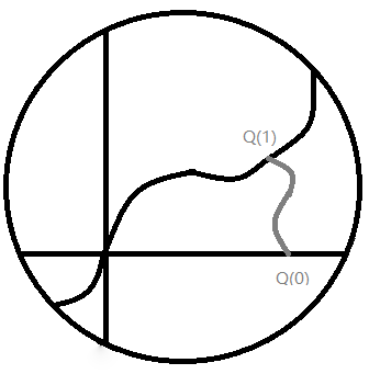
Figure 3.1. Fig.2 in [3]. The vertical line is $\Gamma_{\infty}$, horizonal lines are $\gamma_{0}$ and $\Sigma$. Gray line is the path $Q\left(t\right)$.

(See Figure 5,2.1) Choose a smooth path $Q\left(t\right),t\in\left[0,1\right]$ on $\mathbb{CP}^{2}-\Gamma_{\infty}$ such that $Q\left(0\right)\in\gamma_{0}$ and $Q\left(1\right)\in\Sigma$. There exists a smooth family of compatible almost complex structures $J\left(t\right),t\in\left[0,1\right]$ such that

$J\left(0\right)=J_{0}$

$\Sigma$ is $J\left(1\right)$-holomorphic

$\Gamma_{\infty}$ is $J\left(t\right)$-holomorphic for all t.

For the existence, one can first choose some appropriate almost complex structure along $\Gamma_{\infty}$, or say a section on the bundle of compatible actions over $\Gamma_{\infty}$. Since the space of compatible almost complex structures forms a contractible space, we can extend this section to $\mathbb{CP}^{2}$, which gives $J\left(t\right)$.

By Theorem 8, there exists a unique $J\left(t\right)-$holomorphic line, denoted by $C\left(t\right)$ passing through $P$ and $Q\left(t\right)$ changing smoothly w.r.t. parameter $t$. The deformation $\left\{C\left(t\right),t\in\left[0,1\right]\right\}$ gives an isotopy between $\gamma_{0}$ and $\Sigma$.

Before we finally extend $\left\{C\left(t\right),t\in\left[0,1\right]\right\}$ to an ambient isotopy of $\mathbb{CP}^{2}$ which preserves $\Gamma_{\infty}$, it remains to show that $C\left(t\right)$ intersects $\Gamma_{\infty}$ at the unique point $P$ transversally. If not,namely $C\left(t\right)$ intersect $\Gamma_{\infty}$ at more than one points(counted by multiplicity), by positivity of intersection in dim 4, each of them contributes positively to the intersection number $C\left(t\right)\cdot\Gamma_{\infty}$, so the number is bigger than one. However, $C\left(0\right)\cdot\Gamma_{\infty}=1$, contradicts the fact that the intersection number should remain unchanged for homologus lines.

Additionally, after a smooth deformation of $Q\left(t\right)$, one can require that for all $t\in\left[0,1\right]$, $Q\left(t\right)\cap\gamma_{0}$ not only at the point $x_{o}$, but also in a neighborhood $I\subset\gamma_{0}$ of $x_{0}$. Here it’s important that $Q\left(t\right)$ is transverse to $\Gamma_{\infty}$. Then one can make the isotopy intersect $I\times\Gamma_{\infty}$ only at $I$, thus obtain a compactly supported isotopy. ∎

4. Local Unknottedness of One-punctured Planar Lagrangians

4.1. The Nearby Lagrangian conjecture for the cylinder

We first explain the statement of [6, Theorem B] and show that this is actually equivalent to the nearby Lagrangian conjecture for the cylinder.

By cutting a torus $\mathbb{T}^{2}=\left(S^{1}\times S^{1}\right)$ parameterized by $\theta_{1}$ and $\theta_{2}$ between $\left\{\theta_{2}=s\right\}$ and $\left\{\theta_{2}=t\right\}$, we get two cylinders. This motivates us to realize that a Lagrangian cylinder inside the cotangent bundle of $T^{*}\left(S^{1}\times I\right)$ which is standard near the boundary can be extended to a Lagrangian torus in $T^{*}\left(S^{1}\times S^{1}\right)$ which is equal to the zero section in ${\theta_{2}\in\left[-\delta,\delta\right]}$ in the base. Namely, this isotopy of a Lagrangian torus keeps $S^{1}\times e^{i\left[-\delta,\delta\right]}$ fixed, so it is actually an isotopy of the rest part of a torus, which is a cylinder. We start by recalling the following result.

Theorem 16.

([6, Theorem B(2)], 2019) Suppose that $L\subset(T^{*}\mathbb{T}^{2},d\lambda_{\mathbb{T}^{2}})$ is an exact Lagrangian embedding. Then for any $\theta\in S^{1}$ consider the properly embedded Lagrangian disc with one interior point removed

$$\dot{D}_{\mathbf{P}^{0}}\left(\theta\right):=\left(S^{1}\times\left\{\theta\right\}\right)\times\left(\left\{p_{1}^{0}\right\}\times(-\infty,p_{2}^{0}]\right)\subset\mathbb{T}^{2}\times\mathbb{R}^{2}=T^{*}\mathbb{T}^{2},$$

$$\mathbf{p}^{0}:=\left(p_{1}^{0},p_{2}^{0}\right)$$

If it is the case that

$$L\cap\dot{D}_{\mathbf{p}^{0}}\left(e^{is}\right)=\partial\dot{D}_{\mathbf{p}^{0}}\left(e^{is}\right)=S^{1}\times\left\{e^{is}\right\}\times\left\{\mathbf{p}^{0}\right\}$$

holds for all $\mid s\mid<\epsilon$, then the Hamiltonian isotopy can be assumed to be supported outside of the subset

$$\bigcup_{\mid s\mid<\delta}\dot{D}_{\mathbf{p}^{0}}\left(e^{is}\right):=S^{1}\times e^{i\left[-\delta,\delta\right]}\times\left\{p_{1}^{0}\right\}\times(-\infty,p_{2}^{0}]$$

for some $0<\delta<\epsilon$ sufficiently small (note that for symplectic action reasons, we may not be able to Hamiltonian isotope the Lagrangian to the constant section $\mathbb{T}^{2}\times\left\{\mathbf{p}^{0}\right\}$).

The above result can in particular be applied to the torus which is an extension of a Lagrangian cylinder in $T^{*}\left(S^{1}\times I\right)$ which is standard above the boundary. However, we need to strengthen it in the following manner: make sure that the Hamiltonian isotopy of the torus is fixed above the entire subset $\theta_{2}\in\left[-\delta,\delta\right]$.

We prove the following strengthening of the result,

Theorem 17.

(The nearby Lagrangian conjecture for the cylinder) Let $L\subset T^{*}\mathbb{T}^{2}$ be an exact Lagrangian torus which coincides with the zero section above the subset $\theta_{2}\in\left[-\delta,\delta\right]$. Then $L$ is Hamiltonian isotopic to the zero section by a Hamiltonian isotopy which is supported in the same subset.

Proof.

We follow exactly the same steps as the proof of theorem B in [6, Section 9].

We prove by constructing a solid torus with core removed which is foliated by pseudo-holomorphic punctured discs.

The main step of the proof is to construct a proper embedding of a solid torus $\dot{\mathcal{T}}\subset T^{*}T^{2}$ with its core removed, which is foliated by pseudoholomorphic discs, and whose boundary is the Lagrangian $L$. For technical reasons this solid torus with core removed is constructed as a solid torus $\mathcal{T}\subset\mathbb{CP}^{1}\times\mathbb{CP}^{1}$ foliated by pseudoholomorphic discs, which gives rise to $\dot{\mathcal{T}}$ after removing the four holomorphic lines $\left(\left\{0,\infty\right\}\times\mathbb{CP}^{1}\right)\cup\left(\mathbb{CP}^{1}\times\left\{0,\infty\right\}\right)$. Recall that the complement of this divisor is a neighbourhood of the zero section of $T^{*}T^{2}$. In order to obtain the solid torus with the sought properties it is crucial that we have a family of (punctured) pseudoholomorphic discs that we can start with. Namely, one starts from the family of punctured pseudo-holomorphic discs

$$C\left(e^{is}\right)=S^{1}\times\left\{e^{is}\right\}\times\left(-\infty,p_{1}^{0}\right)\times\left\{p_{2}^{0}\right\}\subset T^{*}\mathbb{T}^{2}\setminus L$$

with boundary on $L$ that exists by the assumption that $L$ is standard above the neighborhood $\theta_{2}\in\left(-\delta,\delta\right)$. We proceed to explain how the additional assumptions made in Theorem 16 here give us additional control over the solid torus, as compared to the assumptions in Theorem 15 above which was proven in [6]. The goal is to use positivity of intersection to say that $\mathcal{\dot{T}}$ is standard above the region $\theta_{2}\in\left(-\delta,\delta\right)$.

In [6, Theorem B(2)], the condition about the intersection with the Lagrangian disc $\dot{D}_{\mathbf{P}^{0}}\left(\theta\right)$, says that the Hamiltonian isotopy is “one-sided” fixed near some Lagrangian disc, in the sense that the subset $\cup_{\mid s\mid<\delta}\dot{D}_{\mathbf{P}^{0}}\left(e^{is}\right)$ contains only $p_{2}<p_{2}^{0}$, but not $p_{2}>p_{2}^{0}$ and $p_{2}=p_{2}^{0}$. As in Section 9.1 of [6], denote a smooth one-dimensional family of embedded symplectic cylinders by

$$C\left(e^{is}\right)=S^{1}\times\left\{e^{is}\right\}\times\left(-\infty,p_{1}^{0}\right)\times\left\{p_{2}^{0}\right\}\subset T^{*}\mathbb{T}^{2}\setminus L$$

where $L$ is the Lagrangian torus, and for $p_{2}<p_{2}^{0}$, $p_{2}>p_{2}^{0}$, there are cylinders

$$C\left(p_{2},e^{is}\right)=S^{1}\times\left\{e^{is}\right\}\times\mathbb{R}\times\left\{p_{2}^{0}\right\}\subset T^{*}\mathbb{T}^{2}\setminus L.$$

Together, we can find a well-defined compatible almost complex structure $J$ on $\left(T^{*}\mathbb{T}^{2}\setminus L,d\lambda_{\mathbb{T}^{2}}\right)$ which is cylindrical outside of a compact subset, and which agrees with $J_{cyl}$ in a neighborhood of the union of cylinders. In [6], only $p_{2}<p_{2}^{0}$ was considered, however, if we look at Figure 5,2.16 in [6], there is also space for cylinders corresponds to $p_{2}>p_{2}^{0}$ above the $p_{2}$ plane. This property is a direct consequence of the assumption that $L$ coincides with the zero section above $\theta_{2}\in\left[-\delta,\delta\right]$.

Let us consider the family of cyliders

$$C\left(e^{is}\right)\cup C\left(p_{2},e^{is}\right),\mid s\mid\leq\delta,p_{2}<p_{2}^{0},p_{2}>p_{2}^{0}.$$

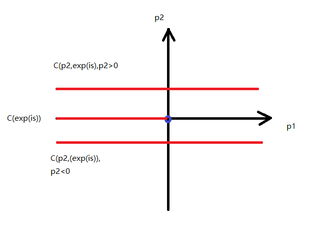
Figure 4.1. Figure 16 in [6], where the blue origin point is the only intersection, red lines are leaves of $\mathcal{\dot{T}}$.

The argument in [6, Section 9] produces an embeded solid torus $\mathcal{\dot{T}}$ inside $T^{*}\mathbb{T}^{2}$ with core removed, whose boundary is $L$, and which is foliated by pseudo-holomorphic cylinders with boundary on $L$. Part of these cylinders are given by the explicitly constructed standard cylinders $C\left(e^{is}\right)$. After compactifying $T^{*}\mathbb{T}^{2}$ to $S^{2}\times S^{2}$, $\mathcal{\dot{T}}$ becomes a solid torus. The positivity of intersection argument in Lemma 9.8(2) of [6] which shows that the solid torus is disjoint from $C\left(p_{2},e^{is}\right)$ also shows that the interior of these solid tori (which are foliated by pseudo-holomorphic curves) are disjoint from the cylinders $C\left(p_{2},e^{is}\right)$. In particular this solid torus coinsides with the union of standard cylinders $C\left(e^{is}\right)$ at origin but not in $p_{1}>0,p_{2}=0$ inside the subset $\theta_{2}\in\left[-\delta,\delta\right]$, because if so, either it is contained inside the domain, or it intersects the domain at a discrete subset. The former is impossible, by compactness, and the latter is also impossible, because it will also intersect the nearby cylinders $C\left(p_{2},e^{is}\right)$ by continuity. Hence $\mathcal{\dot{T}}$, and the isotopy, intersects

$$C\left(e^{is}\right)\cup C\left(p_{2},e^{is}\right),\mid s\mid\leq 4\delta,p_{2}<p_{2}^{0},p_{2}>p_{2}^{0}$$

exactly at the origin(s) of the Figure, in other words, we get an isotopy of the cylinder which is supported in the cotangent bundle of the cylinder. ∎

5. Local Unknottedness of Two-punctured Planes

While the analog of Theorem 9 for one-punctured planes (i.e. cylinder) is shown in Section 4.1, namely any Lagrangian inside $T^{*}\left(\mathbb{R}^{2}-\left\{0\right\}\right)$ which coincides with the zero-section outside of a compact subset is Hamiltonian isotopic to the zero section, the analogous result for $T^{*}\left(\mathbb{R}^{2}-\left\{0,1\right\}\right)$ (i.e. pair of pants) is unknown. Rather than Hamiltonian isotopy, we will try to prove the smooth version in this section.

Observe that here “compact” requires the isotopy to be fixed not only near $\infty$, but also 0 and 1. So we add back 0-fibre and 1-fibre, use the same idea of modification of $\omega$ to make the Lagrangian symplectic and compactification as the non-punctured case to construct an isotopy fixed at infinity. However, more needs to be done to make this isotopy fixed near 0 and 1. As an analog of Lemma 11 and 12, we have

Lemma 18.

There exists a diffeomorphism of $T^{*}\mathbb{R}^{2}=\mathbb{R}^{4}$ which takes the zero section to the complex line $\gamma_{0}$, the Lagrangian $L$ to a symplectic surface which coincides with a complex line $\gamma_{0}$ outside a compact subset, while the fibres over $0$ and $1$ become mapped to two disjoint symplectic lines $\Gamma_{0}$ and $\Gamma_{1}$, respectively, that intersects $\gamma_{0}$ transversely and positively in a single point, each are complex near $\gamma_{0}$ and outside a compact subset.

Proof.

First, we perturb $L$ to a symplectic surface $\alpha$ equal to $\gamma_{0}$, (i.e. the zero section, which is a symplectic linear plane for the symplectic form $\omega_{\varepsilon}$) near fibres and outside a compact subset. We construct this perturbation by an application of Moser’s trick as in Section 3, on a closed tubular neighborhood $V$ of $L$, one can find a closed 2-form $\tau$ such that there exists a 1-form $\lambda$ which is compactly supported on $V$ and vanishing near the fibres $\sigma_{0}=\left\{q_{1}=q_{2}=0\right\},\sigma_{1}=\left\{q_{1}=1,q_{2}=0\right\}$ with

$$d\lambda=\tau-dq_{1}\land dq_{2},$$

which coincides with $dq_{1}\land dq_{2}$ outside a compact subset of $V$ and makes $L$ $\tau-$symplectic. Choose a bump function $\rho$ on $\mathbb{R}^{4}$ which vanishes outside $V$, near the Lagrangian fibres $\sigma_{0}=\left\{q_{1}=q_{2}=0\right\},\sigma_{1}=\left\{q_{1}=1,q_{2}=0\right\}$, and equals 1 near the neighborhood where $L$ is Lagrangian. Set

$$\widetilde{\omega_{\varepsilon}^{\prime}}=\omega+\varepsilon\left(dq_{1}\land dq_{2}+d\left(\rho\lambda\right)\right).$$

Then $L$ is $\widetilde{\omega_{\varepsilon}^{\prime}}$-symplectic. Use Moser’s trick to deform $L$ to an $\omega_{\varepsilon}$-symplectic plane $\alpha$ by a smooth isotopy which is supported in the complement of $\sigma_{0}$, $\sigma_{1}$ defined above.

Second, we perturb Lagrangian fibres to symplectic planes. This can be done via a family of parallel 2-planes that intersect $\alpha$ transversely at two points. Namely, in the standard linear space $\mathbb{R}^{4}$ with coordinates $\left(p_{1},q_{1},p_{2},q_{2}\right)$ such that the symplectic form

$$\omega_{\varepsilon}=\left(dp_{1}-\frac{\varepsilon}{2}dq_{2}\right)\wedge dq_{1}+\left(dp_{2}+\frac{\varepsilon}{2}dq_{1}\right)\wedge dq_{2}$$

Consider a family of parallel pair of 2-planes $\Gamma_{0}^{t}$, $\Gamma_{1}^{t}$:

$$\Gamma_{0}^{t}:=\left\{\left(q_{1},q_{2}\right)^{T}=t\left(\begin{array}[]{cc}0&1\\ -1&0\end{array}\right)\cdot\left(p_{1},p_{2}\right)^{T}+\left(0,0\right)\right\}$$

$$\Gamma_{1}^{t}:=\left\{\left(q_{1},q_{2}\right)^{T}=t\left(\begin{array}[]{cc}0&1\\ -1&0\end{array}\right)\cdot\left(p_{1},p_{2}\right)^{T}+\left(1,0\right)\right\}$$

where $\Gamma_{0}^{0}$ is the Lagrangian fibre $\sigma_{0}=\left\{q_{1}=q_{2}=0\right\}$, and $\Gamma_{1}^{0}=\sigma_{1}=\left\{q_{1}=1,q_{2}=0\right\}.$ When $t=0$, $\Gamma_{0}^{0}$, $\Gamma_{1}^{0}$ are a pair of Lagrangian planes for the symplectic form $\omega_{\varepsilon}$, when $0<t\leq t_{0}$ for some $t_{0}>0$ small, $\Gamma_{0}^{t}$, $\Gamma_{1}^{t}$ are a pair of symplectic planes for the symplectic form $\omega_{\varepsilon}$. If needed, one can rescale the $p_{i}$ coordiantes to flatten the Lagrangian $L$ so that $\Gamma_{0}^{t}$, $\Gamma_{1}^{t}$ will not intersect $L$ at points other than our desired two transversal intersection points.

Third, map $\gamma_{0}$ to the complex line $\mathbb{C}\times 0$ by a linear symplectomorphism. Meanwhile, denote the symplectic images of $\gamma_{0}$, $\Gamma_{0}^{t_{0}}$, $\Gamma_{1}^{t_{0}}$ by the same notations. One can obtain a smooth family $\Sigma_{s}$ of symplectic immersions, where $\Sigma_{0}=\gamma_{0}\cup\Gamma_{0}^{t_{0}}\cup\Gamma_{1}^{t_{0}}$ with fixed intersection points $pt_{0},pt_{1}$ on $\Gamma_{0}^{t_{0}}$, $\Gamma_{1}^{t_{0}}$ respectively.

Finally, use [6, Proposition 4.9] to obtain a new deformation $\widetilde{\Sigma_{t}}$ through symplectic immersions with exactly two transverse double points, such that $\widetilde{\Sigma_{0}}=\Sigma_{0}$ and that the deformation fixes $\gamma_{0}$ and the positions $pt_{0}$ and $pt_{1}$ of the double points and where the deformation has support near the double points and near $\infty$. After such a deformation we may assume that the sought properties are satisfied. ∎

Again as Lemma 12, take an interpolerated symplectic form and compactify $\mathbb{R}^{4}$ into $\left(\mathbb{CP}^{2},\Omega,J_{0}\right)$ by adding $\Gamma_{\infty}$. The complex lines $\Gamma_{0}$, $\Gamma_{1}$ from the previous proposition become symplectic spheres in the projective plane. Denote them again by $\Gamma_{0}$, $\Gamma_{1}$. Moreover, we may assume that this $J_{0}$ makes $\gamma_{0}$$,\Gamma_{0},\Gamma_{1},\Gamma_{\infty}$ simultaneously J-holomorphic. The symplectic plane $\alpha$ becomes an embedded symplectic sphere, denoted by $\alpha$ again, which intersects $\Gamma_{\infty}$, $\Gamma_{0}$, $\Gamma_{1}$ at the same points as $\gamma_{0}$ does. Denote the intersections by $\infty,$ $pt_{0}$, $pt_{1}$ respectively. See Figure 5,1. In the following we abuse notation and use $\Gamma_{0}$, $\Gamma_{1}$ in order to denote the compactifications of the symplectic planes to symplectic degree one spheres in $\mathbb{CP}^{2}.$

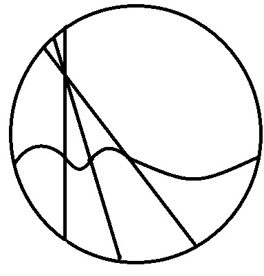
Figure 5.1. Vertical lines are $\Gamma_{\infty}$, $\Gamma_{0}$, $\Gamma_{1}$, they intersect at the same point $x_{0}$. The horizonal line is $\alpha$ which intersect $\Gamma_{\infty}$, $\Gamma_{0}$, $\Gamma_{1}$ at $\infty,$ $pt_{0}$, $pt_{1}$ respectively.

Note the following: $\Gamma_{i}$ are complex planes which are linear outside a compact subset and near $\mathbb{C}\times 0.$ The key point to our proof is that we can interpolate through compatible almost complex structures that keep $\Gamma_{\infty}$, $\Gamma_{0}$, $\Gamma_{1}$ J-holomorphic, from one that makes $\alpha$ J-holomorphic, to one that makes $\gamma_{0}$ J-holomorphic.

Theorem 19.

There exists a smooth isotopy of $\mathbb{CP}^{2}$ that takes $\alpha$ to $\gamma_{0}$ which fixes the line $\Gamma_{\infty}$ pointwise, keeps the intersection point between this isotopy’s image and $\Gamma_{\infty}$, $\Gamma_{0}$, $\Gamma_{1}$ at $\infty,$ $pt_{0}$, $pt_{1}$ respectively, and the image does not intersect $\Gamma_{\infty}$, $\Gamma_{0}$, $\Gamma_{1}$ at other points. Moreover, this isotopy can be taken to fix a neighborhood of $\Gamma_{\infty}$, $\Gamma_{0}$, $\Gamma_{1}$.

Proof.

By Lemma 18, we have an almost complex structure $J_{0}$ making $\gamma_{0},\Gamma_{0},\Gamma_{1},\Gamma_{\infty}$ simultaneously $J_{0}$-holomorphic. There is also an almost complex structure $J_{1}$ making $\alpha,\Gamma_{0},\Gamma_{1},\Gamma_{\infty}$ simultaneously $J_{1}$-holomorphic, again as argued in Theorem 14 by extending a section of a bundle with contractible fibres. Choose the path $J_{t}$ of almost complex structures for which $\Gamma_{0},\Gamma_{1},\Gamma_{\infty}$ remain $J_{t}$-holomorphic for all times t. Consider the unique $J_{t}$-holomorphic line, denoted by $\alpha_{t}$, passing through the two intersection points $\infty,0$. We have $\alpha_{0}=\gamma_{0}$, $\alpha_{1}=\alpha$ and the family $\left\{\alpha_{t},0\leq t\leq 1\right\}$ gives the smooth isotopy from $\alpha$ to $\gamma_{0}$. One can extend this isotopy to an isotopy of $\mathbb{CP}^{2}$ that fixes $\Gamma_{0},\Gamma_{1},\Gamma_{\infty}$, by [6, Proposition 4.8]. However, the problem is that $\alpha_{t}$ may not intersect $\Gamma_{1}$ at 1. See Figure 5,2.

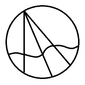
Figure 5.2. The intersection points of $\alpha_{t}$ and $\Gamma_{\infty}$, $\Gamma_{0}$ is $\infty$ and $pt_{0}$ respectively, but the intersection of $\alpha_{t}$ and $\Gamma_{1}$may not be $pt_{1}$.

Use parameter $t$ to denote the above isotopy process $f\left(t,x\right),t\in\left[0,1\right],x\in\mathbb{CP}^{2}$ from $\alpha$ to $\gamma_{0}$, with Figure 5,2 as an intermediate status between them.

For every tamed $J$, $\mathbb{CP}^{2}-\left\{x_{0}\right\}$ can be foliated by $J-$holomorphic spheres that all intersect at $x_{0}$. Especially, there is a unique $J_{t}$-holomorphic curve passing through $x_{0}$ and $1$, denoted by $\Gamma^{t}$. There is a smooth isotopy for each $t\in\left[0,1\right]$ that takes $\Gamma_{1}$ to $\Gamma^{t}$. Parameterize this isotopy by $s$. Together we have an isotopy

$$g\left(t,s,x\right),t\in\left[0,1\right],s\in\left[0,1\right],x\in\mathbb{CP}^{2}$$

with the property that $g\left(0,s,x\right)=x$, $g\left(1,s,x\right)=x$. Take the top-path of the two-dimensional domain of $\left(s,t\right)$, we get the desired smooth isotopy. See Figure 5.3.

Figure 5.3. The two-dimendional domain of the parameter pair $\left(t,s\right)$.

Parameterize this path by $r$, finally we get a smooth isotopy from $\alpha$ to $\gamma_{0}$, which keeps the intersection points $\infty,$$\Gamma_{0}^{t_{0}}$, $\Gamma_{1}^{t_{0}}$. By the same intersection argument as in section 3, this isotopy intersect $\Gamma_{\infty}$, $\Gamma_{0}$, $\Gamma_{1}$ at no other points.

A standard topological argument like that in the end of Proposition 12 makes the smooth isotopy away from $\Gamma_{\infty}$, $\Gamma_{0}$, $\Gamma_{1}$. Moreover, one can use the method of [6, Theorem 4.6] to make the isotopy also symplectic. ∎

References

- [1] Arnol’d, V. I. (1986). First steps in symplectic topology. Russian Mathematical Surveys, 41(6), 1-21.
- [2] Gromov, M. (1985). Pseudo holomorphic curves in symplectic manifolds. Inventiones mathematicae, 82(2), 307-347.
- [3] Eliashberg, Y., & Polterovich, L. (1997). The problem of Lagrangian knots in four-manifolds. Geometric topology (Athens, GA, 1993), 2, 313-327.
- [4] Eliashberg, Y., & Polterovich, L. (1996). Local Lagrangian 2-knots are trivial. Annals of mathematics, 144(1), 61-76.
- [5] Eliashberg, Y., & Polterovich, L. (1993). Unknottedness of Lagrangian surfaces in symplectic 4-manifolds. International Mathematics Research Notices, 1993(11), 295-301.
- [6] Dimitroglou Rizell, G. (2019). The classification of Lagrangians nearby the Whitney immersion. Geometry & Topology, 23(7), 3367-3458.
- [7] Côté, L., & Rizell, G. D. (2020). Symplectic Rigidity of Fibers in Cotangent Bundles of Riemann Surfaces. arXiv preprint arXiv:2004.04233.
- [8] McDuff, D., & Salamon, D. (2017). Introduction to symplectic topology. Oxford University Press.
- [9] McDuff, D., & Salamon, D. (2012). J-holomorphic curves and symplectic topology (Vol. 52). American Mathematical Soc..
- [10] Wendl, C. (2010). Lectures on holomorphic curves in symplectic and contact geometry. arXiv preprint arXiv:1011.1690.
- [11] McDuff, D. (1994). Singularities and positivity of intersections of J-holomorphic curves. In Holomorphic curves in symplectic geometry (pp. 191-215). Birkhäuser, Basel.
- [12] Moser, J. (1965). On the volume elements on a manifold. Transactions of the American Mathematical Society, 120(2), 286-294.