Holographic charm and bottom pentaquarks I
Mass spectra with spin effects

Abstract

We revisit the three non-strange pentaquarks $[\frac{1}{2}\frac{1}{2}^{-}]_{S=0,1}$ and $[\frac{1}{2}\frac{3}{2}^{-}]_{S=1}$ predicted using the holographic dual description, where chiral and heavy quark symmetry are manifest in the triple limit of a large number of colors, large quark mass and strong ^′t Hooft gauge coupling. In the heavy quark limit, the pentaquarks with internal heavy quark spin $S$ are all degenerate. The holographic pentaquarks are dual to an instanton bound to heavy mesons in bulk, without the shortcomings related to the nature of the interaction and the choice of the hard core inherent to the molecular constructions. We explicitly derive the spin-spin and spin-orbit couplings arising from next to leading order in the heavy quark mass, and lift totally the internal spin degeneray, in fair agreement with the newly reported charmed pentaquarks from LHCb. New charm and bottom pentaquark states are predicted.

I Introduction

Recently the LHCb collaboration has revisited its analysis of the pentaquark states using a nine-fold increase in reconstructed $\Lambda_{b}^{0}\rightarrow J/\Psi pK^{-}$ decays from the LHCb Run-2 data batch at 13 TeV Aaij et al. (2019). The LHCb new high statistics analysis shows that the previously reported $P_{c}^{+}(4450)$ Aaij et al. (2015) splits into two narrow peaks $P_{c}^{+}(4440)$ and $P_{c}^{+}(4457)$ below the $\Sigma_{c}^{+}\bar{D}^{*0}$ threshold, with the appearance of a new and narrow $P_{c}^{+}(4312)$ state below the $\Sigma_{c}^{+}\bar{D}^{0}$. The evidence for the previously reported state $P_{c}^{+}(4380)$ Aaij et al. (2015) has weakened.

We regard the new LHCb data as evidence that supports the three lowest non-strange pentaquarks with spin-isospin assignments $[\frac{1}{2}\frac{1}{2}^{-}]_{S=0,1}$ and $[\frac{1}{2}\frac{3}{2}^{-}]_{S=1}$ predicted by holography Liu and Zahed (2017a), in the triple limit of a large number of colors, strong ^′t Hooft gauge coupling and a large quark mass. More importantly, we will show below that the degeneracy in the internal heavy quark spin $S=1$, is lifted by spin-orbit effects at next to leading order in the heavy quark mass as heavy quark symmetry is broken, in fair agreement with the new data. Furthermore, we regard the closeness of the pentaquarks $P_{c}^{+}(4457)$ and $P_{c}^{+}(4312)$ to the $\Sigma_{c}^{+}\bar{D}^{*0}$ and $\Sigma_{c}^{+}\bar{D}^{0}$ tresholds respectively, as further evidence in support of this construction, as both tresholds coalesce in the heavy quark limit.

Pentaquark states with hidden charm were initially suggested in Wu et al. (2010); Karliner and Rosner (2015), and since have been addressed by many  Burns (2015); Richard (2016); Lebed et al. (2017); Esposito et al. (2017); Olsen et al. (2018); Guo et al. (2018); Karliner et al. (2018) (and references therein). In short, the current descriptions range from pentaquarks made of compact diquarks Maiani et al. (2015); Lebed (2015), to hadro-charmonia Eides et al. (2020) and loosely bound hadronic molecules Du et al. (2021) (and references therein). Heavy pentaquarks as multiquark states composed of heavy and light quarks, fall outside the realm of the canonical quark model. Their description calls for a novel hadronic paradigm with manifest chiral and heavy quark symmetry.

It is well established that chiral symmetry dictates most of the interactions between light quarks, while heavy quark symmetry organizes the spin interactions between heavy quarks Shuryak (1982); Isgur and Wise (1991). Both symmetries are inter-twined by the phenomenon of chiral doubling Nowak et al. (1993); Bardeen and Hill (1994); Nowak et al. (2004) as shown experimentally in Aubert et al. (2003); Besson et al. (2003). Therefore, a theoretical approach to the multiquark states should have manifest chiral and heavy quark symmetry, a clear organizational principle in the confining regime, and should address concisely the multi-body bound state problem.

The holographic principle in general Maldacena (1999); Erlich et al. (2005), and the D4-D8-D$\bar{8}$ holographic set-up in particular Sakai and Sugimoto (2005) provide a framework for addressing QCD in the infrared in the double limit of a large number of colors and strong ^′t Hooft gauge coupling $\lambda=g_{YM}^{2}N_{c}$. It is confining and exhibits spontaneous chiral symmetry breaking geometrically. The light meson sector is well described by an effective action with manifest chiral symmetry and very few parameters, yet totally in line with more elaborate effective theories of QCD Fujiwara et al. (1985). The same set-up can be minimally modified to account for the description of heavy-light mesons, with manifest heavy quark symmetry Liu and Zahed (2017b, a, c); Li (2017); Fujii and Hosaka (2020).

Light and heavy-light baryons are dual to instantons and instanton-heavy meson bound states in bulk Hata et al. (2007); Hashimoto et al. (2008); Kim and Zahed (2008); Hata and Murata (2008); Hashimoto et al. (2010); Lau and Sugimoto (2017), providing a robust geometrical approach to the multi-body bound state problem. The holographic construction provides a dual realization of the chiral soliton approach and its bound states variants Zahed and Brown (1986); Rho et al. (1992); Rho and Zahed (2017), without the shortcomings of the derivative expansion. It is a geometrical realization of the molecular approach  Wu et al. (2010); Karliner and Rosner (2015), without the ambiguities of the nature of the meson exchanges, and the arbitrariness in the choice of the many couplings and form factors Lin and Zou (2019). Alternative holographic models for the description of heavy hadrons have been developed in Dosch et al. (2015); Sonnenschein and Weissman (2019).

The organization of the paper is as follows: in section II we recall the essential aspects of the $N_{f}=2$ heavy light effective action in leading order in the heavy quark mass introduced in Liu and Zahed (2017b, a). In section III we extend this analysis at next to leading order in the heavy quark mass for the bound heavy baryons seeded by instantons in bulk. In section IV we detail the spin-orbit and spin-spin effects for the heavy baryons and their exotics. The induced quantum effective potentials are made explicit in section V. In section VI we derive the holographic mass formula for the heavy-light baryons and their exotic pentaquarks including the spin contributions. By adjusting the chief Kaluza-Klein scale used in Liu and Zahed (2017a, c), a more refined heavy baryon spectrum emerges, including the newly reported charmed pentaquarks by LHCb. Our conclusions are in section VII. A number of Appendices are added to support the various results.

II Holographic heavy-light effective action

The D4-D8-D$\bar{8}$ set-up for light flavor branes is standard Sakai and Sugimoto (2005). The minimal modification that accommodates heavy mesons makes use of an extra heavy brane as discussed in Liu and Zahed (2017b, a, c). It consists of $N_{f}$ light D8-D$\bar{8}$ branes (L) and one heavy (H) probe brane in the cigar-shaped geometry that spontaneously breaks chiral symmetry. We assume that the L-brane world volume consists of $R^{4}\times S^{1}\times S^{4}$ with $[0-9]$-dimensions. The light 8-branes are embedded in the $[0-3+5-9]$-dimensions and set at the antipodes of $S^{1}$ which lies in the 4-dimension. The warped $[5-9]$-space is characterized by a finite size $R$ and a horizon at $U_{KK}$.

II.1 Dirac-Born-Infeld (DBI) action

The effective action on the probe L-branes consists of the non-Abelian DBI and Chern-Simons action. After integrating over the $S^{4}$, the leading contribution in $1/\lambda$ to the DBI action is

$$S_{\rm DBI}\approx-\kappa\int d^{4}xdz\,{\rm Tr}\left({\bf f}(z){\bf F}_{\mu\nu}{\bf F}^{\mu\nu}+{\bf g}(z){\bf F}_{\mu z}{\bf F}^{\nu z}\right)\ .$$ (1)

The warping factors are

$${\bf f}(z)=\frac{R^{3}}{4U_{z}}\,,\qquad{\bf g}(z)=\frac{9}{8}\frac{U_{z}^{3}}{U_{KK}}\ ,$$ (2)

with $U_{z}^{3}=U_{KK}^{3}+U_{KK}z^{2}$, and $\kappa\equiv a\lambda N_{c}$ and $a=1/(216\pi^{3})$ Sakai and Sugimoto (2005). All dimensions are in units of $M_{KK}$ (Kaluza-Klein scale) unless given explicitly. Our conventions are $(-1,1,1,1,1)$ with $A_{M}^{\dagger}=-A_{M}$ and the labels $M,N$ running over $\mu,z$ only in this section. The effective fields in the field strengths are Liu and Zahed (2017b, a)

$${\bf F}_{MN}=\left(\begin{array}[]{cc}F_{MN}-\Phi_{[M}\Phi_{N]}^{\dagger}&\partial_{[M}\Phi_{N]}+A_{[M}\Phi_{N]}\\ -\partial_{[M}\Phi^{\dagger}_{N]}-\Phi^{\dagger}_{[M}A_{N]}&-\Phi^{\dagger}_{[M}\Phi_{N]}\end{array}\right)\ .$$ (5)

The matrix valued 1-form gauge field is

$${\bf A}=\left(\begin{array}[]{cc}A&\Phi\\ -\Phi^{\dagger}&0\end{array}\right)\ ,$$ (6)

For $N_{f}=2$, the naive Chern-Simons 5-form is

$$S_{CS}=\frac{iN_{c}}{24\pi^{2}}\int_{M_{5}}\,{\rm Tr}\left(AF^{2}-\frac{1}{2}A^{3}F+\frac{1}{10}A^{5}\right)\ .$$ (7)

We note that for only $N_{f}>2$ it fails to reproduce the correct transformation law under the combined gauge and chiral transformations Hata and Murata (2008). In particular, when addressing the $N_{f}=3$ baryon spectra, (7) does not reproduce the important hypercharge constraint Hata and Murata (2008), but can be minimally modified to do that.

For $N_{f}$ coincidental branes, the $\Phi$ multiplet is massless, but for separated branes they are massive with the additional contribution

$$\frac{1}{2}m_{H}^{2}{\rm Tr}\left(\Phi^{\dagger}_{M}\Phi_{M}\right)\ .$$ (8)

The value of $m_{H}$ is related to the separation between the light and heavy branes, which is about the length of the HL string. It is related to the heavy meson masses $M_{D}=1870$ MeV (charmed) and $M_{B}=5279$ MeV (bottomed) through Liu and Zahed (2017b)

$$M_{D,B}=m_{H}+\frac{M_{KK}}{2\sqrt{2}}\ .$$ (9)

Given $M_{KK}$ and $M_{D,B}$, the mass parameter $m_{H}$ is therefore totally fixed.

II.2 Light fields

In the coincidental brane limit, light baryons are interchangeably described as a flavor instanton or a D4 brane wrapping the $S^{4}$. The instanton mass is $M_{0}=8\pi^{2}\kappa$ in units of $M_{KK}$. The instanton size is small with $\rho\sim 1/\sqrt{\lambda}$ after balancing the order $\lambda$ bulk gravitational attraction with the subleading and of order $\lambda^{0}$ U(1) induced topological repulsion Sakai and Sugimoto (2005). The bulk instanton is described by the O(4) gauge field

$$A_{M}(y)=-\overline{\sigma}_{MN}\partial_{N}F(y)\qquad\left.F_{zm}(y)\right|_{|y|=R}=0\ .$$ (10)

From hereon $M,N$ run only over $1,2,3,z$ unless specified otherwise. If $\rho\sim 1/\sqrt{\lambda}$ is the typical size of these tunneling configurations, then it is natural to recast the DBI action using the rescaling

$$(x_{0},x_{M})\rightarrow(x_{0},x_{M}/\sqrt{\lambda}),\sqrt{\lambda}\rho\rightarrow\rho\qquad\qquad(A_{0},A_{M})\rightarrow(A_{0},\sqrt{\lambda}A_{M})$$ (11)

The rescaled fields satisfy the equations of motion

$$D_{M}F_{MN}=0\qquad\partial_{M}^{2}A_{0}=-\frac{1}{32\pi^{2}a}F_{aMN}\star{F}_{aMN}\ ,$$ (12)

with the use of the Hodge dual notation.

II.3 Heavy-light fields

Let $(\Phi_{0},\Phi_{M})$ be the pair of heavy quantum fields that bind to the tunneling configuration above. If again $\rho\sim 1/\sqrt{\lambda}$ is their typical size, then it is natural to recast the heavy-light part of the DBI action using the additional rescaling

$$(\Phi_{0},\Phi_{M})\rightarrow(\Phi_{0},\sqrt{\lambda}\Phi_{M})\ .$$ (13)

The interactions between the light gauge fields $(A_{0},A_{M})$ and the heavy fields $(\Phi_{0},\Phi_{M})$ to quadratic order split to several contributions Liu and Zahed (2017b, a)

$${\cal L}=aN_{c}\lambda{\cal L}_{0}+aN_{c}{\cal L}_{1}+{\cal L}_{CS}\ .$$ (14)

which are quoted in (58). We start by recalling the leading contributions in $1/m_{H}$ stemming from (14) as thoroughly discussed in Liu and Zahed (2017a, c). For that, we split $\Phi_{M}=\phi_{M}e^{-im_{H}x_{0}}$ for particles ($m_{H}\rightarrow-m_{H}$ for anti-particles). The leading order contribution takes the form

$${\cal L}_{0}=-\frac{1}{2}\left|f_{MN}-\star f_{MN}\right|^{2}+2\phi_{M}^{\dagger}(F_{MN}-\star F_{MN})\phi_{N}\ ,$$ (15)

subject to the constraint equation $D_{M}\phi_{M}=0$ with

$$f_{MN}=\partial_{[M}\phi_{N]}+A_{[M}\phi_{N]}\ ,$$ (16)

while the subleading contributions in (14) to order $\lambda^{0}m_{H}$ simplify to

$$\frac{{\cal L}_{1}}{aN_{c}}\rightarrow 4m_{H}\phi^{\dagger}_{M}iD_{0}\phi_{M}\qquad\qquad{\cal L}_{CS}\rightarrow\frac{m_{H}N_{c}}{16\pi^{2}}\phi^{\dagger}_{M}\star F_{MN}\phi_{N}\ .$$ (17)

For self-dual light gauge fields with $F_{MN}=\star F_{MN}$, the last contribution in (15) vanishes, and the minimum is reached for $f_{MN}=\star f_{MN}$. This observation when combined with the transversality condition for $D_{M}\phi_{M}=0$, amounts to a first order equation for the combination $\psi=\bar{\sigma}_{M}\phi_{M}$ with $\sigma_{M}=(i,\vec{\sigma})$, i.e.

$$\sigma_{M}D_{M}\psi=D\psi=0\ ,$$ (18)

as noted in Liu and Zahed (2017b, a). In a self-dual gauge configuration, the heavy spin-1 meson transmutes to a massless spin-$\frac{1}{2}$ spinor that is BPS bound in leading order.

III The order ${1}/{m_{H}^{2}}$ Lagrangian

To account for the spin effects and the breaking of heavy quark symmetry we need to account for the $1/m_{H}$ contributions to (14-17). This will be sought by restricting the quantum and heavy fields to the quantum moduli. More specifically, we choose to parametrize the fields using

$$A_{M}(t,x)=V(A_{M}^{cl}-i\partial_{M})V^{-1},\qquad A_{0}(t,x)=0$$

$$\Phi_{M}(t,x)=\frac{e^{-im_{H}t}}{\sqrt{16m_{H}aN_{c}}}V(t,x)f(X(t),Z(t))\bar{\sigma}_{M}\chi(t)\ .$$ (19)

which is equivalent to

$$A_{M}(t,x)=A_{M}^{cl}(X(t),Z(t)),\qquad A_{0}(t,x)=-iV\partial_{t}V^{-1}\equiv\Phi$$

$$\Phi_{M}(t,x)=f(X(t),Z(t))\bar{\sigma}_{M}\chi(t)\ .$$ (20)

after gauge transformation. The $\Phi$ is parameterized as

$$\Phi=-\dot{X}_{N}A^{\rm cl}_{N}+\chi^{a}\Phi_{a}\ ,$$ (21)

where $\Phi_{a}$ diagonalizes $D_{M}^{\rm cl}D_{M}^{\rm cl}\Phi_{a}$ and where

$$\chi^{a}={\rm tr}(\tau^{a}{\bf a}^{-1}\dot{\bf a})\ ,$$ (22)

are expressed in terms of the collective variables ${\bf a}\in{\rm SU(2)}$ for a rigid ${\rm SU(2)}$ rotation. The temporal component $\Phi_{0}$ satisfies the constraint

$$(-D_{M}^{2}+m_{H}^{2})\Phi_{0}+2F_{M0}\Phi_{M}-\frac{i}{16\pi^{2}a}F_{PQ}(\partial_{P}+A_{P})\Phi_{Q}=0\ .$$ (23)

and in leading order in $1/m_{H}$ can be ignored.

Inserting the expansion (III) in (58) yields the quadratic $1/m_{H}$ contributions,

$${\cal L}_{\rm quadratic}=\frac{1}{8m_{H}}\chi^{\dagger}\sigma_{M}f(\partial_{t}-A_{0}-\Phi)(\partial_{t}-A_{0}-\Phi)\bar{\sigma}_{M}f\chi-\tilde{\cal L}_{1}+\tilde{\cal L}_{\rm CS}\ ,$$ (24)

Here $\tilde{\cal L}_{\rm CS}$ contains only $\Phi_{M}$. Each of the contribution in (24) is discussed in Appendix A. Combining the results (78,107,113) we have for the quadratic contributions to order $\frac{1}{m_{H}}$

$${\cal L}_{\rm quadratic}= \frac{1}{m_{H}}\bigg{(}\frac{c_{1}}{\pi^{4}a^{2}\rho^{4}}\chi^{\dagger}\chi+i\frac{c_{2}}{\pi^{2}a\rho^{2}}\chi^{\dagger}\dot{\chi}+i\frac{c_{3}}{\pi^{2}a\rho^{2}}\chi^{\dagger}\tau^{a}\chi\chi^{a}+\frac{\dot{\chi}^{\dagger}\dot{\chi}}{2}\bigg{)}$$

$$-\frac{37+12\frac{Z^{2}}{\rho^{2}}}{192m_{H}}\chi^{\dagger}\chi+\left(\frac{1}{4m_{H}}\frac{\dot{\rho}^{2}}{\rho^{2}}+\frac{\dot{a}_{I}^{2}}{4m_{H}}+\frac{\dot{X}^{2}}{4m_{H}\rho^{2}}\right)\chi^{\dagger}\chi\ ,$$ (25)

with the constants fixed to

$$c_{1}=\frac{13}{3840}+\frac{7}{1280}=\frac{17}{1920}\ ,$$

$$c_{2}=\frac{2}{32}\ ,$$

$$c_{3}=\frac{1}{128}+\frac{1}{80}=\frac{13}{640}\ .$$ (26)

In the mean time, one has also to take into account the Chern-Simons term contribution

$$-\frac{i}{16\pi^{2}}\epsilon_{MNPQ}\Phi^{\dagger}_{M}\Phi_{N}\Phi^{\dagger}_{P}\partial_{t}\Phi_{Q}+{\rm c.c.}\ ,$$ (27)

which is

$${\cal L}_{\rm quartic,CS}=-\frac{N_{c}}{5m_{H}m_{y}^{2}\rho^{4}}\chi^{\dagger}\tau^{a}\chi\chi^{\dagger}\tau^{a}\chi\ ,$$ (28)

where $m_{y}=16\pi^{2}a$.

The above analysis ignores the Coulomb back reaction (repulsion from the bound charged fields) as we discussed in Liu and Zahed (2017b, a) and can lead to instabilities. In Appendix B we detail the back-reaction from the Coulomb field with the final result for (III) to order ${\cal O}({1}/{m_{H}^{2}})$

$${\cal L}\rightarrow\,\, i\chi^{\dagger}\dot{\chi}+\frac{1}{2m_{H}}\dot{\chi}^{\dagger}\dot{\chi}+\frac{78}{5m_{H}\tilde{\rho}^{2}}i\chi^{\dagger}\tau^{a}\chi\chi^{a}-\frac{12}{5m_{H}\tilde{\rho}^{4}}\vec{S}^{2}-\frac{37+12\frac{Z^{2}}{\rho^{2}}}{192m_{H}}n$$

$$+\frac{1}{\tilde{\rho}^{2}}\bigg{(}-\frac{18}{5}+\frac{9}{2}n-\frac{2}{3}n^{2}\bigg{)}+\frac{1}{m_{H}\tilde{\rho}^{4}}\bigg{(}\frac{102}{5}n-\frac{56}{5}n^{2}+\frac{4}{3}n^{3}+j\tilde{\rho}^{2}\left(\frac{9}{2}-\frac{4n}{3}\right)\bigg{)}$$

$$+\frac{1}{m_{H}^{2}\tilde{\rho}^{6}}\bigg{(}-\frac{128n^{4}}{45}+\frac{376n^{3}}{15}-\frac{4017n^{2}}{70}-jn\tilde{\rho}^{2}\left(\frac{56}{5}-\frac{8}{3}n\right)-\frac{2}{3}j^{2}\tilde{\rho}^{4}\bigg{)}\ ,$$ (29)

with

$$j=\frac{i}{2}\left(\chi^{\dagger}\dot{\chi}-\dot{\chi}^{\dagger}\chi\right),\ n=\chi^{\dagger}\chi\ ,$$ (30)

This is the first major result of this paper. We now study the quantization of the (III) and the ensuing heavy-light baryonic spectra.

IV Quantum spin effects

IV.1 Spin-orbit effect

The first major spin contribution occurs through the spin-angular momentum coupling $\chi^{a}\chi^{\dagger}\tau^{a}\chi$. Recall that $\chi^{a}$ in modular variables is

$$\chi^{a}=2i(a_{4}\dot{a}_{a}-\dot{a}_{4}a_{a}+\epsilon_{abc}a_{b}\dot{a}_{c})\ ,$$ (31)

with $a_{4}^{2}+\sum_{a=1}^{3}a_{a}^{2}=1$ parametrizing the $SU(2)\sim S^{3}$ moduli. Thus, the canonical momenta for $y_{I}$ read

$$\Pi_{a}=m_{y}\rho^{2}\dot{a}_{a}-\frac{2c_{3}}{m_{H}\pi^{2}a\rho^{2}}(a_{4}\chi^{\dagger}\tau_{a}\chi+\epsilon_{cba}\chi^{\dagger}\tau_{c}\chi a_{b})\ ,$$ (32)

$$\Pi_{4}=m_{y}\rho^{2}\dot{a}_{4}+\frac{2c_{3}}{m_{H}\pi^{2}a\rho^{2}}\chi^{\dagger}\tau_{a}\chi a_{a}\ ,$$ (33)

Therefore the spin-orbit contribution to the Hamiltonian is

$$H= \frac{1}{2m_{y}\rho^{2}}(-i\nabla_{\rm S^{3}}+\frac{4c_{3}}{m_{H}\pi^{2}a\rho^{2}}\vec{r}\times\vec{S})^{2}$$

$$= \frac{-\nabla^{2}_{\rm S_{3}}}{2m_{y}\rho^{2}}+\frac{8c_{3}}{m_{H}\pi^{2}a\rho^{2}}\frac{\vec{L}\cdot\vec{S}}{m_{y}\rho^{2}}+\bigg{(}\frac{4c_{3}}{m_{H}\pi^{2}a\rho^{2}}\bigg{)}^{2}\frac{\chi^{\dagger}\frac{\vec{\tau}}{2}\chi\cdot\chi^{\dagger}\frac{\vec{\tau}}{2}\chi}{2m_{y}\rho^{2}}\ ,$$ (34)

with the orbital angular momentum

$$\vec{L}=\frac{1}{2}\left(i\vec{a}\nabla_{4}-ia_{4}\vec{\nabla}-i\vec{a}\times\vec{\nabla}\right)\ ,$$ (35)

The integer-valued spin of the heavy-light doublet translates to a half-integer spin on the moduli

$$\vec{S}=\chi^{\dagger}\frac{\vec{\tau}}{2}\chi\ ,$$ (36)

a remarkable transmutation induced by the binding of the zero mode to the instanton in bulk Liu and Zahed (2017b). To leading order in ${1}/{m_{H}}$ only the first two contributions in (IV.1) will be retained. The last contribution in (IV.1) is the induced spin-spin interaction of the heavy mesons and is suppressed by $1/m_{H}^{2}$.

IV.2 Spin effects

The leading spin effects to order $1/m_{H}$ stem from the quadratic and quartic $\chi$-contributions detailed above. The terms with a first order time-derivative of $\chi$ are

$$(1+\frac{3N_{c}}{2m_{H}m_{y}\rho^{2}})i\chi^{\dagger}\dot{\chi}+\frac{\dot{\chi}^{\dagger}\dot{\chi}}{2m_{H}}-i\frac{2\chi^{\dagger}\chi(\chi^{\dagger}\dot{\chi}-\dot{\chi}^{\dagger}\chi)}{3m_{H}m_{y}\rho^{2}}\ ,$$ (37)

and imply the equation of motion

$$-\frac{1}{2m_{H}}\partial_{t}^{2}\chi+i(1+\frac{3N_{c}}{2m_{H}m_{y}\rho^{2}})\partial_{t}\chi+\frac{3N_{c}}{2m_{y}\rho^{2}}\chi+\frac{4i(\chi^{\dagger}\chi\dot{\chi}+\chi^{\dagger}\dot{\chi}\chi)}{3m_{H}m_{y}\rho^{2}}=0\ .$$ (38)

Therefore to second order in ${1}/{m_{H}}$ one has

$$i\partial_{t}\chi= -\frac{3N_{c}}{2m_{y}\rho^{2}}\chi+\frac{9N_{c}^{2}}{8m_{H}m_{y}^{2}\rho^{4}}\chi+\frac{4\chi^{\dagger}\chi\chi N_{c}}{m_{H}m_{y}^{2}\rho^{4}}$$

$$+ \frac{81N_{c}^{3}}{32m_{H}^{2}m_{y}^{3}\rho^{6}}\chi-\frac{32N_{c}(\chi^{\dagger}\chi)^{2}\chi}{3m_{H}^{2}m_{y}^{2}\rho^{6}}\ ,$$ (39)

from which the Hamiltonian can be easily extracted.

IV.3 Hamiltonian

With the above in mind and to obtain the Hamiltonian in leading order in ${1}/{m_{H}}$, it is sufficient to perform the following substitution

$$j\rightarrow-\frac{3N_{c}}{2\tilde{\rho}^{2}}\ ,$$ (40)

and add

$$\delta H=\frac{81}{8m_{H}\tilde{\rho}^{4}}n+\frac{1}{m_{H}^{2}\tilde{\rho}^{6}}\left(\frac{81N_{c}^{3}}{32}n-\frac{32N_{c}}{9}n^{3}\right)\ ,$$ (41)

to the the spin-independent Hamiltonian Liu and Zahed (2017b).

More specifically, for a single heavy-quark with $n=1$, the total Hamiltonian to order ${1}/{m_{H}}$ now reads ($N_{c}=3$)

$$H_{\rm single} = \frac{39\vec{L}\cdot\vec{S}}{5m_{H}m_{y}^{2}(1+\frac{1}{2m_{H}m_{y}\rho^{2}})\rho^{4}}+\bigg{(}-\frac{553}{120m_{H}m_{y}^{2}\rho^{4}}+\frac{67.94}{m_{H}^{2}m_{y}^{4}\rho^{6}}+\frac{37+12\frac{Z^{2}}{\rho^{2}}}{192m_{H}}\bigg{)}$$

$$- \frac{1}{2m_{y}\rho^{3}(1+\frac{1}{2m_{H}m_{y}\rho^{2}})^{2}}\frac{\partial}{\partial\rho}\left(\rho^{3}(1+\frac{1}{2m_{H}m_{y}\rho^{2}})\frac{\partial}{\partial\rho}\right)+\frac{4\vec{L}^{2}}{2m_{y}\rho^{2}(1+\frac{1}{2m_{H}m_{y}\rho^{2}})}\ ,$$

The change in the Laplacian is due to the $\frac{\dot{\rho}^{2}}{\rho^{2}}+a_{I}^{2}$ term following from the new line element on the moduli

$$ds^{2}=(1+\frac{1}{2m_{H}m_{y}\rho^{2}})dy_{I}^{2}\ ,$$ (43)

with a change in the small $\rho$ behavior. For the penta-quark states where $N_{\bar{Q}}=N_{Q}=1$, the corresponding Hamiltonian is ($N_{c}=3$)

$$H_{\rm double} = \frac{39\vec{L}\cdot\vec{S}}{5m_{H}m_{y}^{2}(1+\frac{1}{m_{H}m_{y}\rho^{2}})\rho^{4}}+\bigg{(}-\frac{411}{20m_{H}m_{y}^{2}\rho^{4}}+\frac{133.30}{m_{H}^{2}m_{y}^{4}\rho^{6}}+\frac{37+12\frac{Z^{2}}{\rho^{2}}}{96m_{H}}\bigg{)}$$ (44)

$$- \frac{1}{2m_{y}\rho^{3}(1+\frac{1}{m_{H}m_{y}\rho^{2}})^{2}}\frac{\partial}{\partial\rho}\left(\rho^{3}(1+\frac{1}{m_{H}m_{y}\rho^{2}})\frac{\partial}{\partial\rho}\right)+\frac{4\vec{L}^{2}}{2m_{y}\rho^{2}(1+\frac{1}{m_{H}m_{y}\rho^{2}})}\ .$$

Below we solve the corresponding Schroedinger equation numerically.

V Induced quantum potentials

V.1 The effective potential for single-heavy quark: $l=0$ state

For $l=0$, the spin-orbit coupling vanishes, i.e. $\vec{L}\cdot\vec{S}=0$, and the induced effective potential simplifies to

$$V(\rho)=\frac{m_{y}\omega_{\rho}^{2}}{2}\rho^{2}-\frac{7}{30m_{y}\rho^{2}}+\bigg{(}-\frac{553}{120m_{H}m_{y}^{2}\rho^{4}}+\frac{67.94}{m_{H}^{2}m_{y}^{4}\rho^{6}}\bigg{)}\ .$$ (45)

Although the sign of the $\frac{1}{\rho^{2}}$ is negative, the $m_{H}=\infty$ system is still stable due to the uncertainty principle. Indeed, for small $\rho$, the kinetic contribution is of order $\frac{1}{\rho^{2}}$ and compensates the negative sign to maintain stability. In this case, the ${1}/{m_{H}}$ term implies additional repulsion that further stabilizes the system. As $m_{H}\rightarrow\infty$, the spectrum approaches the infinite mass limit smoothly.

V.2 The effective potential for single-heavy quark: $l>0$ state

For $l=2,4,..$, one has $J=(l\pm 1)/2$. We first consider the $J=(l-1)/2$ case. Again for $N_{Q}=1$ and $N_{c}=3$, the effective potential reads

$$V\bigg{(}J=\frac{l-1}{2},\rho\bigg{)} = \frac{1}{2m_{y}(1+\frac{1}{2m_{H}m_{y}\rho^{2}})\rho^{2}}\left(l(l+2)-\frac{(l+2)\alpha N_{c}}{m_{H}m_{y}\rho^{2}}+\frac{3\alpha^{2}N_{c}^{2}}{4m_{H}^{2}m_{y}^{2}\rho^{4}}\right)$$ (46)

$$+ \frac{m_{y}\omega_{\rho}^{2}}{2}\rho^{2}-\frac{7}{30m_{y}\rho^{2}}+\bigg{(}-\frac{553}{120m_{H}m_{y}^{2}\rho^{4}}+\frac{67.94}{m_{H}^{2}m_{y}^{4}\rho^{6}}\bigg{)}\ ,$$

with $\alpha=\frac{13}{10}$. The ${1}/{m_{H}^{2}}$ term due to the spin-orbit coupling is kept to maintain stability at small $\rho$. The change of the potential as one increases $m_{H}$ tends to decrease for larger $l$. For $l=2$, the shapes of the potential at $m_{H}=2$ and $m_{H}=\infty$ differ moderately, but for $l=2$ the difference is already quite small.

Similarly, in the $J=\frac{l+1}{2}$ case the effective potential is

$$V\bigg{(}J=\frac{l+1}{2},\rho\bigg{)} = \frac{1}{2m_{y}(1+\frac{1}{2m_{H}my\rho^{2}})\rho^{2}}\left(l(l+2)+\frac{l\alpha N_{c}}{m_{H}m_{y}\rho^{2}}+\frac{3\alpha^{2}N_{c}^{2}}{4m_{H}^{2}m_{y}^{2}\rho^{4}}\right)$$ (47)

$$+ \frac{m_{y}\omega_{\rho}^{2}}{2}\rho^{2}-\frac{7}{30m_{y}\rho^{2}}+\bigg{(}-\frac{553}{120m_{H}m_{y}^{2}\rho^{4}}+\frac{67.94}{m_{H}^{2}m_{y}^{4}\rho^{6}}\bigg{)}\ .$$

Again, the $1/m_{H}$ contribution further stabilizes the system and pushes the spectrum a little bit higher.

V.3 The effective potential for penta-quark state

Here we focus on the pentaquark states with $N_{Q}=\bar{N}_{Q}=1$ state or hidden $Q=c,b$, with $S=0,1$. For $S=0$, the potential reads

$$V\bigg{(}J=\frac{l}{2},S=0\bigg{)}=\frac{m_{y}\omega_{\rho}^{2}\rho^{2}}{2}+\frac{18}{5m_{y}\rho^{2}}+\frac{l(l+2)}{2m_{y}(1+\frac{1}{m_{H}m_{y}^{2}\rho^{2}})\rho^{2}}+\bigg{(}-\frac{411}{20m_{H}m_{y}^{2}\rho^{4}}+\frac{133.30}{m_{H}^{2}m_{y}^{4}\rho^{6}}\bigg{)}\ ,$$ (48)

For $S=1$ we can have $J=l-1,l,l+1$, and the potential in this case reads

$$V(J,S=1,\rho) = \frac{1}{2m_{y}(1+\frac{1}{m_{H}m_{y}^{2}\rho^{2}})\rho^{2}}\left(l(l+2)+\frac{2N_{c}\Delta(J)\beta}{m_{H}m_{y}\rho^{2}}+\frac{2N_{c}^{2}\beta^{2}}{m_{H}^{2}m_{y}^{2}\rho^{4}}\right)+\frac{18}{5m_{y}\rho^{2}}$$ (49)

$$+ \frac{m_{y}\omega_{\rho}^{2}}{2}\rho^{2}+\bigg{(}-\frac{411}{20m_{H}m_{y}^{2}\rho^{4}}+\frac{133.30}{m_{H}^{2}m_{y}^{4}\rho^{6}}\bigg{)}\ .$$

with $\beta=\frac{13}{10}$ and

$$\Delta(J)=J(J+1)-\frac{l(l+2)}{4}-2\ .$$ (50)

More specifically, for $l=1$ we have $\Delta(J=1/2)=-2$ and $\Delta(J=3/2)=1$.

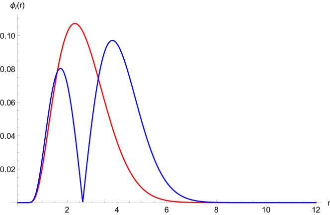
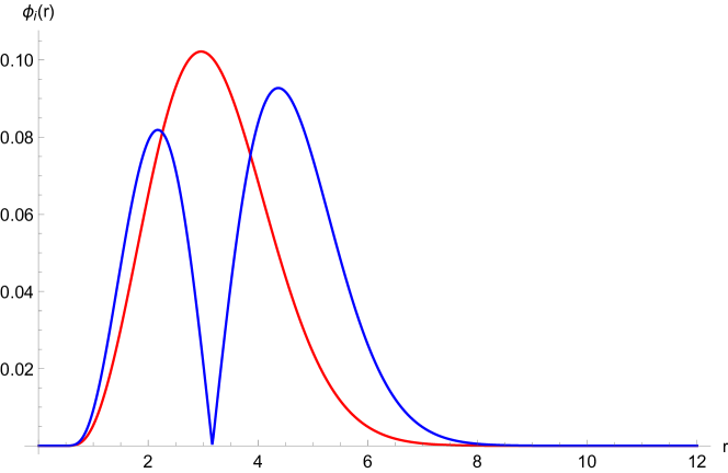
Figure 1: The $l=0$ radial wave functions for single heavy-baryon (top) and double-heavy-baryon or penta-quark state (bottom). See text.

VI Spectra

Given the Hamiltonian and the explicit induced quantum potentials, we can now obtain the spectra of the holographic heavy-light hadrons. Our strategy is the following: we treat the warping contribution as a small perturbation, while solving the radial part numerically. For the warping part, using the average

$$\left<\frac{Z^{2}}{\rho^{2}}\right>_{n_{z},n_{\rho}}=\frac{n_{z}+\frac{1}{2}}{\tilde{l}+1}\ ,$$ (51)

we obtain

$$\delta M_{\rm wrap}=\frac{37+\frac{6}{\tilde{l}+1}}{192m_{H}}(N_{Q}+N_{\bar{Q}})\ ,$$ (52)

in unit of $M_{KK}$.

To obtain the radial part, we need to solve the Schroedinger equation

$$-\frac{1}{2m_{y}\rho^{3}(1+\frac{1}{2m_{H}m_{y}\rho^{2}})^{2}}\frac{\partial}{\partial\rho}\left(\rho^{3}\bigg{(}1+\frac{1}{2m_{H}m_{y}\rho^{2}}\bigg{)}\frac{\partial}{\partial\rho}\right)\Psi_{n,l}(\rho)+V_{l}(\rho)\Psi_{n,l}(\rho)=E_{n,l}\Psi_{n,l}(\rho)\ ,$$ (53)

with the warped normalization condition

$$2\pi^{2}\int_{0}^{\infty}\rho^{3}\bigg{(}1+\frac{1}{2m_{y}\rho^{2}}\bigg{)}^{2}|\Psi_{n,l}(\rho)|^{2}d\rho=1\ .$$ (54)

For this purpose we perform the transformation $\Psi\rightarrow u$ and use $\tilde{\rho}^{2}=m_{y}\rho^{2}$

$$\Psi=\frac{u}{\sqrt{\rho^{3}(1+\frac{1}{2m_{H}m_{y}\rho^{2}})}}\ ,$$ (55)

to simplify (53)

$$-\frac{1}{2(1+\frac{1}{2m_{H}\tilde{\rho}^{2}})}u_{n,l}^{\prime\prime}(\tilde{\rho})+\bigg{[}\frac{3\big{(}1+\frac{1}{m_{H}\rho^{2}}-\frac{1}{12m_{H}^{2}\tilde{\rho}^{4}}\big{)}}{8\tilde{\rho}^{2}(1+\frac{1}{2m_{H}\tilde{\rho}^{2}})}\bigg{]}u_{n,l}(\tilde{\rho})+V_{l}(\tilde{\rho})u_{n,l}(\tilde{\rho})=E_{n,l}u_{n,l}(\tilde{\rho})\ ,$$ (56)

with the normalization condition

$$2\pi^{2}\int_{0}^{\infty}d\tilde{\rho}\bigg{(}1+\frac{1}{2m_{H}\tilde{\rho}^{2}}\bigg{)}|u_{n,l}(\tilde{\rho})|^{2}=1\ .$$ (57)

Notice that the normalization condition actually requires the $u_{n,l}$ to vanish near $\tilde{\rho}$. In this case one can show that although the additional term ( large bracket in (53) ) becomes negative at small $\tilde{\rho}$, the spectrum $E_{n,l}$ is still bounded from below. The above equation for $u_{n,l}$ can be diagonalized numerically and below we present the results for different states.

Table 1: Charm baryons and Pentaquarks

$B$	$IJ^{P}$	$l$	$n_{\rho}$	$n_{z}$	$N_{Q}$	$N_{\bar{Q}}$	Mass-MeV	Exp-MeV
$\Lambda_{c}$	$0{\frac{1}{2}}^{+}$	0	0	0	1	0	2286	2286
$\Sigma_{c}$	$1{\frac{1}{2}}^{+}$	2	0	0	1	0	2557	2453
	$1{\frac{3}{2}}^{+}$	2	0	0	1	0	2596	2520
$\Lambda^{*}_{c}$	$0{\frac{1}{2}}^{-}$	0	0	1	1	0	2683	2595
	$0{\frac{1}{2}}^{+}$	0	1	0	1	0	2726	2765
$\Sigma^{*}_{c}$	$1{\frac{1}{2}}^{-}\,,\,1{\frac{3}{2}}^{-}$	2	0	1	1	0	[2947/2986]	–
	$1{\frac{1}{2}}^{+}\,,\,1{\frac{3}{2}}^{+}$	2	1	0	1	0	[2948/2995]	–
$P_{c}$	$\frac{1}{2}{\frac{1}{2}}^{-}\,,\,\frac{1}{2}{\frac{3}{2}}^{-}$	1	0	0	1	1	[4340/4360/4374]	[4312/4440/4457]
$P^{*}_{c}$	$1{\frac{1}{2}}^{-}\,,\,1{\frac{3}{2}}^{-}$	1	0	1	1	1	[4732/4752/4767]	–
	$1{\frac{1}{2}}^{+}\,,\,1{\frac{3}{2}}^{+}$	1	1	0	1	1	[4725/4746/4763]	–

Table 2: Bottom baryons and Pentaquarks

$B$	$IJ^{P}$	$l$	$n_{\rho}$	$n_{z}$	$N_{Q}$	$N_{\bar{Q}}$	Mass-MeV	Exp-MeV
$\Lambda_{b}$	$0{\frac{1}{2}}^{+}$	0	0	0	1	0	5608	5620
$\Sigma_{b}$	$1{\frac{1}{2}}^{+}$	2	0	0	1	0	5962	5810
	$1{\frac{3}{2}}^{+}$	2	0	0	1	0	5978	5830
$\Lambda^{*}_{b}$	$0{\frac{1}{2}}^{-}$	0	0	1	1	0	5998	5912
	$0{\frac{1}{2}}^{+}$	0	1	0	1	0	6029	(6072)
$\Sigma^{*}_{b}$	$1{\frac{1}{2}}^{-}\,,\,1{\frac{3}{2}}^{-}$	2	0	1	1	0	[6351/6367]	–
	$1{\frac{1}{2}}^{+}\,,\,1{\frac{3}{2}}^{+}$	2	1	0	1	0	[6344/6367]	–
$P_{b}$	$\frac{1}{2}{\frac{1}{2}}^{-}\,,\,\frac{1}{2}{\frac{3}{2}}^{-}$	1	0	0	1	1	[11155/11163/11167]	–
$P^{*}_{b}$	$1{\frac{1}{2}}^{-}\,,\,1{\frac{3}{2}}^{-}$	1	0	1	1	1	[11544/11553/11556]	–
	$1{\frac{1}{2}}^{+}\,,\,1{\frac{3}{2}}^{+}$	1	1	0	1	1	[11532 /11543/11579]	–

To fix the parameters for the charmed heavy baryons, we choose $M_{D}=1.87$ GeV for the D-meson mass in (9) and fix $M_{KK}=0.475$ GeV to reproduce the $M_{\Lambda_{c}}=2.286$ GeV. This low value of $M_{KK}$ is consistent with the value used to reproduce the nucleon spectra Hata et al. (2007), but about half the value of $M_{KK}\sim 1$ GeV used originally in Sakai and Sugimoto (2005) and adopted in Liu and Zahed (2017b, a, c). In this case we have $m_{H}=(1.87-0.168)$ GeV= $3.66M_{KK}$. In Fig. 1 we show the radial wavefunctions for the first and second excited states following from (53) for a single heavy-baryon (top) and doubly heavy-baryon or pentaquark state (bottom). Note the rapid decay of the wavefunctions near the instanton core as $\rho\rightarrow 0$.

The corresponding charm and bottom states for single- and double-heavy hadrons are listed in Table 1 and Table 2 respectively. Note that while $m_{\Lambda_{c}}=2.286$ GeV is fitted to fix the Kaluza-Klein scale $M_{KK}=0.475$ GeV, $m_{\Lambda_{b}}=5.608$ GeV is a holographic prediction which is remarkably close to the experimental value of 5.620 GeV. The details of the mass budgets for each of the states in terms of the three holographic parameters, are given in Appendix C. The results for the single-heavy baryon spectrum are remarkable given the small number of parameters used in this holographic approach. The spin contributions improve considerably the predictions for the masses and their hierarchy. In particular, the empirical mass ordering $\Sigma_{c}-\Lambda_{c}<\Lambda_{c}^{*}-\Lambda_{c}$ is obtained contrary to the claim in Fujii and Hosaka (2020). The mass splitting between $\Sigma_{c}$ and $\Sigma_{b}$ is higher than observed due to the sizable repulsion from the $l=2$ intrinsic angular momentum assignment.

The holographic construction with spin corrections, allows for only three pentaquark states which are close to the observed charmed pentaquark states reported by LHCb, although with slightly smaller masses (the 80 MeV difference can be easily narrowed by adjusting the Kaluza-Klein scale $M_{KK}=0.475$ GeV at the expense of $\Lambda_{c}$). The spin-orbit effects split away the $[\frac{1}{2}\frac{1}{2}^{-}]_{S=1}$ and $[\frac{1}{2}\frac{3}{2}^{-}]_{S=1}$ states, lifting the degeneracy reported originally in Liu and Zahed (2017a). The present holographic construction rules out a pentaquark with $[\frac{1}{2}\frac{5}{2}^{\pm}]$ assignment since the instanton core carries equal spin-isospin Liu and Zahed (2017a). The splitting between the different pentaquark states are somehow smaller than expected, due to the strength of the spin-orbit coupling to order ${1}/{m_{H}^{2}}$. Additional contributions are expected to order ${1}/{m_{H}^{3}}$. This construction supports additional Roper-like and odd-parity-like pentaquark states which we have denoted by $P^{*}_{c,b}$, although heavier and mor susceptible to decay.

VII Conclusions

In the holographic construction presented in Liu and Zahed (2017b, a, c), heavy hadrons are described in bulk using a set of degenerate $N_{f}$ light D8-D$\bar{8}$ branes plus one heavy probe brane in the cigar-shaped geometry that spontaneously breaks chiral symmetry. This construction enforces both chiral and heavy-quark symmetry and describes well the low-lying heavy-light mesons and baryons. Heavy baryons are composed of heavy-light mesons bound to a core instanton in bulk. Remarkably, the bound heavy-light mesons with spin-1 transmute to heavy quarks with spin-$\frac{1}{2}$, an amazing spin-statistics transmutation by geometry.

In Liu and Zahed (2017b, a, c) the analysis of the bound states and spectra was carried to order $m_{H}^{0}$ where the spin effects are absent. In this work and for $N_{f}=2$, we have now carried the analysis at next to leading order in $1/m_{H}$ where the spin-orbit and spin corrections are manifest. By refining the Kaluza-Klein scale $M_{KK}$ from 1 GeV used in Liu and Zahed (2017a, c) to 0.475 GeV used here, a rich spectrum with single- and double-heavy baryons emerges with fair agreement with the empirically observed states, including the newly reported charm pentaquark states by LHCb.

This is remarkable, given that only three parameters were used in the holographic construction: $M_{0},M_{KK},m_{H}$. For charm, they are fixed by $M_{0}\rightarrow m_{N}$ (nucleon mass), $M_{KK}\rightarrow M_{\Lambda_{c}}$ (Lambda-mass) and $m_{H}\rightarrow M_{D}$ (D-meson mass). The only parameter adjustment for the bottom spectrum is $m_{H}\rightarrow M_{B}$ (B-meson mass). Needless to say that the light-light, heavy-light and heavy-heavy mesons and baryons are described simultaneously, without changing the number of parameters.

The holographic construction predicts a triplet of nearly degenerate charm pentaquark states with the isospin-spin-parity assignments

$$\bigg{(}\bigg{[}P_{c}(4340)\frac{1}{2}\frac{1}{2}^{-}\bigg{]}_{S=1},\bigg{[}P_{c}(4360)\frac{1}{2}\frac{1}{2}^{-}\bigg{]}_{S=0},\bigg{[}P_{c}(4374)\frac{1}{2}\frac{3}{2}^{-}\bigg{]}_{S=1}\bigg{)}$$

which are to be compared to $P_{c}[4312|4440|4457]$ recently reported by LHCb. The small mass discrepancy can be readily eliminated by adjusting the Kaluza-Klein scale at the expense of $\Lambda_{c}$. The spin-orbit effects split away the states with intrinsice spin $S=1$. The analysis rules out the assignment $[\frac{1}{2}\frac{5}{2}^{\pm}]$ for these states, and predicts a triplet of bottomed pentaquark states

$$\bigg{(}\bigg{[}P_{b}(11532)\frac{1}{2}\frac{1}{2}^{-}\bigg{]}_{S=1},\bigg{[}P_{b}(11543)\frac{1}{2}\frac{1}{2}^{-}\bigg{]}_{S=0},\bigg{[}P_{b}(11579)\frac{1}{2}\frac{3}{2}^{-}\bigg{]}_{S=1}\bigg{)}$$

not yet observed. New Roper-like and odd-parity pentaquark states are also suggested, although much heaviers and more susceptible to fall apart.

Finally, the present holographic description can be regarded as the holographic dual of the chiral soliton construction of heavy-light baryons Rho et al. (1992); Rho and Zahed (2017) (and references therein). However, in the latter the uncertainties in combining chiral and heavy quark symmetry strongly limit their predictive range, especially when addressing the spin corrections. This is not the case for the holographic description as we have shown, as both symmetries are geometrically embedded in the bulk brane construction with just three parameters. The dual approach is vastly superior.

Acknowledgements

This work is supported by the Office of Science, U.S. Department of Energy under Contract No. DE-FG-88ER40388 and by the Polish National Science Centre (NCN) Grant UMO-2017/27/B/ST2/01139.

Appendix A Details of the heavy mass expansion

Following the rescaling in (11) the effective action for the heavy-light fields split into the following contributions

$${\cal L}=aN_{c}\lambda{\cal L}_{0}+aN_{c}({\cal L}_{1}+\tilde{\cal L}_{1})+{\cal L}_{\rm CS}$$ (58)

with each contribution given by

$${\cal L}_{0}= -(D_{M}\Phi_{N}^{\dagger}-D_{N}\Phi_{M}^{\dagger})(D_{M}\Phi_{N}-D_{N}\Phi_{M})+2\Phi_{M}^{\dagger}F_{MN}\Phi_{N}\ ,$$

$${\cal L}_{1}= +2(D_{0}\Phi_{M}^{\dagger}-D_{M}\Phi_{0}^{\dagger})(D_{0}\Phi_{M}-D_{M}\Phi_{0})-2\Phi_{0}^{\dagger}F^{0M}\Phi_{M}$$

$$-2\Phi^{\dagger}_{M}F^{M0}\Phi_{0}-2m_{H}^{2}\Phi^{\dagger}_{M}\Phi_{M}\ ,$$

$$\tilde{\cal L}_{1}= +\frac{z^{2}}{3}(D_{i}\Phi_{j}-D_{j}\Phi_{i})^{\dagger}(D_{i}\Phi_{j}-D_{j}\Phi_{i})$$

$$-2z^{2}(D_{i}\Phi_{z}-D_{z}\Phi_{i})^{\dagger}(D_{i}\Phi_{z}-D_{z}\Phi_{i})-\frac{2}{3}z^{2}\Phi_{i}^{\dagger}F_{ij}\Phi_{j}+2z^{2}(\Phi^{\dagger}_{z}F_{zi}\Phi_{i}+c.c)\$$

$${\cal L}_{CS}= -\frac{iN_{c}}{16\pi^{2}}\Phi^{\dagger}(dA+A^{2})D\Phi-\frac{iN_{c}}{16\pi^{2}}(D\Phi)^{\dagger}(dA+A^{2})\Phi+{\cal O}(\Phi^{3})\ .$$ (59)

We now use the expansion (III) to explicitly derive the various contributions in (58) in leading order in $1/m_{H}$. The net result has manifest heavy quark symmetry to order $m_{H}^{0}$, with the spin-orbit and spin-spin contributions breaking this symmetry to order $1/m_{H}$.

A.1 Kinetic contribution: ${\cal L}_{\rm kin}$

The explicit form of the kinetic contribution is

$${\cal L}_{\rm kin}=\frac{1}{8m_{H}}\chi^{\dagger}\sigma_{M}f(-\partial_{t}-\hat{A}_{0}-\Phi)(\partial_{t}+\hat{A}_{0}+\Phi)\bar{\sigma}_{M}f\chi\ ,$$ (60)

which contains derivative of $\chi$. With the help of the identity for Weyl matrices $\sigma_{M}\tau^{a}\bar{\sigma}_{M}=0$, (60) reads

$$\frac{1}{2m_{H}}f^{2}\dot{\chi}^{\dagger}\dot{\chi}+\frac{1}{2m_{H}}\dot{X}_{N}\dot{X}_{M}\partial_{N}f\partial_{M}f\chi^{\dagger}\chi+\frac{f^{2}}{2m_{H}}\hat{A}_{0}(\dot{\chi}^{\dagger}\chi-\chi^{\dagger}\dot{\chi})-\frac{f^{2}}{2m_{H}}\hat{A}_{0}^{2}\chi^{\dagger}\chi-\frac{f^{2}}{4m_{H}}{\rm tr}(\Phi)^{2}\chi^{\dagger}\chi\ .$$ (61)

which can be further simplified by using the explicit relations

$$-{\rm tr}\Phi^{2}=\frac{X^{4}}{4(X^{2}+\rho^{2})^{2}}2\chi^{a\dagger}\chi^{a}-\dot{X}_{N}\dot{X}_{M}{\rm tr}A_{N}A_{M}=\frac{2X^{4}}{(X^{2}+\rho^{2})^{2}}\dot{a}_{I}^{2}+\frac{3X^{2}}{2(X^{2}+\rho^{2})^{2}}\dot{X}^{2}$$ (62)

and

$$\hat{A}_{0}=-\frac{i}{8\pi^{2}ax^{2}}\left(1-\frac{\rho^{4}}{(x^{2}+\rho^{2})^{2}}\right)\ .$$ (63)

to have

$${\cal L}_{\rm kin}$$

$$=\frac{\dot{\chi}^{\dagger}\dot{\chi}}{2m_{H}}+\left(\frac{1}{4m_{H}}\frac{\dot{\rho}^{2}}{\rho^{2}}+\frac{\dot{a}_{I}^{2}}{4m_{H}}+\frac{\dot{X}^{2}}{4m_{H}\rho^{2}}\right)\chi^{\dagger}\chi+\frac{1}{16m_{H}\pi^{2}a\rho^{2}}i\chi^{\dagger}\partial_{t}\chi+\frac{13}{3840m_{H}\pi^{4}a^{2}\rho^{4}}\chi^{\dagger}\chi$$ (64)

after integration over space.

A.2 Chern-Simons contribution: ${\cal L}_{\rm CS}$

The Chern-Simons term is

$${\cal L}_{\rm CS} =-\frac{iN_{c}}{16\pi^{2}}\Phi^{\dagger}(dA+A^{2})D\Phi-\frac{iN_{c}}{16\pi^{2}}(D\Phi)^{\dagger}(dA+A^{2})\Phi$$

$$=-\frac{iN_{c}}{8\pi^{2}}\Phi^{\dagger}(dA+A^{2})D\Phi$$ (65)

where in the second line we have performed a partial integration with the help of the Bianchi identity $DF=0$. More explicitly, we have

$$\frac{i}{128m_{H}\pi^{2}a}f^{2}\chi^{\dagger}\sigma_{M}F_{MN}\bar{\sigma}_{N}\dot{\chi}+\frac{i\epsilon_{MNPQ}}{128m_{H}\pi^{2}a}f\chi^{\dagger}\sigma_{M}F_{0N}(\partial_{P}+A_{P})f\bar{\sigma}_{Q}\chi$$

$$+\hat{A}_{0}\left(\frac{iN_{c}}{128m_{H}\pi^{2}a}\chi^{\dagger}\sigma_{M}F_{MN}\bar{\sigma}_{N}\chi f^{2}\right)\ ,$$ (66)

which is seen to contain $\chi^{\dagger}\chi$ as well as linear terms in derivatives. Recall that the electric field $F_{0M}$ after solving Gauss constraint reads

$$F_{0M}=\dot{X}_{N}F_{MN}+\dot{\rho}\frac{\partial A_{M}}{\partial\rho}-\chi^{a}D_{M}\Phi^{a}\ ,$$ (67)

The linear terms in $\dot{\rho}$, $\dot{X}_{N}$ vanish due to parity and translational invariance, but there are terms of the form

$$\chi^{a}\chi^{\dagger}\frac{\tau^{a}}{2}\chi=i\chi^{\dagger}{\bf a}^{-1}\dot{\bf a}\chi$$ (68)

which couple to isospin. Again, using the identity for Weyl matrices

$$\epsilon_{MNPQ}\bar{\sigma}_{QR}=-\delta_{MR}\bar{\sigma}_{MP}+\delta_{NR}\bar{\sigma}_{MP}-\delta_{PQ}\bar{\sigma}_{MN}\ ,$$ (69)

all terms that require anti-symmetrization vanish

$$-\epsilon_{MNPQ}\sigma_{M}F_{0N}\bar{\sigma}_{P}\partial_{Q}f=0\ ,$$ (70)

but the more involved one

$$-\epsilon_{MNPQ}\sigma_{M}F_{0N}A_{P}\bar{\sigma}_{Q}= \frac{\sigma_{M}F_{0N}\bar{\sigma}_{NQ}\bar{\sigma}_{Q}X_{M}}{X^{2}+\rho^{2}}-\frac{\sigma_{M}F_{0N}\bar{\sigma}_{MQ}\bar{\sigma}_{Q}X_{N}}{X^{2}+\rho^{2}}$$ (71)

$$+\frac{\sigma_{M}F_{0N}\bar{\sigma}_{MN}\bar{\sigma}_{Q}X_{Q}}{X^{2}+\rho^{2}}\ .$$

does not. Using the identity $\sigma_{M}\tau^{i}\bar{\sigma}_{M}=0$, the second term vanishes, while the first and the third term read

$$\frac{\sigma_{M}F_{0N}\bar{\sigma}_{NQ}\bar{\sigma}_{Q}X_{M}}{X^{2}+\rho^{2}}= \frac{3\sigma\cdot XF_{0N}\bar{\sigma}_{N}}{X^{2}+\rho^{2}}=-\frac{9\rho^{2}f}{(X^{2}+\rho^{2})^{2}}\tau^{a}\chi^{a}\ ,$$

$$\frac{\sigma_{M}F_{0N}\bar{\sigma}_{MN}\bar{\sigma}_{Q}X_{Q}}{X^{2}+\rho^{2}}= -\frac{\sigma_{M}F_{0N}\bar{\sigma}_{N}\sigma_{M}\bar{\sigma}\cdot X}{2(X^{2}+\rho^{2})}=\frac{3\rho^{2}f}{(X^{2}+\rho^{2})^{2}}\tau^{a}\chi^{a}\ ,$$ (72)

Since

$$-\epsilon_{MNPQ}\sigma_{M}F_{0N}A_{P}\bar{\sigma}_{Q}=-\frac{6\rho^{2}f}{(X^{2}+\rho^{2})^{2}}\tau^{a}\chi^{a}\ .$$ (73)

we finally have

$$-\epsilon_{MNPQ}\Phi^{\dagger}_{M}F_{0N}D_{P}\Phi_{Q}=-\frac{6\rho^{2}f^{2}}{16m_{H}N_{c}a(X^{2}+\rho^{2})^{2}}\chi^{\dagger}\tau^{a}\chi\chi^{a}\ .$$ (74)

One should also consider the contribution from $\hat{F}_{0N}=-\frac{1}{r}\frac{\partial{\hat{A}}_{0}}{\partial r}x_{N}$,

$$-\epsilon_{MNPQ}\sigma_{M}\hat{F}_{0N}A_{P}\bar{\sigma}_{Q}=\frac{6X^{2}}{X^{2}+\rho^{2}}\frac{1}{r}\frac{\partial\hat{A}_{0}}{\partial r}\,$$ (75)

The final Chern-Simons contribution to order $1/m_{H}$ after rescaling is

$$\frac{3}{16m_{H}\pi^{2}a}\frac{f^{2}\rho^{2}}{(X^{2}+\rho^{2})^{2}}i\chi^{\dagger}(\partial_{t}+\hat{A}_{0})\chi+\frac{3}{64m_{H}\pi^{2}a}\frac{\rho^{2}f^{2}}{(X^{2}+\rho^{2})^{2}}\chi^{\dagger}\tau^{a}\chi i\chi^{a}$$

$$-\frac{3i}{64m_{H}\pi^{2}a}\frac{X^{2}f^{2}}{X^{2}+\rho^{2}}\frac{1}{r}\frac{\partial\hat{A}_{0}}{\partial r}\chi^{\dagger}\chi\ .$$ (76)

In fact, the first term can be obtained from the leading order result by noticing that $\partial_{t}\rightarrow-im_{H}+\partial_{t}$ and requiring gauge in variance. Using

$$\hat{A}_{0}=-\frac{i}{8\pi^{2}ax^{2}}\left(1-\frac{\rho^{4}}{(x^{2}+\rho^{2})^{2}}\right)\ ,$$ (77)

and performing the spatial integration we finally have

$${\cal L}_{\rm CS}=\frac{1}{32m_{H}\pi^{2}a\rho^{2}}i\chi^{\dagger}\partial_{t}\chi+\frac{7}{1280m_{H}\pi^{4}a^{2}\rho^{4}}\chi^{\dagger}\chi+\frac{1}{128m_{H}\pi^{2}a\rho^{2}}\chi^{\dagger}\tau^{a}\chi i\chi^{a}$$ (78)

A.3 The contribution: $\Phi_{0}$

This is the most difficult term to unravel to order $1/m_{H}$. The equation of motion for $\Phi_{0}$ reads

$$(-D_{M}^{2}+m_{H}^{2})\Phi_{0}+2F_{M0}\Phi_{M}-\frac{i}{16\pi^{2}a}F_{PQ}(\partial_{P}+A_{P})\Phi_{Q}=0\ .$$ (79)

after using the self-dual condition for $F$. Using the standard relations for $\bar{\sigma}_{MN}$, we have for the last two contributions in (79)

$$F_{PQ}\partial_{P}\Phi_{Q}=\frac{6\rho^{2}}{(X^{2}+\rho^{2})^{2}}\frac{1}{r}\frac{df}{dr}\bar{\sigma}\cdot X\chi\ ,$$ (80)

$$F_{PQ}A_{P}\Phi_{Q}=-\frac{6\rho^{2}}{(X^{2}+\rho^{2})^{3}}f\bar{\sigma}\cdot X\chi\ .$$ (81)

For the first contribution in (79) we have

$$F_{M0}\Phi_{M}=\frac{6f}{(X^{2}+\rho^{2})^{2}}\left(\rho^{2}\bar{\sigma}\cdot\dot{X}+\bar{\sigma}\cdot X\rho\dot{\rho}\right)\chi+\chi^{a}D_{M}\Phi^{a}\bar{\sigma}_{M}\chi f\ .$$ (82)

with

$$\Phi^{a}=\frac{1}{2(X^{2}+\rho^{2})}\bar{\sigma}\cdot X\tau^{a}\sigma\cdot X\ ,$$ (83)

or more explicitly

$$\chi^{a}D_{M}\Phi^{a}\bar{\sigma}_{M}\chi f=\frac{3\rho^{2}f}{(X^{2}+\rho^{2})^{2}}\bar{\sigma}\cdot X\tau^{a}\chi\chi^{a}\ .$$ (84)

Inserting (84-85) into (79) we have

$$(-D_{M}^{2}+m_{H}^{2})\Phi_{0}+J_{0}=0\ ,$$ (85)

with

$$J_{0}= \frac{12f}{(X^{2}+\rho^{2})^{2}}\left(\rho^{2}\bar{\sigma}\cdot\dot{X}+\bar{\sigma}\cdot X\rho\dot{\rho}\right)\chi+\frac{6f\rho^{2}}{(X^{2}+\rho^{2})^{2}}\bar{\sigma}\cdot X\tau^{a}\chi\chi^{a}$$

$$+\frac{3i}{2\pi^{2}a}\frac{\rho^{2}f}{(X^{2}+\rho^{2})^{3}}\bar{\sigma}\cdot X\chi+\frac{2f}{r}\frac{\partial\hat{A}_{0}}{\partial r}\bar{\sigma}\cdot X\chi\ ,$$ (86)

the source for $\Phi_{0}$. In this equation the Abelian part of $F_{N0}$ has been included. Since

$$\frac{1}{r}\frac{\partial\hat{A}_{0}}{\partial r}=\frac{i}{4\pi^{2}a}\frac{1}{(X^{2}+\rho^{2})^{2}}\left(1+\frac{2\rho^{2}}{X^{2}+\rho^{2}}\right)$$ (87)

one finally has

$$J_{0}= \frac{12f}{(X^{2}+\rho^{2})^{2}}\left(\rho^{2}\bar{\sigma}\cdot\dot{X}+\bar{\sigma}\cdot X\rho\dot{\rho}\right)\chi+\frac{6\rho^{2}f}{(X^{2}+\rho^{2})^{2}}\bar{\sigma}\cdot X\tau^{a}\chi\chi^{a}$$

$$+\frac{i}{2\pi^{2}a}\frac{f}{(X^{2}+\rho^{2})^{2}}\left(1+\frac{5\rho^{2}}{X^{2}+\rho^{2}}\right)\bar{\sigma}\cdot X\chi$$ (88)

In the large $m_{H}$ limit, the contribution to $\Phi_{0}$ is ${1}/{m_{H}^{2}}$ suppressed compared to $\Phi_{M}$

$$\Phi_{0}=-\frac{1}{-D_{M}^{2}+m_{H}^{2}}J_{0}=-\frac{1}{m_{H}^{2}}J_{0}+{\cal O}\left(\frac{1}{m_{H}^{4}}\right)\ ,$$ (89)

and can be neglected from the Lagrangian.

A.4 $\Phi_{0}$ at $m_{H}=0$

In the opposite limit of $m_{H}=0$, it is instructive to see how the field $\Phi_{0}$ solves the constraint equation. To solve (85), we define the Green function

$$G(X,Y)\equiv\frac{1}{-D_{M}^{2}}(X,Y)=\frac{\rho^{2}+\bar{\sigma}\cdot X\sigma\cdot Y}{4\pi^{2}(X^{2}+\rho^{2})^{\frac{1}{2}}(X-Y)^{2}(Y^{2}+\rho^{2})^{\frac{1}{2}}}\ ,$$ (90)

in terms of which the solution can be written as

$$\Phi_{0}(X)=-\int d^{4}YG(X,Y)J_{0}(Y)\ .$$ (91)

To perform the integral one needs the following elementary integrals

$$\int d^{4}Y\frac{\rho^{2}+\bar{\sigma}\cdot X\sigma\cdot Y}{4\pi^{2}(X-Y)^{2}(Y^{2}+\rho^{2})^{1/2}}\frac{\bar{\sigma}\cdot Y}{(Y^{2}+\rho^{2})^{n+3/2}}\equiv f_{n}(X^{2},\rho^{2})\bar{\sigma}\cdot X$$ (92)

with

$$f_{n}(X^{2},\rho^{2})=\frac{\Gamma(n)}{4\Gamma(n+2)}\frac{1}{X^{2}}\bigg{[}\left(2-(n-2)\frac{\rho^{2}}{X^{2}}\right)\frac{\Delta(n-1,X^{2})}{n-1}+\frac{1}{X^{2}}\Delta(n-2,X^{2})\bigg{]}\ ,$$ (93)

and

$$\int d^{4}Y\frac{\rho^{2}+\bar{\sigma}\cdot X\sigma\cdot Y}{4\pi^{2}(X-Y)^{2}(Y^{2}+\rho^{2})^{1/2}}\frac{1}{(Y^{2}+\rho^{2})^{n+3/2}}\equiv g_{n}(X^{2},\rho^{2})\ ,$$ (94)

with

$$g_{n}(X^{2},\rho^{2})=\frac{1}{4(n+1)X^{2}}\frac{\Delta(n-1,X^{2})}{n-1}\ .$$ (95)

Here $\Delta(n,X^{2})$ reads

$$\Delta(n,X^{2})=\frac{1}{\rho^{2n}}-\frac{1}{(X^{2}+\rho^{2})^{n}}\ ,$$ (96)

with the limit

$$\lim_{n\rightarrow 0}\frac{\Delta(n,X^{2})}{n}=\ln(1+\frac{X^{2}}{\rho^{2}})\ .$$ (97)

subsumed. As $X\rightarrow 0$, $f_{n}$ and $g_{n}$ are all regular. With the above in mind, the explicit solution for $\Phi_{0}$ follows

$$\Phi_{0}=-\frac{c}{(X^{2}+\rho^{2})^{\frac{1}{2}}}\bigg{[} 12\rho^{2}g_{2}(X^{2},\rho^{2})\bar{\sigma}\cdot\dot{X}+6\rho^{2}f_{2}(X^{2},\rho^{2})\bar{\sigma}\cdot X\tau^{a}\chi^{a}$$

$$+12f_{2}(X^{2},\rho^{2})\rho\dot{\rho}\bar{\sigma}\cdot X+\frac{i}{2\pi^{2}a}\left(f_{2}(X^{2},\rho^{2})+5\rho^{2}f_{3}(X^{2},\rho^{2})\right)\bar{\sigma}\cdot X\bigg{]}\chi\ .$$ (98)

where we have used the zero-mode profile

$$f=\frac{c}{(X^{2}+\rho^{2})^{\frac{3}{2}}}\ .$$ (99)

with $c=\sqrt{2}\rho/\pi$.

In terms of (A.4), the $\Phi_{0}$ contribution to the Lagrangian is

$$S=\frac{1}{8m_{H}}\int d^{4}XJ_{0}^{\dagger}(X)\Phi_{0}(X)\ .$$ (100)

Using the fact that $\chi^{a}$ is anti-hermitian, all the mixing terms vanish, with the exception of

$$\frac{6i}{8\pi^{2}am_{H}}\int d^{4}X\frac{c^{2}\rho^{2}X^{2}}{(X^{2}+\rho^{2})^{4}}\left(1+\frac{5\rho^{2}}{X^{2}+\rho^{2}}\right)f_{2}(X^{2},\rho^{2})\chi^{\dagger}\tau^{a}\chi\chi^{a}$$ (101)

which couples the spin of the nucleon core and the heavy-quarks. After the spatial integration, it reads

$$\frac{i}{32m_{H}\pi^{2}a\rho^{2}}\chi^{\dagger}\tau^{a}\chi\chi^{a}\ .$$ (102)

The diagonal terms give

$$-\frac{1}{8m_{H}}\bigg{[}\dot{X}^{2}\chi^{\dagger}\chi\int d^{4}X\frac{12^{2}\rho^{4}c^{2}g_{2}(X^{2},\rho^{2})}{(X^{2}+\rho^{2})^{4}}+\rho^{2}\dot{\rho}^{2}\chi^{\dagger}\chi\int d^{4}X\frac{12^{2}c^{2}X^{2}f_{2}(X^{2},\rho^{2})}{(X^{2}+\rho^{2})^{4}}$$

$$+\chi^{a\dagger}\chi^{a}\chi^{\dagger}\chi\int d^{4}X\frac{6^{2}c^{2}\rho^{2}X^{2}f_{2}(X^{2},\rho^{2})}{(X^{2}+\rho^{2})^{4}}$$

$$+\frac{c^{2}\rho^{4}}{4\pi^{4}a^{2}}\chi^{\dagger}\chi\int d^{4}X\frac{X^{2}\left[f_{2}(X^{2},\rho^{2})+5\rho^{2}f_{3}(X^{2},\rho^{2})\right]}{(X^{2}+\rho^{2})^{4}}\bigg{(}1+\frac{5\rho^{2}}{X^{2}+\rho^{2}}\bigg{)}\bigg{]}$$ (103)

and reduce to

$$-\chi^{\dagger}\chi\bigg{(}\frac{\dot{X}^{2}}{4m_{H}\rho^{2}}+\frac{1}{4m_{H}}\frac{\dot{\rho}^{2}}{\rho^{2}}+\frac{1}{4m_{H}}\dot{a}_{I}^{2}+\frac{25}{6144m_{H}\pi^{4}a^{2}\rho^{4}}\bigg{)}$$ (104)

after integration. (102-104) yield the final $\Phi_{o}$ contribution to the action

$${\cal L}_{\Phi_{0}}=$$

$$-\chi^{\dagger}\chi\bigg{(}\frac{\dot{X}^{2}}{4m_{H}\rho^{2}}+\frac{1}{4m_{H}}\frac{\dot{\rho}^{2}}{\rho^{2}}+\frac{1}{4m_{H}}\dot{a}_{I}^{2}+\frac{25}{6144m_{H}\pi^{4}a^{2}\rho^{4}}\bigg{)}+\frac{i}{32m_{H}\pi^{2}a\rho^{2}}\chi^{\dagger}\tau^{a}\chi\chi^{a}\ .$$ (105)

A.5 The warping contribution: $\delta L_{\rm warp}$.

The warping contribution stems from $\tilde{S}_{1}$ and does not have any derivative coupling. More specifically, we have

$$\delta\tilde{S}_{1}= \frac{(z+Z)^{2}}{24m_{H}}\bigg{(}\bigg{(}3-\frac{2z^{2}}{z^{2}+x^{2}}\bigg{)}f^{\prime 2}+\frac{6x^{2}+12z^{2}}{(x^{2}+z^{2}+\rho^{2})^{2}}f^{2}\bigg{)}\chi^{\dagger}\chi$$

$$-\frac{(z+Z)^{2}}{8m_{H}}\bigg{(}(1+\frac{2z^{2}}{x^{2}+z^{2}})f^{\prime 2}+\frac{9x^{2}+3z^{2}}{(x^{2}+z^{2}+\rho^{2})^{2}}f^{2}\bigg{)}\chi^{\dagger}\chi+\frac{\rho^{2}(z+Z)^{2}}{m_{H}(z^{2}+x^{2}+\rho^{2})^{2}}f^{2}\chi^{\dagger}\chi\ .$$

After spatial integration, (A.5) gives rise to a $\frac{Z^{2}}{\rho^{2}}\chi^{\dagger}\chi$ term as well as a $\chi^{\dagger}\chi$ term, namely

$${\cal L}_{\rm warp}=-\frac{37+12\frac{Z^{2}}{\rho^{2}}}{192m_{H}}\chi^{\dagger}\chi\ .$$ (107)

Notice that the $Z^{2}$contribution is negative, which is consistent with an instability at large $Z$.

A.6 The contribution: ${\cal L}_{0}$

To leading order in $\lambda$, this contribution vanishes since $\Phi_{M}$ satisfies the equation of motion. However, there are contributions to $\hat{A}_{M}$ at order $1/\lambda$,

$${\cal L}_{0}=4aN_{c}\lambda\Phi^{\dagger}_{M}\Phi_{N}\hat{F}_{MN}=8aN_{c}\lambda\Phi^{\dagger}_{M}\Phi_{N}\partial_{M}\hat{A}_{N}\ .$$ (108)

To linear order in $\chi^{a}$, we need the explicit solution to $\hat{A}_{M}$

$$\hat{A}_{M}=\frac{i}{16\pi^{2}a\lambda}\frac{\chi^{a}{\rm tr}\tau^{a}\sigma_{MN}X_{N}}{2(X^{2}+\rho^{2})^{2}}\ .$$ (109)

With this in mind and using the identities

$$\sigma_{NM}=i\bar{\eta}^{a}_{NM}\tau^{a}\ ,$$ (110)

$$\bar{\eta}^{a}_{NM}\bar{\eta}^{b}_{NM}=4\delta^{ab}\ ,$$ (111)

we have

$$8aN_{c}\lambda\Phi^{\dagger}_{M}\Phi_{N}\partial_{M}\hat{A}_{N}=\frac{1}{8m_{H}\pi^{2}a}\frac{\rho^{4}f^{2}}{(X^{2}+\rho^{2})^{3}}i\chi^{a}\chi^{\dagger}\tau^{a}\chi\ ,$$ (112)

which after spatial-integration reduces to

$${\cal L}_{0}=\frac{i}{80m_{H}\pi^{2}a}\chi^{a}\chi^{\dagger}\tau^{a}\chi\ .$$ (113)

Appendix B Coulomb-back reaction

Here we provide a complete treatment of the Coulomb back interaction contribution. After re-scaling $A_{0}\rightarrow iA_{0}$, the Lagrangian for $A^{0}$ reads

$${\cal L}[A_{0}]=\frac{aN_{c}}{2}(\vec{\nabla}A_{0})^{2}+\frac{f^{2}}{2m_{H}}\chi^{\dagger}\chi A_{0}^{2}+A_{0}(\rho^{cl}+\rho_{0}+\frac{1}{m_{H}}\rho_{1})$$ (114)

where $\rho^{cl}$ is the source without the heavy-quark field

$$\rho_{c}=aN_{c}\nabla^{2}A^{cl}_{0}=-\frac{3N_{c}}{\pi^{2}}\frac{\rho^{4}}{(x^{2}+\rho^{2})^{4}}$$ (115)

and we have

$$\rho_{0}= f^{2}\chi^{\dagger}\chi\ ,$$

$$\rho_{1}= \frac{f^{2}}{2}i(\chi^{\dagger}\dot{\chi}-\dot{\chi}^{\dagger}\chi)+\frac{3}{16m_{H}\pi^{2}a}\frac{2\rho^{2}-X^{2}}{(X^{2}+\rho^{2})^{2}}f^{2}\chi^{\dagger}\chi\ .$$ (116)

Notice that

$$\frac{3}{16m_{H}\pi^{2}a}\frac{2\rho^{2}-X^{2}}{(X^{2}+\rho^{2})^{2}}=\frac{3}{16m_{H}\pi^{2}a}\frac{f^{2}\rho^{2}}{(X^{2}+\rho^{2})^{2}}\chi^{\dagger}\chi+\frac{3}{64m_{H}\pi^{2}a}\partial_{N}\left(\frac{x_{N}f^{2}}{(x^{2}+\rho^{2})}\right)\chi^{\dagger}\chi$$ (117)

originates purely from the Chern-Simions contribution. Given the action for $A_{0}$, at the minimum we have

$${\cal L}_{\rm coulumb}=-\left(\rho^{cl}+\rho_{0}+\frac{1}{m_{H}}\rho_{1}\right)\frac{1}{2\left(-aN_{c}\nabla^{2}+\frac{f^{2}}{m_{H}}\chi^{\dagger}\chi\right)}\left(\rho^{cl}+\rho_{0}+\frac{1}{m_{H}}\rho_{1}\right)\ ,$$ (118)

which is a complicated function in $\chi^{\dagger}\chi$ and always leads to positive energy. In fact, the $\frac{f^{2}}{m_{H}}$ term in the denominator plays the role of a screening mass which can be seen after certain coordinate transformation.

To estimate how good the first order expansion is, one can consider the simplest case where the inversion is acting only on the $\rho_{0}\propto f^{2}$. To keep track of the dependence on $\rho$ and $m_{H}$, it is useful to perform the re-scaling

$$X\rightarrow\frac{1}{\sqrt{m}_{y}}\tilde{\rho}\tilde{X}\ ,\qquad\qquad\rho\rightarrow\frac{1}{\sqrt{m}_{y}}\tilde{\rho}\ ,$$ (119)

As a result we have

$$\frac{1}{\left(-aN_{c}\nabla^{2}+\frac{f^{2}}{m_{H}}\chi^{\dagger}\chi\right)}f^{2}=\frac{32}{\tilde{\rho}^{2}}\frac{1}{-\tilde{\nabla}^{2}+\frac{32\chi^{\dagger}\chi}{m_{H}\tilde{\rho}^{2}}\frac{1}{(\tilde{X}^{2}+1)^{3}}}\frac{1}{(\tilde{X}^{2}+1)^{3}}\ .$$ (120)

which can be exactly solved as

$$\frac{1}{-\tilde{\nabla}^{2}+\frac{32\chi^{\dagger}\chi}{m_{H}\tilde{\rho}^{2}}\frac{1}{(\tilde{X}^{2}+1)^{3}}}\frac{1}{(\tilde{X}^{2}+1)^{3}}=\frac{1}{b}-\frac{\sqrt{\tilde{X}^{2}(1+\tilde{X}^{2})}I_{1}(\sqrt{\frac{b\tilde{X}^{2}}{1+\tilde{X}^{2}}})}{bI_{1}(\sqrt{b})\tilde{X}^{2}}\ ,$$ (121)

with $b=\frac{32\chi^{\dagger}\chi}{m_{H}\tilde{\rho}}$ . Therefore, one has

$$f^{2}\frac{1}{\left(-aN_{c}\nabla^{2}+\frac{f^{2}}{m_{H}}\chi^{\dagger}\chi\right)}f^{2}$$

$$=\frac{64}{\pi^{2}\tilde{\rho}^{2}}\int d^{4}\tilde{X}\frac{1}{(\tilde{X}^{2}+1)^{3}}\bigg{(}\frac{1}{b}-\frac{\sqrt{\tilde{X}^{2}(1+\tilde{X}^{2})}I_{1}(\sqrt{\frac{b\tilde{X}^{2}}{1+\tilde{X}^{2}}})}{bI_{1}(\sqrt{b})\tilde{X}^{2}}\bigg{)}\ .$$ (122)

Notice that although the $\frac{1}{b}$ appears to be at variance with power-counting, the Taylor expansion

$$g(b,\tilde{X})\equiv\frac{1}{b}-\frac{\sqrt{\tilde{X}^{2}(1+\tilde{X}^{2})}I_{1}(\sqrt{\frac{b\tilde{X}^{2}}{1+\tilde{X}^{2}}})}{bI_{1}(\sqrt{b})\tilde{X}^{2}}$$

$$=\frac{1}{8(\tilde{X}^{2}+1)}+\left(-\frac{\tilde{X}^{4}}{192\left(\tilde{X}^{2}+1\right)^{2}}+\frac{\tilde{X}^{2}}{64\left(\tilde{X}^{2}+1\right)}-\frac{1}{96}\right)b$$

$$+\left(-\frac{\tilde{X}^{6}}{9216\left(\tilde{X}^{2}+1\right)^{3}}+\frac{\tilde{X}^{4}}{1536\left(\tilde{X}^{2}+1\right)^{2}}-\frac{\tilde{X}^{2}}{768\left(\tilde{X}^{2}+1\right)}+\frac{7}{9216}\right)b^{2}+{\cal O}(b^{3})\ ,$$ (123)

formally converges for any $b$. However, for the case where $\tilde{\rho}=1$ and $\chi^{\dagger}\chi=1$, one has $b=\frac{32}{m_{H}}\approx 8$ for charm and $\approx 3.2$ for bottom, the convergence is poor for the first few terms. To perform an estimate, one can consider the ratio

$$R(b)=\frac{\int d^{4}\tilde{X}\frac{g(b,\tilde{X})}{(1+\tilde{X})^{3}}}{\int d^{4}\tilde{X}\frac{\lim_{b\rightarrow 0}g(b,\tilde{X})}{(1+\tilde{X}^{2})^{3}}}\ .$$ (124)

which is shown in Fig. 2. One can actually show that $R(b)$ is always positive and goes to zero as $b\rightarrow\infty$ or $\tilde{\rho}\rightarrow 0$, which implies a weaker repulsion compared to the Leading order Coulomb one. However, expanding to leading order in $b$, the potential becomes unbounded from below at large $b$ or small $\rho$. Apparently, this instability is caused by the breakdown of the small $b$ expansion near the core. To fix the instability, we can include the second order term in the expansion. In fact, in Fig. 2 we note that after including the second-order term, the difference between the full result is around $10\%$ for ${1}/{m_{H}}\approx 4$ at $\tilde{\rho}\approx 1$ for the charm quark. It is even better for the bottom quark.

Using the explicit form of the inversion

$$\frac{1}{-\tilde{\nabla}^{2}+\frac{b}{(\tilde{X}^{2}+1)^{3}}}\frac{1}{(\tilde{X}^{2}+1)^{4}}$$

$$=\frac{\tilde{X}^{2}+2}{24\left(X^{2}+1\right)^{2}}-\frac{\left(3\tilde{X}^{4}+9\tilde{X}^{2}+7\right)}{1152\left(\tilde{X}^{2}+1\right)^{3}}b+\frac{\left(16\tilde{X}^{6}+64\tilde{X}^{4}+86\tilde{X}^{2}+39\right)}{92160\left(\tilde{X}^{2}+1\right)^{4}}b^{2}$$

$$-\frac{\left(130\tilde{X}^{8}+650\tilde{X}^{6}+1220\tilde{X}^{4}+1020\tilde{X}^{2}+321\right)}{11059200\left(\tilde{X}^{2}+1\right)^{5}}b^{3}$$

$$+\frac{\left(1485\tilde{X}^{10}+8910\tilde{X}^{8}+21365\tilde{X}^{6}+25605\tilde{X}^{4}+15345\tilde{X}^{2}+3681\right)}{1857945600\left(\tilde{X}^{2}+1\right)^{6}}b^{4}\ ,$$ (125)

and

$$\frac{1}{-\tilde{\nabla}^{2}+\frac{b}{(\tilde{X}^{2}+1)^{3}}}\frac{1}{(\tilde{X}^{2}+1)^{5}}$$

$$=\frac{\tilde{X}^{4}+3\tilde{X}^{2}+3}{48\left(\tilde{X}^{2}+1\right)^{3}}-\frac{\left(18\tilde{X}^{6}+72\tilde{X}^{4}+98\tilde{X}^{2}+47\right)}{11520\left(\tilde{X}^{2}+1\right)^{4}}b+\frac{\left(50\tilde{X}^{8}+250\tilde{X}^{6}+470\tilde{X}^{4}+395\tilde{X}^{2}+126\right)}{460800\left(\tilde{X}^{2}+1\right)^{5}}b^{2}$$

$$-\frac{\left(575\tilde{X}^{10}+3450\tilde{X}^{8}+8275\tilde{X}^{6}+9925\tilde{X}^{4}+5958\tilde{X}^{2}+1434\right)}{77414400\left(\tilde{X}^{2}+1\right)^{6}}b^{3}$$

$$+\frac{\left(26355\tilde{X}^{12}+184485\tilde{X}^{10}+537355\tilde{X}^{8}+833875\tilde{X}^{6}+727335\tilde{X}^{4}+338205\tilde{X}^{2}+65523\right)}{52022476800\left(\tilde{X}^{2}+1\right)^{7}}b^{4}\ .$$ (126)

(III) follows to order ${\cal O}({1}/{m_{H}^{2}})$.

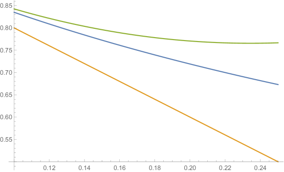
Figure 2: The ratio $R(b\equiv\frac{32}{m_{H}})$ (blue) compared with its first order (yellow) and second order (green) Taylor expansion. At $\frac{1}{m_{H}}=\frac{1}{4}$ one has $R(b)\approx 0.67$, while at $\frac{1}{m_{H}}=\frac{1}{10}$ one has $R(b)\approx 0.84$. As $b\rightarrow\infty$, $R(b)\rightarrow 0$. At $\frac{1}{m_{H}}=\frac{1}{4}$ the second order result is about $10\%$ larger than of the full result.

Appendix C Details of the heavy pentaquark masses

Here we detail the various contributions to the mass spectra recorded in Table 1 and Table 2. For completeness, we recall that we fix $M_{D}=1.87$ GeV to reproduce the D-meson mass in (9) and fix $M_{KK}=0.475$ GeV to reproduce the $M_{\Lambda_{c}}=2.286$ GeV. As result, we have for the charmed heavy-light hadrons recorded in Table 1

$$M_{\Lambda_{c}}=m_{H}+m_{N}-0.82M_{KK}+0.253\frac{M_{KK}^{2}}{m_{H}}=2.286{\text{G}eV}\ ,$$ (127)

$$M_{\Sigma_{c}}(\frac{1}{2})=m_{H}+m_{N}-0.234M_{KK}+0.203\frac{M_{KK}^{2}}{m_{H}}=2.557{\text{G}eV}\ ,$$ (128)

$$M_{\Sigma_{c}}(\frac{3}{2})=m_{H}+m_{N}-0.154M_{KK}+0.203\frac{M_{KK}^{2}}{m_{H}}=2.596{\text{G}eV}\ ,$$ (129)

$$M_{\Lambda_{c}^{\star}}(P=-1)=m_{H}+m_{N}-0.82M_{KK}+\frac{2}{\sqrt{6}}M_{KK}+0.321\frac{M_{KK}^{2}}{m_{H}}=2.683{\text{G}eV}\ ,$$ (130)

$$M_{\Lambda_{c}^{\star}}(P=1)=m_{H}+m_{N}+0.107M_{KK}+0.253\frac{M_{KK}^{2}}{m_{H}}=2.726{\text{G}eV}\ ,$$ (131)

$$P_{c}(J=\frac{1}{2},S=0)=2m_{H}+m_{N}-0.078M_{KK}+0.404\frac{M_{KK}^{2}}{m_{H}}=4.360{\text{G}eV}\ ,$$ (132)

$$P_{c}(J=\frac{1}{2},S=1)=2m_{H}+m_{N}-0.119M_{KK}+0.404\frac{M_{KK}^{2}}{m_{H}}=4.341{\text{G}eV}\ ,$$ (133)

$$P_{c}(J=\frac{3}{2},S=1)=2m_{H}+m_{N}-0.05M_{KK}+0.404\frac{M_{KK}^{2}}{m_{H}}=4.373{\text{G}eV}\ .$$ (134)

For the bottom heavy-light hadrons we fix the heavy-light meson mass $m_{H}=(5.28-0.168)$ GeV=$10.76M_{KK}$. The bottom heavy-light mass spectra recorded in Table 2 follow from

$$M_{\Lambda_{b}}=m_{H}+m_{N}-0.958M_{KK}+0.253\frac{M_{KK}^{2}}{m_{H}}=5.608{\text{G}eV}\ ,$$ (135)

$$M_{\Sigma_{b}}(\frac{1}{2})=m_{H}+m_{N}-0.207M_{KK}+0.203\frac{M_{KK}^{2}}{m_{H}}=5.962{\text{G}eV}\ ,$$ (136)

$$M_{\Sigma_{b}}(\frac{3}{2})=m_{H}+m_{N}-0.174M_{KK}+0.203\frac{M_{KK}^{2}}{m_{H}}=5.978{\text{G}eV}\ ,$$ (137)

$$M_{\Lambda_{b}^{\star}}(P=-1)=m_{H}+m_{N}-0.958M_{KK}+\frac{2}{\sqrt{6}}M_{KK}+0.321\frac{M_{KK}^{2}}{m_{H}}=5.998{\text{G}eV}\ ,$$ (138)

$$M_{\Lambda_{b}}^{\star}(P=1)=m_{H}+m_{N}-0.072M_{KK}+0.253\frac{M_{KK}^{2}}{m_{H}}=6.029{\text{G}eV}\ ,$$ (139)

$$P_{b}(J=\frac{1}{2},S=0)=2m_{H}+m_{N}-0.0393M_{KK}+0.404\frac{M_{KK}^{2}}{m_{H}}=11.163{\text{G}eV}\ ,$$ (140)

$$P_{b}(J=\frac{1}{2},S=1)=2m_{H}+m_{N}-0.056M_{KK}+0.404\frac{M_{KK}^{2}}{m_{H}}=11.155{\text{G}eV}\ ,$$ (141)

$$P_{b}(J=\frac{3}{2},S=1)=2m_{H}+m_{N}-0.030M_{KK}+0.404\frac{M_{KK}^{2}}{m_{H}}=11.196{\text{G}eV}\ .$$ (142)

References

- Aaij et al. (2019) Roel Aaij et al. (LHCb), “Observation of a narrow pentaquark state, , and of two-peak structure of the ,” Phys. Rev. Lett. 122, 222001 (2019), arXiv:1904.03947 [hep-ex] .
- Aaij et al. (2015) Roel Aaij et al. (LHCb), “Observation of Resonances Consistent with Pentaquark States in Decays,” Phys. Rev. Lett. 115, 072001 (2015), arXiv:1507.03414 [hep-ex] .
- Liu and Zahed (2017a) Yizhuang Liu and Ismail Zahed, “Heavy Baryons and their Exotics from Instantons in Holographic QCD,” Phys. Rev. D 95, 116012 (2017a), arXiv:1704.03412 [hep-ph] .
- Wu et al. (2010) Jia-Jun Wu, R. Molina, E. Oset, and B. S. Zou, “Prediction of narrow and resonances with hidden charm above 4 GeV,” Phys. Rev. Lett. 105, 232001 (2010), arXiv:1007.0573 [nucl-th] .
- Karliner and Rosner (2015) Marek Karliner and Jonathan L. Rosner, “New Exotic Meson and Baryon Resonances from Doubly-Heavy Hadronic Molecules,” Phys. Rev. Lett. 115, 122001 (2015), arXiv:1506.06386 [hep-ph] .
- Burns (2015) T. J. Burns, “Phenomenology of Pc(4380)+, Pc(4450)+ and related states,” Eur. Phys. J. A 51, 152 (2015), arXiv:1509.02460 [hep-ph] .
- Richard (2016) Jean-Marc Richard, “Exotic hadrons: review and perspectives,” Few Body Syst. 57, 1185–1212 (2016), arXiv:1606.08593 [hep-ph] .
- Lebed et al. (2017) Richard F. Lebed, Ryan E. Mitchell, and Eric S. Swanson, “Heavy-Quark QCD Exotica,” Prog. Part. Nucl. Phys. 93, 143–194 (2017), arXiv:1610.04528 [hep-ph] .
- Esposito et al. (2017) A. Esposito, A. Pilloni, and A. D. Polosa, “Multiquark Resonances,” Phys. Rept. 668, 1–97 (2017), arXiv:1611.07920 [hep-ph] .
- Olsen et al. (2018) Stephen Lars Olsen, Tomasz Skwarnicki, and Daria Zieminska, “Nonstandard heavy mesons and baryons: Experimental evidence,” Rev. Mod. Phys. 90, 015003 (2018), arXiv:1708.04012 [hep-ph] .
- Guo et al. (2018) Feng-Kun Guo, Christoph Hanhart, Ulf-G. Meißner, Qian Wang, Qiang Zhao, and Bing-Song Zou, “Hadronic molecules,” Rev. Mod. Phys. 90, 015004 (2018), arXiv:1705.00141 [hep-ph] .
- Karliner et al. (2018) Marek Karliner, Jonathan L. Rosner, and Tomasz Skwarnicki, “Multiquark States,” Ann. Rev. Nucl. Part. Sci. 68, 17–44 (2018), arXiv:1711.10626 [hep-ph] .
- Maiani et al. (2015) L. Maiani, A. D. Polosa, and V. Riquer, “The New Pentaquarks in the Diquark Model,” Phys. Lett. B 749, 289–291 (2015), arXiv:1507.04980 [hep-ph] .
- Lebed (2015) Richard F. Lebed, “The Pentaquark Candidates in the Dynamical Diquark Picture,” Phys. Lett. B 749, 454–457 (2015), arXiv:1507.05867 [hep-ph] .
- Eides et al. (2020) Michael I. Eides, Victor Yu Petrov, and Maxim V. Polyakov, “New LHCb pentaquarks as hadrocharmonium states,” Mod. Phys. Lett. A 35, 2050151 (2020), arXiv:1904.11616 [hep-ph] .
- Du et al. (2021) Meng-Lin Du, Vadim Baru, Feng-Kun Guo, Christoph Hanhart, Ulf-G. Meißner, José A. Oller, and Qian Wang, “Revisiting the nature of the pentaquarks,” (2021), arXiv:2102.07159 [hep-ph] .
- Shuryak (1982) Edward V. Shuryak, “Hadrons Containing a Heavy Quark and QCD Sum Rules,” Nucl. Phys. B 198, 83–101 (1982).
- Isgur and Wise (1991) Nathan Isgur and Mark B. Wise, “Spectroscopy with heavy quark symmetry,” Phys. Rev. Lett. 66, 1130–1133 (1991).
- Nowak et al. (1993) Maciej A. Nowak, Mannque Rho, and I. Zahed, “Chiral effective action with heavy quark symmetry,” Phys. Rev. D 48, 4370–4374 (1993), arXiv:hep-ph/9209272 .
- Bardeen and Hill (1994) William A. Bardeen and Christopher T. Hill, “Chiral dynamics and heavy quark symmetry in a solvable toy field theoretic model,” Phys. Rev. D 49, 409–425 (1994), arXiv:hep-ph/9304265 .
- Nowak et al. (2004) Maciej A. Nowak, Michal Praszalowicz, Mariusz Sadzikowski, and Joanna Wasiluk, “Chiral doublers of heavy light baryons,” Phys. Rev. D 70, 031503 (2004), arXiv:hep-ph/0403184 .
- Aubert et al. (2003) B. Aubert et al. (BaBar), “Observation of a narrow meson decaying to at a mass of 2.32-GeV/c2,” Phys. Rev. Lett. 90, 242001 (2003), arXiv:hep-ex/0304021 .
- Besson et al. (2003) D. Besson et al. (CLEO), “Observation of a narrow resonance of mass 2.46-GeV/c**2 decaying to D*+(s) pi0 and confirmation of the D*(sJ)(2317) state,” Phys. Rev. D 68, 032002 (2003), [Erratum: Phys.Rev.D 75, 119908 (2007)], arXiv:hep-ex/0305100 .
- Maldacena (1999) Juan Martin Maldacena, “The Large N limit of superconformal field theories and supergravity,” Int. J. Theor. Phys. 38, 1113–1133 (1999), arXiv:hep-th/9711200 .
- Erlich et al. (2005) Joshua Erlich, Emanuel Katz, Dam T. Son, and Mikhail A. Stephanov, “QCD and a holographic model of hadrons,” Phys. Rev. Lett. 95, 261602 (2005), arXiv:hep-ph/0501128 .
- Sakai and Sugimoto (2005) Tadakatsu Sakai and Shigeki Sugimoto, “Low energy hadron physics in holographic QCD,” Prog. Theor. Phys. 113, 843–882 (2005), arXiv:hep-th/0412141 .
- Fujiwara et al. (1985) Takanori Fujiwara, Taichiro Kugo, Haruhiko Terao, Shozo Uehara, and Koichi Yamawaki, “Nonabelian Anomaly and Vector Mesons as Dynamical Gauge Bosons of Hidden Local Symmetries,” Prog. Theor. Phys. 73, 926 (1985).
- Liu and Zahed (2017b) Yizhuang Liu and Ismail Zahed, “Holographic Heavy-Light Chiral Effective Action,” Phys. Rev. D 95, 056022 (2017b), arXiv:1611.03757 [hep-ph] .
- Liu and Zahed (2017c) Yizhuang Liu and Ismail Zahed, “Heavy and Strange Holographic Baryons,” Phys. Rev. D 96, 056027 (2017c), arXiv:1705.01397 [hep-ph] .
- Li (2017) Si-wen Li, “Holographic heavy-baryons in the Witten-Sakai-Sugimoto model with the D0-D4 background,” Phys. Rev. D 96, 106018 (2017), arXiv:1707.06439 [hep-th] .
- Fujii and Hosaka (2020) Daisuke Fujii and Atsushi Hosaka, “Heavy baryons in holographic QCD with higher dimensional degrees of freedom,” Phys. Rev. D 101, 126008 (2020), arXiv:2003.13415 [hep-ph] .
- Hata et al. (2007) Hiroyuki Hata, Tadakatsu Sakai, Shigeki Sugimoto, and Shinichiro Yamato, “Baryons from instantons in holographic QCD,” Prog. Theor. Phys. 117, 1157 (2007), arXiv:hep-th/0701280 .
- Hashimoto et al. (2008) Koji Hashimoto, Tadakatsu Sakai, and Shigeki Sugimoto, “Holographic Baryons: Static Properties and Form Factors from Gauge/String Duality,” Prog. Theor. Phys. 120, 1093–1137 (2008), arXiv:0806.3122 [hep-th] .
- Kim and Zahed (2008) Keun-Young Kim and Ismail Zahed, “Electromagnetic Baryon Form Factors from Holographic QCD,” JHEP 09, 007 (2008), arXiv:0807.0033 [hep-th] .
- Hata and Murata (2008) Hiroyuki Hata and Masaki Murata, “Baryons and the Chern-Simons term in holographic QCD with three flavors,” Prog. Theor. Phys. 119, 461–490 (2008), arXiv:0710.2579 [hep-th] .
- Hashimoto et al. (2010) Koji Hashimoto, Norihiro Iizuka, Takaaki Ishii, and Daisuke Kadoh, “Three-flavor quark mass dependence of baryon spectra in holographic QCD,” Phys. Lett. B 691, 65–71 (2010), arXiv:0910.1179 [hep-th] .
- Lau and Sugimoto (2017) Pak Hang Chris Lau and Shigeki Sugimoto, “Chern-Simons five-form and holographic baryons,” Phys. Rev. D 95, 126007 (2017), arXiv:1612.09503 [hep-th] .
- Zahed and Brown (1986) I. Zahed and G. E. Brown, “The Skyrme Model,” Phys. Rept. 142, 1–102 (1986).
- Rho et al. (1992) Mannque Rho, D. O. Riska, and N. N. Scoccola, “The Energy levels of the heavy flavor baryons in the topological soliton model,” Z. Phys. A 341, 343–352 (1992).
- Rho and Zahed (2017) Mannque Rho and Ismail Zahed, “Multifaceted Skyrmion,” (2017).
- Lin and Zou (2019) Yong-Hui Lin and Bing-Song Zou, “Strong decays of the latest LHCb pentaquark candidates in hadronic molecule pictures,” Phys. Rev. D 100, 056005 (2019), arXiv:1908.05309 [hep-ph] .
- Dosch et al. (2015) Hans Gunter Dosch, Guy F. de Teramond, and Stanley J. Brodsky, “Supersymmetry Across the Light and Heavy-Light Hadronic Spectrum,” Phys. Rev. D 92, 074010 (2015), arXiv:1504.05112 [hep-ph] .
- Sonnenschein and Weissman (2019) Jacob Sonnenschein and Dorin Weissman, “Excited mesons, baryons, glueballs and tetraquarks: Predictions of the Holography Inspired Stringy Hadron model,” Eur. Phys. J. C 79, 326 (2019), arXiv:1812.01619 [hep-ph] .