Birth of the ELMs: a ZTF survey for evolved cataclysmic variables turning into extremely low-mass white dwarfs

Abstract

We present a systematic survey for mass-transferring and recently-detached cataclysmic variables (CVs) with evolved secondaries, which are progenitors of extremely low mass white dwarfs (ELM WDs), AM CVn systems, and detached ultracompact binaries. We select targets below the main sequence in the Gaia color-magnitude diagram with ZTF light curves showing large-amplitude ellipsoidal variability and orbital period $P_{\rm orb}<6$ hr. This yields 51 candidates brighter than $G=18$, of which we have obtained many-epoch spectra for 21. We confirm all 21 to be completely– or nearly–Roche lobe filling close binaries. 13 show evidence of ongoing mass transfer, which has likely just ceased in the other 8. Most of the secondaries are hotter than any previously known CV donors, with temperatures $4700<T_{{\rm eff}}/{\rm K}<8000$. Remarkably, all secondaries with $T_{\rm eff}\gtrsim 7000\,\rm K$ appear to be detached, while all cooler secondaries are still mass-transferring. This transition likely marks the temperature where magnetic braking becomes inefficient due to loss of the donor’s convective envelope. Most of the proto-WD secondaries have masses near $0.15\,M_{\odot}$; their companions have masses near $0.8\,M_{\odot}$. We infer a space density of $\sim 60\,\rm kpc^{-3}$, roughly 80 times lower than that of normal CVs and three times lower than that of ELM WDs. The implied Galactic birth rate, $\mathcal{R}\sim 60\,\rm Myr^{-1}$, is half that of AM CVn binaries. Most systems are well-described by MESA models for CVs in which mass transfer begins only as the donor leaves the main sequence. All are predicted to reach minimum periods $5\lesssim P_{{\rm orb}}/{\rm min}\lesssim 30$ within a Hubble time, where they will become AM CVn binaries or merge. This sample triples the known evolved CV population and offers broad opportunities for improving understanding of the compact binary population.

1 Introduction

Cataclysmic variables (CVs) are short-period binaries in which a low-mass star transfers mass to a white dwarf (WD) through stable Roche lobe overflow (RLOF; see Warner, 2003, for a review). At orbital periods $P_{\rm orb}\lesssim 6$ hours, the mass-losing stars in most CVs fall on a tight “donor sequence” of mass, radius, spectral type, and luminosity as a function of period (Patterson, 1984; Beuermann et al., 1998; Smith & Dhillon, 1998; Knigge, 2006; Knigge et al., 2011; Abrahams et al., 2020). This sequence, and the distribution of CV periods along it, has proved foundational for the development and testing of models for mass transfer in interacting binaries.

By definition, the donor stars in CVs have radii equal to their Roche lobe radii. This imposes a (nearly) deterministic relation between the orbital period, $P_{\rm orb}$, and the donor’s mean density, $\overline{\rho}_{\rm donor}$:

$$\overline{\rho}_{\rm donor}\approx 107\,{\rm g\,cm^{-3}}\left(P_{\rm orb}/{\rm hr}\right)^{-2},$$ (1)

with very weak dependence on the mass of either component. Here $\overline{\rho}_{\rm donor}=3M_{\rm donor}/\left(4\pi R_{\rm donor}^{3}\right)$, with $M_{\rm donor}$ and $R_{\rm donor}$ the mass and equivalent radius of the mass-losing star. Most CV donors are only mildly out of thermal equilibrium due to mass loss, so their radii and effective temperatures differ only modestly from those of single main sequence stars of the same mass (Knigge, 2006). The long-term evolution of CVs is governed foremost by angular momentum loss through magnetic braking and gravitational radiation, which shrink the orbits of CVs and in turn reduce the mass of the donors. The CV donor sequence is thus an evolutionary track, with initially massive donors in longer-period CVs evolving along the sequence to short periods and low masses.

A small fraction of CV donors are observed to deviate significantly from the donor sequence, with unusually high effective temperatures and luminosities for their orbital period (e.g. Thorstensen et al., 2002b, a). These objects are rare compared to normal CVs, but about a dozen have been identified over the last two decades, mostly with K-type donor stars ($T_{\rm eff}\approx 4,500\,\rm K$, at periods where ordinary CV donors have $T_{\rm eff}\lesssim 3,500\,\rm K$). A particularly extreme member of this evolved CV population is the recently discovered binary LAMOST J0140, with an F-type donor at a period of 3.81 hours (El-Badry et al., 2021b).

Such overluminous donors are thought to form from CVs in which the donor’s first Roche lobe overflow only occurs near the end of its main-sequence evolution, as it is beginning to form a helium core. By the time they reach short periods, these “evolved CV” donors are predicted to consist of a helium core with a thick (few hundredths of a solar mass) hydrogen envelope, whose luminosity comes primarily from hydrogen shell burning. Their expected mass transfer rates are much lower than in normal CVs of similar period, and the donor effective temperatures are higher. Eventually, the most evolved donors are expected to detach from their Roche lobes, contracting and heating at near constant luminosity, until they become extremely low-mass (ELM) white dwarfs (e.g. Sun & Arras, 2018). The timescale for this contraction and evolution toward the WD cooling track is set by the remaining mass of burnable hydrogen in the envelope of the proto-ELM WD and is typically about a Gyr (e.g. Istrate et al., 2014).

The formation and evolution of such detached ELM WDs – which have attracted attention as companions to millisecond pulsars (e.g. Driebe et al., 1998), progenitors of ultracompact binaries (e.g. Tutukov et al., 1985, 1987; Podsiadlowski et al., 2003) and thermonuclear supernovae (e.g. Livne, 1990; Bildsten et al., 2007), and as some of the loudest gravitational wave sources in the LISA band (e.g. Hermes et al., 2012; Kupfer et al., 2018) – has been an area of active study in the last decade. Much of what is known observationally about the ELM WD population is due to the ELM survey (Brown et al., 2010), which carried out targeted spectroscopic follow-up of ELM candidates based on SDSS colors. The survey’s final sample (Brown et al., 2020) contained 98 spectroscopically vetted double white dwarf binaries, including 79 in which at least one component has an inferred mass below $0.3\,M_{\odot}$. Essentially all ELM WDs appear to be in short-period binaries. Those discovered by the ELM survey have periods ranging from 0.0089 to 1.5 days, with a median period of 0.25 days. All of their companions are consistent with being other WDs, though some could also be neutron stars.

The objects detected by the ELM survey all have effective temperatures $T_{\rm eff}>8000\,\rm K$, and most have surface gravities $\log\left[g/\left({\rm cm\,s^{-2}}\right)\right]>5.5$. This is largely a consequence of the color selection the survey employed. Cooler and more bloated ELM WDs – objects that were until recently CVs with ongoing mass transfer – are expected to exist. However, their temperatures and surface gravities are predicted to be similar to those of main sequence A and F stars, so they are not easily identified with color cuts alone (e.g. Pelisoli et al., 2018).

This paper introduces a systematic search for these cooler and more bloated ELM WDs, and the evolved CVs from which they formed. Although their colors are usually indistinguishable from those of main sequence stars, their smaller masses and radii cause them to fall below the main sequence. Periodic light curve variability due to tidal distortion allows us to distinguish them from low-metallicity main-sequence stars, which inhabit a similar region of the color-magnitude diagram. Throughout the paper, we refer to such nascent ELM WDs and unusually warm CV donors as “proto-WDs” and “evolved CV donors” interchangeably: we are interested in both objects with ongoing mass transfer and those that have recently terminated mass transfer.

The remainder of this paper is organized as follows. Section 2 describes our selection of proto-ELM WD candidates, which is based on CMD position and ellipsoidal light curve variability. Section 3 describes our follow-up spectroscopic observations and modeling to constrain system masses, radii, and luminosities. In most cases, joint modeling of light curves, spectra, radial velocities, parallaxes, and broadband spectral energy distributions allows us to obtain precise constraints on the masses and radii of the donor stars, and somewhat weaker constraints on the companion masses. Section 4 compares the inferred physical parameters of the binaries in our sample to those of objects from other surveys and to binary evolution models. We discuss our survey’s selection function and the space density of evolved CVs and proto-ELM WDs in Section 5, and we summarize our findings in Section 6.

The Appendices provide additional details. Appendix A describes the priors adopted in our inference of donor masses and radii. Appendix B shows the H$\alpha$ line profiles of objects in our sample. Appendix C explores the long-term brightness evolution and sources of photometric scatter in the observed light curves. Appendix D presents objects in the light curve-selected sample for which we have not yet obtained spectroscopic follow-up. Appendix E explores the overlap of our sample with other surveys.

2 Sample selection

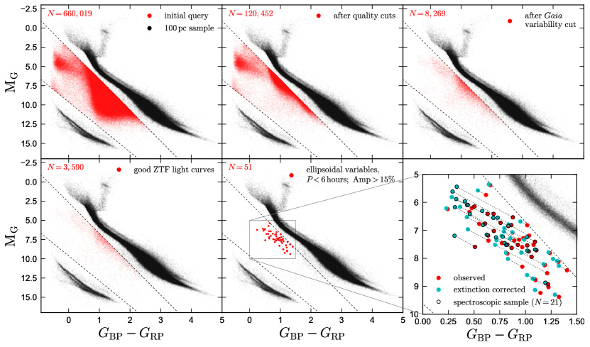
Figure 1: Sample selection in the color-magnitude diagram. In all panels, black points show the Gaia 100 pc sample for context. Red points show our candidates (not limited to 100 pc) at various stages of cleaning. We first (upper left) select all sources with precise parallaxes that fall between the main sequence and WD cooing sequence. Many of these sources have spurious parallaxes or colors; we apply astrometric and photometric quality cuts to remove these (upper middle). We then require significant scan-to-scan brightness variability as estimated from the Gaia flux RMS (upper right), and that sources have a good ZTF light curve (bottom left). Finally, we inspect the ZTF light curves individually and select objects dominated by ellipsoidal variability with $P_{\rm orb}<6$ hours. Bottom right panel shows the final sample with (cyan) and without (red) an extinction/reddening correction. Objects for which we have obtained spectroscopic follow-up are marked with a border.

The objects we hope to find have similar temperatures and surface gravities to main sequence AFGK stars, but with lower masses and smaller radii. They are thus expected to fall below the main sequence in the color–absolute magnitude diagram (CMD). Normal CVs with unevolved donors also fall in this region of the CMD (e.g. Abril et al., 2020; Abrahams et al., 2020) – not because their donors are below the main sequence, but because a disk around the accreting WD dominates the optical photometry. To filter out normal CVs, we target objects whose optical light curves are dominated by ellipsoidal variability of the donor star (e.g. Wilson & Sofia, 1976), induced by tidal distortion from the companion. At short periods ($P_{\rm orb}<6$ hours), this is only expected to occur if the donor is warmer and more luminous than in a normal CV (e.g. Rebassa-Mansergas et al., 2014; Wakamatsu et al., 2021). Our spectroscopic follow-up (Section 3) demonstrates that this approach efficiently eliminates normal CVs and other evolved-CV imposters, such as detached main sequence + WD binaries and metal-poor main sequence stars that naturally fall below the main sequence.

2.1 Gaia CMD selection

We began by selecting from Gaia eDR3 (Gaia Collaboration et al., 2021a) relatively bright sources ($G<18$) with precise parallaxes ($\varpi/\sigma_{\varpi}>5$) that fall between the main sequence and WD cooling sequence in the color-magnitude diagram. This was accomplished with the following ADQL query,

⬇

select * from gaiaedr3.gaia_source

where parallax_over_error > 5

and phot_g_mean_mag < 18

and phot_g_mean_mag + 5 * log10(parallax / 100) < (3.25*bp_rp + 9.625)

and phot_g_mean_mag + 5 * log10(parallax / 100) > (4*bp_rp + 2.7)

and phot_rp_mean_flux_over_error > 5

and phot_bp_mean_flux_over_error > 5

and astrometric_sigma5d_max < 1

which returned 660,019 sources. These are plotted in the upper left panel of Figure 1, where for context we also plot a clean sample of Gaia sources within 100 pc (Gaia Collaboration et al., 2021b). The photometry and astrometry of the 100 pc sample has higher SNR and is cleaner (i.e., subject to more quality cuts) than a large majority of sources returned by our query. It is also limited to a smaller volume, and thus is less biased toward intrinsically bright sources.

A large fraction of sources between the main sequence and WD cooling sequence – a region of the CMD which, astrophysically, is expected to be sparsely populated – are spurious. A tiny fraction of normal main sequence stars being scattered into this region may thus dominate the initial selection. We applied several quality cuts to minimize contamination from sources with unreliable parallaxes and/or colors. Within the initial query, the requirement of astrometric_sigma5d_max < 1 removes sources for which a good astrometric fit could not be achieved with a single-star astrometric model (see Fabricius et al., 2021; Gaia Collaboration et al., 2021b), and the cuts of phot_bp/rp_mean_flux_over_error > 5 ensure that the colors are not too noisy.

To further reduce the number of sources with spurious astrometric solutions, we retrieved the astrometric fidelity parameter calculated by Rybizki et al. (2021, “fidelity_v1”) for all sources returned by the initial query. This parameter is calculated based on 14 quantities reported in Gaia eDR3 using a neural network classifier that is trained on sources with both high-quality and manifestly incorrect parallaxes. We remove all sources for which fidelity_v1 < 0.75, corresponding approximately to a $<25\%$ probability of a spurious astrometric solution. This left us with 161,614 sources.

Besides having spurious astrometry, sources can also appear below the main sequence if they have unreliable colors. Gaia colors are calculated by integrating over low-resolution spectra that are dispersed over a $3.5\times 2.1$ arcsec data acquisition window; they are therefore quite susceptible to blending by nearby sources. Various photometric flags are provided as part of Gaia eDR3 to identify sources with unreliable colors (Evans et al., 2018; Riello et al., 2021), but these also remove some sources in sparse regions of the sky with apparently good photometry. After some experimentation, we opted to remove all sources that have a companion within 6 arcsec with brighter $G$-band magnitude than the source itself. This removed an additional 41,162 sources, leaving us with 120,452 sources (upper middle panel of Figure 1). We verified that both this cut and the astrometric fidelity cut remove only a small fraction ($\sim 5\%$) of sources with reliable astrometry and photometry as judged by their CMD position (i.e., sources on the main sequence). We can thus safely use them to eliminate “junk” without seriously affecting the selection function of our search (e.g. Rix et al., 2021).

We next wish to identify ellipsoidal variables. Before querying light curves for all sources, we applied a crude cut to filter out most non-variable sources using Gaia variability flags. Photometrically variable sources can be identified based on the flux “error” reported in the Gaia archive, which is calculated empirically from the scatter in flux measurements across multiple scans. Following Guidry et al. (2021), we calculate a $G$-band variability metric,

$$V_{G}=\frac{\sigma_{F}}{\left\langle F\right\rangle}\sqrt{n_{{\rm obs}}},$$ (2)

where $\sigma_{F}$, $\left\langle F\right\rangle$, and $n_{{\rm obs}}$ refer respectively to the parameters phot_g_mean_flux_error, phot_g_mean_flux, and phot_g_n_obs in the Gaia archive. Not all scan-to-scan flux variability is astrophysical: for faint sources, scatter due to photon noise is significant. We therefore compute a modified variability metric,

$$\tilde{V}_{G}=V_{G}-f\left(G\right),$$ (3)

where $f(G)$ is a fitting function taken from Guidry et al. (2021, their Equation E1) that approximately represents the 99th percentile of $V_{G}$ at a given $G$ magnitude. We only retain sources with $\tilde{V}_{G}>0.02$. This cuts the sample to 8,269 sources, which are shown in the upper right panel of Figure 1.

2.2 Light curve selection

We next searched for ellipsoidal variables among these candidates. Of the 8,269 remaining sources, 4,819 have declination $\delta>-28$ deg, such that they could potentially fall within the footprint of the Zwicky Transient Facility (ZTF; Bellm et al., 2019; Graham et al., 2019; Masci et al., 2019). We queried the public ZTF 4th data release, which was the most recent release at the time of our sample selection, for $g-$ and $r-$ band light curves of all these sources. This yielded light curves for 4,066 objects. Investigating the 753 sources that did not have light curves, we found that a majority of them are faint stars that are close (6-15 arcsec) to a very bright star ($G\lesssim 9$). We have no reason to expect genuine CVs or ELM WDs to be preferentially found in such a configuration, so we suspect that these are simply sources with blended Gaia photometry that are not really below the main sequence.

In order to be able to reliably identify periodicity, we only considered sources for which the ZTF DR4 light curves contained at least 40 clean visits in at least one bandpass. This left us with 3,590 sources (bottom left panel of Figure 1).

We inspected the ZTF light curves of these sources individually. About half show clear evidence of variability, with uncertainty-normalized RMS variability greater than 1.5 (where the expected value for a non-variable source is $\approx 1$). The fact that a significant number of apparently non-variable sources enter the sample reflects the fact that the Gaia flux errors are an imperfect proxy for variability. We find that increasing the $\tilde{V}_{G}$ threshold can significantly reduce the number of non-variable sources that enter the sample, but at the expense of completeness for true variable sources.

To find periodic variables, we computed Lomb–Scargle periodograms (e.g. VanderPlas, 2018) on a period grid from 1 to 24 hours. We visually inspected the periodograms as well as the effects of folding the light curves to the 6 most significant periods. Many CVs and related objects are known to exhibit quasi-regular outbursts (“dwarf novae”) due to disk instability (e.g. Hameury, 2020). To reduce the chance of such outbursts confounding our period search, we also removed the brightest 5% of points in each light curve and inspected periodograms computed from the remaining photometric points.

The search revealed a menagerie of light curve types, of which a few examples are shown in Figure 2. Many sources show irregular variability on a range of timescales, characteristic of CVs and nova-like variables (see Szkody et al., 2020, for a study of CVs with ZTF). Other sources show deep, boxy eclipses; in this region of the CMD, these are mainly detached WD + main sequence binaries in which the WD is hot (e.g. Parsons et al., 2010). Ellipsoidal variables – what we are searching for – show approximately sinusoidal variability but with brightness minima of alternating depths due to gravity darkening (see Figure 3). Non-eclipsing binaries containing a WD or hot subdwarf and a cool, main-sequence companion often show a quasi-sinusoidal reflection effect (e.g. Ratzloff et al., 2020). These light curves appear similar to ellipsoidal variables but lack the alternating minima caused by gravity darkening. We find many such systems with $\rm M_{G}\lesssim 5$ and very blue colors; these likely contain hot subdwarfs (stripped core He-burning stars) rather than WDs. Among these are both pure reflection systems and “HW Vir”-type systems showing eclipses (e.g. Schaffenroth et al., 2019; Enenstein et al., 2021).

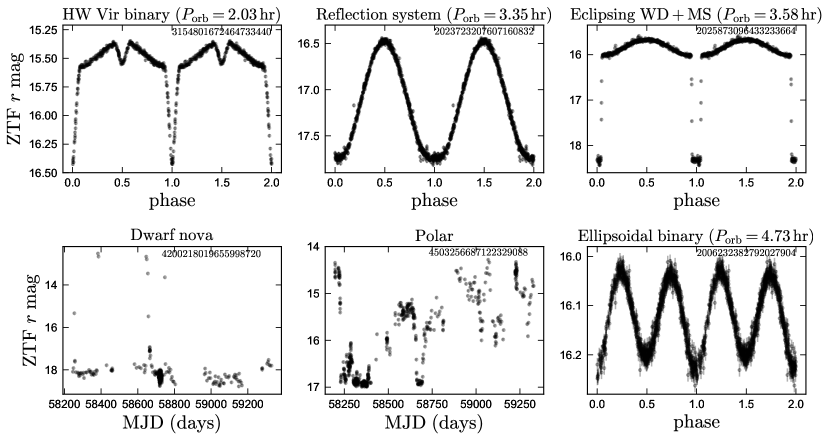
Figure 2: Examples of various classes of variables found between the main sequence and WD cooling track in the CMD (lower left panel of Figure 1). Upper left: HW Vir type binary, in which an M dwarf orbits a core helium burning hot subdwarf nearly edge-on. Upper center: reflection effect binary, in which an M dwarf orbits a hot white dwarf and is heated on one side. Upper right: eclipsing white dwarf + main sequence binary, also displaying a reflection effect. Bottom left: dwarf nova (CV) displaying outbursts and other variability due to changes in disk structure. Bottom center: polar (i.e., a magnetic CV) displaying irregular variability on a range of timescales. Bottom right: ellipsoidal variable, our primary targets of interest. These can be distinguished from reflection systems by their unequal light curve minima. All objects are labeled by their Gaia eDR3 IDs.

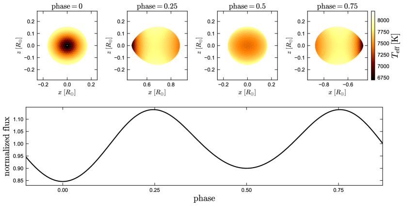
Figure 3: Schematic illustration of ellipsoidal variability using a Phoebe model for a Roche-filling star with similar parameters to objects in our sample. The geometric cross-section of the tidally-distorted donor is larger when it is viewed edge-on (phase 0.25 and 0.75) than when it is viewed end-on (phase 0 or 0.5). This gives rise to quasi-sinusoidal variability with maximum power at half the orbital period. Regions of the photosphere with lower surface gravity are cooler than higher-gravity regions; this “gravity darkening” gives rise to unequal light curve minima. The maximum peak-to-peak amplitude expected for pure ellipsoidal variation is about 30%, with some dependence on the gravity- and limb-darkening law.

To isolate sources likely to be evolved CVs and recently detached proto-ELM WDs, we searched specifically for sources meeting the following criteria:

1. Evidence of ellipsoidal variability, with brightness minima of alternating depths (Figure 3). This ensures that the donor star, not an accretion disk, dominates the optical light curve, and thus selects systems with overluminous donors and/or underluminous disks. We do not insist that light curves shown only ellipsoidal variability. Some of our targets also show evidence of eclipses (likely from an accretion disk around a WD companion), long-term brightness evolution, and other scatter not captured by a pure ellipsoidal model.

2. Orbital periods $P_{\rm orb}<6$ hours. This limit is chosen to allow us to straightforwardly distinguish CVs with the most evolved donors from “normal” CVs, since it is only at $P_{\rm orb}\lesssim 6$ hours that most CV donors fall on a tight and well-defined donor sequence (see Knigge 2006; at longer periods, all donors are evolved). This limit also ensures that both stars are relatively small, and (in most cases) evolved, because binaries containing two main-sequence stars with orbital periods shorter than 5 hours are very rare (e.g. Rucinski, 2007; Jayasinghe et al., 2020). This prevents, e.g., main-sequence contact binaries with spurious colors or parallaxes from entering the sample.

3. Peak-to-peak variability amplitude greater than 15% in the $g-$band. This selects binaries in which the tidally distorted star is nearly or completely Roche-lobe filling (Section 3.6); in practice, it corresponds to a filling factor $R_{\rm donor}/R_{\rm Roche\,lobe}\gtrsim 0.8$.

4. Similar variability amplitude in the $g$ and $r$ bands (within $20\%$). This excludes most systems in which a significant fraction of the optical light is contributed by a disk or by a hot WD companion; such systems have more dilution, and thus lower variability amplitude, in the $g$ band.

5. Not a hot subdwarf: we excluded a few ellipsoidal systems in the hot-subdwarf clump of the CMD, with $M_{G}<5$ and $G_{\rm BP}-G_{\rm RP}<0.2$. Such systems are likely binaries containing a WD and a core helium burning star, with different evolutionary histories from the objects we seek.

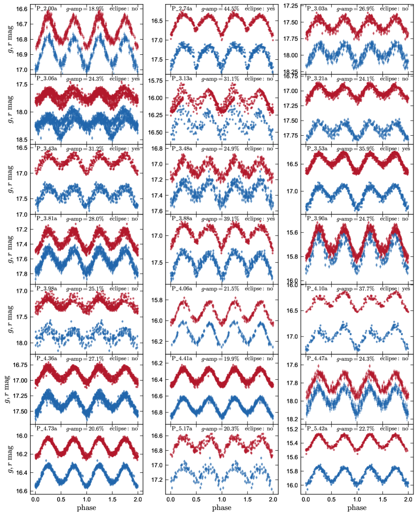
Figure 4: Phased ZTF $g$ (blue) and $r$ (red) light curves for all targets in the spectroscopic sample. Targets are sorted by increasing orbital period. A diversity of light curve morphologies is evident. Some targets have light curves suggestive of ellipsoidal a variation with little intrinsic scatter (e.g. P_2.00a). Others show evidence of eclipses (e.g. P_2.74a). A majority show significant intrinsic scatter (e.g. P_3.03a).

Given our selection criteria, the most common false-positives with similar light curve shapes to ellipsoidal variables are non-eclipsing reflection effect binaries consisting of a hot, compact star and a cooler companion (typically an M dwarf). These can be distinguished from ellipsoidal variables because (a) their variability amplitudes are significantly larger in the $r$-band than in the $g$-band, and (b) they lack the unequal minima of ellipsoidal variables. Some single-mode pulsators also have light curve shapes similar to ellipsoidal variables, but these also lack unequal minima.

2.3 Final sample

Table 1: Basic properties of sources in the spectroscopic sample. “ID” (internal to this work) is based on orbital period in hours; we also list Gaia eDR3 IDs. $l$ and $b$ are Galactic longitude and latitude. $G$ is the Gaia mean magnitude. $P_{\rm orb}$ is the spectroscopically-confirmed orbital period. $\varpi_{\rm corrected}$ is the Gaia eDR3 parallax after correcting for the parallax zeropoint and underestimated parallax uncertainties. $E(g-r)$ is the reddening from the 3D dustmap from Green et al. (2019). $g-$amplitude and $g-$scatter represent the flux-space peak-to-peak variability amplitude, and the intrinsic scatter on top of this variability, as determined by fitting the ZTF $g-$band light curve with a harmonic series (Section 2.4). The final columns indicates whether the light curve shows evidence of eclipses, and whether emission lines are apparent in our Kast spectra (Section 3.1).

ID	Gaia eDR3 ID	$l$	$b$	$G$	$P_{\rm orb}$	$\varpi_{\rm corrected}$	$E(g-r)$	$g$-amplitude	$g$-scatter	eclipse?
		[deg]	[deg]	[mag]	[hours]	[mas]	[mag]	[%]	[%]
P_2.00a	4393660804037754752	27.186816	24.692143	16.71	2.00	$1.53\pm 0.06$	$0.15\pm 0.01$	$18.9\pm 0.5$	0.5	no
P_2.74a	861540207303947776	144.679729	51.707772	16.59	2.74	$2.96\pm 0.04$	$0.02\pm 0.01$	$44.5\pm 1.3$	5.8	yes
P_3.03a	1030236970683510784	164.923089	37.466722	17.55	3.03	$1.01\pm 0.11$	$0.02\pm 0.01$	$26.9\pm 1.2$	3.2	no
P_3.06a	2133938077063469696	80.998856	19.945344	17.82	3.06	$0.94\pm 0.08$	$0.04\pm 0.00$	$24.3\pm 1.0$	6.7	yes
P_3.13a	4228735155086295552	48.406966	-24.364330	16.06	3.13	$1.59\pm 0.06$	$0.08\pm 0.00$	$31.1\pm 1.7$	5.3	no
P_3.21a	45968897530496384	176.054947	-25.099680	17.15	3.21	$1.23\pm 0.09$	$0.42\pm 0.01$	$24.1\pm 1.0$	2.8	no
P_3.43a	184406722957533440	170.832489	0.668255	16.79	3.43	$1.73\pm 0.08$	$0.26\pm 0.02$	$31.2\pm 1.1$	4.2	yes
P_3.48a	4002359459116052864	226.959802	81.563599	17.13	3.48	$1.05\pm 0.09$	$0.01\pm 0.01$	$24.9\pm 1.0$	3.7	no
P_3.53a	1965375973804679296	85.310555	-7.402658	16.56	3.53	$1.76\pm 0.05$	$0.01\pm 0.03$	$35.9\pm 0.7$	2.5	yes
P_3.81a	373857386785825408	123.946735	-23.414504	17.35	3.81	$0.68\pm 0.11$	$0.04\pm 0.01$	$28.0\pm 0.6$	2.4	no
P_3.88a	1077511538271752192	138.807482	40.385317	17.01	3.88	$1.29\pm 0.06$	$0.11\pm 0.01$	$39.1\pm 1.3$	4.2	yes
P_3.90a	3053571840222008192	224.903771	4.361578	15.68	3.90	$1.25\pm 0.04$	$0.08\pm 0.02$	$24.7\pm 0.8$	2.1	no
P_3.98a	896438328413086336	184.067846	20.533027	17.24	3.98	$1.11\pm 0.08$	$0.06\pm 0.00$	$25.1\pm 2.3$	6.3	no
P_4.06a	4358250649810243584	13.966485	28.872606	15.88	4.06	$1.54\pm 0.04$	$0.22\pm 0.01$	$21.5\pm 0.8$	0.0	no
P_4.10a	3064766376117338880	230.299867	17.978975	16.42	4.10	$1.85\pm 0.06$	$0.01\pm 0.01$	$37.7\pm 1.6$	3.9	yes
P_4.36a	2126361067562200320	76.768521	12.207378	16.99	4.36	$0.95\pm 0.05$	$0.10\pm 0.01$	$27.1\pm 0.5$	2.5	no
P_4.41a	2171644870571247872	94.656028	-0.208116	16.37	4.41	$1.21\pm 0.04$	$0.24\pm 0.02$	$19.9\pm 0.3$	0.0	no
P_4.47a	1315840437462118400	45.465896	45.091351	17.80	4.47	$0.49\pm 0.08$	$0.07\pm 0.01$	$24.3\pm 0.7$	0.0	no
P_4.73a	2006232382792027904	102.761386	-0.526714	16.12	4.73	$1.16\pm 0.04$	$0.30\pm 0.01$	$20.6\pm 0.3$	0.0	no
P_5.17a	4382957882974327040	17.266003	28.142421	16.86	5.17	$1.02\pm 0.07$	$0.11\pm 0.00$	$20.3\pm 1.7$	3.8	no
P_5.42a	286337708620373632	149.823713	14.253607	15.41	5.42	$1.71\pm 0.04$	$0.41\pm 0.02$	$22.7\pm 0.5$	1.2	no

Our search, concluding in visual light curve inspection, yielded 51 candidate evolved CVs and bloated proto-ELM WDs; these are shown on the CMD in the bottom center panel of Figure 1. The bottom right panel shows the same sample but includes corrections for extinction and reddening, which are modest but often not negligible ($E(B-V)\lesssim 0.4$). In contrast to the sample at earlier stages of the selection, most of the final sample does not run up against the upper boundary in the CMD that separates our selection region from the main sequence. The objects that do crowd against the boundary are a mix of non-variable contaminants and longer-period binaries. Nevertheless, our selection does likely miss some evolved CVs closer to the main sequence (see Appendix E).

Thus far, we have carried out spectroscopic follow-up of 21 of these 51 candidates. Their light curves are shown in Figure 4; light curves of the other 30 candidates are shown in Appendix D. All 21 objects for which we have obtained follow-up spectra appear to be genuine evolved CVs or recently detached proto-ELM WDs: there is no contamination from low-metallicity main sequence stars, detached main sequence + WD binaries, or normal CVs on the donor sequence. The purity of our sample is thus high. Its completeness is more complicated to quantity, as it is affected by the magnitude limit, CMD selection, light curve analysis, and targeting for spectroscopic follow-up. We discuss the selection function of our sample further in Section 5.2.

We have also cross-matched our sample with published surveys for CVs and ELM WDs. We describe the results in Appendix E. In brief, one of the 51 objects in our light curve selected sample has previously been recognized to be an ELM WD, and one to be an evolved CV. In addition, one of the objects in our spectroscopic sample, P_3.81a, is the object Lamost J0140, which we analyzed in detail in El-Badry et al. (2021b). We retain the object in our sample here, since it was recovered by the CMD + light curve search described above.

2.4 Light curves

Figure 4 shows that the light curves of objects in the final sample still exhibit some diversity. Some show pure ellipsoidal variability, with little evidence of intrinsic scatter. Others show the same shape expected for ellipsoidal variables, but with additional scatter; that is, the photometric uncertainties are smaller than the observed dispersion at a given phase. Several objects show eclipses. In most cases, these are manifest as a brightness minimum at phase 0 that is deeper than expected due to ellipsoidal variability; this occurs when a disk obscures the donor. In one case (P_2.74a), an eclipse of the disk and/or WD companion is also apparent, at phase 0.5.

To constrain the peak-to-peak variability amplitude and scatter for each target, we fit the ZTF $g-$band light curves with a 6-term Fourier model, which is sufficiently flexible to capture all the mean light curve shapes represented in the sample. Along with the Fourier amplitudes, we fit a scatter term, which is added in quadrature to the observational uncertainties in the likelihood function. This represents discrepancies between the model and data due to underestimated uncertainties, short-timescale scatter (i.e., pulsations or disk flickering), or long-term light curve evolution. The derived amplitudes and scatter values are reported in Table 1, and in Table 6 for objects not in the spectroscopic sample. A majority of objects have nonzero scatter. We think this is real, not a consequence of underestimated uncertainties, since most other ZTF sources with similar magnitude, color, and sky position have scatter consistent with 0 when we model them the same way.

In a few cases, the light curves show clear non-periodic evolution. One example is shown in Figure 5, which shows an object that spontaneously becomes fainter by $\approx 0.07$ mag and changes its phased light curve shape, presumably due to a change in the structure of the accretion disk. Two objects in the spectroscopic sample have been observed in outburst; their light curves are shown in Figure 6. The outbursts resemble those commonly found in dwarf novae, but their recurrence timescale must be much longer than the typical $\approx$ month outburst timescale found in ordinary CVs at similar periods.

2.4.1 Source of light curve scatter

The excess scatter found in the light curves of most objects in our sample could in principle originate from long-term brightness variations (e.g. due to changes in disk structure; Figure 5), from short-timescale flickering of the disk, or from pulsations in the donor star. We investigate the origin of scatter in Appendix C. We conclude that long-term brightness variations due to changes in disk structure dominate for most objects with scatter: when a Fourier model is subtracted from the observed light curves, few-percent brightness variations on month-to-year timescales are evident in about half of the sample. Where available, we also investigate observations from the ZTF high-cadence Galactic plane survey (Kupfer et al., 2021). As expected, most objects have significantly less scatter in their phased light curves when only a few hours of continuous observations are considered than when we model the full $\sim$3 year ZTF baseline. The short-timescale scatter is still nonzero in some cases, suggesting that short-timescale variations due to flickering or pulsations also contribute.

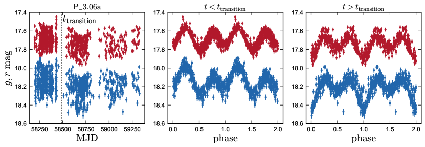
Figure 5: Light curve of P_3.06a, the object with the clearest long-term evolution in the spectroscopic sample. Left panel shows the raw ZTF $g$- and $r$-band light curves. A transition is evident at $\rm MJD\approx 58500$, when the mean brightness decreases by $\approx 0.1$ mag. The middle and right panels show phased light curves from before and after this transition, with phase defined the same way in both panels. An eclipse is evident in the right panel, presumably when the donor is obscured by the disk. The disk was likely brighter before the transition, when no eclipse was evident.

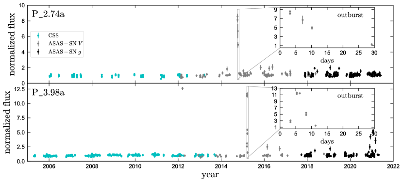
Figure 6: Light curves of two targets with outburst-like events in their observed light curves. Both targets, which are among the coolest (“least evolved”) in our sample, show only one unambiguous dwarf nova-like outburst in 16 years of data. The light curves, from ASAS-SN and CSS, are described in Section 3.5.

3 Spectroscopic sample

To prioritize objects with hot and evolved donors, we obtained follow-up spectra preferentially for candidates that are relatively luminous, with $M_{\rm G}\lesssim 8$ (see lower right panel of Figure 1). For context, ordinary CV donors with $P_{\rm orb}=5$ hours and $P_{\rm orb}=3$ hours have $M_{G}\approx 9.5$ and $M_{G}\approx 12$, respectively. We intentionally selected objects with a range of light curve morphologies. Most of the remaining analysis in this paper is focused on the objects in this spectroscopic sample; properties of the remaining 30 objects can be found in Appendix D.

Table 1 lists basic properties of the sample. Source IDs, Galactic coordinates, apparent magnitudes, and parallaxes are taken from Gaia eDR3 (Gaia Collaboration et al., 2021a). Orbital periods are measured from the ZTF light curves and verified with spectroscopic RVs. We “correct” the reported parallaxes using the position-, color-, and magnitude-dependent parallax zeropoint derived by Lindegren et al. (2021b), and we inflate the reported parallax uncertainties using the empirical inflation formula derived using wide binaries by El-Badry et al. (2021a, their Equation 16). We take reddening values $E(g-r)$ from the Green et al. (2019) 3D dust map; the listed uncertainties account for both reported uncertainties in $E(g-r)$ and for distance uncertainties.

3.1 Kast spectra

We obtained multi-epoch spectra for the 21 targets listed in Table 1 using the Kast double spectrograph (Miller & Stone, 1994) on the 3 m Shane telescope at Lick observatory. Most of the observations were taken during bright time between February and June of 2021; observations for J0140 (P_3.81a) were taken in July and August of 2020 (see El-Badry et al., 2021b). We used the 600/7500 grating on the red side and the 600/4310 grism on the blue side, with the D55 dichroic and a 2 arcsec slit. This results in wavelength coverage of 3300–8400 Å  with typical resolution (FWHM) of 4 Å  on the blue side and 5 Å  on the red side.

Individual exposure times ranged from 5 to 10 minutes, with shorter exposures for brighter targets and objects with shorter orbital periods. The typical single-visit SNR at 6500 Å  ranged from $\approx 10$ for the faintest targets to $\approx 40$ for the brightest. At 4000 Å, the same range was 5 to 20. The SNR of the final coadded spectra is a factor of 3-4 higher. We covered at least half an orbit on almost all targets in order to be able to constrain the radial velocity solution. When possible, all spectra for a given target were obtained in a continuous 2-4 hour period on one night.

To minimize effects of flexure on the wavelength solution, we took a new set of arcs on-sky while tracking each target every $\sim$30 minutes. We reduced the spectra using pypeit (Prochaska et al., 2020), which performs bias and flat field correction, cosmic ray removal, wavelength calibration, flexure correction using sky lines, sky subtraction, extraction of 1d spectra, and heliocentric RV corrections.

We measured RVs in two steps via cross-correlation. We first cross-correlated an ATLAS/SYNTHE model spectrum (Kurucz, 1970, 1979, 1993) with an effective temperature of $T_{\rm eff}=6500\,\rm K$, surface gravity $\log(g/{\rm cm\,s^{-1}})=4.5$, and metallicity [Fe/H]=0 with the observed single-epoch spectra, used the thus-measured RVs to shift all spectra to rest frame, and coadded them. We then fit the resulting coadded spectrum (section 3.2) to obtain atmospheric parameters for a more accurate model. Finally, we use the best-fit model spectrum to repeat the RV measurement and coadding, yielding more accurate RVs. We also re-fit the coadded spectrum to obtain final atmospheric parameters.

The spectra of most objects are dominated by absorption lines from the donor, but more than half show evidence of weak emission, particularly in H$\alpha$, presumably from an accretion disk around the WD. Several objects have clear H$\alpha$ emission lines that rise above the stellar continuum. In others, the H$\alpha$ absorption line is simply weaker than in the best-fit model spectrum, such that emission is visible only in the residuals. In measuring RVs (and in fitting atmospheric parameters), we mask regions of the spectrum with obvious emission lines.

It is worth noting that spectra can change with orbital phase. Indeed, in a few objects with emission lines and eclipses evident in their light curves, we do observe that the emission becomes weaker at phase 0.5, when the disk is obscured by the donor. We do not attempt to correct for such variation in this work, as it primarily affects spectral regions with emission lines, which we mask during fitting.

3.2 Spectral fitting

Table 2: Parameter constraints from fitting spectra (Section 3.2; first 4 columns) and spectral energy distributions (Section 3.4; last 3 columns). The $\log g_{\rm spec+period}$ constraint includes a prior based on the fact that the donors/proto-WDs nearly fill their Roche lobes (Equation 4). The SED fitting takes the spectroscopic effective temperature as a prior; we adopt the spec+SED constraint as the fiducial $T_{\rm eff}$ of the proto-WD in the rest of the paper.

ID	emission?	$T_{\rm eff,\,spec}$	$\log g_{\rm spec+period}$	$\rm[Fe/H]_{\rm spec}$	$T_{\rm eff,\,spec+SED}$	$\Theta_{\rm spec+SED}$	$E(B-V)_{\rm SED+spec}$
		[K]	[dex]	[dex]	[K]	[$\mu$ as]	[mag]
P_2.00a	no	$7646\pm 100$	$5.09\pm 0.10$	$-0.58\pm 0.20$	$7734\pm 73$	$2.44\pm 0.04$	$0.14\pm 0.01$
P_2.74a	yes	$5023\pm 300$	$4.77\pm 0.10$	$0.12\pm 0.40$	$4726\pm 52$	$6.37\pm 0.11$	$0.02\pm 0.01$
P_3.03a	yes	$6096\pm 200$	$4.85\pm 0.10$	$-0.40\pm 0.30$	$5910\pm 77$	$2.44\pm 0.05$	$0.02\pm 0.01$
P_3.06a	yes	$5776\pm 200$	$4.70\pm 0.10$	$-0.02\pm 0.30$	$5862\pm 70$	$2.34\pm 0.05$	$0.04\pm 0.01$
P_3.13a	no	$6331\pm 100$	$4.65\pm 0.10$	$0.25\pm 0.20$	$6662\pm 54$	$4.11\pm 0.06$	$0.08\pm 0.01$
P_3.21a	no	$7051\pm 100$	$4.85\pm 0.10$	$0.25\pm 0.20$	$7022\pm 72$	$3.47\pm 0.06$	$0.41\pm 0.01$
P_3.43a	yes	$5836\pm 200$	$4.84\pm 0.10$	$0.01\pm 0.30$	$6193\pm 83$	$4.12\pm 0.07$	$0.25\pm 0.02$
P_3.48a	yes	$6412\pm 100$	$4.65\pm 0.10$	$-0.26\pm 0.20$	$6444\pm 62$	$2.46\pm 0.04$	$0.01\pm 0.01$
P_3.53a	yes	$5830\pm 200$	$4.70\pm 0.10$	$-0.20\pm 0.30$	$5324\pm 66$	$5.14\pm 0.07$	$0.03\pm 0.02$
P_3.81a	yes	$6665\pm 100$	$4.86\pm 0.10$	$-0.30\pm 0.20$	$6689\pm 72$	$2.12\pm 0.04$	$0.04\pm 0.01$
P_3.88a	yes	$5699\pm 200$	$4.72\pm 0.10$	$-0.00\pm 0.30$	$5875\pm 102$	$3.37\pm 0.08$	$0.09\pm 0.01$
P_3.90a	no	$7396\pm 100$	$4.78\pm 0.10$	$0.18\pm 0.20$	$7442\pm 87$	$3.87\pm 0.06$	$0.06\pm 0.01$
P_3.98a	yes	$5334\pm 300$	$4.58\pm 0.10$	$-0.28\pm 0.40$	$5122\pm 53$	$4.05\pm 0.08$	$0.06\pm 0.01$
P_4.06a	no	$7410\pm 100$	$4.56\pm 0.10$	$-0.48\pm 0.20$	$7587\pm 72$	$3.95\pm 0.06$	$0.21\pm 0.01$
P_4.10a	yes	$5318\pm 200$	$4.60\pm 0.10$	$-0.20\pm 0.30$	$4846\pm 38$	$6.42\pm 0.09$	$0.01\pm 0.01$
P_4.36a	yes	$6139\pm 200$	$4.74\pm 0.10$	$0.15\pm 0.30$	$5998\pm 80$	$3.43\pm 0.07$	$0.10\pm 0.01$
P_4.41a	no	$7315\pm 200$	$4.53\pm 0.10$	$-0.40\pm 0.30$	$7013\pm 105$	$3.94\pm 0.06$	$0.25\pm 0.02$
P_4.47a	no	$6855\pm 200$	$4.71\pm 0.10$	$-0.79\pm 0.30$	$7171\pm 108$	$1.57\pm 0.04$	$0.06\pm 0.01$
P_4.73a	no	$7753\pm 100$	$4.59\pm 0.10$	$-0.32\pm 0.20$	$7619\pm 85$	$4.04\pm 0.06$	$0.31\pm 0.01$
P_5.17a	yes	$6171\pm 200$	$4.42\pm 0.10$	$-0.35\pm 0.30$	$6187\pm 61$	$3.46\pm 0.06$	$0.11\pm 0.01$
P_5.42a	no	$7075\pm 100$	$4.48\pm 0.10$	$-0.52\pm 0.20$	$7326\pm 78$	$6.29\pm 0.09$	$0.34\pm 0.01$

Rest-frame coadded spectra for all targets are shown in Figure 7 and are compared to the best-fit model spectra. Both the observed and model spectra are pseudo-continuum normalized, with the pseudo-continuum defined as a running median of the spectrum calculated in a window of width 150 Å.

We implemented The Payne (Ting et al., 2019; Rix et al., 2016; El-Badry et al., 2018), a framework for interpolating model spectra, to predict the pseudo-continuum normalized spectra of the proto-WD. We use a 2nd order polynomial spectral model with three labels, $\vec{\ell}=\left(T_{{\rm eff}},\log g,\left[{\rm Fe/H}\right]\right)$, which we trained on the BOSZ grid of Kurucz model spectra (Bohlin et al., 2017). In the relevant part of parameter space, the grid spacing is $\Delta T_{\rm eff}=250\,\rm K$, $\Delta\log g=0.5\,\rm dex$, $\Delta[\rm Fe/H]=0.25\,\rm dex$. Once the spectral model is trained, we fit the coadded spectra using a standard maximum likelihood method, where the likelihood function quantifies the difference between the observed and model spectra assuming Gaussian uncertainties.

In the systems with the strongest emission lines (e.g. P_3.98a), emission is obvious in all the Balmer lines and the corresponding absorption lines of the donor are completely filled in. There is also evidence of emission in the Fraunhofer “D3” line at $\approx 5875$ Å  due to neutral helium, and in the Ca H & K lines. In intermediate cases (e.g. P_3.03a), the H$\alpha$ emission rises over the continuum, but the core of the donor’s absorption line is evident as well. In the weakest cases (e.g. P_3.48a) the H$\alpha$ line appears only in absorption but is shallower than predicted by the best-fit spectral model. We show zoomed-in profiles of the H$\alpha$ lines of all targets in Appendix B.

We caution that there is some ambiguity in interpreting the spectra with the weakest emission, because a too-shallow absorption line could also indicate a mismatch between the spectral model and observed spectra. Spectra with higher resolution and SNR will be required to confirm that the tentatively-detected emission in a few objects with $6000<T_{\rm eff}/{\rm K}<7000$ is real. Almost all objects with evidence of a disk in their light curves (eclipses or long-term brightness evolution) also show emission lines. There is one clear exception: the object P_3.13 shows long-term brightness evolution and presumably has a disk, but does not have unambiguous emission lines.

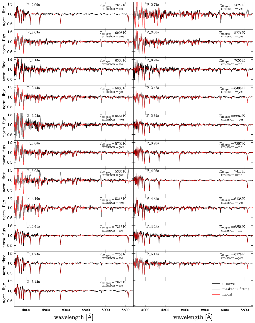
Figure 7: Kast spectra for all targets in the spectroscopic sample. Red lines show the best-fit Kurucz spectral model, with the corresponding effective temperature listed in each panel. Gray regions of the spectra are masked during fitting; these are regions susceptible to contamination from emission lines in targets with evidence of emission. Zoomed-in H$\alpha$ line profiles can be found in Appendix B.

In most cases with evidence for emission, we mask the Balmer lines, He “D3” line, and the Ca H & K lines in fitting. These are the lines most likely to be contaminated by emission, and we find that in most cases other regions of the spectrum are reasonably well-fit by the spectral model. In objects with only weak emission apparent in H$\alpha$, we only mask H$\alpha$.

We use a flat prior on effective temperature and metallicity, $T_{{\rm eff}}/{\rm kK}\sim\mathcal{U}\left(3,10\right)$ and $\left[{\rm Fe/H}\right]\sim\mathcal{U}\left(-2,0.5\right)$. For surface gravity, we use a prior based on the fact that the stars are nearly or complete Roche lobe filling. From Equation 1, we derive

$$\log\left[\frac{g}{{\rm cm\,s^{-2}}}\right]=4.62-\frac{4}{3}\log\left[\frac{P_{{\rm orb}}}{{\rm 4\,hrs}}\right]+\frac{1}{3}\log\left[\frac{M}{0.16\,M_{\odot}}\right]$$ (4)

The expected mass of ELM WDs and evolved CV donors and at these periods is about $0.16\,M_{\odot}$ (e.g. Rappaport et al., 1995; Lin et al., 2011; Chen et al., 2017). We therefore adopt a prior $\log g\sim\mathcal{N}\left(\log g_{0},0.1\right)$, where $\log g_{0}=4.62-\frac{4}{3}\log\left[P_{{\rm orb}}/\left({\rm 4\,hrs}\right)\right]$. The dispersion of 0.1 dex corresponds to a factor of 2 uncertainty in mass (e.g. $0.08<M_{\rm proto\,WD}/M_{\odot}<0.32$) or to a 10% uncertainty in Roche lobe filling factor (e.g. 0.9 rather than 1).

The results of our spectral fitting and inspection for emission lines are listed in the first 4 columns of Table 2. The best-fit model spectra are compared to the data in Figure 7; the fits are reasonably good outside of regions contaminated by emission (gray). As discussed in El-Badry et al. (2021b), the formal uncertainties from our full spectral fitting are often unrealistically small, so we inflate them to plausible values given the SNR and degree of contamination from emission lines. We note that our “final” effective temperatures and surface gravities are respectively derived from the SED (Section 3.4) and the ellipsoidal distortion amplitude (Section 3.7); these are likely more reliable than the values derived from the spectra alone.

One striking feature in Figure 7 is that many objects show excess sodium absorption in the Fraunhofer “D” lines at $\approx$5890 Å. This is true for all objects with $T_{\rm eff}\lesssim 7,000\,\rm K$, the temperature range where the spectra are sensitive to sodium. We have verified that this absorption is not interstellar, but is actually associated with the donor: the line clearly shifts in velocity over the course of the orbit. Such enhancement has also been observed in the spectra of other CVs proposed to have evolved donors (e.g. Thorstensen et al., 2002b). A tempting explanation is that the sodium-enhanced material underwent high-temperature burning in the core of the secondary while it was on the main sequence and subsequent stripping of the star’s envelope exposed this material. Spectra with higher resolution and SNR will test this scenario, which also predicts that other elements, especially C, N, and O, should have anomalous abundances.

3.3 Radial velocities

We fit the RVs of all targets in the spectroscopic sample with a Keplerian model, following the procedure described in El-Badry et al. (2021b). In brief, we fix the orbital period to the value measured from the light curve, and the eccentricity to 0 (since tidal circularization is efficient at such short periods). The measured RVs and best-fit Keplerian orbits are plotted in Figure 8. Our RVs cover more than half of the orbit in nearly all cases (the only exceptions being P_3.53a and P_4.10a), so the RV semi-amplitudes are well-constrained. In several cases (most drastically, P_3.03a), the measured RVs are poorly fit by a Keplerian orbit, in the sense that the difference between the model and data is larger than expected from the reported RV uncertainties. We suspect that this is simply due to instability in the Kast wavelength solution, which is known to drift due to instrument flexure. Our inclusion of a scatter term in the fit accounts for such scatter in a controlled way, effectively inflating the observational uncertainties until the reduced $\chi^{2}$ is of order unity.

The orbital semi-amplitude and period constrain the mass-function, $f_{m}$, which represents the minimum possible mass of the object the proto-WD is orbiting. It is given by

$$f_{m} =M_{{\rm WD}}\left(\frac{M_{{\rm WD}}}{M_{{\rm WD}}+M_{{\rm proto\,WD}}}\right)^{2}\sin^{3}i=\frac{P_{{\rm orb}}K_{{\rm proto\,WD}}^{3}}{2\pi G}$$ (5)

$$=0.47\,M_{\odot}\times\left(\frac{P_{{\rm orb}}}{4\,{\rm hr}}\right)\left(\frac{K_{{\rm proto\,WD}}}{300\,{\rm km\,s^{-1}}}\right)^{3},$$ (6)

where $M_{\rm WD}$ represents the mass of the unseen companion, here presumed to be a WD. $f_{m}$ is the mass that the companion would have if the proto-WD were a massless test particle and the inclination were 90 degrees, so the actual mass of the companion can only be higher.

Table 3: Orbital solutions from fitting RVs. $K_{\rm proto\,WD}$ is the RV semi-amplitude of the secondary, $\gamma$ is the center-of-mass RV, and $f_{m}$ is the mass function of the unseen companion (Equation 5). The period and conjunction time are fixed to the light curve-derived values, and the eccentricity is set to 0. The RV zeropoint of the Kast spectra is uncertain at the $30\,\rm km\,s^{-1}$ level; this should be treated as an additional systematic error in interpreting $\gamma$ (but not $K_{\rm proto\,WD}$) values.

ID	$K_{\rm proto\,WD}$	$\gamma$	$f_{m}$
	[$\rm km\,s^{-1}$]	[$\rm km\,s^{-1}$]	[$M_{\odot}$]
P_2.00a	$368\pm 9$	$-48\pm 8$	$0.43\pm 0.03$
P_2.74a	$320\pm 12$	$-76\pm 10$	$0.39\pm 0.05$
P_3.03a	$320\pm 12$	$19\pm 9$	$0.44\pm 0.05$
P_3.06a	$269\pm 8$	$-46\pm 9$	$0.26\pm 0.02$
P_3.13a	$324\pm 15$	$-49\pm 12$	$0.48\pm 0.07$
P_3.21a	$333\pm 11$	$22\pm 7$	$0.50\pm 0.05$
P_3.43a	$290\pm 7$	$53\pm 6$	$0.36\pm 0.03$
P_3.48a	$274\pm 5$	$-14\pm 4$	$0.31\pm 0.02$
P_3.53a	$314\pm 30$	$-12\pm 22$	$0.49\pm 0.14$
P_3.81a	$324\pm 6$	$-55\pm 4$	$0.56\pm 0.03$
P_3.88a	$282\pm 7$	$-58\pm 5$	$0.38\pm 0.03$
P_3.90a	$331\pm 5$	$16\pm 3$	$0.61\pm 0.03$
P_3.98a	$273\pm 10$	$-37\pm 8$	$0.35\pm 0.04$
P_4.06a	$283\pm 7$	$-9\pm 6$	$0.40\pm 0.03$
P_4.10a	$288\pm 22$	$-60\pm 18$	$0.43\pm 0.10$
P_4.36a	$295\pm 7$	$-9\pm 5$	$0.48\pm 0.03$
P_4.41a	$274\pm 4$	$-107\pm 3$	$0.39\pm 0.02$
P_4.47a	$286\pm 15$	$-78\pm 9$	$0.46\pm 0.08$
P_4.73a	$249\pm 5$	$-115\pm 5$	$0.32\pm 0.02$
P_5.17a	$200\pm 9$	$3\pm 7$	$0.18\pm 0.02$
P_5.42a	$250\pm 6$	$-122\pm 3$	$0.37\pm 0.03$

Table 3 lists the measured RV semi-amplitudes, center-of-mass velocities, and mass functions for all objects in the spectroscopic sample. The mass functions range from $0.18$ to $0.61M_{\odot}$, all consistent with WD companions. We constrain the masses of the companions in Section 3.7.

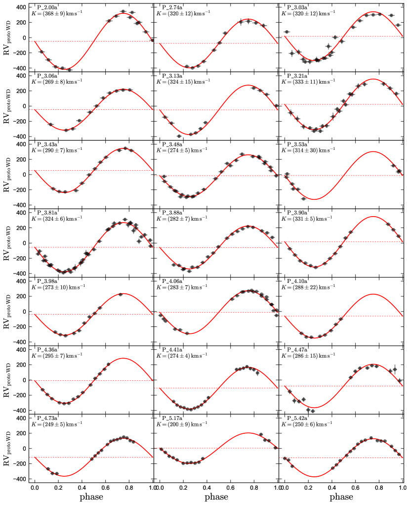
Figure 8: Kast RVs for all targets. Points with errorbars show measured RVs; red line shows the best-fit orbital solution. Dashed lines show the corresponding systemic velocity. The measured RVs cover at least half an orbit and allow for a well-constrained orbital solution for almost all systems.

3.4 Spectral energy distributions and angular diameters

We retrieved available UV-to-IR photometry for targets in the spectroscopic sample and used it to constrain the donors’ effective temperatures, angular diameters, and color excesses. We use photometry for all targets from Pan-STARRS1 (Kaiser et al., 2002), 2MASS (Skrutskie et al., 2006), and WISE (Wright et al., 2010). The resulting spectral energy distributions (SEDs) are shown in Figure 9, with the reported apparent magnitudes converted to flux densities using the appropriate zeropoints for each survey. We also show photometry from GALEX (Martin et al., 2005) where available. We do not use it in fitting, because we expect the WD companion and/or accretion disk to often contribute significantly in the UV.

In most cases, the SED can independently constrain the effective temperature and angular diameter: the wavelength at which the SED begins to turn over constrains $T_{\rm eff}$, and the normalization of the SED constrains $\Theta$, the angular diameter. Particularly when IR photometry is available, the resulting constraints on the angular diameter and temperature are quite precise (e.g. Blackwell & Shallis, 1977). The effective temperatures of objects in our sample, $4,500\lesssim T_{\rm eff}/{\rm K}\lesssim 8,000$, lead to SEDs that peak between 3,700 and 6,500 Å, so the flattening of the SED near the peak is always probed by the Pan-STARRS grizy photometry.

We predict bandpass-averaged mean magnitudes of the proto-WD using empirically-calibrated theoretical models from the BaSeL library (v2.2; Lejeune et al., 1997, 1998). We fix $\log g=4.75$ and $Z=0.014$ in calculating model magnitudes, since varying $\log g$ and metallicity at fixed angular diameter has only minor effects on the SED. We assume a Cardelli et al. (1989) extinction law with total-to-selective extinction ratio $R_{V}=3.1$. We use pystellibs to interpolate between model spectra, and pyphot to calculate synthetic photometry. These calculations treat the proto-WD as spherical, neglecting the effects of tidal distortion and gravity darkening.

Some care must be taken in interpreting the observed magnitudes, since the expected brightness of these sources depends on when they are observed. The magnitudes reported by Pan-STARRS and WISE represent the mean of many exposures from different visits (typically 12 for Pan-STARRS and 20-80 for WISE) and are therefore expected to reflect the phase-averaged mean magnitude reasonably accurately. We add 0.03 mag in quadrature to the reported photometric uncertainties to account for the random sampling of observations in phase as well as photometric calibration uncertainties.

Unlike the Pan-STARRS and WISE data, the 2MASS magnitudes were in most cases calculated from only one visit and thus represent the source brightness at a random phase. Because the 2MASS exposures were obtained $\approx 20$ years before the ZTF data, it is not always possible to accurately calculate the phase at which they were obtained. Rather than attempting to correct them for phase variability, we therefore simply inflate the 2MASS uncertainties by adding 0.1 mag in quadrature to the reported photometric uncertainties. This has little effect on our constraints, because both the 2MASS and WISE data are in the Rayleigh-Jeans tail of the SED for all sources, and WISE data are available for all objects.

We do not attempt to model an accretion disk or companion WD in our fits of the SED. Because emission lines are weak or absent for most sources and the Kurucz model spectra do not significantly over-predict the depth of most absorption lines, we expect that the fraction of the optical flux contributed by the disk is generally small. The companion WD’s contributions are also expected to be small (few percent) for plausible masses and temperatures. Still, in systems with emission, it is generally not possible to exclude disks that contribute to the optical flux at the 10-20% level. We discuss the effects of unrecognized flux from a disk in Section 3.4.1.

We adopt priors on the color excess for each target based on the 3D dust map from Green et al. (2019); these values are listed in Table 1. We convert the reported $g-r$ color excess a to $B-V$ color excess using $E(B-V)=0.98E(g-r)$, as is appropriate for a Cardelli et al. (1989) extinction law with $R_{V}=3.1$. The effective temperature constraints obtained from fitting normalized spectra (Table 2) are also adopted as priors. For the angular diameter, we use a flat prior, $\Theta_{{\rm proto\,WD}}\,\left[{\rm\mu\,as}\right]\sim\mathcal{U}\left(0,10\right)$. Here $\Theta_{{\rm proto\,WD}}=2R_{{\rm proto\,WD}}/d$ is the angular diameter of the proto-WD donor, where $R_{\rm proto\,WD}$ is its radius and $d$ is the distance to the system. We fit the SEDs using emcee (Foreman-Mackey et al., 2013) to sample from the posterior, monitoring chains for convergence. The resulting constraints on the effective temperatures and angular diameters of the proto WDs are listed in Table 2.

The best-fit model SED for each system is compared to the observed data in Figure 9. The data used in the fit is shown in gray; UV photometry from GALEX is shown in cyan where available but is not considered in fitting. Some of the sources without GALEX photometry are outside the mission’s survey footprint; others are within the footprint but were not detected in the UV. Several systems have NUV but not FUV detections; most of these are in fields that GALEX observed after the failure of the FUV detector. The best-fit effective temperatures, angular diameters, and color excesses are listed in each panel; we also note whether emission is evident in the spectrum. Constraints are tabulated in Table 2.

The SED fits are generally good. The inferred effective temperatures are in most cases consistent with those inferred from spectral fitting (the median absolute difference is 190 K), and the best-fit $E(B-V)$ values are similar to those predicted by the Green et al. (2019) dust map. None of the sources show evidence of IR excess. Most of the sources detected by GALEX have UV excess, meaning the observed UV fluxes are larger than predicted by the model for the proto-WD alone. This excess can originate either from the WD companion (irrespective of whether it is accreting), or from the inner regions of the accretion disk, if one exists. Most, but not all, of the systems with UV excess also show emission in their spectra. This is expected, since accretion both gives rise to emission lines and keeps the WD hot (e.g. Townsley & Gänsicke, 2009). On the other hand, a hot WD companion does not guarantee that there is ongoing accretion: for plausible companion WD masses and luminosities in our sample, it would take the WD of order 100 Myr to cool enough that it would no longer be detected in the UV.

3.4.1 Effects of possible unaccounted flux from the disk or companion WD

Besides emitting in the UV, the WD companion and/or accretion disk could also contribute in the optical, complicating the interpretation of our inferred angular diameters. Given the low accretion rates expected for evolved CVs (see El-Badry et al., 2021b) and the large masses we infer dynamically (Section 3.7), we generally expect the companion WDs to contribute negligibly in the optical. The situation is more complicated for disks, which, depending on accretion rate and stability, can have a wide range of temperatures and SED shapes (e.g. Warner, 2003). For normal CVs, it would not be a reasonable approximation to neglect the disk, which typically dominates in the optical. This is not the case for objects in our sample, whose spectra are clearly dominated by the donors and whose optical-to-IR SEDs are reasonably well-fit by pure stellar models.

Nevertheless, the angular diameters we derive are, strictly speaking, upper limits: if the disk contributes additional flux to the SED that is not accounted for, the donor angular diameter will typically be overestimated. If the donor effective temperature is well-constrained and an unaccounted-for disk contributes $f$ times the flux of the donor, then the donor angular diameter will be overestimated by a factor of $\sqrt{1+f}$, and the mass by a factor $\left(1+f\right)^{3/2}$ (e.g. Equation 1). Neglecting a 10% (20%) flux contribution from a disk would thus lead to a radius over-estimate of 5% (10%) and a mass over-estimate of 15% (31%).

There are three objects in the sample for which there is fairly strong evidence that the disk’s emission is not negligible in the optical: P_3.06a, P_3.98a, and P_4.10a. In the first case, the light curve shows a strong secular brightness change due to a change in the disk structure (Figure 5). In the 2nd, there are relatively strong emission lines in the spectrum (Figure 7), and the scatter is significantly larger in the $g$ band than in the $r$ band. In the third, there is a significant asymmetry in the light curve, most likely due to a disk (Figure 4). For these three objects, we explicitly interpret the inferred proto-WD radii and masses (Section 3.7) as upper limits.

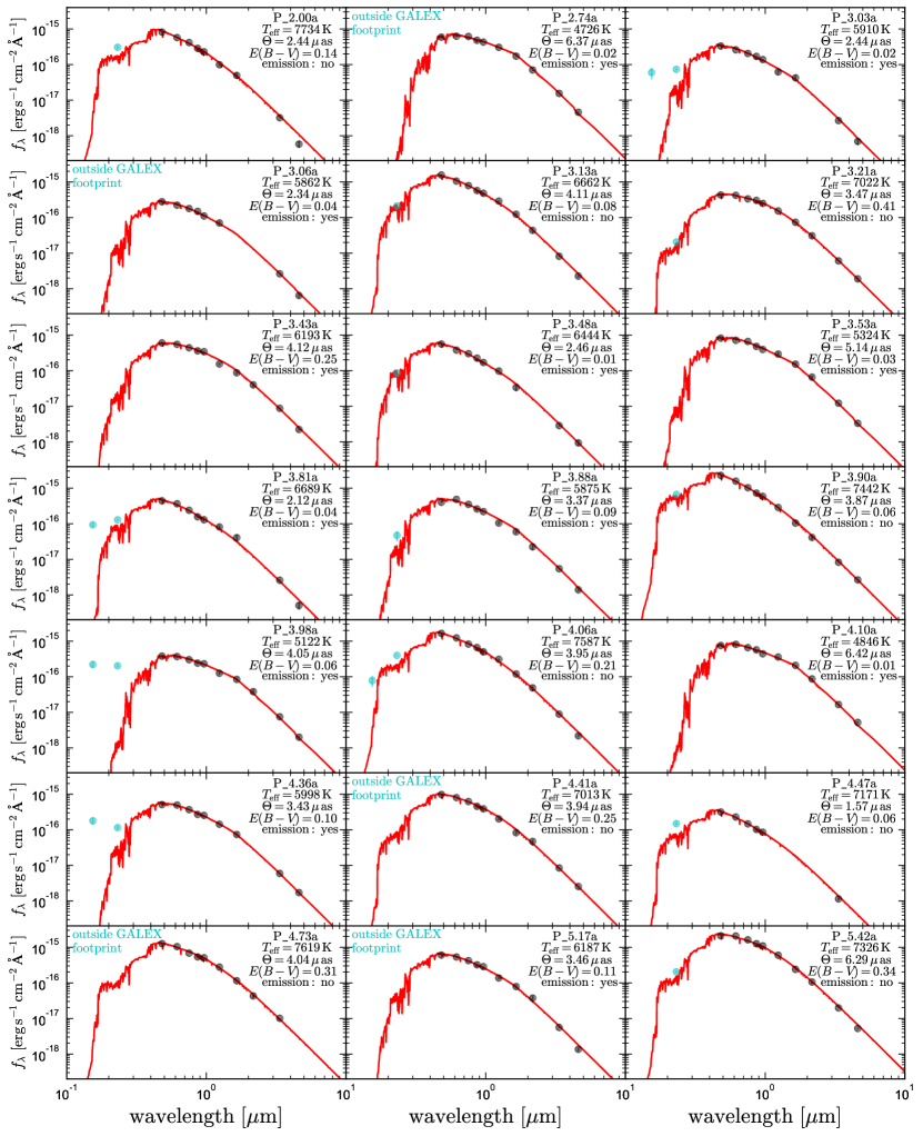
Figure 9: Spectral energy distributions of all targets. Gray points show observed optical-to-IR broadband fluxes from Pan-STARRS, 2MASS, and WISE. Red lines show the best-fit stellar models for the proto-WD, with the effective temperature, angular diameter, and reddening for each object listed. Cyan points show UV fluxes from GALEX. These are not included in the fits, because the WD companion and/or accretion disk are often expected to contribute significantly there.

3.5 Orbital ephemerides

We constrain the orbital ephemeris of each target in the spectroscopic sample by fitting available light curve data from several surveys with a Fourier model, following the same procedure described for the ZTF data in Section 2.4. The highest-quality light curves are from ZTF. However, these only cover $\sim$3 years. A significantly tighter constraint on the orbital period can be obtained by including light curve data with a longer time baseline. To this end, we retrieved light curves for all targets, where available, from the Catalina Sky Survey (CSS; Drake et al., 2009) and the All-Sky Automated Survey for Supernovae (ASAS-SN; Kochanek et al., 2017), and we included normalized light curves from all surveys in a joint fit. Where CSS data are available, the full light curves span 15-16 years (25 to 70 thousand orbits). We remove outbursts and other outliers in fitting. CSS data are deep enough for all our targets within its footprint to be detected. ASAS-SN data only rarely include defections fainter than $V\approx 17$, so we only include ASAS-SN data in the fit for targets with $G<16.75$.

The resulting ephemerides are listed in Table 4. The conjunction times represent the time when the proto-WD would be eclipsed (if viewed edge-on) by its companion. The conjunction times we report are chosen to lie roughly at the median observation time of the data included in fitting, in order to reduce covariance between $T_{0}$ and $P_{\rm orb}$.

Table 4: Orbital ephemerides from light curve fitting. The conjunction time, $T_{0}$, is the time corresponding to phase 0, when the WD passes in front of the proto-WD.

ID	$P_{\rm orb}$	$T_{0}$
	[days]	[MHJD UTC]
P_2.00a	0.08331301(2)	56410.887(1)
P_2.74a	0.11414278(4)	56489.326(2)
P_3.03a	0.12642666(6)	56473.433(1)
P_3.06a	0.1274832(2)	58693.285(1)
P_3.13a	0.13056512(8)	56431.158(2)
P_3.21a	0.13375228(7)	56454.278(2)
P_3.43a	0.1429875(2)	58718.598(1)
P_3.48a	0.14479504(6)	56350.953(1)
P_3.53a	0.1468830(3)	58717.743(1)
P_3.81a	0.15863390(7)	56437.637(1)
P_3.88a	0.1615714(3)	58717.825(1)
P_3.90a	0.1624549(1)	58339.258(1)
P_3.98a	0.16582294(9)	56355.722(2)
P_4.06a	0.16898413(4)	56411.414(1)
P_4.10a	0.1708102(4)	58718.202(2)
P_4.36a	0.1817430(2)	58699.314(1)
P_4.41a	0.1838691(2)	58717.946(2)
P_4.47a	0.18604299(9)	56351.560(2)
P_4.73a	0.1969063(2)	58724.817(1)
P_5.17a	0.2153735(2)	56346.919(2)
P_5.42a	0.2258108(1)	56548.226(2)

3.6 Light curve models

We next explore constraints on the orbital inclination and the Roche lobe filling factor of the proto-WD, $f_{\rm proto\,WD}=R_{\rm proto\,WD}/R_{\rm Roche\,lobe}$, that can be obtained from the light curves. We first consider the case of light curves that only show evidence of ellipsoidal variability (no eclipses) and are not known to be mass-transferring.

The amplitude of ellipsoidal variability in a tidally distorted star depends on the inclination, Roche lobe filling factor, mass ratio, and effective temperature (through the gravity and limb-darkening laws). For our sample, the effective temperature is well-constrained from spectra and SEDs. The mass ratio is not known, but given the large mass functions and our prior that the donors are proto-WDs, it is reasonable to assume $M_{\rm WD}/M_{\rm proto\,WD}\gg 1$. In this limit, the dependence on mass ratio is weak.

This is illustrated in the left panel of Figure 10, which shows the predicted $g-$band variability amplitude for a proto-WD with temperature and mass ratio characteristic of our sample and a range of inclinations and filling factors. We calculate light curves with Phoebe (Prša & Zwitter, 2005; Prša et al., 2016; Horvat et al., 2018) for two different mass ratios. For a typical proto-WD mass of $\approx 0.15M_{\odot}$, these correspond to WD companion masses of $0.6$ and $0.9M_{\odot}$. In the limit of $M_{\rm WD}/M_{\rm proto\,WD}\gg 1$, the ellipsoidal variability amplitude scales roughly as $\propto\sin^{2}i\times f_{\rm proto\,WD}^{3}$ (e.g. Morris & Naftilan, 1993; Gomel et al., 2021). All the objects in our sample have peak-to-peak variability amplitudes greater than 15%; Figure 10 shows that this implies a Roche lobe filling factor greater than $\approx 0.8$ and an inclination greater than $\approx 45$ degrees.

The right panel of Figure 10 shows the locus in the inclination–filling factor plane that is implied by the measured variability amplitude for non-eclipsing objects in the spectroscopic sample. We first calculated these assuming $M_{\rm WD}/M_{\rm proto\,WD}=4.66$, with $M_{\rm proto\,WD}=0.15\,M_{\odot}$ and $M_{\rm WD}=0.7\,M_{\odot}$. After fitting for the masses of both components (Section 3.7), we updated the mass ratios assumed in calculating the tracks, proceeding iteratively until the solution converged. As one might expect, the objects with the largest variability amplitudes are confined to a small range of plausible inclinations and filling factors, while those with lower amplitudes are consistent with a wider range.

In fitting for the masses of the proto-WDs, we require the systems that do not have emission lines (and thus may not be undergoing mass transfer) to fall along the tracks shown in the right panel of Figure 10. For systems with emission lines, we assume that there is ongoing mass transfer and thus fix $f_{\rm proto\,WD}=1$. We still leave the inclination free in these systems, since a disk may change the variability amplitude from what is predicted due to ellipsoidal variation alone.

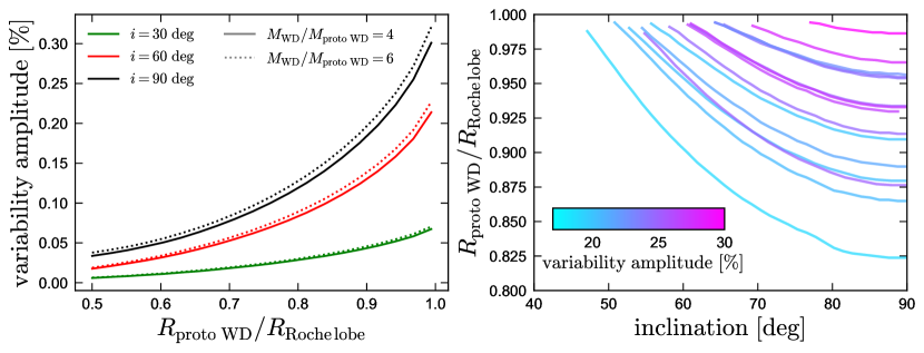
Figure 10: Left: predicted peak-to-peak ellipsoidal variability amplitude for a 7000 K proto-WD viewed at three different inclinations. We compare predictions for two different mass ratios plausible for our sample, which are very similar. Only binaries with $R_{\rm proto\,WD}/R_{\rm Roche\,lobe}\gtrsim 0.8$ and inclinations $i\gtrsim 45\,\rm deg$ reach the variability amplitudes greater than 15% required to enter our sample. Right: Roche lobe filling factor of the proto white dwarf as a function of inclination, as implied by the observed ellipsoidal variability amplitude. The systems with the highest variability amplitude (magenta) must be nearly Roche filling and have high inclination. Systems with lower variability amplitude are consistent with a wider range of inclinations and filling factors. Variability amplitude also depends on effective temperature (through temperature-dependent gravity-darkening), leading to some non-monotonicity in this plane. We only consider systems here in which the variability can be well-described by ellipsoidal variation, excluding systems with eclipses.

3.7 Combined fits

We carry out a simultaneous fit for the masses of both components, the Roche lobe filling factor of the proto WD, distance, and inclination. The “inputs” to the fit are the angular diameter from the SED fit, the RV semi-amplitude from the spectroscopic orbit fit, and the corrected Gaia parallax (Table 1). Following the procedure described in El-Badry et al. (2021b), we use a Markov chain Monte Carlo method to explore what range of parameter space is consistent with all observables, and the covariances between parameters.

3.7.1 Sources with emission lines

For objects with emission lines, which are presumed to be mass transferring and thus must fill their Roche lobes, we fix $R_{\rm proto\,WD}/R_{\rm Roche\,lobe}=1$. The likelihood function is then

$$\ln L_{\rm emission}= -\frac{1}{2}\frac{\left(K_{{\rm model}}-K_{{\rm obs}}\right)^{2}}{\sigma_{K,{\rm obs}}^{2}}-\frac{1}{2}\frac{\left(\Theta_{{\rm model}}-\Theta_{{\rm obs}}\right)^{2}}{\sigma_{\Theta,\,{\rm obs}}^{2}}$$

$$-\frac{1}{2}\frac{\left(\varpi_{{\rm model}}-\varpi_{{\rm obs}}\right)^{2}}{\sigma_{\varpi,\,{\rm obs}}^{2}}.$$

The three terms compare the proto-WD’s predicted RV semi-amplitude and angular diameter, and the system parallax, to the observed constraints, which are respectively taken from Tables 3, 2, and 1. The predicted RV semi-amplitude of the proto-WD is

$$K_{{\rm model}} =\frac{\left[2\pi G\left(M_{{\rm proto\,WD}}+M_{{\rm WD}}\right)/P_{\rm orb}\right]^{1/3}}{\left(1+M_{{\rm proto\,WD}}/M_{{\rm WD}}\right)}\sin i,$$ (7)

the model parallax is $\varpi_{\rm model}=1/d$, and the angular diameter is $\Theta_{{\rm model}}=2R_{\rm proto\,WD}/d$.

We use flat priors on the masses of both components. We take the distance prior from Bailer-Jones et al. (2020):

$$P\left(d\right)=\begin{cases}\frac{1}{\Gamma\left(\frac{\beta+1}{\alpha}\right)}\frac{\alpha}{L^{\beta+1}}d^{\beta}e^{-\left(d/L\right)^{\alpha}},&{\rm if}\,d\geq 0\\ 0,&{\rm otherwise}\end{cases}$$ (8)

Here $L$, $\alpha$, and $\beta$ are free parameters that depend on sky position and are provided by Bailer-Jones et al. (2020). They were calculated by fitting the distance distribution of sources in a mock Gaia eDR3 catalog (Rybizki et al., 2020); we query the appropriate values of $L$, $\alpha$, and $\beta$ for the sky position of each source. None of our results are sensitive to this prior, since they all have high signal-to-noise parallaxes. The median parallax_over_error for the spectroscopic sample is 22.

For the inclination, we use a $\sin i$ prior (as appropriate for random orbit orientations) between $i_{\rm min}$ and 90 degrees. The minimum allowed inclination $i_{\rm min}$ is listed together with our results in Table 5. For objects without eclipses, it is the minimum allowed value given the observed ellipsoidal amplitude; i.e., the minimum inclination for each source in the right panel of Figure 10. We note that dilution of variability from a (non-eclipsing) disk would reduce the variability amplitude, only leading to a tighter constraint on the inclination than we impose. For objects whose light curves show evidence of eclipses, we take $i_{\rm min}=70$ deg.

3.7.2 Sources without emission lines

Sources without emission lines are presumed to be detached, so we leave the Roche lobe filling factors free in fitting and require the binary to fall along the appropriate locus in inclination/filling factor space. We note (see Appendix C) that at least one object without emission lines (P_3.13a) may still be mass-transferring. The likelihood function is:

$$\ln L_{\rm no\,emission}= -\frac{1}{2}\frac{\left[i_{{\rm model}}-i_{{\rm light\,curve\,|}f_{\rm proto\,WD}}\right]^{2}}{\sigma_{i}^{2}}$$

$$-\frac{1}{2}\frac{\left(K_{{\rm model}}-K_{{\rm obs}}\right)^{2}}{\sigma_{K,{\rm obs}}^{2}}-\frac{1}{2}\frac{\left(\Theta_{{\rm model}}-\Theta_{{\rm obs}}\right)^{2}}{\sigma_{\Theta,\,{\rm obs}}^{2}}$$

$$-\frac{1}{2}\frac{\left(\varpi_{{\rm model}}-\varpi_{{\rm obs}}\right)^{2}}{\sigma_{\varpi,\,{\rm obs}}^{2}}$$

Here $i_{\rm model}$ is the inclination (a free parameter), and $i_{{\rm light\,curve\,|}f_{\rm proto\,WD}}$ represents the inclination that, for a particular Roche lobe filling factor, would produce the observed ellipsoidal amplitude (right panel of Figure 10). We adopt $\sigma_{i}=2\,\rm deg$, allowing for a small amount of scatter around this constraint. The other terms in the likelihood are the same as in the case with emission lines. We also use the same priors, but add a prior on the Roche lobe filling factor (see Appendix A) that is motivated by binary evolution calculations and favors filling factors near unity.

4 Results

The constraints from the combined fits for all 21 objects with spectroscopic follow-up are listed in Table 5. We translate the constraints on the Roche lobe filling factor to constraints on the physical radius of the proto WD using the fitting function from Eggleton (1983):

$$R_{{\rm Roche\,lobe}}\approx\frac{0.49q^{2/3}}{0.6q^{2/3}+\ln\left(1+q^{1/3}\right)}\times a,$$ (9)

where $q=M_{\rm proto\,WD}/M_{\rm WD}$ and $a$ is the semi-major axis, which from Kepler’s 3rd law is

$$a=\left(\frac{P_{\rm orb}^{2}G\left(M_{{\rm proto\,WD}}+M_{{\rm WD}}\right)}{4\pi^{2}}\right)^{1/3}.$$ (10)

We calculate $R_{{\rm proto\,WD}}=f_{\rm proto\,WD}\times R_{{\rm Roche\,lobe}}$ directly from the MCMC samples, thus propagating the uncertainties and parameter covariances. We similarly calculate the surface gravity, $\log g_{{\rm proto\,WD}}=\log\left[GM_{{\rm proto\,WD}}/R_{{\rm proto\,WD}}^{2}\right]$, to facilitate comparison of our sample to objects with spectroscopically measured $\log g$, the luminosity, $L_{\rm proto\,WD}=\left(R_{{\rm proto\,WD}}/R_{\odot}\right)^{2}\left(T_{{\rm eff,\,proto\,WD}}/5780\,{\rm K}\right)^{4}L_{\odot}$, and the gravitational wave inspiral time (Peters, 1964),

$$\tau_{{\rm inspiral}}=\frac{5c^{5}}{256G^{5/3}}\frac{\left(M_{{\rm proto\,WD}}+M_{{\rm WD}}\right)^{1/3}}{M_{{\rm proto\,WD}}M_{{\rm WD}}}\left(\frac{P_{{\rm orb}}}{2\pi}\right)^{8/3}$$

An example of the typical covariances between parameters can be found in El-Badry et al. (2021b, their Figure 9). In all cases, distance and the mass and radius of the proto-WD are covariant, with a positive correlation, and $M_{\rm WD}$ is correlated with $M_{\rm proto\,WD}$ and anti-correlated with inclination. For most objects in our sample, the parallax uncertainty is the dominant source of uncertainty in the masses and radii of the proto-WDs. The mass of a proto-WD that fills or nearly fills its Roche lobe can be calculated via Equation 1 to be

$$M_{{\rm proto\,WD}}=0.16\,M_{\odot}\left(\frac{\Theta_{{\rm proto\,WD}}}{3\,\mu{\rm as}}\right)^{3}\left(\frac{P_{{\rm orb}}}{4\,{\rm hr}}\right)^{-2}\left(\frac{\varpi}{{\rm mas}}\right)^{-3}.$$ (11)

This means that when parallax errors dominate and are small enough to justify a linear error analysis, the expected fractional mass uncertainty is

$$\frac{\sigma_{M_{{\rm proto\,WD}}}}{M_{{\rm proto\,WD}}}\approx 3\frac{\sigma_{\varpi}}{\varpi},$$ (12)

so that a 20% (5%) parallax uncertainty translates to a 60% (15%) mass uncertainty.

Table 5: Combined fitting results. $M_{\rm proto\,WD}$, $f_{\rm proto\,WD}=R_{\rm proto\,WD}/R_{\rm Roche\,lobe}$, $M_{\rm WD}$, $d$, and $i$ are fitting parameters; $R_{\rm proto\,WD}$, $\log g_{\rm proto\,WD}$, and $\tau_{\rm inspiral}$ are derived. $i_{\rm min}$ and $f_{\rm proto\,WD,\,min}$ are calculated from the observed ellipsoidal variability amplitude and set the lower limits of $i$ and $f_{\rm proto\,WD}$ in fitting.

ID	$M_{\rm proto\,WD}$	$R_{\rm proto\,WD}$	$\log g_{{\rm proto\,WD}}$	$M_{\rm WD}$	$d$	$i$	$f_{\rm proto\,WD}$	$\tau_{\rm inspiral}$	$i_{\rm min}$	$f_{\rm proto\,WD,\,min}$
	[$M_{\odot}$]	[$R_{\odot}$]	[$\rm cm\,s^{-2}$]	[$M_{\odot}$]	[kpc]	deg		[Gyr]	[deg]
P_2.00a	$0.13_{-0.02}^{+0.03}$	$0.17_{-0.01}^{+0.01}$	$5.06_{-0.07}^{+0.10}$	$0.98_{-0.21}^{+0.18}$	$0.66_{-0.02}^{+0.03}$	$55.49_{-5.33}^{+14.14}$	$0.94_{-0.07}^{+0.05}$	$0.53_{-0.08}^{+0.09}$	46	0.82
P_2.74a	$0.13_{-0.01}^{+0.01}$	$0.23_{-0.01}^{+0.01}$	$4.84_{-0.01}^{+0.01}$	$0.62_{-0.06}^{+0.06}$	$0.34_{-0.00}^{+0.00}$	$79.76_{-6.75}^{+7.00}$	$1.00_{-0.00}^{+0.00}$	$1.59_{-0.16}^{+0.18}$	70	1.00
P_3.03a	$0.17_{-0.05}^{+0.07}$	$0.27_{-0.03}^{+0.03}$	$4.81_{-0.05}^{+0.05}$	$0.77_{-0.11}^{+0.14}$	$1.02_{-0.10}^{+0.13}$	$73.10_{-9.92}^{+11.29}$	$1.00_{-0.00}^{+0.00}$	$1.45_{-0.49}^{+0.68}$	59	1.00
P_3.06a	$0.18_{-0.04}^{+0.05}$	$0.27_{-0.02}^{+0.03}$	$4.81_{-0.03}^{+0.04}$	$0.51_{-0.06}^{+0.06}$	$1.09_{-0.09}^{+0.10}$	$79.49_{-6.61}^{+7.09}$	$1.00_{-0.00}^{+0.00}$	$1.91_{-0.53}^{+0.67}$	70	1.00
P_3.13a	$0.18_{-0.02}^{+0.02}$	$0.28_{-0.01}^{+0.01}$	$4.81_{-0.02}^{+0.02}$	$0.74_{-0.08}^{+0.09}$	$0.63_{-0.02}^{+0.03}$	$83.66_{-2.75}^{+4.65}$	$1.00_{-0.01}^{+0.00}$	$1.49_{-0.22}^{+0.26}$	76	0.98
P_3.21a	$0.24_{-0.05}^{+0.06}$	$0.31_{-0.02}^{+0.02}$	$4.84_{-0.03}^{+0.04}$	$0.95_{-0.09}^{+0.10}$	$0.83_{-0.06}^{+0.06}$	$71.56_{-3.18}^{+7.29}$	$0.99_{-0.01}^{+0.01}$	$1.02_{-0.24}^{+0.30}$	64	0.95
P_3.43a	$0.12_{-0.02}^{+0.02}$	$0.26_{-0.01}^{+0.01}$	$4.69_{-0.02}^{+0.02}$	$0.57_{-0.04}^{+0.05}$	$0.58_{-0.03}^{+0.03}$	$79.21_{-6.44}^{+7.31}$	$1.00_{-0.00}^{+0.00}$	$3.43_{-0.56}^{+0.64}$	70	1.00
P_3.48a	$0.11_{-0.03}^{+0.04}$	$0.26_{-0.02}^{+0.02}$	$4.67_{-0.04}^{+0.04}$	$0.53_{-0.06}^{+0.09}$	$0.97_{-0.08}^{+0.09}$	$73.90_{-10.57}^{+11.05}$	$1.00_{-0.00}^{+0.00}$	$3.89_{-1.06}^{+1.42}$	59	1.00
P_3.53a	$0.20_{-0.02}^{+0.02}$	$0.32_{-0.01}^{+0.01}$	$4.75_{-0.01}^{+0.01}$	$0.83_{-0.16}^{+0.19}$	$0.57_{-0.02}^{+0.02}$	$79.66_{-6.67}^{+6.96}$	$1.00_{-0.00}^{+0.00}$	$1.69_{-0.29}^{+0.37}$	70	1.00
P_3.81a	$0.24_{-0.09}^{+0.16}$	$0.35_{-0.05}^{+0.07}$	$4.73_{-0.07}^{+0.07}$	$0.96_{-0.13}^{+0.18}$	$1.54_{-0.22}^{+0.29}$	$78.34_{-7.71}^{+7.76}$	$1.00_{-0.00}^{+0.00}$	$1.59_{-0.71}^{+1.11}$	67	1.00
P_3.88a	$0.12_{-0.02}^{+0.02}$	$0.28_{-0.01}^{+0.02}$	$4.62_{-0.02}^{+0.02}$	$0.59_{-0.04}^{+0.05}$	$0.78_{-0.03}^{+0.04}$	$79.64_{-6.60}^{+6.96}$	$1.00_{-0.00}^{+0.00}$	$4.56_{-0.78}^{+0.90}$	70	1.00
P_3.90a	$0.22_{-0.03}^{+0.03}$	$0.33_{-0.01}^{+0.01}$	$4.73_{-0.04}^{+0.05}$	$1.17_{-0.13}^{+0.10}$	$0.80_{-0.02}^{+0.03}$	$64.85_{-4.42}^{+10.19}$	$0.97_{-0.03}^{+0.03}$	$1.61_{-0.19}^{+0.21}$	57	0.96
P_3.98a	$0.32_{-0.06}^{+0.08}$	$0.40_{-0.03}^{+0.03}$	$4.74_{-0.03}^{+0.03}$	$0.84_{-0.12}^{+0.19}$	$0.91_{-0.06}^{+0.07}$	$70.36_{-12.32}^{+13.16}$	$1.00_{-0.00}^{+0.00}$	$1.52_{-0.39}^{+0.50}$	53	1.00
P_4.06a	$0.12_{-0.02}^{+0.02}$	$0.28_{-0.01}^{+0.01}$	$4.63_{-0.05}^{+0.08}$	$0.81_{-0.13}^{+0.12}$	$0.65_{-0.02}^{+0.02}$	$59.48_{-5.30}^{+12.19}$	$0.95_{-0.05}^{+0.04}$	$4.10_{-0.45}^{+0.51}$	54	0.89
P_4.10a	$0.25_{-0.02}^{+0.03}$	$0.37_{-0.01}^{+0.01}$	$4.69_{-0.01}^{+0.01}$	$0.81_{-0.13}^{+0.15}$	$0.54_{-0.02}^{+0.02}$	$79.51_{-6.58}^{+7.05}$	$1.00_{-0.00}^{+0.00}$	$2.12_{-0.34}^{+0.41}$	70	1.00
P_4.36a	$0.26_{-0.04}^{+0.05}$	$0.39_{-0.02}^{+0.02}$	$4.66_{-0.02}^{+0.02}$	$0.92_{-0.09}^{+0.14}$	$1.06_{-0.05}^{+0.06}$	$74.15_{-10.16}^{+10.74}$	$1.00_{-0.00}^{+0.00}$	$2.22_{-0.43}^{+0.51}$	60	1.00
P_4.41a	$0.20_{-0.02}^{+0.03}$	$0.35_{-0.01}^{+0.01}$	$4.64_{-0.04}^{+0.04}$	$0.82_{-0.09}^{+0.07}$	$0.83_{-0.03}^{+0.03}$	$64.02_{-3.90}^{+10.60}$	$0.97_{-0.03}^{+0.03}$	$3.20_{-0.40}^{+0.44}$	54	0.91
P_4.47a	$0.20_{-0.08}^{+0.14}$	$0.36_{-0.05}^{+0.07}$	$4.62_{-0.07}^{+0.07}$	$0.82_{-0.14}^{+0.18}$	$2.15_{-0.32}^{+0.43}$	$73.03_{-2.77}^{+6.83}$	$0.99_{-0.01}^{+0.01}$	$3.26_{-1.51}^{+2.47}$	63	0.95
P_4.73a	$0.23_{-0.03}^{+0.05}$	$0.38_{-0.01}^{+0.01}$	$4.65_{-0.06}^{+0.08}$	$0.85_{-0.13}^{+0.11}$	$0.87_{-0.03}^{+0.03}$	$57.45_{-5.32}^{+12.30}$	$0.94_{-0.06}^{+0.04}$	$3.25_{-0.44}^{+0.49}$	50	0.86
P_5.17a	$0.15_{-0.03}^{+0.04}$	$0.37_{-0.03}^{+0.03}$	$4.48_{-0.03}^{+0.03}$	$0.44_{-0.07}^{+0.11}$	$1.00_{-0.07}^{+0.08}$	$67.57_{-11.87}^{+14.90}$	$1.00_{-0.00}^{+0.00}$	$9.74_{-2.52}^{+3.17}$	51	1.00
P_5.42a	$0.18_{-0.02}^{+0.02}$	$0.40_{-0.01}^{+0.01}$	$4.50_{-0.02}^{+0.02}$	$0.71_{-0.06}^{+0.06}$	$0.59_{-0.01}^{+0.01}$	$68.34_{-4.01}^{+8.65}$	$0.98_{-0.02}^{+0.02}$	$6.62_{-0.62}^{+0.72}$	63	0.95

4.1 Comparison to the ELM survey

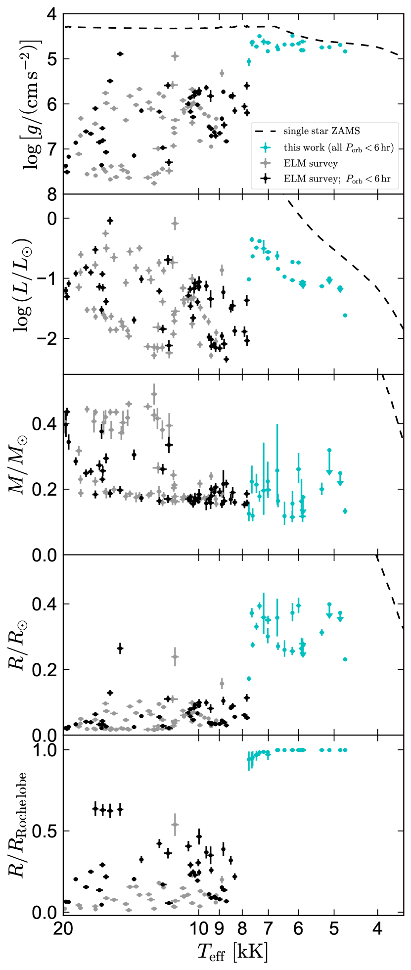
Figure 11: Comparison of objects in our spectroscopic sample (cyan) to WDs and ELM WDs discovered by the ELM survey. Black point show ELM survey targets with $P_{\rm orb}<6$ hours, the period range investigated by our survey. Gray points show longer periods. Our targets have cooler temperatures, lower surface gravities, larger radii, and larger Roche lobe filling factors than the ELM survey targets.

We can now put the proto-ELM WDs in our sample in the context of fully-fledged ELM WDs. Figure 11 compares the 21 objects from our spectroscopic sample with the objects discovered by the ELM survey. Parameters for these objects were taken from Brown et al. (2020). We plot all objects classified as WDs, including some with estimated masses above the $0.3M_{\odot}$ threshold Brown et al. (2020) used to distinguish ELMs from normal WDs. We also separate “short” period binaries with $P_{\rm orb}<6$ (the threshold used in our selection) and binaries with longer periods. For reference, we also plot the zero-age main sequence for single stars with solar metallicity, which is taken from MIST models (Choi et al., 2016).

The top panel shows surface gravity. For the ELM survey, this is measured spectroscopically; for our sample, it is calculated from our mass and radius constraints. The objects in our sample and those from the ELM survey occupy opposite, essentially non-overlapping regions of $T_{\rm eff}-\log g$ space: our candidates have $T_{\rm eff}\lesssim 8,000\,\rm K$ and $\log g\lesssim 5$, while the ELM survey candidates have $T_{\rm eff}\gtrsim 8,000\,\rm K$ and $\log g\gtrsim 5$. This is in some sense by design, since the color selection adopted by the ELM survey was not intended to be sensitive to cooler temperatures. In color-color space, most of our targets overlap with the (more numerous) populations of main-sequence A and F stars, but Gaia distances place them below the main sequence.

The luminosities (2nd panel), radii (4th panel), and Roche lobe filling factors (bottom panel) of objects in our sample are all larger than those of typical objects from the ELM survey. Indeed, none of the ELM survey systems have large enough Roche lobe filling factors that one would expect them to have large enough ellipsoidal variability amplitude to enter our sample (e.g., left panel of Figure 10). Figure 11 shows an apparently strong dichotomy in $R/R_{\rm Roche\,lobe}$ between our sample and the ELM survey objects, but we caution that this is at least partly a selection effect, since objects that do not nearly fill their Roche lobes would not pass our selection criteria.

The masses of the proto WDs in our sample (3rd panel of Figure 11) appear, for the most part, to be an extension of the low-mass mode of the ELM survey’s mass distribution to lower temperatures; they are all consistent with being between 0.1 and $0.25\,M_{\odot}$. We note that our masses are constrained dynamically from the measure radii and ellipsoidal variability amplitudes, while the masses of the ELM survey objects are measured by comparing measurements of $T_{\rm eff}$ and $\log g$ to evolutionary models. It is not obvious that either of these approaches is better, but their limitations are different.

The mass distribution of the ELM survey sample is bimodal, with one mode at $M\lesssim 0.2\,M_{\odot}$ and one at $M\gtrsim 0.4M_{\odot}$. This has been interpreted as a consequence of CNO flashes experience by intermediate mass He WDs, which have been predicted to accelerate their evolution (e.g. van Kerkwijk et al., 2005; Brown et al., 2016). However, the lifetimes of low-mass proto-WDs appear to decrease monotonically with WD mass (e.g. Istrate et al., 2014), so the full explanation may be more complicated. In any case, all the objects in our sample seem to have masses more consistent with the lower-mass population. We discuss the mass distribution further in Section 5.

The median mass we infer for the WD companions is $0.81M_{\odot}$, with a dispersion of $0.18M_{\odot}$. This is similar to the mass distribution inferred from companions to WDs from the ELM survey, which has a mean of $0.76M_{\odot}$ and a dispersion of $0.25M_{\odot}$ (Brown et al., 2016). It is also similar to the mass distribution of WDs in normal CVs, which has mean value of $0.83M_{\odot}$ and a dispersion of $0.23M_{\odot}$ (e.g. Zorotovic et al., 2011; Pala et al., 2020). All of these values are larger than the mean mass observed for isolated WDs, which is about $0.64M_{\odot}$ (Falcon et al., 2010).

From the inferred masses of the proto-WDs and companions, we find gravitational radiation inspiral times ranging from 0.5 to 10 Gyr, with a median of 2.2 Gyr. That is, systems similar to those in our sample have had ample opportunities to reach the period minimum and/or merge. The actual inspiral times are likely shorter for the still-mass transferring systems, since magnetic braking likely still accelerates the angular momentum loss in these systems.

4.2 Moving On: the CV-to-ELM transition

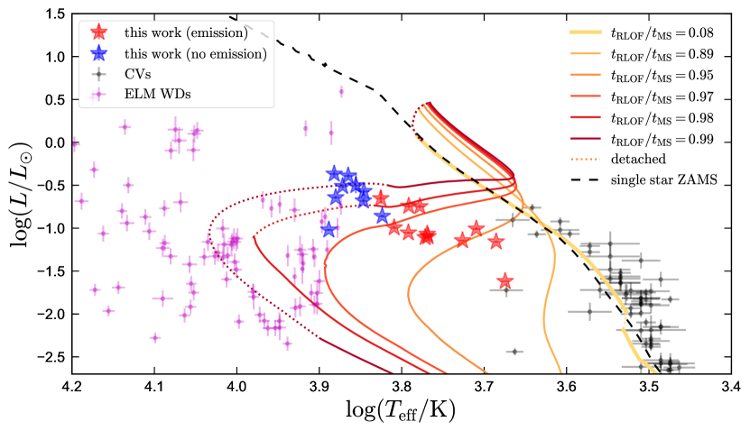
Figure 12: HR diagram. Blue and red stars show targets from our spectroscopic sample with emission lines (likely still mass-transferring) and without them (likely detached). Magenta points show ELM WD candidates from the literature, and gray points show known CV donors, most of which fall close to the main sequence (dashed black line). Colored lines show evolutionary tracks for donor stars in CVs, with the thick yellow line corresponding to an unevolved CV donor, and darker tracks to models in which mass transfer begins increasingly near the end of the main sequence. Dotted lines are detached; solid lines have ongoing mass transfer. Objects in our sample are transitional between CV donors and ELM WDs.

Figure 12 compares, on the HR diagram, the proto-WDs in our sample to known ELM WDs from the compilation of Pelisoli & Vos (2019) (a majority of which are also from the ELM survey) and to known cataclysmic variable donors from Knigge (2006). These samples are described in more detail in El-Badry et al. (2021b). We also show MESA binary evolution models (Paxton et al., 2011; Paxton et al., 2013, 2015, 2018, 2019) calculated by El-Badry et al. (2021b), which show the evolution of an initially $1.1M_{\odot}$ donor that begins transferring mass to a $0.9M_{\odot}$ WD at various points in its evolution. The $t_{\rm RLOF}/t_{\rm MS}$ values noted in the legend indicate the fraction of the donor star’s normal main-sequence lifetime that has elapsed when mass transfer begins. The yellow track shows a model in which mass transfer begins before the donor has undergone significant nuclear evolution – the most common scenario for CVs. In this case, the donor stays close to the main sequence as it shrinks. The other tracks show models in which mass transfer begins near the end of the donor’s main sequence evolution, with darker colors corresponding to progressively more evolved donors. The most evolved models eventually become detached (dotted lines).

The donors in our spectroscopic sample fall between the CV donors and the literature ELM WDs, in a region of the HR diagram that is spanned by the set of MESA models we show. The transition between objects with and without emission lines in our sample occurs at a similar effective temperature as detachment in the MESA models. In the models, detachment occurs when the donor loses its convective envelope and magnetic braking becomes inefficient, slowing the inspiral of the binary. This typically occurs a temperatures between 6,500 and 7,000 K. In the model with $t_{\rm RLOF}/t_{\rm MS}=0.95$, the binary has reached sufficiently short periods ($\sim$2 hours) when the donor loses its convective envelope that angular momentum losses from gravitational waves are sufficient to keep the system in Roche lobe contact.

The basic picture of detachment occurring at temperatures where magnetic braking becomes inefficient seems to be supported by the observed systems. The transition from mass-transferring CVs to detached ELMs is then related to the Kraft break (Kraft, 1967); i.e., the abrupt change in typical rotation periods of main sequence stars at effective temperatures near 6,500 K. This break is thought to occur because stars warmer than this lack convective envelopes and thus cannot generate a magnetic field at the boundary between the convective and radiative layers. This makes removal of spin angular momentum (and orbital angular momentum, in tidally synchronized binaries) via magnetic braking inefficient. The details of this picture are somewhat murky, because significant magnetic fields are observed to exist in stars without radiative/convective boundaries (e.g. Donati & Landstreet, 2009). However, the existence of the Kraft break provides good empirical evidence that magnetic braking is less efficient above $T_{\rm eff}\approx 6,500\,\rm K$, and the mass transferring-to-detached transition we observe likely occurs through a similar process. The exact temperature threshold at which donors in our sample become detached is still unclear, because faint disks may not lead to detectable emission lines. One object with $T_{\rm eff}\approx 6,662\,\rm K$ (P_3.13a) has no emission lines but shows clear light curve evolution suggestive of a disk; another, with $T_{\rm eff}\approx 7,022\,\rm K$ (P_3.21a) shows more tentative evidence of evolution (Appendix C).

4.2.1 Are sdA stars evolved CVs?

There are three objects, plotted in magenta in Figure 12, that appear to have similar effective temperatures and higher luminosities than the warmest objects in our sample. These targets, which are clustered near $\log\left(T_{{\rm eff}}/{\rm K}\right)=3.9$ and $\log\left(L/L_{\odot}\right)=0.5$, are “sdA” stars identified as “probable” proto-ELM WDs by Pelisoli et al. (2018). We think it is unlikely, however, that these are the same type of objects in our sample.

The IDs of these objects, as named by Pelisoli et al. (2018), are J0455-0432, J0904+0343, and J1626+1622. Their reported velocity semi-amplitudes are $60\pm 23$, $48\pm 2$, and $93\pm 19\,\rm km\,s^{-1}$. These all correspond to mass functions below $0.03M_{\odot}$, much lower than any of the targets in our sample (Table 3). Inspecting the ZTF light curves of these targets, we do not find evidence of ellipsoidal variability (or other variability with amplitude $\gtrsim$0.01 mag). For the object J0455-0432, the reported $\log g$ and orbital period are inconsistent with a normal WD companion, because in this scenario the proto-WD would not fit inside its Roche lobe. The other two objects have longer orbital periods – so it is possible that a WD companion might escape photometric detection – but it seems unlikely that the orbits of all three objects would be nearly face on, as would be required for the low mass functions to be normal WDs.

Indeed, of the 15 sdA stars classified as confirmed and probable proto-ELM WDs by Pelisoli et al. (2018), just 3 have mass functions above $0.05\,M_{\odot}$. Those that do have mass functions suggestive of normal-mass WD companions have orbital periods longer than 8 hours and, based on their light curves, are not close to Roche lobe filling. This same appears to be true for the larger sample of sdA proto-ELM candidates produced by Pelisoli et al. (2019), of which only 1 of 50 presented large-amplitude ellipsoidal variation (see El-Badry et al., 2021b). We therefore conclude that most sdA stars identified thus far from spectroscopic surveys are not the same class of objects in our sample.

4.3 Comparison to other evolved CVs

Most of the CVs from the literature plotted in Figure 12 have temperatures and spectral types only modestly different from those of main-sequence stars of similar mass. However, there are by now about a dozen CVs that have been proposed to have evolved donors, which are warmer than prescribed by the CV donor sequence at their orbital period.

In Figure 13, we compare the objects in our sample to these objects, and to the canonical donor sequence for unevolved donors (black dashed line). The other objects are QZ Ser (Thorstensen et al., 2002a), EI Psc (also called 1RXS J232953.9+062814; Thorstensen et al. 2002b), SDSS J170213.26 + 322954.1 (Littlefair et al., 2006), BF Eridani (Neustroev & Zharikov, 2008), CSS J134052.0 + 151341 (Thorstensen, 2013), HS 0218+3229 (Rodríguez-Gil et al., 2009), SDSS J001153.08-064739.2 (Rebassa-Mansergas et al., 2014), ASAS-SN 13cl (Thorstensen, 2015), ASAS-SN 15cm (Thorstensen et al., 2016), ASAS-SN 14ho (Gasque et al., 2019), V1460 Her (Ashley et al., 2020), and ASAS-SN 18aan (Wakamatsu et al., 2021). To our knowledge, this represents a near-complete inventory of currently known evolved CV donors, though new systems are regularly being discovered. EI Psc and QZ Ser, two of the first CVs discovered to have unusually evolved donors, were also included in the Knigge (2006) sample plotted in Figure 12; they are the two discrepantly warm objects at low luminosity.

A majority of the objects in our sample, including those that have emission lines and thus are likely still undergoing mass transfer, are hotter than any previously known CV donors. The hottest 8 objects, which have $T_{\rm eff}>7000\,\rm K$, do not have emission lines that are detectable in our spectra. This suggests that they either are fully detached, or are undergoing mass transfer at an even lower rate than the objects with emission lines.

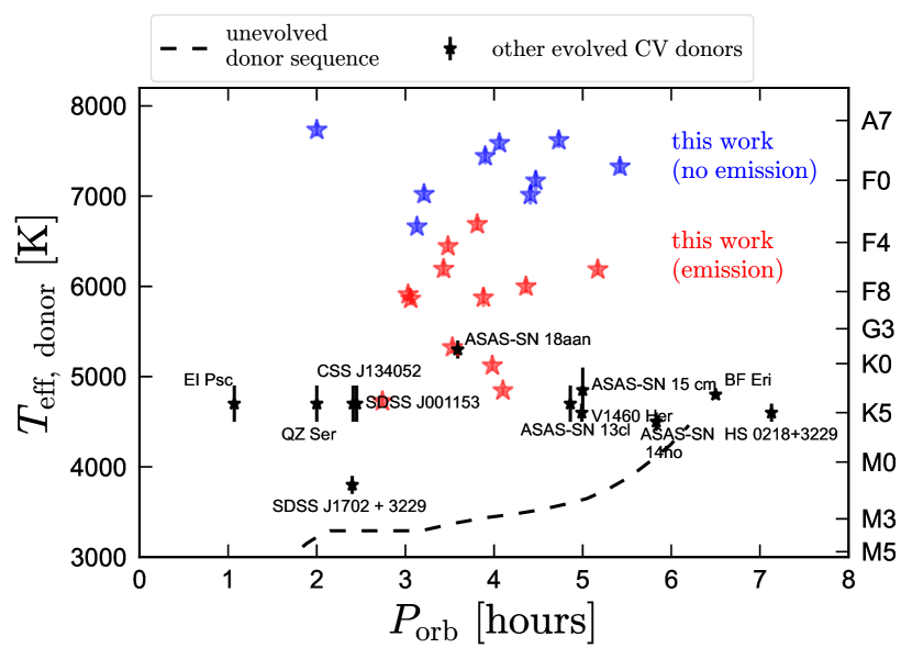
Figure 13: Donor effective temperature versus orbital period. Objects from this study with (red) and without (blue) emission lines are shown with colored stars. Previously known CVs suspected to have evolved donors are shown in black and labeled. Dashed line shows the semi-empirical CV donor sequence from Knigge (2006), along which most normal CV donors are found. Most of the objects in our sample are hotter than any previously known CV donors. Objects with $T_{\rm eff}<7,000\,\rm K$ have emission lines and likely are still undergoing mass transfer; those with higher temperatures do not.

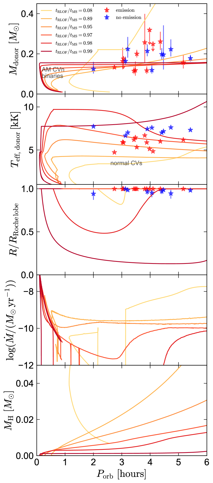
Figure 14: Comparison of our observed targets (red and blue) to MESA binary evolution models for evolved CVs. These are the same models shown in Figure 12. As a function of orbital period, we show the donor mass, effective temperature, Roche lobe filling factor, mass loss rate, and remaining hydrogen mass. The models predict that evolved CV donors at these periods should have masses between 0.1 and $0.2M_{\odot}$, low mass transfer rates compared to normal CVS, and at most a few $\times\,0.01\,M_{\odot}$ of hydrogen remaining.

4.4 Evolutionary history

To gain additional insight into the formation history and future evolution of the systems in our sample, we plot additional properties of the MESA models shown in Figure 12 in Figure 14, now as a function of orbital period.

Compared to normal CVs, models for evolved CVs evolve to much shorter minimum periods, eventually reaching periods between 5 and 30 minutes, where they could be observed as AM CVn binaries (e.g. Podsiadlowski et al., 2003). At the orbital periods represented in our sample, $2<P_{\rm orb}/{\rm hr}<6$, all models that match the temperatures of the observed systems have masses $0.1<M_{\rm proto\,WD}/M_{\odot}<0.2$.

The observed effective temperatures are best matched by models with $0.9<t_{\rm RLOF}/t_{\rm MS}<1$; this depends only weakly on the initial mass of the donor. For all evolved models, the mass transfer rates at periods of 3.1 to 6 hours (above the period gap for normal CVs) are much lower than in normal CVs; this is probably why the emission lines observed in our sample are weaker than in normal CVs and outbursts are less frequent.

The unevolved CV model (yellow, with $t_{\rm RLOF}/t_{\rm MS}=0.08$) becomes detached at orbital periods $2.1\lesssim P_{\rm orb}/{\rm hr}<3.1$. This is the classical “period gap”, which is thought to occur when the donor becomes fully convective and magnetic braking becomes inefficient (e.g. Spruit & Ritter, 1983). The evolved models, however, do not generically become detached at these periods: because they are mostly helium, they do not become fully convective. Within our spectroscopic sample, there are 3 objects with evidence of mass transfer and $2.1\lesssim P_{\rm orb}/{\rm hr}<3.1$. The sample without spectroscopic follow-up contains another 9 systems in this period range; based on their colors and light curves, at least 7 of them are likely mass transferring.

The bottom panel of Figure 14 shows the total remaining hydrogen mass of the donor in the MESA models. Typical values for evolved donors that have not yet reached the WD cooling track (i.e., those that are still evolving toward higher $T_{\rm eff}$) are in the range of $0.003<M_{\rm H}/M_{\odot}<0.03$. The hotter, more evolved donors are predicted to have lower H masses. These values are high enough that spectra would show strong hydrogen features above the period minimum. Below the period minimum, the predicted H masses drop below $10^{-10}M_{\odot}$, where no hydrogen features would be likely to be detected. The H envelope masses also set the lifetime of the bloated proto-ELM WD phase, since objects with large H envelopes can sustain shell burning longer (e.g. Istrate et al., 2014).

5 Discussion

5.1 Donor masses

The distribution of donor masses found in our fitting is relatively narrow, with most systems having best-fit donor masses between $0.1$ and $0.2\,M_{\odot}$ and a few having best-fit masses between $0.2$ and $0.3\,M_{\odot}$. Our MESA evolutionary models (Figure 14) predict that all CV donors sufficiently evolved to reach $T_{\rm eff}\gtrsim 4,500$ K at $P_{\rm orb}\lesssim 6$ hours should have masses lower than $\approx 0.2\,M_{\odot}$, with the most common donor mass being about $0.15M_{\odot}$.

The dispersion in inferred donor masses is somewhat larger than expected from our MESA models. In particular, several objects have inferred masses $M>0.2M_{\odot}$, larger at the $2\sigma$ level than predictions of any of the models. The most banal explanation would be that these objects simply have slightly overestimated masses. As described in Section 3.4.1, this could occur if an accretion disk contributed significantly to the SED, leading to an overestimate of the angular diameter, and hence, the radius and mass. Such unaccounted-for contributions from the disk are more likely to affect systems with detected emission lines (red points in Figure 14). The few systems with the highest best-fit masses indeed show evidence of a disk in both their spectra and light curves; for these, it seems quite plausible that the best-fit masses could be overestimated.

However, there are also a few systems that do not show emission lines and are more massive than predicted by the MESA models. The most significant cases are P_3.90a ($M_{\rm proto\,WD}=0.21\pm 0.03M_{\odot}$) and P_4.73a ($M_{\rm proto\,WD}=0.20_{-0.02}^{+0.03}M_{\odot}$). We now explore whether such masses can be reconciled with the evolutionary scenario of recently detached evolved CVs.

5.1.1 How robust are the model predictions for proto-WD masses ?

To investigate the sensitivity of donor masses in the MESA calculations to the input physics and initial parameters of the component stars, we varied the MESA calculations from those described in El-Badry et al. (2021b) in the following ways:

1. Increase the initial donor mass from $1.1M_{\odot}$ to $1.5M_{\odot}$.

2. Decreasing the initial metallicity from $Z=0.02$ to $Z=0.001$.

3. Increasing the exponential overshooting parameter from $f_{\rm ov}=0.014$ to 0.028.

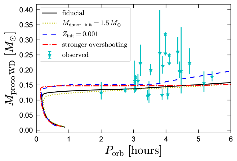
Figure 15: Comparison of observed proto-WDs to MESA calculations with a range of initial conditions and input physics. All model calculations have initial periods chosen such that Roche lobe overflow begins just before the end of the donor’s main-sequence evolution ($t_{\rm RLOF}/t_{\rm MS}\approx 0.98$). The predicted proto-WD masses at these periods depend only weakly on modeling assumptions, as they are set primary by the core-mass vs radius relation for objects with degenerate cores.

In all calculations (including the fiducial model, which is the one labeled $t_{\rm RLOF}/t_{\rm MS}=0.97$ in Figures 12 and 14), we fine-tune the initial period such that the secondary first overflows its Roche lobe at $\approx 97\%$ of its main sequence lifetime.The results of these experiments are shown in Figure 15. Increasing the initial donor mass has basically no effect on the mass that remains when the binary reaches $P_{\rm orb}$ < 6 hours. Increasing the size of the overshooting region and decreasing the initial metallicity both slightly increase the mass of the core that survives at short periods, but the difference is quite modest, only $\sim 0.02M_{\odot}$ at fixed period. Varying other parameters, such as the mass of the accreting WD or the convective mixing length (“$\alpha$”) have similarly small effects.

For WD + MS binaries above the bifurcation limit (i.e., those with initial separations wide enough that mass transfer begins as the donor ascends the giant branch; see Podsiadlowski et al. 2003) that go through stable mass transfer, the relationship between final orbital period and WD mass is reasonably well understood (e.g. Rappaport et al., 1995). In such systems, the orbit expands as the donor loses mass, so the final separation is set by the maximum radius of a giant with a given degenerate core mass. For our systems, which are below the bifurcation limit, the relation is somewhat less clear, because there need not necessarily be a simple relation between core mass and radius. Nevertheless, our calculations do suggest the dispersion in donor mass at fixed period should be small for binaries formed through stable mass transfer. Calculations by other authors (e.g. Lin et al., 2011; Chen et al., 2017; Li et al., 2019) find similar masses, all in the range of 0.14 to 0.18, for low-mass white dwarfs formed by stable mass transfer with $P_{\rm orb}\lesssim 6$ hours.

5.1.2 Could the more massive proto-WDs have formed via common envelope ejection?

It is also worth considering whether the overmassive, already-detached systems in our sample could have formed via common-envelope evolution (CEE; which likely allows a significantly wider range of proto-WD masses at these periods; e.g. Li et al. 2019) rather than stable mass transfer. Systems which begin mass transfer on the giant branch with donor masses that are initially significantly larger than the mass of the accreting WD have too-high accretion rates to sustain stable mass transfer and instead spiral to short periods through a common envelope phase. It has been argued (e.g. Brown et al., 2016) that a dominant fraction of all low-mass WDs form through this channel and only become detached at short ($P_{\rm orb}\lesssim 1\,\rm hour$) periods. The details of what occurs during CEE are not well understood, and so it is commonly invoked to explain the existence of ELM WDs whose properties cannot be easily explained by stable mass transfer. At periods of a few hours, the mass distribution of WDs from the ELM survey suggests that perhaps half of the observed systems formed via stable mass transfer and the rest formed through CEE (e.g. Li et al., 2019).

It is unclear whether a proto-WD formed through CEE might spend an appreciable amount of time nearly Roche lobe filling, or whether enough of the proto-WD’s envelope is ejected during CEE that the proto-WD is expected to emerge already having shrunk well inside its Roche lobe. However, there are other cases in the literature where CEE is assumed to have occurred and the filling factor is still large (e.g. Irrgang et al., 2021). Formation through CEE would likely also allow for a wider range of envelope masses (and thus effective temperatures) during the proto-WD phase (Calcaferro et al., 2018).

5.2 Selection function, space density, and birth rate

For population modeling, it will be important to know what fraction of evolved CV-like objects that our survey is sensitive to. As described in Section 2, there are several conditions that must be met for an evolved CV to enter our spectroscopic sample:

1. The object must appear in the Gaia catalog. This should not significantly affect the selection function, because Gaia eDR3 is basically complete down to our magnitude limit of $G<18$ (e.g. Boubert & Everall, 2020; Fabricius et al., 2021; Gaia Collaboration et al., 2021a), except in very crowded regions.

2. Apparent magnitude $G<18$. For typical objects in the spectroscopic sample with $M_{\rm G}\approx 7$, this corresponds to a distance limit of 1.6 kpc, neglecting extinction. The limit is, however, fuzzy, both because our sample contains objects with a range of absolute magnitudes, and because extinction varies with sky position and distance.

3. Fractional parallax uncertainty better than 20% (i.e., parallax_over_error > 5). For a star with $G=18$, the typical reported parallax uncertainty in Gaia eDR3 is $\sigma_{\varpi}=0.120\,\rm mas$. For $G=16$, it is $0.042\,\rm mas$ (Lindegren et al., 2021a).

   From the mean parallax uncertainty as a function of apparent magnitude, one can calculate the expected parallax_over_error for a source of given absolute magnitude as a function of distance (e.g. El-Badry et al., 2019; Rix et al., 2021). For sources with $M_{\rm G}\gtrsim 6.5$, the cut of parallax_over_error > 5 has no significant effect on the selection function, because most such sources will automatically pass the cut if they have $G<18$. For intrinsically brighter sources (of which our sample contains only a few), the cut can become relevant. For example, at $M_{\rm G}=5$ (brighter than any source in our sample), a cut of $G<18$ corresponds to a distance limit of $\approx 4$ kpc, but parallax_over_error > 5 corresponds to a limit of $\approx 2.6$ kpc.

4. CMD position well below the main sequence: we only considered targets whose observed magnitudes (without extinction correction) place them below a crude cut in color – absolute magnitude space (Figure 1). Our final light-curve selected sample (unlike the parent sample) does not hug the dividing line at the upper edge of the selection region. This suggests that our selection probably does not exclude a large fraction of similar systems, but extending the search region closer to the main sequence is needed to confirm this. In the absence of disk contamination, our MESA models suggest that systems with the most evolved donors reach higher temperatures and thus move farther blueward of the main sequence (Figure 12). Like the magnitude limit, our CMD selection introduces a bias against systems with high extinction. However, the reddening vector in the Gaia CMD is nearly parallel to the selection region boundary (Figure 1), so this effect is modest.

5. Good ZTF light curve: Requirement of a ZTF light curve limits the sample to declination $\delta\gtrsim-28$ deg. This cut removed $\approx 40\%$ of sources passing the cuts above. Basically all sources with uncontaminated photometry within the ZTF footprint have light curves, but as of DR4, approximately $12\%$ of candidates had fewer than 40 uncontaminated epochs and therefore were not included in our sample. Requiring a good ZTF light curve thus removes $\approx 50\%$ of otherwise acceptable sources.

6. “Well behaved” ellipsoidal light curve with peak-to-peak variability amplitude >15%. For systems that are Roche lobe filling, this amplitude limit corresponds to an inclination limit of $\sin i\gtrsim 0.5$, or $i\gtrsim 45$ degrees. For a $\sin i$ inclination distribution, this excludes 29% of binaries. For recently detached systems, the fraction of binaries we can expect to detect depends on the Roche lobe filling factor (Figure 10). We should not expect to detect any systems with filling factors less than 0.8. For filling factors of 0.9, we expect to detect only systems with $i\gtrsim 65$ degrees, or about 42% of systems.

   The “well-behaved” requirement is more difficult to quantify. Our search would not be sensitive to CVs with large-amplitude, irregular, and frequent brightness variations, as are frequently observed in normal CVs and several related classes of compact binaries (e.g., bottom left and center panels of Figure 2). Such variability would likely thwart our period search. On the other hand, occasional outbursts that occur on top of an otherwise periodic light curve (e.g. Figure 6) or modest changes in the mean magnitude due to changes in disk structure (e.g. Figure 5) do not prevent sources from being detected. Fortunately, most evolved CVs at $P_{\rm orb}<6$ hours are expected to have low accretion rates, and thus, faint disks and infrequent outbursts. We therefore expect most evolved CVs, and all proto-ELM WDs that recently become detached, to have well-behaved light curves to which our search is sensitive.

7. Spectroscopic follow-up: We have thus far obtained multi-epoch spectra for 21 of 51 light-curve selected targets. The objects we followed-up are biased somewhat toward bright absolute magnitudes: the spectroscopic sample includes only one object with $M_{\rm G}>8$, while the full sample includes 13. For objects with $M_{\rm G}<8$, the $M_{\rm G}$ distribution of the spectroscopic sample is representative of that of the full light-curve selected sample; there, we have observed 53% of all objects.

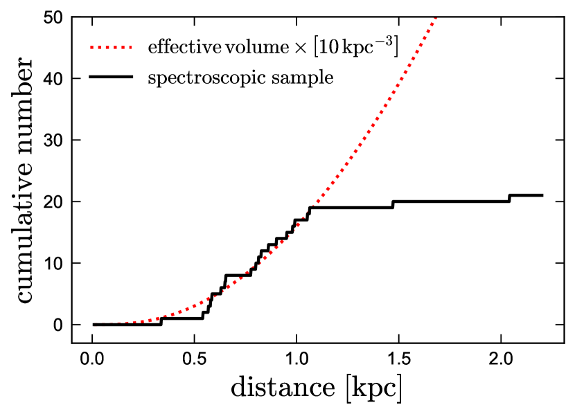
Figure 16: Dotted red line is proportional to the effective stellar volume contained in a sphere of given radius, accounting for the exponential vertical density structure of the Galactic disk (Equation 13). Black line shows the cumulative distance distribution of our spectroscopic sample. A space density of $10\,\rm kpc^{-3}$ makes these roughly agree within 1 kpc, beyond which they strongly diverge. This suggests that within 1 kpc, the completeness of our sample does not decrease much with distance. The true space density is about 6 times larger, $\sim 60\,\rm kpc^{-3}$, because we are not sensitive to all systems and have not spectroscopically followed-up all objects.

5.2.1 Space density

As a simple diagnostic of how the survey’s completeness varies with distance, we compare in Figure 16 the cumulative distance distribution of sources in the spectroscopic sample to the effective stellar volume enclosed in a given distance limit. We define the latter as the expected number of stars in a sphere of radius $d_{\rm max}$ divided by the stellar density at the disk midplane:

$$\tilde{V}=2\pi\int_{0}^{d_{{\rm max}}}e^{-z/h_{z}}\left(d_{{\rm max}}^{2}-z^{2}\right)dz\\$$ (13)

where $h_{z}=0.3\,\rm kpc$ is the disk scale height and $z$ the vertical coordinate. This expression asymptotes to $4\pi d_{\rm max}^{3}/3$ in the limit of $d_{\rm max}\ll h_{z}$; otherwise, it “corrects” for the decreasing density above and below the disk at large $d_{\rm max}$.

Figure 16 shows that the number of objects in our spectroscopic sample approximately tracks Equation 13 out to $\approx 1$ kpc when we scale it by an assumed midplane space density of $10\,\rm kpc^{-3}$. This suggests that the completeness is relatively constant out to this distance, and then drops precipitously. Accounting for the objects that fail to enter our sample because of lack of good light curves ($\sim$ 50%), incomplete spectroscopic follow-up ($\sim$ 50%), and low inclination ($\sim$ 30%) suggests that about 1 out of 6 evolved CVs and proto WDs with $8\lesssim M_{G}\lesssim 5$ enters our sample, and thus that the true space density is about $60\,\rm kpc^{-3}$. This estimate of course brushes over many complexities of the selection function; we defer more detailed modeling to future work. For context, $60\,\rm kpc^{-3}$ is a factor of 2.7–5 lower than the space density of ELM WDs discovered by the ELM survey (160-300 in the same units; Brown et al., 2016), about a factor of 80 lower than the space density of CVs ($4800\pm 800$; Pala et al., 2020), about 8 times lower than the space density of AM-CVn binaries ($500\pm 300$; Carter et al., 2013), and 75,000 times lower than the space density of all WDs ($(4.49\pm 0.38)\times 10^{6}$; Hollands et al., 2018).

5.2.2 Birth Rate

Evolutionary interpretation of these densities depends critically on the lifetime of the proto-ELM phase, and on the lifetimes of other types of binaries to which they are linked. Our MESA models predict observable lifetimes ranging from 200 Myr to 2 Gyr. More-evolved models that become detached have longer lifetimes than less-evolved models that do not, because magnetic braking accelerates the evolution of the less-evolved models. We adopt $\tau=500\,\rm Myr$ as a typical lifetime in estimating the birth rate.

To convert the measured space density to a birth rate, we first estimate the total number of evolved CVs and proto-ELM WDs in the Milky Way. We model the Milky Way as an exponential disk with vertical scale height $h_{z}=0.3\,\rm kpc$ and radial scale length $h_{R}=3\,\rm kpc$. This yields a total number

$$N_{{\rm tot}} =n_{0}\int_{0}^{2\pi}\int_{-\infty}^{{\rm\infty}}\int_{0}^{\infty}\exp\left(-\frac{R-R_{{\rm Sun}}}{h_{R}}-\frac{\left|z\right|}{h_{z}}\right)R\,{\rm d}R\,{\rm d}z\,{\rm d}\phi$$ (14)

$$=4\pi n_{0}h_{z}h_{R}^{2}\exp\left[R_{{\rm Sun}}/h_{R}\right]$$ (15)

$$\approx 488\,{\rm kpc^{3}\times}n_{0}.$$ (16)

Here $n_{0}=60\,\rm kpc^{-3}$ is our inferred midplane space density in the solar neighborhood and $R_{\rm Sun}=8\,\rm kpc$ is the distance from the Solar neighborhood to the Galactic center. We then divide the total number of systems by the typical lifetime, $\tau=500\,\rm Myr$, yielding a Milky Way-integrated birth rate of

$$\mathcal{R}_{{\rm Milky\,Way}}=\frac{N_{{\rm tot}}}{\tau}\approx 59\,{\rm Myr}^{-1}.$$ (17)

The uncertainty on this estimate is probably about a factor of 2, with comparable contributions from the uncertainty in the population-averaged lifetime of evolved CVs and from uncertainty in the space density.

This birth rate is a factor of $\sim$ 50 lower than the inferred merger rate for ELM WD binaries, $\mathcal{R}\approx 3,000\,{\rm Myr^{-1}}$ (Brown et al., 2016). This is expected, since the period distribution observed by the ELM survey suggests a large majority of ELM WDs are born at short periods ($P_{\rm orb}\sim 0.5\,\rm hr$) via common envelope ejection and quickly merge. On the other hand, the birth rate of AM CVn binaries is $\mathcal{R}\approx 130\,{\rm Myr^{-1}}$ (Carter et al., 2013; Brown et al., 2016), a factor of 2.2 larger than our inferred birth rate of evolved CVs and consistent with it when plausible uncertainties on both rates are accounted for.

We conclude that the evolved CV channel contributes only a small fraction of all ELM WDs ever formed. However, since ELM WDs formed at short periods via common envelope ejection quickly merge, it contributes a significant fraction of all ELM WD binaries existing at a given time. The similarity between the birth rates of evolved CVs and AM-CVn binaries suggests that the evolved CV channel may contribute significantly to the formation of AM-CVn systems.

6 Conclusions

We have initiated a spectroscopic survey for compact binaries containing a Roche-filling, low-mass proto-white dwarf secondary. These objects fill in the evolutionary gap between evolved CV donors and ELM WDs formed via stable mass transfer.

Our search is sensitive to systems on both sides of the CV-to-ELM WD transition: systems with still-ongoing mass transfer, and systems that are detached WD + proto-ELM WD binaries in which mass transfer has recently ceased. Thus far, we have obtained spectroscopic follow-up of about 40% of all candidates brighter than $G=18$ that satisfy our search criteria. The sample we have assembled is the first systematic sample of its kind. It contains all known systems with donor temperatures above $\sim$5,000 K and triples the number of spectroscopically confirmed evolved CVs. Including systems which have not yet been spectroscopically followed-up (Appendix D), it expands the evolved CV population by a factor of $\sim$6. Our main results are as follows:

1. Target selection: We select targets that fall below the main sequence in the Gaia color-magnitude diagram (Figure 1) and have ZTF light curves dominated by ellipsoidal variation (Figure 4). This selection yields binaries in which the donor star is hotter and more luminous, and the mass transfer rate is lower, than in normal CVs with similar periods. We identified 51 candidates and have obtained multi-epoch spectra for 21 of them. The selection strategy is very efficient: 100% of the sources we have obtained spectra for are indeed evolved CVs or their recently-detached ELM WD descendants. Our final sample is well-separated from related populations of ELM WDs, hot subdwarfs, and normal CV donors in the color-magnitude diagram, constituting a distinct population.

2. Donor properties: Joint analysis of light curves (Figure 4), low-resolution spectra (Figure 7), radial velocities (Figure 8), and broadband spectral energy distributions (Figure 9) allows us to obtain tight constraints on the proto-WD masses, radii, and effective temperatures. Our inferred proto-WD masses are typically quite low, $M_{\rm proto-WD}\approx 0.15\,M_{\odot}$ (Figure 14). The masses of the WD companions are high but typical for CVs, $M_{\rm WD}\approx 0.8M_{\odot}$ on average. These proto-WDs are cooler and more bloated than objects observed by the ELM survey (Figure 11). On the HR diagram, they fall between known populations of “normal” CV donors and detached ELM WDs (Figure 12).

3. Comparison to other CVs: All the donors in our sample are significantly warmer than typical CV donors at the same orbital period, and most of them are warmer than any previously characterized evolved CVs (Figure 13). Without a well-informed prior or multi-epoch spectroscopy, the objects in our sample likely would not have been characterized as CVs at all, because most have not been observed in outburst and only show weak emission lines.

4. Mass transfer rates: More than half of the systems have ongoing mass transfer, as evidenced by weak emission lines (Figure 7), eclipses of the donor by an accretion disk (Figure 4), and irregular variations in brightness (Figure 5). Only two of the systems with evidence of ongoing accretion exhibit dwarf nova-like outbursts (Figure 6), indicating that the recurrence timescale of such outbursts is long ($\gtrsim 10$ years), if they occur at all. The systems that do not show evidence of ongoing accretion must have terminated mass transfer relatively recently, as their proto-WDs all nearly fill their Roche lobes (Figure 10).

5. Formation histories: Most of the systems in our sample can be well described by binary evolution models in which a relatively massive ($1\lesssim M/M_{\odot}\lesssim 2$) donor overflows its Roche lobe and begins transferring mass to a WD companion near the end of its main-sequence evolution. Mass transfer in these models must begin before the donor star starts to ascend the giant branch (“below the bifurcation period”), or the final orbital period will be too long.

   In these models, the transition from mass-transferring CV to detached ELM WD occurs when the effective temperature of the donor increases to above 6500–7000 K and the donor star loses its radiative envelope. This presumably leads to a weakening, or at least a significant rearrangement, of the donor’s magnetic field, which is thought to originate at the boundary between the radiative and convective layers (e.g. Spruit & Ritter, 1983). This picture is broadly supported by the spectroscopic properties of the donors in our sample: those with $T_{\rm eff}\lesssim 7000\,\rm K$ have emission lines, likely indicative of ongoing mass transfer, and those with hotter temperatures do not (Figure 13).

6. Space density and birth rate: After accounting for the selection function of our survey, we infer a local space density of evolved CVs $n_{0}\sim 60\,\rm kpc^{-3}$ and a Galaxy-integrated formation rate $\mathcal{R}\sim 60\,\rm Myr^{-1}$ (Section 5.2). This birth rate is a factor of $\sim$ 50 lower than the merger rate for ELM WD binaries, likely because a large majority of ELM WDs are born at short periods and quickly merge. It is a factor of $\sim 2.2$ lower than the inferred birth rate of AM CVn binaries.

Objects in our sample are prime candidates to eventually evolve to short periods and become AM CVn binaries (Figure 14), either after a period of detachment (for the most evolved systems), or remaining mass transferring to short periods (less evolved systems; e.g. Figure 12). Previous work from the ELM survey has shown that a majority of ELM WDs do not form AM CVn systems (Brown et al., 2016). However, the extreme mass ratios in our sample (median $M_{\rm proto\,WD}/M_{\rm WD}=0.24$) should make them more likely to evolve to short periods without merging (e.g. Marsh et al., 2004). The fate of extreme mass ratio WD binaries after mass transfer begins remains unclear (e.g. Shen, 2015).

More work is required for a more complete understanding of the evolved CV/proto-ELM WD population. Spectra with higher resolution and SNR from 10m-class telescope will allow us to investigate the nature and phase-dependence of emission lines in the systems with weak emission, and to measure detailed abundance patterns of the donors. HST/COS spectroscopy of the systems that are brightest in the UV will allow us to measure the temperatures of the accreting WDs, yielding constraints on the time-averaged accretion rate. High-cadence photometry will shine light on the origin of the photometric scatter found in the light curves of a majority of the ZTF light curves (Figure 4), which for many sources is still consistent with coming from disk flickering, longer-term changes in disk structure, or pulsations in the donor.

Data Availability

The data underlying this article are available upon reasonable request to the corresponding author. For convenience, we include as supplemental data a digital table that combines all data from Tables 1-5.

Appendix A Roche lobe filling factor prior

In our fitting in Section 3.7, we require a prior on the proto-WD’s Roche lobe filling factor, $f=R_{\rm proto\,WD}/R_{\rm Roche\,lobe}$, which is often strongly covariant with the orbital inclination. One option would be to adopt a uniform prior between $f_{\rm min}$, the minimum filling factor that can explain the observed ellipsoidal variability amplitude, and 1, essentially implying that all allowed filling factors are equally probable. However, our MESA evolutionary models predict that donors contract more slowly when the filling factor is near 1. This suggests that our prior of $f$ should give more weight to value of $f$ near unity.

This is illustrated in Figure 17. The left panel shows the MESA model with $t_{\rm RLOF}/t_{\rm MS}=0.98$, whose effective temperature evolution provides a good match for several objects in our sample, just after it becomes detached. The red line shows the model, and the dotted black line shows a quadratic fit in the form $f=1-at^{2}$, which we use to avoid numerical noise in calculating derivatives. It is clear that $f(t)$ steepens with decreasing $f$, meaning e.g. that the model spends more time contracting from $f=1$ to $f=0.98$ than from $f=0.9$ to $0.88$.

The probability of observing such a binary at a given $f$ is

$$p\left(f\right)=\frac{{\rm d}p}{{\rm d}f}=\frac{{\rm d}p}{{\rm d}t}\frac{{\rm d}t}{{\rm d}f},$$ (18)

where $\frac{{\rm d}p}{{\rm d}t}$ represents the (presumed constant) probability of observing the system per time interval. For $f(t)=1-at^{2}$, this yields

$$p\left(f\right)=\begin{cases}\frac{1}{2\sqrt{\left(f_{\rm min}-1\right)\left(f-1\right)}},&f\geq f_{{\rm min}}\\ 0,&f<f_{{\rm min}}\end{cases},$$ (19)

with no dependence on $a$. Thus, for any $f(t)$ that decrease quadratically near detachment, Equation 19 provides a reasonable approximation for $p(f)$. This is plotted in the middle panel of Figure 17, where we chose $f_{\rm min}=0.8$. The function diverges for $f\to 1$, but its integral converges (right panel). We adopt Equation 19 as our prior on $f$ for all systems which have no clear emission lines and thus appear to be detached.

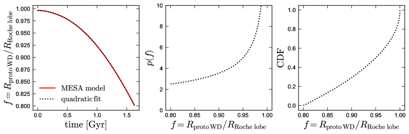
Figure 17: Left: Roche lobe filling factor of the MESA binary model with $t_{\rm RLOF}/t_{\rm MS}=0.98$. Dotted black line shows a quadratic fit, which we use to mitigate numerical noise. The model contracts less steeply just after mass transfer ceases (when $f\approx 1$), and the contraction accelerates over time. This means that the distribution of filling factors for randomly observed detached systems is expected to be weighted toward $f=1$. Middle panel shows the distribution of filling factors expected given the quadratic fit in the left panel and a minimum filling factor of 0.8 (Equation 19). Right panel shows the corresponding cumulative distribution function.

Adoption of this prior has a relatively weak effect on our results; for example, none of the inferred proto-WD masses change by more than $0.02M_{\odot}$ when we instead adopt a flat prior. The change is, however, systematic: in all cases, adopting the prior leads to a higher inferred Roche lobe filling factor, and thus, a lower inferred proto-WD mass.

Appendix B H$\alpha$ emission

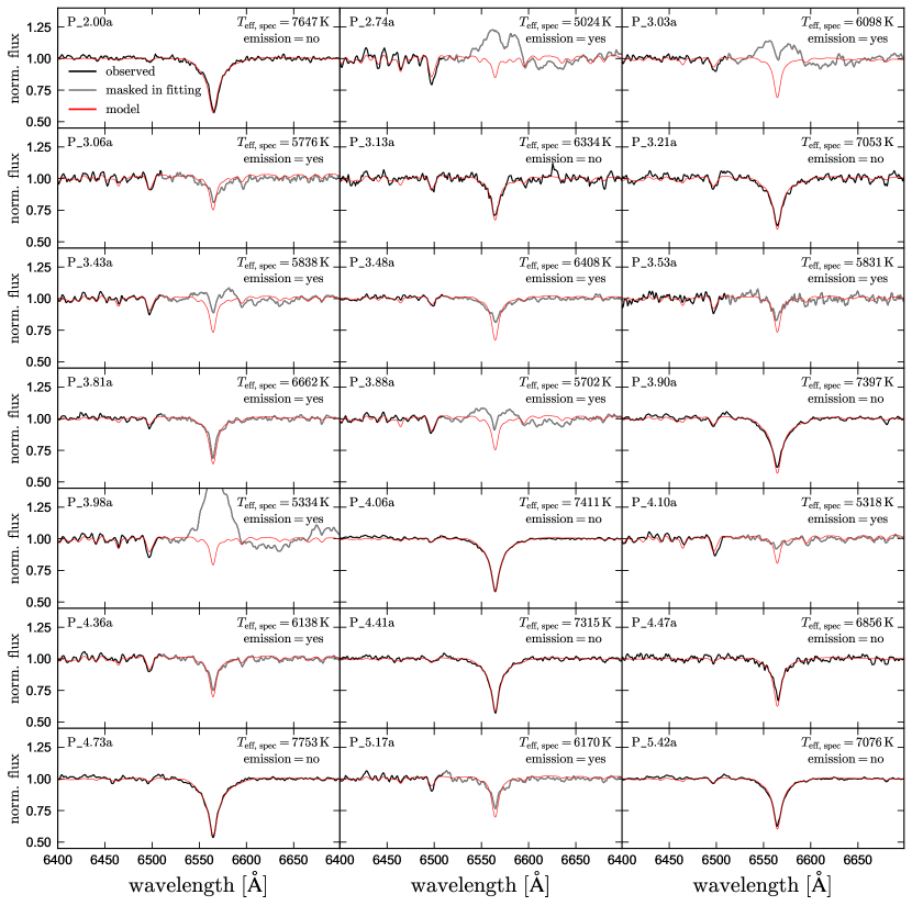
Figure 18: Zoom-in on the H$\alpha$ line for all objects in our spectroscopic sample (full spectra shown in Figure 7). Objects for which the best-fit Kurucz model is significantly deeper than the observed spectrum likely contain H$\alpha$ emission. The model spectrum is fit to the full wavelength range shown in Figure 7.

Figure 18 highlights the H$\alpha$ lines of objects in the spectroscopic sample.

Appendix C Light curve evolution and scatter

To search for long-timescale brightness evolution, we subtracted a Fourier model for the periodic variability from the ZTF $r-$ band light curves. The resulting flux-space residuals are shown in Figure 19 for all objects in the spectroscopic sample. For many sources, this reveals clear evolution in the phase-averaged mean brightness. The source with the most obvious variations is P_3.06a (see Figure 5), with a maximum range of $\sim$7% ($\sim$0.07 mag). Evolution is somewhat more subtle (not accompanied by a clear change in light curve shape) in most other sources, but few-percent variations are common in the sample.

All the sources with clear evolution have donors with $T_{\rm eff}\lesssim 7,000\,\rm K$, consistent with a scenario in which long-term evolution is due to a disk and the hotter donors are detached. There are also several cooler sources that have emission lines and/or eclipses but do not show evolution; these source likely have more stable disks. Two sources (P_3.13a and P_3.21a) show evidence of brightness evolution (only tentative for P_3.21a) but no obvious emission lines.

To assess evolution on shorter timescales, we inspected light curves of the 7 sources in the spectroscopic sample with continuous observations over a few-hour period through the ZTF high-cadence survey. Examples for two sources are shown in Figure 20. Most sources with significant scatter in their full phased light curves have significantly less scatter when only the high-cadence observations are considered (e.g., P_3.98a in Figure 20). One object, P_3.90a, has similar scatter in the high-cadence data and in the full light curve, suggesting the excess variability must occur primarily on short timescales.

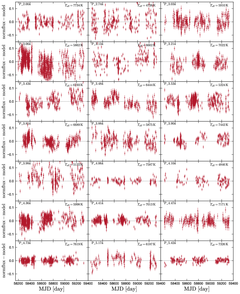
Figure 19: ZTF $r-$band light curves for all objects in the spectroscopic sample, with the mean Fourier model for the full light curve subtracted. About half the light curves (P_3.06a, P_3.13a, P_3.43a, P_3.48a, P_3.81a, P_3.98a, P_4.36a, P_5.17a) show evidence of evolution on long (few months to years) timescales, typically with few-percent changes in brightness.

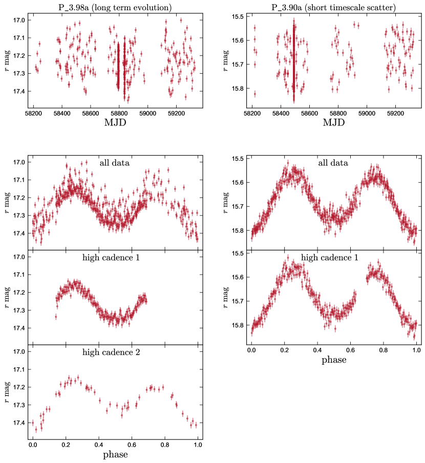
Figure 20: $r-$band light curves for two objects observed by the ZTF high-cadence survey, which provides continuous observations over a few-hour window. Top panels show the full light curves; the high-cadence windows are evident as vertical stripes with many datapoints. Bottom panels show the full phased light curves, as well as phased light curves of only the data taken at high cadence during a single few-hour window. In P_3.98a (left), the scatter within the high-cadence windows is much less (though still nonzero) than in the full light curve, suggesting that most of its scatter is due to longer-timescale disk evolution. The high-cadence light curve also shows evidence of disk flickering. In P_3.90a (right) the scatter in the high-cadence window is similar (about 2%) to that in the full light curve, suggesting it is dominated by short-timescale variations such as pulsations or disk flickering.

Appendix D Light curve-selected targets without spectroscopic follow-up

As described in Section 2, our light curve + CMD selection yielded 51 objects, of which we have thus far spectroscopically followed-up 21. Basic parameters of the objects for which we have not obtained spectra are listed in Table 6, and their ZTF light curves are shown in Figure 21.

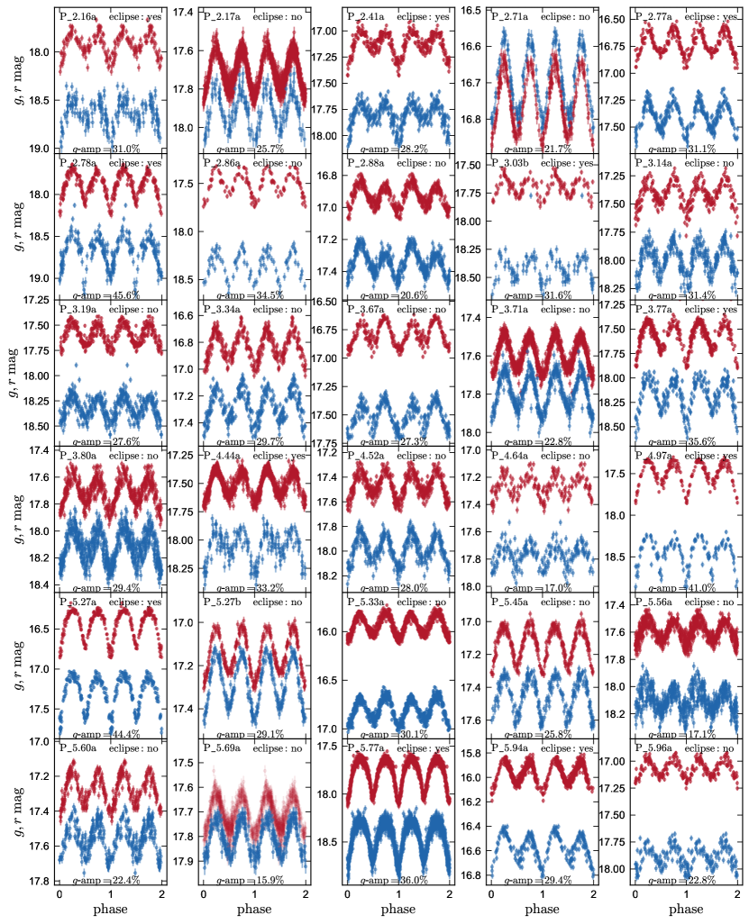
Figure 21: Phased ZTF light curves of the 30 objects identified in our initial sample selection (Section 2) that have not (yet) been followed-up spectroscopically. The sample contains classical ellipsoidal variables, eclipsing systems (presumably with disks), and systems with additional scatter due to long-term evolution and/or pulsations.

Table 6: Objects without spectroscopic follow-up. Parameters are defined as in Table 1.

ID	Gaia eDR3 ID	$l$	$b$	$G$	$P_{\rm orb}$	$\varpi_{\rm corrected}$	$E(g-r)$	$g$-amplitude	$g$-scatter	eclipse?
		[deg]	[deg]	[mag]	[hours]	[mas]	[mag]	[%]	[%]
P_2.16a	6831016738348476800	31.196798	-43.921607	17.98	2.16	$1.81\pm 0.17$	$0.04\pm 0.01$	$31.0\pm 3.1$	6.6	yes
P_2.17a	4086789647048435968	16.841985	-8.809333	17.62	2.17	$0.92\pm 0.13$	$0.15\pm 0.01$	$25.7\pm 1.8$	0	no
P_2.41a	2443219535337313280	96.348334	-67.601219	17.18	2.41	$2.10\pm 0.09$	$0.06\pm 0.02$	$28.2\pm 1.5$	4.8	yes
P_2.71a	3616216816596857984	330.929484	50.744110	16.66	2.71	$0.86\pm 0.08$	$0.00\pm 0.01$	$21.7\pm 0.6$	0	no
P_2.77a	5153771948438163712	198.467868	-59.571062	16.85	2.77	$2.46\pm 0.06$	$0.02\pm 0.01$	$31.1\pm 1.6$	3.7	yes
P_2.78a	6909438962819026560	41.729647	-32.275404	17.89	2.78	$1.71\pm 0.15$	$0.11\pm 0.01$	$45.6\pm 2.3$	7.6	yes
P_2.86a	3652272306837720448	354.915285	52.489703	17.54	2.86	$2.36\pm 0.10$	$0.03\pm 0.01$	$34.5\pm 2.8$	3.8	no
P_2.88a	2859983434955681536	113.362300	-33.515517	16.92	2.88	$1.31\pm 0.08$	$0.04\pm 0.00$	$20.6\pm 0.7$	1.8	no
P_3.03b	4368353340609239936	20.456594	20.691756	17.87	3.03	$1.38\pm 0.13$	$0.38\pm 0.00$	$31.6\pm 5.3$	9.9	yes
P_3.14a	3106121585420422784	214.951623	-1.486974	17.49	3.14	$1.48\pm 0.09$	$0.10\pm 0.02$	$31.4\pm 2.0$	4.9	no
P_3.19a	3373007043559875328	191.954484	4.467368	17.62	3.19	$1.37\pm 0.12$	$0.16\pm 0.04$	$27.6\pm 1.9$	5.9	no
P_3.34a	2467074539612904832	159.793481	-65.773407	16.87	3.34	$1.59\pm 0.07$	$0.00\pm 0.00$	$29.7\pm 1.5$	4.2	no
P_3.67a	2453564290487329280	165.460401	-73.264722	16.97	3.67	$1.82\pm 0.07$	$0.00\pm 0.00$	$27.3\pm 1.2$	3.4	no
P_3.71a	1812627897159845632	62.870714	-13.309963	17.56	3.71	$0.72\pm 0.10$	$0.09\pm 0.01$	$22.8\pm 0.8$	2.0	no
P_3.77a	4223953344655923584	41.618275	-19.079074	17.53	3.77	$0.89\pm 0.12$	$0.15\pm 0.01$	$35.6\pm 7.1$	31.6	yes
P_3.80a	1715477184326927744	117.920994	36.733613	17.87	3.80	$0.72\pm 0.08$	$0.06\pm 0.01$	$29.4\pm 1.2$	4.6	no
P_4.44a	5717210604722373248	234.331125	2.454777	17.63	4.44	$0.88\pm 0.09$	$0.08\pm 0.01$	$33.2\pm 2.3$	4.8	yes
P_4.52a	3325744016547861888	201.735824	-2.770070	17.50	4.52	$1.08\pm 0.10$	$0.14\pm 0.01$	$28.0\pm 1.2$	3.2	no
P_4.64a	3910299549545984000	257.535495	62.412238	17.26	4.64	$1.08\pm 0.11$	$0.03\pm 0.01$	$17.0\pm 2.0$	4.7	no
P_4.97a	1763012778552710528	61.499213	-16.496899	17.60	4.97	$1.49\pm 0.11$	$0.06\pm 0.01$	$41.0\pm 3.3$	6.5	yes
P_5.27a	2477944857025864192	150.912529	-67.405362	16.67	5.27	$1.99\pm 0.37$	$0.00\pm 0.00$	$44.4\pm 1.2$	5.9	yes
P_5.27b	2652639593773429120	65.931043	-49.944372	17.14	5.27	$0.72\pm 0.09$	$0.07\pm 0.01$	$29.1\pm 0.7$	0	no
P_5.33a	2184121338243194624	93.438488	8.305524	16.02	5.33	$2.67\pm 0.03$	$0.04\pm 0.01$	$30.1\pm 0.6$	2.8	no
P_5.45a	3743862209546227584	327.579445	76.471956	17.14	5.45	$0.47\pm 0.07$	$0.00\pm 0.01$	$25.8\pm 1.0$	2.4	no
P_5.56a	997691559644734080	159.807366	19.137537	17.71	5.56	$0.87\pm 0.11$	$0.11\pm 0.01$	$17.1\pm 1.3$	4.7	no
P_5.60a	3740297730288413056	344.568767	71.347303	17.28	5.60	$0.52\pm 0.09$	$0.06\pm 0.04$	$22.4\pm 1.2$	3.5	no
P_5.69a	4241883875351568128	42.892677	-12.409634	17.66	5.69	$0.54\pm 0.09$	$0.14\pm 0.01$	$15.9\pm 0.8$	0	no
P_5.77a	1419776515721297536	80.834579	37.177558	17.86	5.77	$0.88\pm 0.11$	$0.07\pm 0.01$	$36.0\pm 0.7$	4.3	yes
P_5.94a	3035296754374910976	226.832469	3.810814	15.99	5.94	$1.51\pm 0.05$	$0.05\pm 0.02$	$29.4\pm 1.3$	2.5	yes
P_5.96a	3874949971539651840	231.629329	47.310078	17.14	5.96	$1.39\pm 0.10$	$0.00\pm 0.01$	$22.8\pm 1.9$	4.9	no

Appendix E Overlap with other surveys

We cross-matched the 51 light curve-selected candidates with the final sample of low-mass white dwarfs from the ELM survey (Brown et al., 2020). This yielded only one object in common, P_2.71a (J1401-0817 in their catalog). Unlike essentially all other objects discovered by the ELM survey, it has a light curve dominated by large-amplitude ellipsoidal variability, with peak-to-peak amplitude of 28% (see light curve in Appendix D). This suggests that mass transfer only very recently ceased. It is immediately evident from Figure 21 that the object is hotter than any of the other targets in our sample, because it is the only one with $g-r<0$. This explains why most of our targets were not observed by the ELM survey: they are too cool to fall within its color cuts (Brown et al., 2012).

We also cross-matched our sample with the 5,762 ELM WD candidates identified by Pelisoli & Vos (2019). Here too, P_2.71a was the only object that appeared in both samples. This is probably also a consequence of the CMD cuts Pelisoli & Vos (2019) employed, which most of our objects are too red to pass.

We also searched SIMBAD (Wenger et al., 2000) for previous studies of all 51 candidates. Within our spectroscopic sample, this yielded two matches: the object P_2.74a was classified as an eclipsing binary by the LINEAR survey (Palaversa et al., 2013), and P_3.48a was (incorrectly) classified as a Delta Scuti variable by the Catalina survey (Drake et al., 2014).

Several objects in the light curve selected sample without spectroscopic follow-up also had previous classifications: P_2.71a (the same object observed by the ELM survey) was spectroscopically classified as low-mass WD based on its SDSS spectrum by Kepler et al. (2015). P_2.41a was classified as an evolved CV, consistent with our classification, by Rebassa-Mansergas et al. (2014), and was studied in detail. Six objects were classified as eclipsing, contact, or ellipsoidal binaries by the Catalina survey (Drake et al., 2014; Marsh et al., 2017); these are P_5.27a, P_5.27b, P_5.45a, P_5.60a, P_5.77a, and P_5.96a. Given their CMD position, we suspect they are all evolved CVs.

E.1 Known evolved CVs not in our sample

To better understand the selection function of our sample, we also investigated the known evolved CVs that are not among the 51 light curve-selected candidates. We considered all previously known systems in Figure 13 with $T_{\rm eff,\,donor}>4000\,\rm K$. Of the 11 such systems, only SDSS J001153.08-064739.2 (Rebassa-Mansergas et al., 2014) is in our sample (as P_2.41a). Two systems, BF Eri and HS 0218+3229, have orbital periods $P_{\rm orb}>6$ hours, longer than our sample limit. Two systems, V1460 Her and ASAS-SN 13cl, fall outside our selection region in the CMD, as they are closer to the main sequence than the upper limit of our selection region. One system, ASAS-SN 15cm, is fainter than our magnitude limit of $G<18$, and another, ASAS-SN 14ho, is farther south than our declination limit of $\delta>-28$ deg. One object, CSS J134052.0 + 151341, has ellipsoidal variability amplitude less than our limit of $>15\%$, likely because it is almost face-on (Thorstensen 2013 found an inclination of 27 degrees). The last two systems, QZ Ser and EI Psc, were rejected in our light curve search because their ZTF light curves are not dominated by ellipsoidal variation, but show complex and irregular variability. This is likely a consequence of significant changes in the structure of their disks over the $\sim 3$ year ZTF baseline, since their light curves do show ellipsoidal variability over shorter timescales (Thorstensen et al., 2002a, b).

We conclude that while our search strategy should not be expected to find every CV with an evolved donor, it has not missed known objects that we would have expected it to detect. The sensitivity of our search is lowest for objects with high accretion rates, in which the disk contributes significantly to the optical photometry, outbursts are more common, and the light curve is more complicated than expected for simple ellipsoidal variability. At the orbital periods represented in our survey, the accretion rate and light contribution of the disk are expected to be lowest for the most evolved donors (e.g. El-Badry et al., 2021b). This likely explains why most of the systems in our sample are warmer than the previously known systems not included in it (e.g. Figure 13).

References

- Abrahams et al. (2020) Abrahams E. S., Bloom J. S., Mowlavi N., Szkody P., Rix H.-W., Ventura J.-P., Brink T. G., Filippenko A. V., 2020, arXiv e-prints, p. arXiv:2011.12253
- Abril et al. (2020) Abril J., Schmidtobreick L., Ederoclite A., López-Sanjuan C., 2020, MNRAS, 492, L40
- Ashley et al. (2020) Ashley R. P., et al., 2020, MNRAS, 499, 149
- Bailer-Jones et al. (2020) Bailer-Jones C. A. L., Rybizki J., Fouesneau M., Demleitner M., Andrae R., 2020, arXiv e-prints, p. arXiv:2012.05220
- Bellm et al. (2019) Bellm E. C., et al., 2019, PASP, 131, 018002
- Beuermann et al. (1998) Beuermann K., Baraffe I., Kolb U., Weichhold M., 1998, A&A, 339, 518
- Bildsten et al. (2007) Bildsten L., Shen K. J., Weinberg N. N., Nelemans G., 2007, ApJ, 662, L95
- Blackwell & Shallis (1977) Blackwell D. E., Shallis M. J., 1977, MNRAS, 180, 177
- Bohlin et al. (2017) Bohlin R. C., Mészáros S., Fleming S. W., Gordon K. D., Koekemoer A. M., Kovács J., 2017, AJ, 153, 234
- Boubert & Everall (2020) Boubert D., Everall A., 2020, MNRAS, 497, 4246
- Brown et al. (2010) Brown W. R., Kilic M., Allende Prieto C., Kenyon S. J., 2010, ApJ, 723, 1072
- Brown et al. (2012) Brown W. R., Kilic M., Allende Prieto C., Kenyon S. J., 2012, ApJ, 744, 142
- Brown et al. (2016) Brown W. R., Kilic M., Kenyon S. J., Gianninas A., 2016, ApJ, 824, 46
- Brown et al. (2020) Brown W. R., et al., 2020, ApJ, 889, 49
- Calcaferro et al. (2018) Calcaferro L. M., Althaus L. G., Córsico A. H., 2018, A&A, 614, A49
- Cardelli et al. (1989) Cardelli J. A., Clayton G. C., Mathis J. S., 1989, ApJ, 345, 245
- Carter et al. (2013) Carter P. J., et al., 2013, MNRAS, 429, 2143
- Chen et al. (2017) Chen X., Maxted P. F. L., Li J., Han Z., 2017, MNRAS, 467, 1874
- Choi et al. (2016) Choi J., Dotter A., Conroy C., Cantiello M., Paxton B., Johnson B. D., 2016, ApJ, 823, 102
- Cutri et al. (2014) Cutri R. M., et al., 2014, VizieR Online Data Catalog, p. II/328
- Donati & Landstreet (2009) Donati J. F., Landstreet J. D., 2009, ARA&A, 47, 333
- Drake et al. (2009) Drake A. J., et al., 2009, ApJ, 696, 870
- Drake et al. (2014) Drake A. J., et al., 2014, ApJS, 213, 9
- Driebe et al. (1998) Driebe T., Schoenberner D., Bloecker T., Herwig F., 1998, A&A, 339, 123
- Eggleton (1983) Eggleton P. P., 1983, ApJ, 268, 368
- El-Badry et al. (2018) El-Badry K., et al., 2018, MNRAS, 476, 528
- El-Badry et al. (2019) El-Badry K., Rix H.-W., Tian H., Duchêne G., Moe M., 2019, MNRAS, 489, 5822
- El-Badry et al. (2021a) El-Badry K., Rix H.-W., Heintz T. M., 2021a, MNRAS,
- El-Badry et al. (2021b) El-Badry K., et al., 2021b, arXiv e-prints, p. arXiv:2104.07033
- Enenstein et al. (2021) Enenstein J., Burdge K., Prince T., 2021, Research Notes of the American Astronomical Society, 5, 90
- Evans et al. (2018) Evans D. W., et al., 2018, A&A, 616, A4
- Fabricius et al. (2021) Fabricius C., et al., 2021, A&A, 649, A5
- Falcon et al. (2010) Falcon R. E., Winget D. E., Montgomery M. H., Williams K. A., 2010, ApJ, 712, 585
- Foreman-Mackey et al. (2013) Foreman-Mackey D., Hogg D. W., Lang D., Goodman J., 2013, PASP, 125, 306
- Gaia Collaboration et al. (2021a) Gaia Collaboration et al., 2021a, A&A, 649, A1
- Gaia Collaboration et al. (2021b) Gaia Collaboration et al., 2021b, A&A, 649, A6
- Gasque et al. (2019) Gasque L. C., Hening C. A., Hviding R. E., Thorstensen J. R., Paterson K., Breytenbach H., Motsoaledi M., Woudt P. A., 2019, AJ, 158, 156
- Gomel et al. (2021) Gomel R., Faigler S., Mazeh T., 2021, MNRAS, 501, 2822
- Graham et al. (2019) Graham M. J., et al., 2019, PASP, 131, 078001
- Green et al. (2019) Green G. M., Schlafly E., Zucker C., Speagle J. S., Finkbeiner D., 2019, ApJ, 887, 93
- Guidry et al. (2021) Guidry J. A., et al., 2021, ApJ, 912, 125
- Hameury (2020) Hameury J. M., 2020, Advances in Space Research, 66, 1004
- Hermes et al. (2012) Hermes J. J., et al., 2012, ApJ, 757, L21
- Hollands et al. (2018) Hollands M. A., Tremblay P. E., Gänsicke B. T., Gentile-Fusillo N. P., Toonen S., 2018, MNRAS, 480, 3942
- Horvat et al. (2018) Horvat M., Conroy K. E., Pablo H., Hambleton K. M., Kochoska A., Giammarco J., Prša A., 2018, ApJS, 237, 26
- Irrgang et al. (2021) Irrgang A., Geier S., Heber U., Kupfer T., El-Badry K., Bloemen S., 2021, A&A, 650, A102
- Istrate et al. (2014) Istrate A. G., Tauris T. M., Langer N., Antoniadis J., 2014, A&A, 571, L3
- Jayasinghe et al. (2020) Jayasinghe T., et al., 2020, MNRAS, 493, 4045
- Kaiser et al. (2002) Kaiser N., et al., 2002, in Tyson J. A., Wolff S., eds, Society of Photo-Optical Instrumentation Engineers (SPIE) Conference Series Vol. 4836, Survey and Other Telescope Technologies and Discoveries. pp 154–164, doi:10.1117/12.457365
- Kepler et al. (2015) Kepler S. O., et al., 2015, MNRAS, 446, 4078
- Knigge (2006) Knigge C., 2006, MNRAS, 373, 484
- Knigge et al. (2011) Knigge C., Baraffe I., Patterson J., 2011, ApJS, 194, 28
- Kochanek et al. (2017) Kochanek C. S., et al., 2017, PASP, 129, 104502
- Kraft (1967) Kraft R. P., 1967, ApJ, 150, 551
- Kupfer et al. (2018) Kupfer T., et al., 2018, MNRAS, 480, 302
- Kupfer et al. (2021) Kupfer T., et al., 2021, MNRAS, 505, 1254
- Kurucz (1970) Kurucz R. L., 1970, SAO Special Report, 309
- Kurucz (1979) Kurucz R. L., 1979, ApJS, 40, 1
- Kurucz (1993) Kurucz R. L., 1993, SYNTHE spectrum synthesis programs and line data
- Lang (2014) Lang D., 2014, AJ, 147, 108
- Lejeune et al. (1997) Lejeune T., Cuisinier F., Buser R., 1997, A&AS, 125, 229
- Lejeune et al. (1998) Lejeune T., Cuisinier F., Buser R., 1998, A&AS, 130, 65
- Li et al. (2019) Li Z., Chen X., Chen H.-L., Han Z., 2019, ApJ, 871, 148
- Lin et al. (2011) Lin J., Rappaport S., Podsiadlowski P., Nelson L., Paxton B., Todorov P., 2011, ApJ, 732, 70
- Lindegren et al. (2021a) Lindegren L., et al., 2021a, A&A, 649, A2
- Lindegren et al. (2021b) Lindegren L., et al., 2021b, A&A, 649, A4
- Littlefair et al. (2006) Littlefair S. P., Dhillon V. S., Marsh T. R., Gänsicke B. T., 2006, MNRAS, 371, 1435
- Livne (1990) Livne E., 1990, ApJ, 354, L53
- Marsh et al. (2004) Marsh T. R., Nelemans G., Steeghs D., 2004, MNRAS, 350, 113
- Marsh et al. (2017) Marsh F. M., Prince T. A., Mahabal A. A., Bellm E. C., Drake A. J., Djorgovski S. G., 2017, MNRAS, 465, 4678
- Martin et al. (2005) Martin D. C., et al., 2005, ApJ, 619, L1
- Masci et al. (2019) Masci F. J., et al., 2019, PASP, 131, 018003
- Miller & Stone (1994) Miller J. S., Stone R. P. S., 1994, in Lick Observatory Technical Reports No. 66.
- Morris & Naftilan (1993) Morris S. L., Naftilan S. A., 1993, ApJ, 419, 344
- Neustroev & Zharikov (2008) Neustroev V. V., Zharikov S., 2008, MNRAS, 386, 1366
- Pala et al. (2020) Pala A. F., et al., 2020, MNRAS, 494, 3799
- Palaversa et al. (2013) Palaversa L., et al., 2013, AJ, 146, 101
- Parsons et al. (2010) Parsons S. G., Marsh T. R., Copperwheat C. M., Dhillon V. S., Littlefair S. P., Gänsicke B. T., Hickman R., 2010, MNRAS, 402, 2591
- Patterson (1984) Patterson J., 1984, ApJS, 54, 443
- Paxton et al. (2011) Paxton B., Bildsten L., Dotter A., Herwig F., Lesaffre P., Timmes F., 2011, ApJS, 192, 3
- Paxton et al. (2013) Paxton B., et al., 2013, ApJS, 208, 4
- Paxton et al. (2015) Paxton B., et al., 2015, ApJS, 220, 15
- Paxton et al. (2018) Paxton B., et al., 2018, ApJS, 234, 34
- Paxton et al. (2019) Paxton B., et al., 2019, ApJS, 243, 10
- Pelisoli & Vos (2019) Pelisoli I., Vos J., 2019, MNRAS, 488, 2892
- Pelisoli et al. (2018) Pelisoli I., Kepler S. O., Koester D., Castanheira B. G., Romero A. D., Fraga L., 2018, MNRAS, 478, 867
- Pelisoli et al. (2019) Pelisoli I., Bell K. J., Kepler S. O., Koester D., 2019, MNRAS, 482, 3831
- Peters (1964) Peters P. C., 1964, Physical Review, 136, 1224
- Podsiadlowski et al. (2003) Podsiadlowski P., Han Z., Rappaport S., 2003, MNRAS, 340, 1214
- Prochaska et al. (2020) Prochaska J. X., Hennawi J. F., Westfall K. B., Cooke R. J., Wang F., Hsyu T., Davies F. B., Farina E. P., 2020, arXiv e-prints, p. arXiv:2005.06505
- Prša & Zwitter (2005) Prša A., Zwitter T., 2005, ApJ, 628, 426
- Prša et al. (2016) Prša A., et al., 2016, ApJS, 227, 29
- Rappaport et al. (1995) Rappaport S., Podsiadlowski P., Joss P. C., Di Stefano R., Han Z., 1995, MNRAS, 273, 731
- Ratzloff et al. (2020) Ratzloff J. K., et al., 2020, ApJ, 890, 126
- Rebassa-Mansergas et al. (2014) Rebassa-Mansergas A., Parsons S. G., Copperwheat C. M., Justham S., Gänsicke B. T., Schreiber M. R., Marsh T. R., Dhillon V. S., 2014, ApJ, 790, 28
- Riello et al. (2021) Riello M., et al., 2021, A&A, 649, A3
- Rix et al. (2016) Rix H.-W., Ting Y.-S., Conroy C., Hogg D. W., 2016, ApJ, 826, L25
- Rix et al. (2021) Rix H.-W., et al., 2021, arXiv e-prints, p. arXiv:2106.07653
- Rodríguez-Gil et al. (2009) Rodríguez-Gil P., Torres M. A. P., Gänsicke B. T., Muñoz-Darias T., Steeghs D., Schwarz R., Rau A., Hagen H. J., 2009, A&A, 496, 805
- Rucinski (2007) Rucinski S. M., 2007, MNRAS, 382, 393
- Rybizki et al. (2020) Rybizki J., et al., 2020, PASP, 132, 074501
- Rybizki et al. (2021) Rybizki J., Green G., Rix H.-W., Demleitner M., Zari E., Udalski A., Smart R. L., Gould A., 2021, arXiv e-prints, p. arXiv:2101.11641
- Schaffenroth et al. (2019) Schaffenroth V., et al., 2019, A&A, 630, A80
- Shen (2015) Shen K. J., 2015, ApJ, 805, L6
- Skrutskie et al. (2006) Skrutskie M. F., et al., 2006, AJ, 131, 1163
- Smith & Dhillon (1998) Smith D. A., Dhillon V. S., 1998, MNRAS, 301, 767
- Spruit & Ritter (1983) Spruit H. C., Ritter H., 1983, A&A, 124, 267
- Sun & Arras (2018) Sun M., Arras P., 2018, ApJ, 858, 14
- Szkody et al. (2020) Szkody P., et al., 2020, AJ, 159, 198
- Thorstensen (2013) Thorstensen J. R., 2013, PASP, 125, 506
- Thorstensen (2015) Thorstensen J. R., 2015, PASP, 127, 351
- Thorstensen et al. (2002a) Thorstensen J. R., Fenton W. H., Patterson J., Kemp J., Halpern J., Baraffe I., 2002a, PASP, 114, 1117
- Thorstensen et al. (2002b) Thorstensen J. R., Fenton W. H., Patterson J. O., Kemp J., Krajci T., Baraffe I., 2002b, ApJ, 567, L49
- Thorstensen et al. (2016) Thorstensen J. R., Alper E. H., Weil K. E., 2016, AJ, 152, 226
- Ting et al. (2019) Ting Y.-S., Conroy C., Rix H.-W., Cargile P., 2019, ApJ, 879, 69
- Townsley & Gänsicke (2009) Townsley D. M., Gänsicke B. T., 2009, ApJ, 693, 1007
- Tutukov et al. (1985) Tutukov A. V., Fedorova A. V., Ergma E. V., Yungelson L. R., 1985, Soviet Astronomy Letters, 11, 52
- Tutukov et al. (1987) Tutukov A. V., Fedorova A. V., Ergma E. V., Yungelson L. R., 1987, Soviet Astronomy Letters, 13, 328
- VanderPlas (2018) VanderPlas J. T., 2018, ApJS, 236, 16
- Wakamatsu et al. (2021) Wakamatsu Y., et al., 2021, PASJ,
- Warner (2003) Warner B., 2003, Cataclysmic Variable Stars, doi:10.1017/CBO9780511586491.
- Wenger et al. (2000) Wenger M., et al., 2000, A&AS, 143, 9
- Wilson & Sofia (1976) Wilson R. E., Sofia S., 1976, ApJ, 203, 182
- Wright et al. (2010) Wright E. L., et al., 2010, AJ, 140, 1868
- Zorotovic et al. (2011) Zorotovic M., Schreiber M. R., Gänsicke B. T., 2011, A&A, 536, A42
- van Kerkwijk et al. (2005) van Kerkwijk M. H., Bassa C. G., Jacoby B. A., Jonker P. G., 2005, in Rasio F. A., Stairs I. H., eds, Astronomical Society of the Pacific Conference Series Vol. 328, Binary Radio Pulsars. p. 357 (arXiv:astro-ph/0405283)