Merger rate density of stellar-mass binary black holes from young massive clusters, open clusters, and isolated binaries: comparisons with LIGO-Virgo-KAGRA results

Abstract

I investigate the roles of cluster dynamics and massive binary evolution in producing stellar-remnant binary black hole (BBH) mergers over the cosmic time. To that end, dynamical BBH mergers are obtained from long-term direct N-body evolutionary models of $\sim 10^{4}{\rm M}_{\odot}$, pc-scale young massive clusters (YMC) evolving into moderate-mass open clusters (OC). Fast evolutionary models of massive isolated binaries (IB) yield BBHs from binary evolution. Population synthesis in a Model Universe is then performed, taking into account observed cosmic star-formation and enrichment histories, to obtain BBH-merger yields from these two channels observable at the present day and over cosmic time. The merging BBH populations from the two channels are combined by applying a proof-of-concept Bayesian regression chain, taking into account observed differential intrinsic BBH merger rate densities from the second gravitational-wave transient catalogue (GWTC-2). The analysis estimates an OB-star binary fraction of $f_{\rm Obin}\gtrsim 90$% and a YMC formation efficiency of $f_{\rm YMC}\sim 10^{-2}$, being consistent with recent optical observations and large scale structure formation simulations. The corresponding combined Model Universe present-day, differential intrinsic BBH merger rate density and the cosmic evolution of BBH merger rate density both agree well with those from GWTC-2. The analysis also suggests that despite significant ‘dynamical mixing’ at low redshifts, BBH mergers at high redshifts ($z_{\rm event}\gtrsim 1$) could still be predominantly determined by binary-evolution physics. Caveats in the present approach and future improvements are discussed.

I Introduction

We are approaching a golden era of detections of binary stellar remnant (or compact binary) merger events in gravitational waves (hereafter GW) and of multi-messenger astronomy. Such events, which are mergers of binaries comprising of neutron stars (hereafter NS) and stellar-remnant black holes (hereafter BH), are among the most energetic transient events in the Universe in GW and, potentially, in electromagnetic waves. Recently, the LIGO-Virgo-KAGRA collaboration (hereafter LVK)[1, 2, 3] has published, in their second GW transient catalogue (hereafter GWTC-2)[4, 5], 47 candidates (false alarm rate of $<1{\rm~{}yr}^{-1}$) of compact binary merger events from until the first half, ‘O3a’, of their third observing run, ‘O3’. GWTC-2 includes all GWTC-1 events [6, 7] from the previous LIGO-Virgo ‘O1’ and ‘O2’ observing runs. Based on the parameter estimations of these events, the vast majority of them have been designated as binary black hole (hereafter BBH) mergers with component masses ranging through $\approx 5{\rm M}_{\odot}-100{\rm M}_{\odot}$ [5]. The rest comprise candidates of binary neutron star (hereafter BNS), neutron star-black hole (hereafter NS-BH), and ‘mass-gap’ [8] mergers. Additional candidate events from the second half of O3 are just being announced [9, 10].

The plethora of observed GW events have naturally triggered exploration of a wide range of theoretical scenarios or ‘channels’ that model pairing of NSs and BHs and their approach towards general relativistic (hereafter GR) inspiral and merger. The various channels can be broadly classified as ‘dynamical’ and ‘isolated binary evolution’ channels [11, 12, 13]. The dynamical channels involve pairings and mergers mediated by dynamical interactions in dense stellar systems such as young clusters, open clusters, globular clusters (hereafter GC), nuclear clusters [e.g., 14, 15, 16, 17, 18, 19] and in hierarchical or chaotic systems in galactic fields [e.g., 20, 21, 22, 23, 24]. In isolated-binary channels, galactic-field binaries comprising progenitor stars of NSs and BHs directly hatch, through binary evolution and without involvement in dynamical interactions, compact binaries tight enough to merge within a Hubble time [e.g., 25, 26, 27, 28, 29, 30, 31, 32, 33]. Merger channels can also be ‘hybrid’ in the sense that both binary evolution and dynamical interaction in clusters or the field play role in assembling the compact binary and driving its merger [e.g., 34, 35, 36]. Another hybrid channel is the interplay between hydrodynamic drag and dynamical interactions in, e.g., gas discs of active galactic nuclei [37, 38]. However, the current GW observations do not rule out or prefer any particular channel(s) over others and it is quite likely that multiple channels contribute significantly to the observed GW events, given the wide landscape of these events and the several unknown/tunable parameters in the models for each channel [39]. This would hold true despite an individual (sub-)channel may, over certain regions of its parameter space, well reproduce one or more aspects of the observed event population (e.g., mass distribution, rates; [40, 41, 42]).

In this study, two such intriguing and well-explored BBH-merger channels are considered. One is the dynamical interactions in star clusters that ‘begin life’ as young massive clusters (hereafter YMC)[43] and evolve into moderately-massive to massive open clusters (hereafter OC). In the YMC phase ($\lesssim 10$ Myr age of the bulk stellar population), such clusters are, typically, observed to be gas free, near spherical, of $\sim 10^{4}{\rm M}_{\odot}-\sim 10^{5}{\rm M}_{\odot}$, and of $\sim$ pc length scale (viral radius). The BHs retained in these clusters would continue to remain dynamically active in the cluster’s innermost region ($<<1$ pc) for at least several Gyr, producing dynamically-assembled BBH mergers [44, 15]. In this work, this channel will hereafter be referred to as the YMC/OC channel. The other channel is the isolated binary (hereafter IB) evolution (see above) - the IB channel. IBs having both components of zero age main sequence (hereafter ZAMS) mass $\gtrsim 5{\rm M}_{\odot}$ (depending on metallicity) evolve into BNS, NS-BH, or BBH, depending on the component masses and evolutionary history [45, 46].

Here, a proof-of-concept linear Bayesian regression chain is applied to combine the BBH-merger outcomes from model YMC/OC and IB populations. The regression is performed based on the present-day, differential intrinsic BBH merger rate densities estimated from GWTC-2 [5]. Sec. II.1 and II.2 describe computations of evolutionary models of YMC/OC and IB, respectively. Sec. II.3 describes cosmological population synthesis of BBH mergers based on outcomes from these evolutionary models. Sec. III describes the Bayesian regression for combining the outcomes from the YMC/OC and IB populations and demonstrates comparisons with GWTC-2 BBH merger rates: both, the present-day differential rates and the cosmic rate evolution. Sec. IV summarizes the results and discusses caveats and future developments.

II Computations: cosmological population synthesis of star clusters and isolated field binaries

II.1 Many-body, relativistic, evolutionary models of young massive and open star clusters

In this work, the long-term evolutionary model set of YMCs/OCs as described in Ref. [42] is utilized. The various model ingredients, the computational approach, and their astrophysical implications are described in detail in Refs. [47, 48, 49, 42]. Therefore, only a summary of these computations is presented here.

The model star clusters, initially, have masses of $2\times 10^{4}{\rm M}_{\odot}\leq M_{\rm cl}\leq 10^{5}{\rm M}_{\odot}$ and sizes (half-mass radii) of $1{\rm~{}pc}\leq r_{\rm h}\leq 2{\rm~{}pc}$. Their metallicities range over $0.0001\leq Z\leq 0.02$ and they orbit in a solar-neighborhood-like external galactic field. The initial models are composed of ZAMS stars of masses $0.08{\rm M}_{\odot}\leq m_{\ast}\leq 150.0{\rm M}_{\odot}$ that are distributed according to the Kroupa initial mass function (hereafter IMF) [50], $f_{\rm IMF}(m_{\ast})$. About half of the models have a primordial-binary population (overall initial binary fraction $f_{\rm bin}\approx 5$% or 10%) where all O-type stars (i.e., stars with $m_{\ast}\geq 16{\rm M}_{\odot}$) are paired among themselves (i.e., initial binary fraction among O-stars is $f_{\rm Obin}=100$%) according to an observationally-deduced distribution of massive-star binaries [51, 52, 53]. Such cluster parameters and stellar compositions are consistent with those observed in ‘fully’-assembled, (near-)spherical, (near-)gas-free YMCs and medium-mass OCs [43, 54, 55, 56] that continue to form, evolve, and dissolve in the Milky Way and other galaxies (as such, anywhere in the Universe) active in star formation.

These model clusters are realistically evolved due to two-body relaxation [57], close (relativistic) dynamical encounters [58] (without applying any gravitational softening), and stellar evolution [59, 60]. This is achieved using the ${\tt NBODY7}$ code, a state-of-the-art post-Newtonian (hereafter PN) direct N-body integrator [61, 62, 63], that couples with the semi-analytical stellar and binary-evolutionary scheme ${\tt BSE}$ [64, 46]. The integrated ${\tt BSE}$ is made up to date, in regards to prescriptions of stellar wind mass loss and formation of NSs and BHs, as detailed in Ref. [47]. NSs and BHs form according to the ‘rapid’ or ‘delayed’ core-collapse supernova (hereafter SN) models of Ref. [65] and pulsation pair-instability SN (PPSN) and pair-instability SN (PSN) models of Ref. [66]. A newly formed NS or BH receives natal kick that is modulated based on SN fallback onto it, as in Ref. [67]. Due to conservation of linear momentum, such material fallback slows down the remnants, causing BHs of $\gtrsim 10{\rm M}_{\odot}$ to retain in the clusters right after their birth. The material fallback also plays role in shaping the mass distribution of NSs and BHs. Furthermore, NSs formed via electron-capture SN (hereafter ECS) [68] also receive small natal kicks (of a few ${\rm~{}km~{}s}^{-1}$) and are retained in the clusters at birth [69]. See Ref. [47] for further details.

In ${\tt NBODY7}$, the PN treatment is handled by the ${\tt ARCHAIN}$ algorithm [70, 71]. Such a PN treatment allows for GR evolution of the innermost NS- and/or BH-containing binary of an in-cluster (i.e., gravitationally bound to the cluster) triple or higher order compact subsystem, in tandem with the Newtonian-dynamical evolution of the subsystem (Kozai-Lidov oscillation or chaotic three-body interaction), potentially leading to the binary’s (in-cluster) GR in-spiral and merger. The PN treatment applies also to the GR evolution of in-cluster NS/BH-containing binaries that are not a part of a higher-order subsystem. As discussed in previous studies [44, 15, 72, 48, 73], the moderate density and velocity dispersion in the model clusters make them efficient in dynamically assembling PN subsystems, particularly, those comprising BHs. This causes the vast majority of the GR mergers from these computed clusters to be in-cluster BBH mergers. As also recently demonstrated [49], the final in-spiralling phase of such merging BBHs sweep through the LISA and deci-Hertz GW frequency bands before merging in the LVK band.

The model grid used in this work comprises 64 long term ($\sim 10$ Gyr) evolutionary cluster models (see Table A1 of Ref. [42]).

II.2 Evolutionary models of isolated binary populations

To obtain an IB counterpart of the YMC/OC’s dynamical BBH mergers, populations of stellar binaries are evolved. This is done utilizing a standalone version of the same ${\tt BSE}$ that is coupled with ${\tt NBODY7}$ [47]. This standalone ${\tt BSE}$ incorporates exactly the same astrophysical ingredients and their implementations as in ${\tt NBODY7}/{\tt BSE}$ (see Sec. II.1). Note that this updated ${\tt BSE}$ preserves the original binary-evolution physics of Ref. [46], except that the recipes for assigning masses of NSs and BHs and their natal kicks are updated. In particular, the ‘$\alpha-\lambda$’ prescription [45, 74, 75] is applied for treating the common envelope (hereafter CE) evolution which process is crucial and dominant for tight, merging double compact binary formation. (In contrast, recent studies [e.g., 76, 77] involving binary evolution with one-dimensional hydro code suggest stable mass transfer as the dominant channel for merging BBH production.) A similar approach has been followed in other recent, independent studies [30, 78, 40]. Also, an ‘optimistic’ scenario [79] for Hertzsprung-gap (hereafter HG) stars is assumed as in Ref. [46] where HG donors are allowed to survive the CE phase (as opposed to in, e.g., Refs. [30, 79]).

As in the YMC/OC models, the distributions of semi-major-axis and eccentricity of the member binaries of the model binary population follow those of Ref. [51]. The ZAMS masses of the binary components are drawn from the standard IMF with $m_{\ast}\geq 5{\rm M}_{\odot}$ and are paired randomly. In this way, a population comprising of $10^{6}$ binaries is generated [80]. The binaries are then evolved (individually, one by one ) with the standalone ${\tt BSE}$. The ${\tt BSE}$ evolutions are performed for metallicities $Z=0.0001$, 0.0002, 0.001, 0.005, 0.01, and 0.02 and for CE efficiency parameters [74] $\alpha_{\rm CE}=1.0$, and 3.0 (i.e., a total of 12 evolutionary sets of the $10^{6}$ binaries). In all the ${\tt BSE}$ runs, the ‘rapid’ remnant mass scheme along with PPSN/PSN and ECS-NS formation [47] is applied. The natal kicks of all NSs and BHs formed during the binary evolution are moderated due to SN material fallback according to the conservation of linear momentum (the ‘momentum-conserving’ natal kick [67, 47]). The unmoderated natal kicks of core-collapse SN remnants are distributed according to a Maxwellian with one-dimensional dispersion of $\sigma_{\rm CC}=265{\rm~{}km~{}s}^{-1}$ [81]. ECS-NSs, on the other hand, receive much lower natal kicks of one-dimensional dispersion $\sigma_{\rm ECS}=3{\rm~{}km~{}s}^{-1}$ [69]. Note that these same values and natal-kick prescription are applied also in the N-body models of YMC/OCs determining the retention of BHs and NSs in the clusters (Sec. II.1). All mass-transfer episodes are treated with Eddington-factor limited accretion onto the recipient member [46].

A fraction of the binaries evolve into double-compact (i.e., BBH, BNS, NS-BH) binaries as a result of the ${\tt BSE}$ binary-evolutionary scheme. The GR inspiral and merger of these binaries are tracked by simply applying the orbit-averaged quadrapole GW radiation formulae [82]. The double-compact binaries that merge within the Hubble time are, typically, survivors of CE evolution and/or mass-transfer phases [83, 26, 12, 29, 30, 84]. Since the vast majority of such double-compact binaries have small or zero eccentricity at formation (unlike the dynamically-assembled/triggered merging binaries), the orbit-averaged treatment of the GR inspiral serves as a reasonable approximation.

II.3 Cosmological population synthesis of star clusters and isolated binaries

To estimate the BBH merger rate density (both present-day and at higher redshifts) from the evolutionary YMC/OC and IB model grids, a Model Universe is constructed comprising of YMC/OCs or IBs or a combination of these, following the same approach as described in Ref. [42]. In such a Model Universe, a YMC or a burst of IB population is formed at a redshift $z_{\rm f}$, that corresponds to the age of the Universe $t_{\rm f}$. $z_{\rm f}$ is taken to be distributed according to the observed cosmic star formation history (hereafter SFH) as given by [85]

$$\Phi_{\rm SFH}(z_{\rm f})=0.01\frac{(1+z_{\rm f})^{2.6}}{1+[(1+z_{\rm f})/3.2]^{6.2}}{\rm M}_{\odot}{\rm~{}yr}^{-1}{\rm~{}Mpc}^{-3}.$$ (1)

The YMCs and/or the IB-bursts are assumed to be uniformly distributed within an effective detector visibility horizon at redshift $z_{\rm max}$ [86] and contribute to the present-day, observed in-spiral/merger events. A GR merger occurs from a parent stellar population (a YMC or an IB-population) $t_{\rm mrg}$ ‘delay time’ after the population’s birth, when the age of the Universe is $t_{\rm event}$ (corresponding to a redshift $z_{\rm event}$), i.e.,

$$t_{\rm event}=t_{\rm f}+t_{\rm mrg}.$$ (2)

If the light travel time from the population’s comoving (or Hubble) distance, $D$, is $t_{\rm lD}$ then the age of the Universe is

$$t_{\rm obs}=t_{\rm event}+t_{\rm lD}$$ (3)

when the (redshifted) GW signal from the merger event arrives the detector. The GW signal is considered ‘present-day’ (or ‘recent’ or ‘in the present epoch’) if

$$t_{\rm Hubble}-\Delta t_{\rm obs}\leq t_{\rm obs}\leq t_{\rm Hubble}+\Delta t_{\rm obs}$$ (4)

where $t_{\rm Hubble}$ is the current age of the Universe (the Hubble time) and $\Delta t_{\rm obs}$ is a tolerance time interval. $\Delta t_{\rm obs}$ serves as an uncertainty in the formation epoch of the parent stellar population which is $<1$ Gyr [87].

In this work, hypothetical Model Universes are constructed by assuming that the entire star formation of the Universe occurs in the form of YMCs or IBs. The resulting merger rate densities are then scaled or combined based on a Bayesian linear regression analysis as described further below. The present-day Model Universe merger events are obtained based on a sample population of ${\rm N}_{\rm samp,I}=10\times 10^{5}$ (10 independent samples, each of $10^{5}$ members) YMC/OCs or IB-populations spread uniformly within $z_{\rm max}$. From the computed YMC/OC evolutionary model grid (see Sec. II.1), the Model Universe members are randomly chosen with initial masses according to a power-law of index -2 (i.e., $\phi_{\rm CLMF}(M_{\rm cl})\propto M_{\rm cl}^{\alpha}$; $\alpha=-2$) as observations of young clusters in the Milky Way and nearby galaxies suggest [88, 89, 43, 90]. Their initial sizes are chosen uniformly between $1{\rm~{}pc}\leq r_{\rm h}\leq 2{\rm~{}pc}$. The IB-populated universe is analogously filled with the evolutionary model IB populations (which always begin with $10^{6}$ binaries; see Sec. II.2). The metallicities of both, the clusters and the IBs, are chosen based on the observation-based redshift-metallicity lookup tables of Ref. [91], in the same way as described in Ref. [42]. The present-day time tolerance is taken to be $\Delta t_{\rm obs}=0.15{\rm~{}Gyr}$ ($\Delta t_{\rm obs}=0.005{\rm~{}Gyr}$) for the YMC/OC-filled (IB-filled) universe. The detector horizon is taken to be $z_{\rm max}=1.0$ as applicable for LVK O3 [4].

Let the total number of present-day merger events is ${\rm N}_{\rm mrg,I}$, as obtained from the sample of parent stellar population of type I (I$=$ YMC or IB) of total mass at birth ${\rm M}_{\rm samp,I}$. Then the corresponding present-day Model Universe merger rate, per unit mass of star formation (or present-day ‘specific merger rate’), is

$$\zeta_{\rm 0,I}=\frac{{\rm N}_{\rm mrg,I}}{(2\Delta t_{\rm obs,I}){\rm M}_{\rm samp,I}}.$$ (5)

For the cluster-filled universe, ${\rm M}_{\rm samp,YMC}$ is simply the sum of the initial masses of the clusters in the sample population, i.e.,

$${\rm M}_{\rm samp,YMC}=\sum_{i=1}^{{\rm N}_{\rm samp,YMC}}{\rm M}_{{\rm cl},i}.$$ (6)

For the IB-filled universe, due to the lower truncation of the ZAMS mass distribution at $5{\rm M}_{\odot}$ (see Sec. II.2), a corrective scaling to the total initial mass, ${\rm M}_{\rm IB}$, of the $10^{6}$ binaries has to be applied, to account for the full standard-IMF over $0.08{\rm M}_{\odot}\leq m_{\ast}\leq 150.0{\rm M}_{\odot}$ (as taken for the clusters). Thus,

$${\rm M}_{\rm samp,IB}=\frac{1}{f_{\ast}}{\rm N}_{\rm samp,IB}{\rm M}_{\rm IB}$$ (7)

where $f_{\ast}=(\int_{5.0}^{150}f_{\rm IMF}(m_{\ast})dm_{\ast})/(\int_{0.08}^{150}f_{\rm IMF}(m_{\ast})dm_{\ast})$.

Note that $\zeta_{\rm 0,I}$ already incorporates cosmic star formation and metallicity evolution histories, merger delay time, and light travel time (see above). Therefore, the present-day intrinsic merger rate density can be obtained by simply scaling $\zeta_{\rm 0,I}$ with the integrated star formation rate (hereafter SFR) as

$${\mathcal{R}}_{\rm I}=\zeta_{\rm 0,I}\int_{t(z=10)}^{t(z=0)}\Phi_{\rm SFH}(z(t))dt.$$ (8)

Note that this approach corresponds to essentially performing the standard integral over redshift, metallicity, and cosmic volume, for merger rate density calculation (e.g., Eqn. 1 of Ref. [40]), in a Monte Carlo fashion. The present-day merger events can be binned against a merger property (e.g., primary mass, mass ratio), $X$. The resulting normalized density function can then be scaled by ${\mathcal{R}}_{\rm I}$ to obtain the present-day intrinsic differential merger rate density as

$$\frac{d{\mathcal{R}}_{\rm I}}{dX}(X)={\mathcal{R}}_{\rm I}\frac{1}{{\rm N}_{\rm mrg,I}}\frac{d{\rm N}_{\rm mrg,I}}{dX}(X).$$ (9)

Here,

$$\frac{d{\rm N}_{\rm mrg,I}}{dX}(X)\approx\left.\frac{\Delta{\rm N}_{\rm mrg,I}}{\Delta X}\right|_{X}$$ (10)

where $\Delta{\rm N}_{\rm mrg,I}$ is the event count over a bin of width $\Delta X$ around the value $X$. In this study, 40 bins over $5{\rm M}_{\odot}\leq{\rm M}_{1}\leq 85{\rm M}_{\odot}$ and 20 bins over $0.1\leq q\leq 1.0$ are used to construct differential merger rate densities.

Pure channel: clusters (YMC/OC) and isolated binaries (IB; $\alpha_{\rm CE}=1$ and $3$)

Figure 1: The filled histogram gives the present-day, differential intrinsic merger rate density (Y-axis) of BBHs, as obtained from Model Universe stellar populations (Sec. II.3), as a function of merger primary mass (left panels) and mass ratio (right panels) along the X-axis. The orange dots are random draws (300 per bin) of the posteriors of BBH differential intrinsic merger rate densities as obtained from the LVK GWTC-2 [5, their power law + peak model]. The top-row panels correspond to the hypothetical case where the entire star formation in the universe occurs in the form of YMCs of $\gtrsim 10^{4}{\rm M}_{\odot}$. The other two rows correspond to the hypothetical cases where the entire star formation in the universe occurs in the form of isolated (i.e., never interacting dynamically with each other) field binaries with CE efficiency parameters $\alpha_{\rm CE}=1$ (middle row) and $\alpha_{\rm CE}=3$ (bottom row).

Pure channel: YMC/OC and IB ($\alpha_{\rm CE}=1$ and $3$)

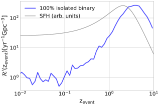
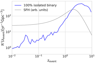
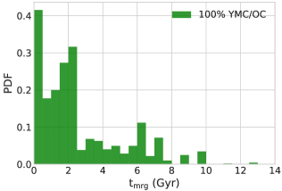
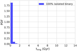
Figure 2: The cosmic evolution of BBH intrinsic merger rate density, ${\mathcal{R}}^{\prime}(z_{\rm event})$ (top panels, green or blue line), and the distribution of merger delay times, $t_{\rm mrg}$ (bottom panels), as obtained from Model Universe stellar populations (Sec. II.3). The left-column panels correspond to the case where the entire star formation in the universe occurs in the form of YMCs of $\gtrsim 10^{4}{\rm M}_{\odot}$. The other two columns correspond to the cases where the entire star formation in the universe occurs in the form of IBs with $\alpha_{\rm CE}=1$ (middle column) and $\alpha_{\rm CE}=3$ (right column). For visual comparison, the grey line (top panels) shows the variation of cosmic SFR with redshift ([85]; not to scale along the Y-axis).

To obtain the inherent dependence of Model Universe merger rate density on redshift (the ‘cosmic merger rate density evolution’), ${\mathcal{R}}^{\prime}_{\rm I}(z_{\rm event})$, the merger events from the sample population are binned according to their event redshifts, $z_{\rm event}$ (see above). The event count, $\Delta{\rm N}_{\rm mrg,I}(z_{\rm event})$, over a redshift bin, $\Delta z_{\rm event}(z_{\rm event})$ around $z_{\rm event}$, is then converted into the corresponding merger rate density, ${\mathcal{R}}^{\prime}_{\rm I}(z_{\rm event})$, by using Eqns. 5-8 and replacing $2\Delta t_{\rm obs}$ (Eqn. 5) by $\Delta t_{\rm age}(z_{\rm event})$. Here, $\Delta t_{\rm age}(z_{\rm event})$ is the universe-age interval corresponding to the redshift interval $\Delta z_{\rm event}(z_{\rm event})$. Note that ${\mathcal{R}}^{\prime}_{\rm I}(z_{\rm event})$ does not include light travel time (which is relevant only for presently observed events) but still incorporates merger delay time and cosmic star-formation and metallicity evolutions.

Although for $\Delta{\rm N}_{\rm mrg,I}(z_{\rm event})$ and ${\mathcal{R}}^{\prime}_{\rm I}(z_{\rm event})$ star formation only up to redshift $z_{\rm event}$ is relevant, applying Eqns. 5-8 is still valid since, for a sufficiently large ${\rm N}_{\rm samp,I}$,

$$\frac{{\rm M}_{\rm samp,I}(z_{\rm event})}{{\rm M}_{\rm samp,I}}=\frac{\int_{t(z=10)}^{t(z=z_{\rm event})}\Phi_{\rm SFH}(z(t))dt}{\int_{t(z=10)}^{t(z=0)}\Phi_{\rm SFH}(z(t))dt}.$$ (11)

Eqn. 11 assumes that the same (effective) fraction of star formation goes into a specific stellar population type, I, throughout the cosmic history. This assumption will be taken throughout this work. As in Ref. [42], 100 equal-sized bins over $0\leq z_{\rm event}\leq 10$ are used to construct ${\mathcal{R}}^{\prime}(z_{\rm event})$. To avoid processing an excessive volume of data over the large range of $z_{\rm event}$, ${\rm N}_{\rm samp,YMC}=2\times 10^{5}$ and ${\rm N}_{\rm samp,IB}=2\times 2500$ are used for this purpose.

In this work, redshift, comoving distance, and light travel time are interrelated (based on a lookup table [92]) according to the $\Lambda$CDM cosmological framework [93, 94]. The cosmological constants from the latest Planck results ($H_{0}=67.4{\rm~{}km~{}s}^{-1}{\rm~{}Mpc}^{-1}$, $\Omega_{\rm~{}m}=0.315$, and flat Universe for which $t_{\rm Hubble}=13.79{\rm~{}Gyr}$ [95]) are applied. Unless otherwise stated (see Sec. III.2), the ‘moderate-Z’ [91] version of the cosmic metallicity evolution is used.

Table 1: Present-day, intrinsic, merger rate density and merger efficiency of BBHs, as obtained from the Model Universe, corresponding to the hypothetical cases where $100\%$ of the star formation takes place in the form of YMCs of $\gtrsim 10^{4}{\rm M}_{\odot}$ or isolated (i.e., never interacting dynamically with each other) field binaries. The values in the second and third sections of this table are for ‘low-Z’ (first row), ‘moderate-Z’ (second row), and ‘high-Z’ (third row) cosmic metallicity evolutions [91] (Sec. III.2).

Channel	Merger rate density $[{\rm~{}yr}^{-1}{\rm Gpc}^{-3}]$	Merger efficiency $[{\rm M}_{\odot}^{-1}]$
100% YMC/OC	${\mathcal{R}}_{\rm YMC}=1635.5$	$\eta_{\rm YMC}=4.30\times 10^{-5}$
100% IB ($\alpha_{\rm CE}=1$)	${\mathcal{R}}_{\rm IB}=13.1$	$\eta_{\rm IB}=1.36\times 10^{-6}$
100% IB ($\alpha_{\rm CE}=3$)	${\mathcal{R}}_{\rm IB}=28.2$	$\eta_{\rm IB}=3.19\times 10^{-6}$
		$\eta_{\rm YMC}=4.49\times 10^{-5}$
100% YMC/OC	$\langle{\mathcal{R}}_{\rm YMC}\rangle=1618.1$	$\eta_{\rm YMC}=4.30\times 10^{-5}$
		$\eta_{\rm YMC}=4.23\times 10^{-5}$
		$\eta_{\rm IB}=3.83\times 10^{-6}$
100% IB ($\alpha_{\rm CE}=3$)	$\langle{\mathcal{R}}_{\rm IB}\rangle=31.6$	$\eta_{\rm IB}=3.17\times 10^{-6}$
		$\eta_{\rm IB}=2.71\times 10^{-6}$

Fig. 1 shows the present-day differential merger rate densities with respect to merger primary mass, ${\rm M}_{1}$ (left panels), and merger mass ratio, $q$ (right panels), for the hypothetical Model Universes with 100% YMC/OC (top row) and 100% IB of $\alpha_{\rm CE}=1$ (middle row) and $\alpha_{\rm CE}=3$ (bottom row). In a universe where all of the star formation converts into pc-scale, gas-free YMCs of $\gtrsim 10^{4}{\rm M}_{\odot}$, $d{\mathcal{R}}_{\rm YMC}/d{\rm M}_{1}$ and $d{\mathcal{R}}_{\rm YMC}/dq$ would greatly exceed than those estimated from GWTC-2 [5], as Fig. 1 suggests. On the other hand, the IB counterpart of this universe would produce GWTC-2-like merger rates but the corresponding $d{\mathcal{R}}_{\rm IB}/d{\rm M}_{1}$ would sharply fall below the GWTC-2 differential rates for ${\rm M}_{1}\gtrsim 20{\rm M}_{\odot}$. The resulting total BBH merger rates corresponding to the two universes are quoted in Table 1. Table 1 also quotes the merger efficiencies, $\eta_{\rm YMC}$ and $\eta_{\rm IB}$, of the two universes. In this work, merger efficiency is simply defined as the number of mergers per unit mass of star formation in a given universe, averaged over redshift and metallicity (i.e., it refers to the universe as a whole rather than a specific type of cluster or a binary population).

Fig. 2 shows the cosmic merger rate density evolutions (left panels) and merger delay time distributions (right panels) for the universes with 100% YMC/OC (top row) and 100% IB of $\alpha_{\rm CE}=1$ (middle row) and $\alpha_{\rm CE}=3$ (bottom row). This figure clearly illustrates the stark difference between the delay times, $t_{\rm mrg}$s, of the BBH mergers originating from YMC/OCs (dynamically-assembled mergers) and IBs (binary-evolutionary mergers). The $t_{\rm mrg}$s from the IBs are mostly concentrated within 500 Myr with a tail in their distribution extending up to 2 Gyr. The predominance of short delay times, in combination with higher formation efficiency of tight BBHs (those with $t_{\rm mrg}<t_{\rm Hubble}$) at lower metallicities [30, 78] that are more dominant at higher $z$, translates into ${\mathcal{R}}^{\prime}_{\rm IB}(z_{\rm event})$ peaking at an epoch earlier than the cosmic-SFH peak. This result has also been found in other recent works that apply similar binary population synthesis approaches (e.g., [78]). The exact form of ${\mathcal{R}}^{\prime}_{\rm IB}(z_{\rm event})$ depends, therefore, on the adopted cosmic metallicity evolution: those in Fig. 2 corresponds to that in Ref. [91] (their ‘moderate-Z’ dependence) as incorporated here. Note that the overall nature of ${\mathcal{R}}^{\prime}_{\rm IB}(z_{\rm event})$ for $\alpha_{\rm CE}=1$ and 3, as obtained here, are similar to those obtained by other recent, similar binary population synthesis studies (e.g., [78, 40]). In contrast, the majority of the $t_{\rm mrg}$s from the YMC/OCs are of $\lesssim 2$ Gyr with a tail in their distribution reaching up to $t_{\rm Hubble}$. The longer $t_{\rm mrg}$s result in ${\mathcal{R}}^{\prime}_{\rm YMC}(z_{\rm event})$ maximizing at a more recent epoch, matching with the SFH peak (see Ref. [42] for further discussions).

III Merger rate density of stellar-mass binary black holes from young massive clusters, open clusters, and isolated binaries

2-channel

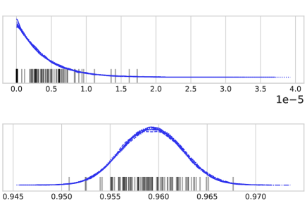
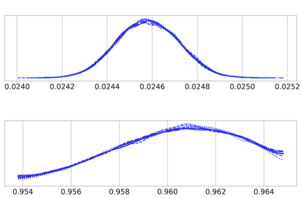
Figure 3: Examples of posterior distributions of $f_{\rm YMC}$ (top panels) and $f_{\rm Obin}$ (bottom panels) in the first and second iterations (left and right panels, respectively) of the Bayesian regression analysis described in Sec. III. This demonstration corresponds to the use of the third moments of $d\mathcal{R}/d{\rm M}_{1}$ and $d\mathcal{R}/dq$ and IB evolution with $\alpha_{\rm CE}=3$. In all panels, the posterior distributions from the 8 MCMC chains (Sec. III) are plotted separately, demonstrating good convergence.

1-channel

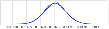
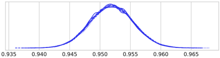
Figure 4: Left: posterior distribution of YMC formation efficiency, $f_{\rm YMC}$, in the Model Universe assuming that the observed, present-day BBH merger rate density [5] is due to the only channel of dynamical interactions inside YMCs/OCs of the universe. Right: posterior distribution of binary fraction among OB stars, $f_{\rm Obin}$, in the Model Universe assuming that the observed, present-day BBH merger rate density is due to the only channel of isolated evolution of massive binaries of the universe. In both panels, the posterior distributions from the 8 MCMC chains (Sec. III) are plotted separately, demonstrating good convergence. These posterior distributions correspond to uninformed priors of $f_{\rm YMC}$ and $f_{\rm Obin}$.

Table 2: The mean value of the posteriors of YMC formation efficiency, $\langle f_{\rm YMC}\rangle$, and that of the OB-star binary fraction, $\langle f_{\rm Obin}\rangle$, for the Model Universe in the various cases indicated in the left column. The posteriors of $f_{\rm YMC}$ and $f_{\rm Obin}$ are obtained from their uninformed priors by applying a two-stage Bayesian regression method as described in Sec. III. $\alpha_{\rm CE}$ is the CE efficiency parameter applied in the isolated-binary (IB) evolution and $p$ is the order of the moment of the present-day differential merger rate density used in the Bayesian analysis. The values in the final section of this table correspond to considering the ‘low-Z’, ‘moderate-Z’, and ‘high-Z’ cosmic metallicity evolutions [91] together (with equal weights).

Channel	$\langle f_{\rm YMC}\rangle$	$\langle f_{\rm Obin}\rangle$
YMC/OC ($p=0$)	$1.69\times 10^{-2}$	$0.0$
IB ($\alpha_{\rm CE}=1,p=0$)	$0.0$	$1.00$
IB ($\alpha_{\rm CE}=3,p=0$)	$0.0$	$9.52\times 10^{-1}$
YMC/OC + IB ($\alpha_{\rm CE}=1,p=0$)	$7.21\times 10^{-3}$	$1.00$
YMC/OC + IB ($\alpha_{\rm CE}=1,p=1$)	$1.04\times 10^{-2}$	$1.00$
YMC/OC + IB ($\alpha_{\rm CE}=1,p=2$)	$1.63\times 10^{-2}$	$1.00$
YMC/OC + IB ($\alpha_{\rm CE}=1,p=3$)	$2.47\times 10^{-2}$	$1.00$
YMC/OC + IB ($\alpha_{\rm CE}=1,p=4$)	$3.74\times 10^{-2}$	$1.00$
YMC/OC + IB ($\alpha_{\rm CE}=3,p=0$)	$1.51\times 10^{-5}$	$9.42\times 10^{-1}$
YMC/OC + IB ($\alpha_{\rm CE}=3,p=1$)	$6.34\times 10^{-3}$	$9.44\times 10^{-1}$
YMC/OC + IB ($\alpha_{\rm CE}=3,p=2$)	$1.50\times 10^{-2}$	$9.12\times 10^{-1}$
YMC/OC + IB ($\alpha_{\rm CE}=3,p=3$)	$2.46\times 10^{-2}$	$9.60\times 10^{-1}$
YMC/OC + IB ($\alpha_{\rm CE}=3,p=4$)	$3.66\times 10^{-2}$	$9.62\times 10^{-1}$
YMC/OC + IB ($\alpha_{\rm CE}=3,p=3$)	$1.48\times 10^{-2}$	$8.69\times 10^{-1}$
YMC/OC + IB ($\alpha_{\rm CE}=3,p=4$)	$2.23\times 10^{-2}$	$9.06\times 10^{-1}$

Having obtained, as in Sec. II.3, the present-day BBH merger rate densities and their cosmic evolutions for the hypothetical YMC-only and IB-only universes, they can be scaled and combined with respect to astrophysical quantities to obtain the merger rate (evolution) in a more realistic universe. The differential and total rates from YMC/OCs are proportional to the YMC formation (as fully-assembled, gas-free YMCs) efficiency, $f_{\rm YMC}$ (the YMC-only universe corresponds to $f_{\rm YMC}=1$). The rates from IBs are proportional to OB-star binary fraction $f_{\rm Obin}$ (the IB-only universe corresponds to $f_{\rm Obin}=1$). If both formation channels contribute to the universe’s BBH mergers, then combined rates are given by

$$\frac{d\mathcal{R}}{dX}(X)=f_{\rm YMC}\frac{d{\mathcal{R}}_{\rm YMC}}{dX}(X)+f_{\rm Obin}\frac{d{\mathcal{R}}_{\rm IB}}{dX}(X)$$ (12)

and

$${\mathcal{R}}^{\prime}(z_{\rm event})=f_{\rm YMC}{\mathcal{R}}^{\prime}_{\rm YMC}(z_{\rm event})+f_{\rm Obin}{\mathcal{R}}^{\prime}_{\rm IB}(z_{\rm event}).$$ (13)

This simple linear combination, of course, assumes that $f_{\rm YMC}$ and $f_{\rm Obin}$ can be represented with constant effective values throughout the cosmic history.

In this study, $f_{\rm YMC}$ and $f_{\rm Obin}$ are determined through a Bayesian-regression approach. The results in Sec. II.3 (see Figs. 1 and 2) suggest that it is important to incorporate the detailed form of the differential rate distributions in determining the relative contributions of various merger channels. Therefore, the likelihood functions are constructed based on various moments of the differential rate density functions from the Model Universe and GWTC-2. The $p$-th moment of the differential merger rate density function defined over an interval $X\in[X1,X2]$ is

$$\mu_{\rm I}^{p}\equiv\int_{X1}^{X2}X^{p}\frac{d{\mathcal{R}}_{\rm I}}{dX}(X)dX.$$ (14)

Therefore, the moment of the combined distribution is (using Eqn. 12)

$$\mu^{p}=\int_{X1}^{X2}X^{p}\frac{d\mathcal{R}}{dX}(X)dX=f_{\rm YMC}\mu_{\rm YMC}^{p}+f_{\rm Obin}\mu_{\rm IB}^{p}.$$ (15)

In the present Bayesian approach, $f_{\rm YMC}\in[0,1]$ and $f_{\rm Obin}\in[0,1]$ are taken to be free parameters to be estimated based on merger rate densities from GWTC-2 and the Model Universe. The elements of the likelihood function are taken to be of the normal form and the priors of $f_{\rm YMC}$ and $f_{\rm Obin}$ are taken to be unbiased. Hence, Bayes theorem [96] becomes

$$P(f_{\rm YMC},f_{\rm Obin}|{\bm{\mu}}_{\rm obs}^{\bm{p}})=$$ (16)

$$\frac{{\mathcal{L}}(f_{\rm YMC},f_{\rm Obin})P(f_{\rm YMC})P(f_{\rm Obin})}{\int\limits_{f_{\rm YMC}}\int\limits_{f_{\rm Obin}}{\mathcal{L}}(f_{\rm YMC},f_{\rm Obin})P(f_{\rm YMC})P(f_{\rm Obin})df_{\rm YMC}df_{\rm Obin}}.$$

Here, $P(f_{\rm YMC},f_{\rm Obin}|{\bm{\mu}}_{\rm obs}^{\bm{p}})$ is the (joint) posterior probability distribution of $f_{\rm YMC}$ and $f_{\rm Obin}$. $P(f_{\rm YMC})$ and $P(f_{\rm Obin})$ are the prior probability distributions of $f_{\rm YMC}$ and $f_{\rm Obin}$, both of which are taken to be uniform over $[0,1]$, ${\mathcal{U}}(0,1)$, at the initial iteration (see below). ${\mathcal{L}}(f_{\rm YMC},f_{\rm Obin})$ is the likelihood function given by

$${\mathcal{L}}(f_{\rm YMC},f_{\rm Obin})=P({\bm{\mu}}_{\rm obs}^{\bm{p}}|f_{\rm YMC},f_{\rm Obin})$$ (17)

$$=\prod_{i}^{N_{\rm obs}}{\mathcal{N}}\left[\mu^{p}(f_{\rm YMC},f_{\rm Obin})-\mu_{\rm obs,i}^{p},\Delta\mu^{p}(f_{\rm YMC},f_{\rm Obin})\right].$$

Here, ${\mathcal{N}}[\mu,\sigma]$ represents a normal probability distribution with mean $\mu$ and variance $\sigma^{2}$. $\mu_{\rm obs,i}^{p}\in{\bm{\mu}}_{\rm obs}^{\bm{p}}$ are the moments of the GWTC-2 intrinsic differential merger rate densities. To obtain these, $N_{\rm obs}=300$ random values of the posteriors of GWTC-2 differential merger rate densities (their ‘power law + peak’ model) are chosen at each bin (the orange dots in the panels of Fig. 1). The resulting $N_{\rm obs}$ different distributions then give $N_{\rm obs}$ different values, $\mu_{\rm obs,i}^{p}$. $\mu^{p}(f_{\rm YMC},f_{\rm Obin})$ is the combined Model Universe moment as given by Eqn. 15. $\Delta\mu^{p}(f_{\rm YMC},f_{\rm Obin})$ is a measure of the variance of the Model Universe moment given by (follows from Eqn. 15)

$$\Delta\mu^{p}=f_{\rm YMC}\Delta\mu_{\rm YMC}^{p}+f_{\rm Obin}\Delta\mu_{\rm IB}^{p}.$$ (18)

(For brevity, $\mu^{p}(f_{\rm YMC},f_{\rm Obin})$ and $\Delta\mu^{p}(f_{\rm YMC},f_{\rm Obin})$ will hereafter be written without the arguments.) $\Delta\mu_{\rm I}^{p}$ comprises errors from all the bins, i.e.(following from Eqn. 14; taking idealized parameter estimation in the Model Universe implying $\Delta X=0$),

$$\Delta\mu_{\rm I}^{p}=\int_{X1}^{X2}X^{p}\left[\Delta\frac{d{\mathcal{R}}_{\rm I}}{dX}(X)\right]dX.$$ (19)

In practice, $\Delta(d{\mathcal{R}}_{\rm I}/dX)$ at a particular bin is determined by stacking the outcomes of the independent sample-population trials and taking the difference of the resulting maximum and minimum rates, for that bin (Eqns. 9-10). For single SFH, age-redshift, and metallicity-redshift dependencies, as used in the Model Universe (Sec. II.3), $\Delta(d{\mathcal{R}}_{\rm I}/dX)$ is comparable to that due to the Poisson error in the bin. However, larger variations would result by incorporating astrophysical variations, as demonstrated below (Sec. III.2).

To take into account the present-day differential merger rate density distributions with respect to both $q$ and ${\rm M}_{1}$, a two-step procedure is followed. First, the posteriors of $f_{\rm YMC}$ and $f_{\rm Obin}$ are obtained (Eqn. 15-19), assuming their ${\mathcal{U}}(0,1)$ prior distributions, by considering the moments of only the rate distributions with respect to $q$. The resulting posteriors of $f_{\rm Obin}$ are then treated as priors of the same in the next iteration. In this following iteration, the posteriors of $f_{\rm YMC}$ and $f_{\rm Obin}$ are redetermined by considering the moments of only the rate distributions with respect to ${\rm M}_{1}$ and resetting the prior distribution of $f_{\rm YMC}$ to ${\mathcal{U}}(0,1)$. The resulting posteriors are taken to be final.

The construction of the likelihood function and the sampling of the posteriors are done utilizing the Python package ${\tt PyMC3}$ [97], using its Uniform, Normal, Interpolated, and sample utilities. The posteriors are obtained by applying a (Hamiltonian) Markov Chain Monte Carlo (hereafter MCMC) approach that employs the No U-turn Sampler of the package. $8\times 12500$ posterior samples (plus $8\times 1500$ tuning iterations) are drawn from 8 independent MCMC chains. For each chain, the first 1000 values are discarded (or ‘burned’) to avoid incorporating spurious values in the posterior distributions.

This two-stage procedure is inspired by the fact that despite the large difference in amplitude, $d{\mathcal{R}}_{\rm YMC}/dq$ and $d{\mathcal{R}}_{\rm IB}/dq$ are of similar shape and truncations unlike $d{\mathcal{R}}_{\rm YMC}/d{\rm M}_{1}$ and $d{\mathcal{R}}_{\rm IB}/{\rm M}_{1}$ which are largely dissimilar (Sec. II.3; Fig. 1). Hence, one can first ‘learn’ about $f_{\rm Obin}$ from the $q$ distributions and then further refine the inferences on $f_{\rm YMC}$ and $f_{\rm Obin}$ from the ${\rm M}_{1}$ distributions. That way, zero to a few divergences among the MCMC chains (as reported by the sampler summary) are always obtained at the end of the second sampling iteration. The posterior distributions of $f_{\rm YMC}$ and $f_{\rm Obin}$ from the two iterations are shown in the example of Fig. 3, which shows excellent agreement between the final distributions obtained from the 8 MCMC chains separately. Such MCMC traces are plotted using the ArviZ package [97]. The rest of the figures in this paper are plotted using Matplotlib[98] .

A simpler, single-iteration version of the above procedure is applied for a one-channel universe, i.e., where BBH mergers are produced from either YMC/OC or field binaries having fractions $f_{\rm YMC}$ or $f_{\rm Obin}$, respectively. In other words, Eqns. 15 and 18 have $f_{\rm Obin}=0$ or $f_{\rm YMC}=0$, respectively. In this case, only the zeroth moment (i.e., total rate) of the $q$ distributions are utilized for a one-stage estimation of $f_{\rm YMC}$ ($f_{\rm Obin}$) posteriors, taking the prior distribution of $f_{\rm YMC}$ ($f_{\rm Obin}$) to be ${\mathcal{U}}(0,1)$. This exercise, typically, also yields good convergence. Fig. 4 shows such an example of posteriors from the 8 MCMC sampling chains.

Note that the present method is still preliminary and proof-of-concept. In particular, no ‘hyper-parameter’ is applied. Such parameters can be, e.g., SFH slope, metallicity-redshift slope, cluster-structural parameters, binary-physics parameters, BH-spins, that determine the probabilities of present-day merger and detection beyond a signal-to-noise-ratio threshold. In a future work, such a more complete Bayesian analysis and inference [99, 100] will be explored. The present exercise, although explicitly involves Bayes theorem and data from theoretical models and from analyses of observed event parameters (specifically, GWTC-2 ‘power law + peak’ intrinsic merger rate densities), can be described as a ‘Bayesian regression’ procedure.

III.1 One-channel universe

Fig. 5 (top panels) shows the $d\mathcal{R}/d{\rm M}_{1}$ and $d\mathcal{R}/dq$ for the Model Universe with $f_{\rm Obin}=0$, i.e., when only YMC/OCs of the universe produce BBH mergers. The Model Universe rates are plotted for 200 random choices of the posteriors of $f_{\rm YMC}$. The mean of the $f_{\rm YMC}$ posteriors is stated in Table 2. The corresponding ${\mathcal{R}}^{\prime}(z_{\rm event})$ (up to $z_{\rm event}=1$) is shown in the bottom panel of Fig. 5. See the figure’s caption for further detail. Fig. 5 essentially reproduces the results obtained in Ref. [42] but with differently-obtained normalization. It suggests that, in principle, dynamical BBH mergers in moderate-mass YMCs and OCs in the Universe alone can self-consistently explain the present-day, differential intrinsic BBH merger rate density and the cosmic evolution of intrinsic BBH merger density, as inferred from GWTC-2. However, for $z_{\rm event}\lesssim 0.2$, ${\mathcal{R}}^{\prime}$ falls below the GWTC-2 median by a few factors and reaches the GWTC-2 lower limit at $z_{\rm event}\approx 0$ (Fig. 5, lower panel). Of course, the very high ${\mathcal{R}}_{\rm YMC}$ of the 100%-YMC universe (Sec. II.3, Table 1) results in the inference of the small mean $\langle f_{\rm YMC}\rangle\sim 10^{-2}$ (Table 2).

The two sets of panels in Fig. 6 analogously show the outcomes of the Model Universe with $f_{\rm YMC}=0$, i.e., when only IBs of the universe produce BBH mergers. The upper (lower) set is for IBs with $\alpha_{\rm CE}=1$ ($\alpha_{\rm CE}=3$). Fig. 6 suggests that with mean $\langle f_{\rm Obin}\rangle\approx 1.0$ (see Table 2) for $\alpha_{\rm CE}=1$ and $\alpha_{\rm CE}=3$, the Model Universe $d\mathcal{R}/d{\rm M}_{1}$ falls short of the GWTC-2 rates for ${\rm M}_{1}\gtrsim 20{\rm M}_{\odot}$. The Model Universe $d\mathcal{R}/dq$, however, well reproduces the corresponding GWTC-2 differential rates down to $q\approx 0.4$, especially with $\alpha_{\rm CE}=3$. The corresponding ${\mathcal{R}}^{\prime}(z_{\rm event})$ falls below the GWTC-2 lower limit for $z_{\rm event}\lesssim 0.4$, for both $\alpha_{\rm CE}$.

A binary fraction of $f_{\rm Obin}\gtrsim 90$% is consistent with the observed high binary fraction among OB-stars in clusters and in the Galactic field [51, 52, 53]. YMC formation efficiency is a much more ambiguous and poorly determined quantity [101, 102, 56]. The inferred $f_{\rm YMC}\sim 10^{-2}$ is consistent with the results from recent cosmological-hydrodynamical simulations of galaxy and cluster formation [103], for upper cutoff of $>10^{5}{\rm M}_{\odot}$ of the young cluster mass distribution as applicable for the present YMC models.

1-channel: YMC/OC

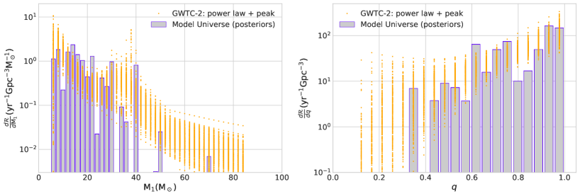
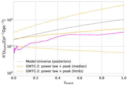
Figure 5: The Model Universe present-day, differential intrinsic merger rate density of BBHs (top panels; the legends are the same as in Fig. 1) and the cosmic evolution of BBH intrinsic merger rate density (bottom panel, magenta line), assuming that the observed, present-day BBH merger rate density [5] is due to the only channel of dynamical interactions inside YMCs/OCs of the universe. The Model Universe rates shown in these panels correspond to 200 choices of the posteriors of $f_{\rm YMC}$ in the YMC-only universe, as shown in Fig. 4. The orange solid (dashed) line(s) in the bottom panel depict the median (90%-credible limits) of the GWTC-2 cosmic merger rate density evolution: these lines are given by ${\mathcal{R}}^{\prime}(z_{\rm event})=19.3_{-9.0}^{+15.1}{\rm~{}yr}^{-1}{\rm Gpc}^{-3}(1+z_{\rm event})^{1.3_{-2.1}^{+2.1}}$ [5, their power law + peak model]. As in Fig. 2, the grey line (bottom panel) depicts the variation of cosmic SFR with redshift (arbitrary unit along the Y-axis).

1-channel: IB ($\alpha_{\rm CE}=1$)

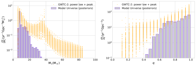
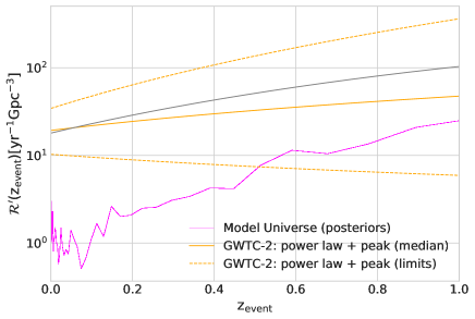
1-channel: IB ($\alpha_{\rm CE}=3$)

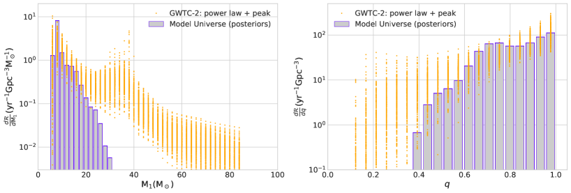
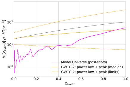
Figure 6: The same description as in Fig. 5 applies to both of the 3-panel sets except for the assumption here that the Model Universe produces BBH mergers only due to isolated evolution of massive binaries. Accordingly, the posteriors of $f_{\rm Obin}$ in the IB-only universe (Fig. 4) are applied. The cases for $\alpha_{\rm CE}=1$ (top set) and $\alpha_{\rm CE}=3$ (bottom set) are shown.

III.2 Two-channel universe

Fig. 7 shows the combined $d\mathcal{R}/d{\rm M}_{1}$ and $d\mathcal{R}/dq$ for the two-channel Model Universe where BBH mergers are produced both dynamically in YMC/OCs and through IB evolution (Sec. III). The Model Universe differential rates are shown for the Bayesian regression analyses using moments of order $p=1$, 2, 3, and 4 of the rate distributions (Sec. III) and taking $\alpha_{\rm CE}=1$ for the IB evolution. Fig. 8 shows the corresponding combined ${\mathcal{R}}^{\prime}(z_{\rm event})$ evolutions (up to both $z_{\rm event}=10$ in logarithmic scale and $z_{\rm event}=1$ in linear scale). Fig. 9 and 10 show the Model Universe combined $d\mathcal{R}/d{\rm M}_{1}$, $d\mathcal{R}/dq$, ${\mathcal{R}}^{\prime}(z_{\rm event})$ yields when the IBs in the Model Universe evolve with $\alpha_{\rm CE}=3$; the results with $p=3$ and 4 are shown.

With moments of increasing order included in the analysis, $\langle f_{\rm YMC}\rangle$ increases whereas $\langle f_{\rm Obin}\rangle$ stays nearly constant at $\approx 1.0$ ($\approx 0.9$) for $\alpha_{\rm CE}=1$ ($\alpha_{\rm CE}=3$); see Table. 2. This results in overall increase of the present-day, combined differential rates and of the combined total rate at lower redshifts ($z_{\rm event}\lesssim 1$). The high redshift behaviour of ${\mathcal{R}}^{\prime}$ is still dominated by the contribution from IBs (for both $\alpha_{\rm CE}$) so that the combined ${\mathcal{R}}^{\prime}$ is peaked much earlier (at $z_{\rm event}\approx 4$) than the cosmic SFH, similarly as ${\mathcal{R}}^{\prime}_{\rm IB}$. With $\langle f_{\rm Obin}\rangle\gtrsim 0.9$ and $\langle f_{\rm YMC}\rangle\lesssim 10^{-2}$, ${\mathcal{R}}^{\prime}$ would be dominated by ${\mathcal{R}}^{\prime}_{\rm IB}$ at high redshifts as Fig. 2 suggests (see also discussions in Sec. II.3).

The increase of $\langle f_{\rm YMC}\rangle$ with moment-order, $p$, is due to the fact that higher order moment would amplify the dependence on larger ${\rm M}_{1}$, where YMC/OCs contribute to the GWTC-2 rates essentially solely. As seen in Fig. 1, for both $\alpha_{\rm CE}$, the profile of $d{\mathcal{R}}_{\rm IB}/d{\rm M}_{1}$ declines steeply from ${\rm M}_{1}\gtrsim 20{\rm M}_{\odot}$ and cuts off at ${\rm M}_{1}\approx 30{\rm M}_{\odot}$. As opposed to this, the $d{\mathcal{R}}_{\rm YMC}/d{\rm M}_{1}$ profile continues much more smoothly up to $\approx 50{\rm M}_{\odot}$ and also contains discrete events beyond, in the PSN gap (the PSN-gap BHs being produced via either first-generation BBH mergers or BH-Thorne-Zytkow-Object accretion; see Ref. [48] for details). On the other hand, $d{\mathcal{R}}_{\rm IB}/dq$ already fits well (for both $\alpha_{\rm CE}$; see Fig. 1), without any scaling, the corresponding GWTC-2 rates over $q\gtrsim 0.5$ where most of the total rate is accumulated. Hence, $\langle f_{\rm Obin}\rangle$ is essentially ‘settled’ from the $q$ dependence of the GWTC-2 and IB rates. As discussed in Sec. III, it is these features of the Model Universe differential rates vis-á-vis those from GWTC-2 that motivates the two-stage Bayesian regression applied in the 2-channel case.

With $p=3$ and 4, the two-channel Model Universe $d\mathcal{R}/d{\rm M}_{1}$, $d\mathcal{R}/dq$, and ${\mathcal{R}}^{\prime}(z_{\rm event})$ all agree well with those from GWTC-2 over the relevant ranges of ${\rm M}_{1}$, $q$, and $z_{\rm event}$, as seen in Figs. 7, 8, 9, 10. This is as opposed to the one-channel universe where the agreements are partial (see Sec. III.1) despite similar estimated values of $f_{\rm YMC}$ and $f_{\rm Obin}$ (see Table 2).

All the Model Universe rates, obtained so far, have small variance. This is due to the small, of the order of Poisson error, variance that goes into the likelihood functions, Eqn. 17 (see Sec. III). Introducing astrophysical uncertainties in the ingredients of the Model Universe would increase the uncertainties in its rates, as demonstrated here by altering the redshift-metallicity relation.

The population synthesis exercises of IB-only and YMC-only universes (Sec. II.3) are repeated also with the ‘low-Z’ and ‘high-Z’ cosmic metallicity evolutions [91]. The two-channel universe is then rerun with $\Delta\mu_{\rm I}^{p}$s recalculated similarly (Sec. III) but after stacking outcomes, in equal numbers, from the ‘low-Z’, ‘moderate-Z’, and ‘high-Z’ trials. The $\mu_{\rm I}^{p}$s used in the run are also equal-weighted average of the $d{\mathcal{R}}_{\rm I}/dX$s obtained from the three redshift-metallicity dependencies.

Fig. 11 shows the resulting $d{\mathcal{R}}_{\rm I}/dX$s (100% universes) with the increased error bars. Fig. 12 shows the resulting $d\mathcal{R}/d{\rm M}_{1}$, $d\mathcal{R}/dq$, and ${\mathcal{R}}^{\prime}(z_{\rm event})$ from the two-channel universe (for $p=4$ and $\alpha_{\rm CE}=3$ IB evolution). The corresponding total merger rates, merger efficiencies, $\langle f_{\rm YMC}\rangle$, and $\langle f_{\rm Obin}\rangle$ are quoted in Tables 1 and 2. Overall, Fig. 12 exhibits similarly good agreement with the GWTC-2 rates as in the previous figures with similar estimated values of $\langle f_{\rm YMC}\rangle$ and $\langle f_{\rm Obin}\rangle$. It is, however, important to stress that the error analysis, as presented above, is incomplete and serves only as a demonstration. To incorporate uncertainties in a more complete manner, additional astrophysical sources of uncertainties, e.g., variations of the SFH, alternative cosmic metallicity evolutions, varied binary evolution physics (e.g., $\alpha_{\rm CE}$), wider ranges of cluster structure and initial condition [e.g., 104, 105, 106, 33, 77, 107, 108] needs to be considered. The above exercise demonstrates that the present data-driven approach can naturally include outcomes from population syntheses with any set of model assumptions and thus, in principle, can simultaneously incorporate multiple astrophysical uncertainties.

2-channel: YMC/OC + IB ($\alpha_{\rm CE}=1$)

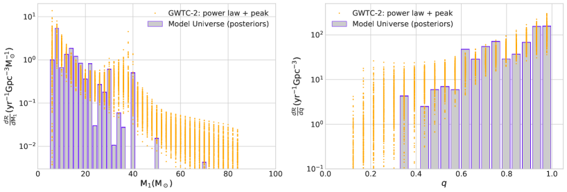
Figure 7: The filled histogram is the present-day, differential intrinsic merger rate density of BBHs of the Model Universe as obtained by combining those due to the YMC/OC and IB channels using the posteriors of $f_{\rm YMC}$ and $f_{\rm Obin}$. The Model Universe posteriors are obtained by the two-step Bayesian regression approach described in Sec. III (see Fig. 3 for an example). Row 1, 2, 3, and 4 corresponds to the use of the first, second, third, and fourth moments of $d\mathcal{R}/d{\rm M}_{1}$ and $d\mathcal{R}/dq$ (IB evolution with $\alpha_{\rm CE}=1$), respectively. On each panel, combined differential merger rate densities for 200 pairs of random and independent draws from the posteriors of $f_{\rm YMC}$ and $f_{\rm Obin}$ are superposed. As before, the orange dots are random draws (300 per bin) of the posteriors of BBH differential intrinsic merger rate densities obtained by the LVK GWTC-2 (their power law + peak model).

2-channel: YMC/OC + IB ($\alpha_{\rm CE}=1$)

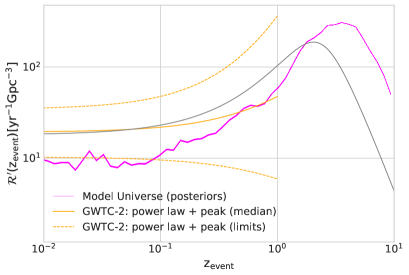
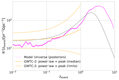
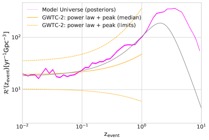
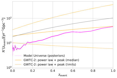
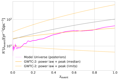
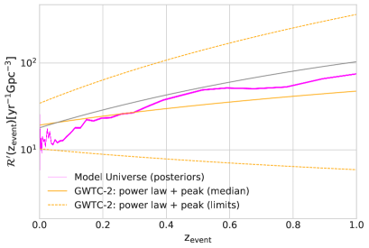
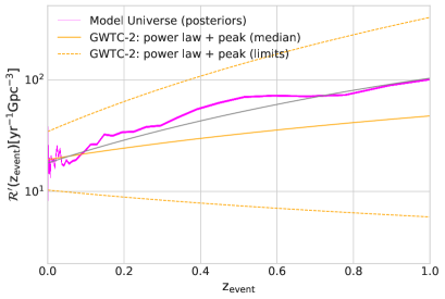
Figure 8: The magenta line (all panels) represents the redshift-evolution of Model Universe BBH merger rate density from the YMC/OC and IB channels combined. As in Fig. 7, the Model Universe posteriors of $f_{\rm YMC}$ and $f_{\rm Obin}$ (200 random and independent pairs of them) are applied to combine the rates from the two channels. The first, second, third, and fourth panel corresponds to the use of the first, second, third, and fourth moments of $d\mathcal{R}/d{\rm M}_{1}$ and $d\mathcal{R}/dq$ (IB evolution with $\alpha_{\rm CE}=1$), respectively. As in Fig. 5, the orange lines depict the corresponding GTWC-2 median and 90% confidence limits (power law + peak model). As before, the grey line depicts the variation of cosmic SFR with redshift (arbitrary unit along the Y-axis). Panels fifth to eighth re-plot these in the same order with the X-axis in linear scale and truncated at redshift $1.0$.

2-channel: YMC/OC + IB ($\alpha_{\rm CE}=3$)

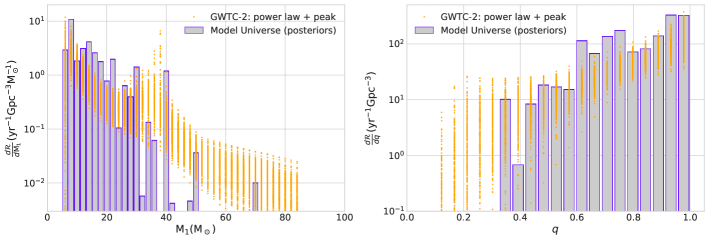
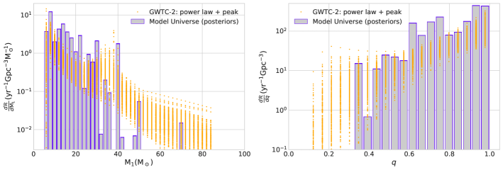
Figure 9: The same description of Fig. 7 applies here except that the IB-evolution is with $\alpha_{\rm CE}=3$. The top (bottom) panel corresponds to utilizing the third (fourth) moment of the differential rates.

2-channel: YMC/OC + IB ($\alpha_{\rm CE}=3$)

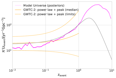
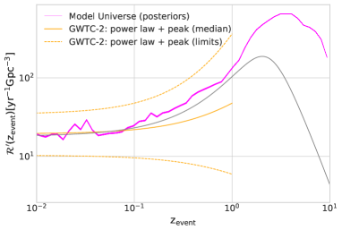
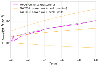
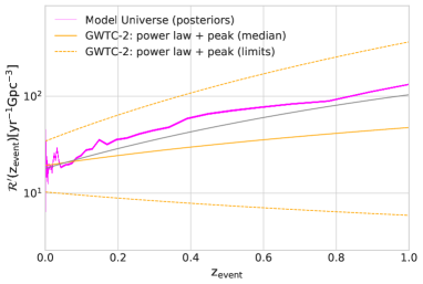
Figure 10: The same description of Fig. 8 applies here except that the IB-evolution is with $\alpha_{\rm CE}=3$. The upper-left (-right) panel corresponds to utilizing the third (fourth) moment of the differential rates. The lower panels re-plot these in the same order with the X-axis in linear scale and truncated at redshift $1.0$.

Pure channel: YMC/OC and IB ($\alpha_{\rm CE}=3$)

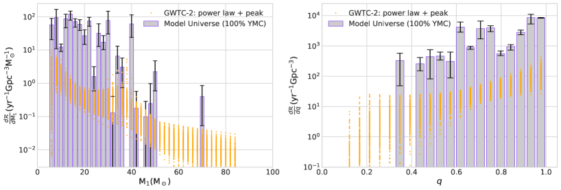
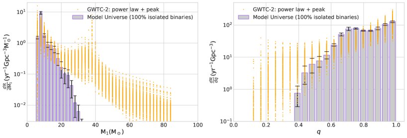
Figure 11: The same description as for Fig. 1 applies. For the IB channel (lower panels), only the $\alpha_{\rm CE}=3$ case is shown. The error bars are due to the three different variants of cosmic metallicity evolution history in Ref. [91], namely, their ‘low-Z’, ‘moderate-Z’, and ‘high-Z’ evolutions (equal weights applied).

2-channel: YMC/OC + IB ($\alpha_{\rm CE}=3$)

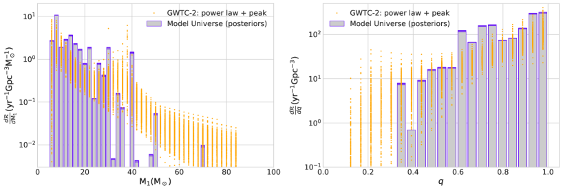
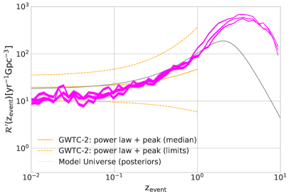
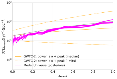
Figure 12: The combined, YMC/OC + IB ($\alpha_{\rm CE}=3$) present-day differential merger rate density of BBHs (top panels) and cosmic BBH merger rate density evolution (bottom panels) as obtained from the Model Universe. To obtain the posteriors of $f_{\rm YMC}$ and $f_{\rm Obin}$, the differential merger rate densities corresponding to the ‘low-Z’, ‘moderate-Z’, and ‘high-Z’ cosmic metallicity evolutions [91] are considered together (with equal weights), as shown in Fig. 11. In this example, fourth moments of the differential rates are applied.

IV Summary and concluding remarks

This study attempts to combine two widely investigated channels of stellar-mass BBH mergers in the Universe, namely, dynamical interactions involving stellar-mass BHs inside YMCs evolving into medium mass OCs (the YMC/OC channel) and evolution of isolated massive binaries in the field (the isolated-binary or IB channel). Cosmological population syntheses are performed with (hypothetical) universes comprising only model YMC/OCs or IBs (Secs. II.1, II.2), taking into account $\Lambda$CDM background cosmology and observation-based cosmic star-formation and metallicity evolutions (Sec. II.3; Figs. 1, 2). The resulting present-day differential intrinsic BBH merger rate density from both universes are then linearly combined assuming constant effective values of YMC formation efficiency, $f_{\rm YMC}$, and OB-star binary fraction, $f_{\rm Obin}$, throughout the cosmic history. The quantities $f_{\rm YMC}$ and $f_{\rm Obin}$ are then estimated, based on present-day differential intrinsic BBH merger rate density from GWTC-2, by applying a two-stage linear Bayesian regression involving moments of the rate distributions (Sec. III).

The resulting Model Universe, combined, present-day differential BBH merger rate density and also the cosmic evolution of the combined, total BBH merger rate density agree well with those from GWTC-2 (Sec. III.2; Figs. 7, 8, 9, 10). The agreements from the two-channel universe are better and more complete than those from the one-channel universes (Sec. III.1; Figs. 5, 6) where BBH mergers are assumed to be produced via either YMC/OC dynamics or IB evolution. The estimated $\langle f_{\rm Obin}\rangle\gtrsim 90$% (see Table 2) is in agreement with the observed high binary fraction among OB stars. The estimated $\langle f_{\rm YMC}\rangle\sim 10^{-2}$ is consistent with cluster formation efficiencies from recent cosmological simulations.

The physical interpretation of $f_{\rm YMC}$ and $f_{\rm Obin}$ should, however, be taken with caution. This is especially so for $f_{\rm YMC}$: cluster formation efficiency is itself subject to varied interpretations (e.g., [109, 102, 55]). From methodological point of view, $f_{\rm YMC}$ and $f_{\rm Obin}$ simply serve like ‘branching ratio’ or ‘mixing fraction’ [39, 100], determining the relative contributions from the two merger channels.

The present results suggest that despite significant BBH-merger contributions from dynamics in YMCs and OCs at low redshifts, high-redshift ($z_{\rm event}\gtrsim 1$) behaviour of the BBH merger rate density is still determined by the physics of binary evolution (Sec. III.2). Hence, future GW detectors with increased visibility horizons, e.g., LVK A+ and A++ upgrades, Voyager, Einstein Telescope, Cosmic Explorer will potentially be able to provide information regarding the physical processes in massive-star binaries that drive compact binary mergers from them. Similar conclusion is drawn in recent independent studies involving similar binary population synthesis in a one-channel universe (e.g., [78, 40]).

Note that all the estimates and hence the conclusions in this study are subject to the specifics of the YMC/OC- and IB-evolutionary models (Secs. II.1,II.2). Especially, BBH (and other compact-binary) mergers from IB evolution is sensitive to crucial binary-evolution ingredients such as models of tidal interaction, mass transfer, and CE evolution [30, 47, 76]. The direct N-body evolutionary models of YMC/OCs treat all Newtonian and PN interactions explicitly, member-by-member, and without any symmetry assumptions or modelling them [62]. Also, the vast majority of the YMC/OC BBH mergers are dynamically assembled inside the clusters and hence they do not depend explicitly on binary-evolution physics. However, the same ${\tt BSE}$ that is used for IB evolutions also goes into the stellar- and binary-evolution modelling during the N-body integration, shaping the mass distribution of the BHs retained in the cluster (which BHs, eventually, participate in dynamical pairings). The BH mass distribution depends on ${\tt BSE}$’s modelling of star-star and star-BH mergers and also the ingredients of binary evolution modelling (tidal interaction, mass transfer, CE evolution) that drive these events [110, 47, 48].

The present study is a proof-of-concept demonstration utilizing computations of model YMC/OCs and IBs. It demonstrates a simplistic linear Bayesian regression chain involving only raw moments, which statistics are biased quantities. This will be improved in a future work by incorporating central moments and/or moments around multiple axes. While all the analyses and comparisons in this work are done based on an underlying or intrinsic population model of the LVK (their power law + peak model), it is important and more model-independent to compare directly with the posterior samples of the event parameters from GWTC-2 (and future GW-event catalogues) [99, 111, 100]. The analysis will also benefit by refining the metallicity coverage and expanding the range of $\alpha_{\rm CE}$ of the IB-evolutionary models [e.g., 112, 113].

In the present demonstration, only two BBH merger channels are considered. Additional merger channels and additional types of compact-binary mergers (i.e., NS-BH and BNS mergers) can be incorporated via straightforward extensions. Other widely explored channels to consider are chemically-homogeneous binary evolution, many-body dynamics in GCs, low mass young clusters, and nuclear clusters, few-body dynamics in field hierarchical systems and AGN gas discs, pairing of BHs derived from Population-III stars [e.g., 114, 18, 115, 116, 117, 118, 22, 38, 119, 120]. Such range of channels would also help filling up the more extreme regions of the differential rate distributions (e.g., those with ${\rm M}_{1}$ in the PSN gap and $q\lesssim 0.3$).