Lorentz symmetry in ghost-free massive gravity

Abstract

The role of Lorentz symmetry in ghost-free massive gravity is studied, emphasizing features emerging in approximately Minkowski spacetime. The static extrema and saddle points of the potential are determined and their Lorentz properties identified. Solutions preserving Lorentz invariance and ones breaking four of the six Lorentz generators are constructed. Locally, globally, and absolutely stable Lorentz-invariant extrema are found to exist for certain parameter ranges of the potential. Gravitational waves in the linearized theory are investigated. Deviations of the fiducial metric from the Minkowski metric are shown to lead to pentarefringence of the five wave polarizations, which can include superluminal modes and subluminal modes with negative energies in certain observer frames. The Newton limit of ghost-free massive gravity is explored. The propagator is constructed and used to obtain the gravitational potential energy between two point masses. The result extends the Fierz-Pauli limit to include corrections generically breaking both rotation and boost invariance.

I Introduction

The foundational symmetries of General Relativity (GR) include local Lorentz invariance and diffeomorphism invariance, which exclude the graviton from acquiring a mass. In linearized gravity, a massive graviton propagating on Minkowski spacetime can be described by the Fierz-Pauli term fp39 . However, in the limit of vanishing mass, the Fierz-Pauli term is discontinous to linearized GR vvd70 ; vz70 , as in addition to the usual graviton modes it yields a massless scalar mode, the Boulware-Deser ghost bd72 . A theory of massive gravity reducing to GR in the massless limit requires instead a nonlinear completion av72 . This can be constructed using a special nonlinear potential that eliminates the ghost mode due to the appearance of an extra second-class constraint drgt11 . The action for massive gravity can be formulated using two metrics, a dynamical metric $g_{\mu\nu}$ and a nondynamical fiducial metric $f_{\mu\nu}$ hr11 , combined in a five-parameter quartic potential that removes the two ghost degrees of freedom hr1112 . The theory of massive gravity and its developments, including bimetric and multimetric versions, are reviewed in Refs. kh11 ; dr14 ; ss16 .

The nondynamical fiducial metric $f_{\mu\nu}$ in ghost-free massive gravity can be viewed as a prescribed background field that explicitly breaks the spacetime symmetries of GR in a special way, thereby permitting a nonzero graviton mass with no ghost mode. Astrophysical constraints require the graviton mass to be less than $10^{-38}$ GeV gn10 , so a nonzero value would represent a phenomenologically tiny deviation from GR. In a broad context, small deviations from a specified theory can be described in a model-independent way using effective field theory sw09 . The general effective field theory containing all terms breaking the spacetime symmetries of GR and its couplings to matter has been developed ak04 . This framework provides conceptual insights about the breaking of spacetime symmetries in various theories modifying GR and remains the subject of ongoing investigation, with numerous experiments performed to measure the coefficients governing the symmetry breaking tables . For ghost-free massive gravity, it enables the derivation of constraints on matter couplings from searches for Lorentz violation bbw19 .

In this work, we investigate some specific implications of the breaking of spacetime symmetries in ghost-free massive gravity. Our focus is primarily on properties related to the Lorentz transformations that emerge in approximately Minkowski spacetime, although we expect many of the concepts to apply in other background spacetimes as well. These Lorentz transformations arise from a combination of local Lorentz and diffeomorphism transformations in curved spacetime kl21 and moreover are the focus of most experimental investigations tables , so they are of particular interest in the present context. Here, we explore two topics along these lines. The first concerns the static extrema and saddle points of the potential and their Lorentz structure. We show the theory admits a variety of solutions including ones that are Lorentz invariant and others that are Lorentz violating, and we classify the patterns of symmetry breaking. We determine the local, global, and absolute stability of the solutions, verifying that an absolutely stable Lorentz-invariant extremum exists for special potential parameters.

The second topic concerns the phenomenology of flat non-Minkowski fiducial metrics, $f_{\mu\nu}\not\propto\eta_{\mu\nu}$. In approximately Minkowski spacetime, these can in principle generate observable signals of explicit Lorentz violation. We study two scenarios of potential experimental interest, gravitational waves and the limit of Newton gravity. For gravitational waves representing excitations about Minkowski spacetime, we demonstrate that the five modes of massive gravity experience pentarefringence during propagation. The modes are either superluminal or carry negative energies in some observer frames, a result typical of Lorentz-violating theories kl01 . For Newton gravity, we obtain the propagator and use it to determine the gravitational potential energy between two point masses. The modifications to the usual Yukawa form for the Fierz-Pauli case include violations of both boost and rotation invariance.

The organization of this work is as follows. In Sec. II, we present essential preliminary material. The action for massive gravity adopted here and the definitions of relevant variables are presented in Sec. II.1. A summary of the spacetime symmetries of the theory is provided in Sec. II.2, along with an outline of their implementation in approximately Minkowski spacetime. In Sec. II.3, a decomposition of the key matrix variable convenient for calculational purposes is performed.

The investigation of extrema and saddle points of the action is undertaken in Sec. III. We obtain the potential governing static solutions and solve the resulting equations of motion for flat fiducial metrics. Three cases are distinguished, treated in turn in Secs. III.1, III.2, and III.3. The static solutions are constructed and their Lorentz properties established. In each case, the issue of local stability, instability, or metastability is addressed using the technique of bordered hessians. The surface generated by the hamiltonian constraint and the positions of the solutions on its connected sheets are used to establish global and absolute stability properties.

In Sec. IV, the linearized limit of massive gravity is explored. We investigate the Lorentz properties of solutions of the modified linearized Einstein equation that reduce to Minkowski spacetime for vanishing fluctuations of the dynamical metric. Gravitational waves are considered in Sec. IV.1. We construct the eigenenergies and eigenmodes of the modified Einstein equation and study their splitting for choices of the fiducial metric that differ from the Minkowski metric. The limit of Newton gravity is examined in Sec. IV.2. The propagator for linearized massive gravity is obtained and used to determine the gravitational potential energy between two stationary point masses. An overall summary of the paper is provided in Sec. V, while Appendix A describes technical details of certain integrals required in the text. The conventions for metric, curvature, and other signs and factors are those of Ref. ak04 , Appendix A.

II Setup

In this section, we discuss the form of the action for massive gravity used in the present work. We summarize key aspects of spacetime symmetries and their violations, and we provide a matrix decomposition for the dynamical variable of central interest in the analyses to follow.

II.1 Basics

Consider the action for ghost-free massive gravity in the form hr11

$$S=\frac{1}{2\kappa}\int d^{4}x\sqrt{-g}\Big{(}R-2m^{2}\sum_{n=0}^{4}\beta_{n}e_{n}(\mathbb{X})\Big{)}+S_{\rm m},$$ (1)

where $\kappa=8\pi G$. The first term is the usual Einstein-Hilbert action written in terms of the dynamical metric $g_{\mu\nu}$ and the Riemann scalar curvature $R$. The second term can be understood as a nonderivative scalar potential for the dynamical metric, which depends on the mass scale $m$ and on five dimensionless parameters $\beta_{n}$, $n=0,\ldots,4$. Only two combinations of the latter have independent physical meaning hr11 . To ensure that the matrix of Poisson brackets of second class constraints is invertible, the parameters satisfy the condition sa14 $\beta_{1}+2\beta_{2}+\beta_{3}\neq 0$.

The potential in the action (1) also involves a nondynamical fiducial metric $f_{\mu\nu}$, which can be chosen as desired but is often taken to be the Minkowski metric $\eta_{\mu\nu}$. The fiducial metric appears in the action in the combination $\mathbb{X}^{\mu}{}_{\nu}=(\sqrt{g^{-1}f}~{})^{\mu}{}_{\nu}$, where the matrix $g^{-1}f$ is assumed to have only positive eigenvalues so that its square root is well defined. The five invariant polynomials $e_{n}(\mathbb{X})$ involve traces of powers of the argument of $\mathbb{X}^{\mu}{}_{\nu}$. They are defined by $e_{0}(\mathbb{X})=1$ and the recursive relation hr11

$$e_{n}(\mathbb{X})=-\frac{1}{n}\sum_{k=1}^{n}(-1)^{k}[\mathbb{X}^{k}]e_{n-k}(\mathbb{X}),$$ (2)

where $[\cdot]$ indicates a trace, $[\mathbb{Z}]=\mathbb{Z}^{\mu}{}_{\mu}$. It follows that

$$e_{0}(\mathbb{X}) = 1,$$

$$e_{1}(\mathbb{X}) = [\mathbb{X}]\equiv\mbox{tr}~{}\mathbb{X},$$

$$e_{2}(\mathbb{X}) = \tfrac{1}{2}\left([\mathbb{X}]^{2}-[\mathbb{X}^{2}]\right),$$

$$e_{3}(\mathbb{X}) = \tfrac{1}{6}\left([\mathbb{X}]^{3}-3[\mathbb{X}][\mathbb{X}^{2}]+2[\mathbb{X}^{3}]\right),$$

$$e_{4}(\mathbb{X})\hskip-2.0pt = \hskip-2.0pt\tfrac{1}{24}\left([\mathbb{X}]^{4}\hskip-2.0pt-6[\mathbb{X}]^{2}[\mathbb{X}^{2}]\hskip-2.0pt+3[\mathbb{X}^{2}]^{2}\hskip-2.0pt+8[\mathbb{X}][\mathbb{X}^{3}]\hskip-2.0pt-6[\mathbb{X}^{4}]\right)$$ (3)

$$\equiv \mbox{det}\,\mathbb{X}.$$

In four spacetime dimensions, $e_{n}(\mathbb{X})\equiv 0$ for $n\geq 5$. The term with $n=4$ is nondynamical and hence can be omitted from the action (1). The action can be extended by the addition of a matter term $S_{\rm m}$ to describe the coupling of matter as desired.

The analyses in the present work take advantage of a duality property of the scalar potential hr12 ,

$$\sqrt{-g}\,e_{n}(\mathbb{X})=\sqrt{-f}\,e_{4-n}(\mathbb{Y}),$$ (4)

where

$$\mathbb{Y}^{\mu}{}_{\nu}=\left(\mathbb{X}^{-1}\right)^{\mu}{}_{\nu}=(\sqrt{f^{-1}g}~{})^{\mu}{}_{\nu}.$$ (5)

For our purposes, it is advantageous to work with the representation of the scalar potential in terms of the matrix $\mathbb{Y}^{\mu}{}_{\nu}$ rather than $\mathbb{X}^{\mu}{}_{\nu}$. This replaces the determinant $\sqrt{-g}$ of the dynamical metric with the determinant $\sqrt{-f}$ of the nondynamical fiducial metric and thereby simplifies the variational analysis. The second term in the action (1) then takes the form $-(m^{2}/\kappa)\int d^{4}x\sqrt{-f}\,\mathcal{V}$, where the potential $\mathcal{V}$ is given by

$$\mathcal{V}(\mathbb{Y})=\sum_{n=0}^{4}\overline{\beta}{}_{n}e_{n}(\mathbb{Y}),$$ (6)

with

$$\overline{\beta}{}_{n}=\beta_{4-n}.$$ (7)

The parameters $\overline{\beta}{}_{n}$ are related to the parameters $\alpha_{n}$ defined in Part II of the review in Ref. dr14 by

$$\left(\begin{matrix}\overline{\beta}{}_{0}\\ \overline{\beta}{}_{1}\\ \overline{\beta}{}_{2}\\ \overline{\beta}{}_{3}\\ \overline{\beta}{}_{4}\end{matrix}\right)=\left(\begin{matrix}0&0&0&0&1\\ 0&0&0&-1&-4\\ 0&0&1&3&6\\ 0&-1&-2&-3&-4\\ 1&1&1&1&1\end{matrix}\right)\left(\begin{matrix}\alpha_{0}\\ \alpha_{1}\\ \alpha_{2}\\ \alpha_{3}\\ \alpha_{4}\end{matrix}\right),$$ (8)

with inverse

$$\left(\begin{matrix}\alpha_{0}\\ \alpha_{1}\\ \alpha_{2}\\ \alpha_{3}\\ \alpha_{4}\end{matrix}\right)=\left(\begin{matrix}1&1&1&1&1\\ -4&-3&-2&-1&0\\ 6&3&1&0&0\\ -4&-1&0&0&0\\ 1&0&0&0&0\end{matrix}\right)\left(\begin{matrix}\overline{\beta}{}_{0}\\ \overline{\beta}{}_{1}\\ \overline{\beta}{}_{2}\\ \overline{\beta}{}_{3}\\ \overline{\beta}{}_{4}\end{matrix}\right).$$ (9)

The parameter $\alpha_{0}$ corresponds to the cosmological constant, $\alpha_{1}$ to a tadpole contribution, $\alpha_{2}$ to a mass term generalizing the Fierz-Pauli action, while $\alpha_{3}$ and $\alpha_{4}$ correspond to higher-order interactions.

II.2 Spacetime symmetries

The spacetime symmetries of the action (1) are keys to its physical content. This subsection provides a brief summary of some features of particular interest in what follows. A recent discussion with more details and in a broader context can be found in Ref. kl21 .

In considering spacetime symmetries of a theory, particularly one containing nondynamical backgrounds like the fiducial metric $f_{\mu\nu}$ in the action (1), it is useful to define two classes of transformations ck97 ; ak04 . Observer transformations change the observer frame, and hence they amount to coordinate choices that leave unaffected the physics. Geometrically, they act the atlas of the spacetime manifold. Particle transformations change dynamical particles and fields, leaving invariant nondynamical quantities and thus modifying their couplings. Geometrically, particle transformations act on the spacetime manifold and its tangent and cotangent bundles. A physical symmetry under a particle transformation may therefore be violated by the presence of a nondynamical quantity even if the theory is invariant under the corresponding observer transformation. Note that the two classes of transformations expressed in a coordinate basis are mathematically similar when nondynamical quantities are absent and are then sometimes called passive and active, but this similarity fails in the general scenario.

General coordinate transformations are prime examples of observer transformations, implementing smooth coordinate changes and leaving invariant the action (1). For explicit calculations, a particular set of coordinates is often selected, corresponding to a convenient choice of observer frame. The fiducial metric $f_{\mu\nu}$ behaves as a 2-form under general coordinate transformations, so a suitable choice of coordinates can bring it to a convenient form. The dynamical metric $g_{\mu\nu}$ is also a 2-form under general coordinate transformations, so the choice of coordinates affects its explicit form as well.

Local Lorentz transformations are particle transformations that act on the tangent space at each point on the spacetime manifold. They thus change quantities defined in a local frame while leaving unaffected ones defined in a spacetime frame. We label spacetime coordinates by Greek indices $\mu$, $\nu$, $\ldots$ and local coordinates by Latin indices $a$, $b$, $\ldots$. The dynamical metric $g_{\mu\nu}$ in a local frame can be related to the nondynamical Minkowski metric $\eta_{ab}$ through the dynamical vierbein $e_{\mu}^{{\phantom{\mu}}a}$ according to $g_{\mu\nu}=e_{\mu}^{{\phantom{\mu}}a}e_{\nu}^{{\phantom{\nu}}b}\eta_{ab}$. A local Lorentz transformation at point $x$ described by the matrix components $\Lambda^{a}_{\phantom{a}b}(x)$ acts on $e_{\mu}^{{\phantom{\mu}}a}$, $g_{\mu\nu}$, and $f_{\mu\nu}$ as

$$e_{\mu}^{\phantom{\mu}a} \to \Lambda^{a}_{\phantom{a}b}e_{\mu}^{\phantom{\mu}b},$$

$$g_{\mu\nu} \to g_{\mu\nu},$$

$$f_{\mu\nu} \to f_{\mu\nu}.$$ (10)

Combinations of objects such as the matrix $\mathbb{Y}^{\mu}{}_{\nu}$ inherit the corresponding transformation properties. Since the action (1) is specified in terms of objects defined in a spacetime frame, it is invariant under local Lorentz transformations.

Diffeomorphisms are particle transformations consisting of smooth maps of the spacetime manifold into itself and hence embody the notion of local translations, with a spacetime point $x^{\mu}$ mapped to another point according to $x^{\mu}\to x^{\prime\mu}=x^{\mu}+\xi^{\mu}(x)$ when expressed in a fixed coordinate system. Under a diffeomorphism, dynamical quantities transform as the induced pushforward or pullback. For infinitesimal diffeomorphisms, dynamical quantities transform via the Lie derivative, while nondynamical quantities remain unaffected. For example, under an infinitesimal diffeomorphism the vierbein, dynamical metric, and fiducial metric transform as

$$e_{\mu}{}^{a} \to e_{\mu}^{{\phantom{\mu}}a}-e_{\rho}^{{\phantom{\rho}}a}\partial_{\mu}\xi^{\rho}-\xi^{\lambda}\partial_{\lambda}e_{\mu}^{{\phantom{\mu}}a},$$

$$g_{\mu\nu} \to g_{\mu\nu}-g_{\rho\nu}\partial_{\mu}\xi^{\rho}-g_{\mu\sigma}\partial_{\nu}\xi^{\sigma}-\xi^{\lambda}\partial_{\lambda}g_{\mu\nu},$$

$$f_{\mu\nu} \to f_{\mu\nu}.$$ (11)

As a result, diffeomorphism invariance is broken by all the terms in the potential for the action (1) except the term proportional to $\beta_{0}$, which acts as a cosmological constant.

Manifold Lorentz transformations are particle transformations that act both on spacetime points and on local frames as combinations of special diffeomorphisms and local Lorentz transformations. They are of particular interest in the present context because they are the analogues in approximately Minkowski spacetime of global Lorentz transformations in Minkowski spacetime kl21 . Given a fixed $\Lambda$ in the Lorentz group, the corresponding manifold Lorentz transformation consists of the special diffeomorphism $x^{\mu}\to x^{\prime\mu}=\Lambda^{\mu}_{\phantom{\mu}\nu}x^{\nu}$ mapping each spacetime point $x^{\mu}$ to another point $x^{\prime\mu}$ via the matrix $\Lambda^{\mu}_{\phantom{\mu}\nu}$ in a fixed coordinate system, along with a special local Lorentz transformation such that the vierbein and metrics transform at each $x$ as

$$e_{\mu}^{{\phantom{\mu}}a} \to (\Lambda^{-1})^{\rho}_{\phantom{\rho}\mu}\Lambda^{a}_{\phantom{a}b}e_{\rho}^{{\phantom{\rho}}b},$$

$$g_{\mu\nu} \to (\Lambda^{-1})^{\rho}_{\phantom{\rho}\mu}(\Lambda^{-1})^{\sigma}_{\phantom{\sigma}\nu}g_{\rho\sigma},$$

$$f_{\mu\nu} \to f_{\mu\nu}.$$ (12)

In part of this work, we investigate features of massive gravity in approximately Minkowski spacetime, where the dynamical metric $g_{\mu\nu}$ contains only small fluctuations away from the Minkowski metric $\eta_{\mu\nu}$ and the manifold Lorentz transformations reduce to the usual notion of Lorentz transformations in approximately Minkowski spacetime. Within this scenario, the action (1) is invariant under Lorentz transformations whenever the fiducial metric is constant and proportional to the Minkowski metric, $f_{\mu\nu}\propto\eta_{\mu\nu}$, because the transformation law (12) for $f_{\mu\nu}$ then coincides with the standard Lorentz transformation under which $\eta_{\mu\nu}$ is invariant. However, for other fiducial metrics $f_{\mu\nu}\not\propto\eta_{\mu\nu}$, the transformation law (12) for $f_{\mu\nu}$ lacks the usual action of $\Lambda^{\mu}_{\phantom{\mu}\nu}$ and so the action (1) violates Lorentz invariance. We thus see that the diffeomorphism violation arising from the mass term transcribes to Lorentz violation in approximately Minkowski spacetime except for the special choice $f_{\mu\nu}\propto\eta_{\mu\nu}$. Note also that violations of rotation symmetry are embedded in Lorentz violation because rotations form a subgroup of the Lorentz group.

CPT transformations can be understood in Minkowski spacetime as the product of charge conjugation C, parity inversion P, and time reversal T. They are closely linked to global Lorentz transformations in Minkowski spacetime, with the link formally being established via the CPT theorem cpt . In curved spacetime, CPT is challenging to define but a practical implementation exists ak04 . Under this implementation, the action (1) is CPT invariant even for nontrivial curvature. In approximately Minkowski spacetime, a CPT transformation paralleling the usual one can be constructed. CPT invariance is then a feature of local realistic theories containing backgrounds carrying an even number of spacetime indices, which includes the fiducial metric $f_{\mu\nu}$. The action (1) therefore exhibits CPT invariance in approximately Minkowski spacetime as well.

We remark in passing that the implementation of the above spacetime symmetries in alternative formulations of massive gravity may require separate consideration. For example, the alternative vierbein formulation hir12 using the dynamical vierbein $e_{\mu}^{{\phantom{\mu}}a}$ and a nondynamical fiducial vierbein $f_{\mu}{}^{a}$ explicitly violates both local Lorentz and diffeomorphism invariances because $f_{\mu}{}^{a}$ fails to transform conventionally kl21 . However, if the vierbeins satisfy the condition $e^{\mu}{}_{a}f_{\mu}{}^{c}\eta_{cb}=\eta_{ac}f_{\mu}{}^{c}e^{\mu}{}_{b}$, then this alternative formulation is equivalent to the action (1) hir12 ; dmz13 and so local Lorentz invariance is preserved. As another example, bimetric massive gravity hr12 involves two dynamical metrics $g_{\mu\nu}$, $f_{\mu\nu}$. Their background values emerging from extremizing the bimetric action therefore must solve the equations of motion, which implies any Lorentz breaking is spontaneous and accompanied by massless fluctuations bk05 , which are Nambu-Goldstone modes ng60 . Techniques are available for handling the resulting phenomenological complications bkt06 , and many experiments have sought the corresponding effects tables . Investigating the implications for bimetric massive gravity of these results and of the methods discussed here would be of definite interest but lies outside our present scope. Note that in contrast no fluctuations are associated with the nondynamical fiducial metric $f_{\mu\nu}$ in the action (1), where the Lorentz breaking is explicit. The phenomenology of explicit breaking without fluctuations can be explored in gravitational effective field theory kl21two .

Given that manifold Lorentz symmetry is generically violated in the action (1), it is of interest to determine the pattern of the symmetry breaking in any given scenario. As an illustration of some relevant ideas consider the analysis in Sec. III below of the extrema and saddle points of the potential (6), which is a quartic in the matrix variable $\mathbb{Y}^{\mu}{}_{\nu}$. The equation determining the extrema and saddle points is therefore a cubic, with three independent solutions. Since $\mathbb{Y}^{\mu}{}_{\nu}$ has at most four different eigenvalues, it follows that at least two of them must be degenerate and so at most five of the six Lorentz generators can break. If three eigenvalues are degenerate, then three Lorentz generators are broken, while if two pairs of eigenvalues are degenerate then four Lorentz generators break. The above line of reasoning reveals that the basic structure of the potential (6) excludes one, two, or six broken Lorentz generators. As we show in Sec. III, the cubic governing the extrema and saddle points of the potential (6) has degenerate roots, and so in fact the only solutions either are Lorentz invariant or have four broken Lorentz generators. In the latter case, the pattern of symmetry breaking is SO(1,3) $\to$ SO(1,1) $\times$ SO(2).

This pattern differs from ones known in other Lorentz-violating models of gravity. Consider, for example, the cardinal model cardinal , which is also an extension of GR containing a nonlinear potential. It is constructed starting in Minkowski spacetime with a symmetric 2-tensor that undergoes spontaneous Lorentz violation and requiring self-consistent coupling to the energy-momentum tensor. In the Lorentz-invariant case, this bootstrap procedure is known to generate GR from a massless spin-2 field bootstrap . In the cardinal model, a unique combination satisfies the integrability condition for self consistency at each order in the field fluctuations ms20 . The potential functions for the cardinal model, defined by Eq. (134) of Ref. cardinal , match the polynomials (3) for ghost-free gravity but serve as input for the differential equations satisfied by the bootstrap potentials rather than being combined to eliminate the ghost. The cardinal model is thus a bootstrap theory like GR but generically contains a ghost, while the action (1) for massive gravity is ghost free but generically cannot be obtained via a bootstrap. Known patterns of Lorentz breaking for the cardinal potential exclude situations with one or two broken Lorentz generators, as before. However, they include ones with three, five, and six broken generators ctw09 , which cannot occur in ghost-free massive gravity as outlined above.

II.3 Matrix decomposition

The analysis of extrema and saddle points in Sec. III is performed using the matrix variable $\mathbb{Y}^{\mu}{}_{\nu}$ defined in Eq. (5), with the special choice of fiducial metric $f_{\mu\nu}=\eta_{\mu\nu}$. This subsection provides a decomposition of $\mathbb{Y}^{\mu}{}_{\nu}$ in terms of variables convenient for the subsequent derivations.

The square of $\mathbb{Y}^{\mu}{}_{\nu}$ can be written using the Arnowitt-Deser-Misner decomposition adm59 ,

$$\bigl{(}\mathbb{Y}^{2}\bigr{)}^{\mu}{}_{\nu}=\bigl{(}\eta^{-1}g\bigr{)}^{\mu}{}_{\nu}=\left(\begin{matrix}N^{2}-N_{i}\gamma^{ij}N_{j}\ &-N_{j}\\ N_{j}&\gamma_{ij}\end{matrix}\right),$$ (13)

where $\gamma_{ij}=g_{ij}$ is the spacelike part of the dynamical metric with inverse $\gamma^{ij}$, $N_{i}=g_{0i}$ is the shift variable, and $N=(-g^{00})^{-1/2}$ is the lapse. In the GR action, the shift and the lapse appear linearly and multiply first class constraints. In the case of massive gravity, however, the potential term in the action destroys linearity, and the variables $N_{\mu}=(N,N_{i})$ acquire equations of motion determining them in terms of the dynamical fields. This leaves $10-4=6$ propagating modes, including the Boulware-Deser ghost.

To eliminate the ghost from the spectrum, the equations of motion for $N_{\mu}$ must involve only three of the four degrees of freedom. This means that the equations of motion depend on only three combinations $n_{i}$ of the four variables $N_{\mu}$, along with the metric variables $\gamma_{ij}$. It is then natural to perform a change of variables

$$\{N_{i},N,\gamma_{ij}\}\to\{n_{i},N,\gamma_{ij}\}$$ (14)

that eliminates the $N_{i}$ in favor of the $n_{i}$. The $n_{i}$ are auxiliary fields fixed by their own equations of motion. The lapse $N$ does not appear in its own equation of motion and hence acts as a Lagrange multiplier multiplying a constraint. This constraint eliminates the Boulware-Deser ghost. It follows that the potential must be linear in $N$ after performing the change of variables (14). Given the form of the decomposition (13), the transformation of $N_{i}$ must therefore be linear in $N$,

$$N_{i}=\bigl{(}\delta_{i}{}^{j}+ND_{i}{}^{j}\bigr{)}n_{j}.$$ (15)

The matrix $D_{i}{}^{j}$ is determined by the requirement that the action be linear in $N$.

To implement this line of reasoning explicitly for $\mathbb{Y}^{\mu}{}_{\nu}$, we take

$$\mathbb{Y}^{\mu}{}_{\nu}=\bigl{(}\sqrt{\eta^{-1}g}\bigr{)}^{\mu}{}_{\nu}=\mathbb{A}^{\mu}{}_{\nu}+N\mathbb{B}^{\mu}{}_{\nu}.$$ (16)

Squaring then gives

$$\bigl{(}\mathbb{Y}^{2}\bigr{)}^{\mu}{}_{\nu}=\bigl{(}\mathbb{A}^{2}\bigr{)}^{\mu}{}_{\nu}+N(\mathbb{A}.\mathbb{B}+\mathbb{B}.\mathbb{A})^{\mu}{}_{\nu}+N^{2}\bigl{(}\mathbb{B}^{2}\bigr{)}^{\mu}{}_{\nu}.$$ (17)

We can compare this result with the decomposition (13), using the expression (15). It follows that

$$\mathbb{A}^{2} =\left(\begin{matrix}-n^{T}\gamma^{-1}n\ &-n^{T}\\ n&\gamma\end{matrix}\right),$$

$$\mathbb{B}^{2} =\bigl{(}1-n^{T}D^{T}\gamma^{-1}Dn\bigr{)}\left(\begin{matrix}1\ &0\\ 0&0\end{matrix}\right),$$

$$\mathbb{A}.\mathbb{B}+\mathbb{B}.\mathbb{A} =\left(\begin{matrix}-n^{T}D^{T}\gamma^{-1}n-n^{T}\gamma^{-1}Dn\ &-n^{T}D^{T}\\ Dn&0\end{matrix}\right).$$ (18)

The first two of these identities determine the matrices $\mathbb{A}$ and $\mathbb{B}$ upon taking matrix square roots, which are uniquely defined if $\mathbb{A}^{2}$ and $\mathbb{B}^{2}$ are diagonalizable with nonnegative eigenvalues. This is indeed the case for sufficiently small values of $n_{i}$. We find

$$\mathbb{B}=\sqrt{1-n^{T}D^{T}\gamma^{-1}Dn}\begin{pmatrix}1\ &0\\ 0&0\end{pmatrix}.$$ (19)

Choosing coordinates such that $\gamma=\mathbb{1}$, we also obtain

$$\mathbb{A}=\frac{1}{N^{\prime}}\begin{pmatrix}-n^{T}n\ &-n^{T}\\ n\ &\mathbb{1}N^{\prime}+nn^{T}\,\dfrac{1-N^{\prime}}{n^{T}n}\end{pmatrix},$$ (20)

where $N^{\prime}\equiv{\sqrt{1-n^{T}n}}$. Note that this expression is independent of the matrix $D$.

The results (19) and (20) for the matrices $\mathbb{A}$ and $\mathbb{B}$ can now be used to find the explicit form of $\mathbb{Y}^{0}{}_{\nu}$. This gives

$$\mathbb{Y}^{0}{}_{0} = \mathbb{A}^{0}{}_{0}+N\,\mathbb{B}^{0}{}_{0}=\frac{-n^{T}n}{\sqrt{1-n^{T}n}}+NN^{\prime}\equiv{\widetilde{N}},$$

$$\mathbb{Y}^{0}{}_{i} = \mathbb{A}^{0}{}_{i}+N\,\mathbb{B}^{0}{}_{i}=\frac{-n_{i}}{\sqrt{1-n^{T}n}}\equiv-{\widetilde{n}}_{i},$$ (21)

where we introduced the convenient variables ${\widetilde{N}}$ and ${\widetilde{n}}_{i}$. The inverse relations are

$$n_{i}=\frac{{\widetilde{n}}_{i}}{\sqrt{1+{\widetilde{n}}^{T}{\widetilde{n}}}},\quad N=\sqrt{1+{\widetilde{n}}^{T}{\widetilde{n}}}{\widetilde{N}}+{\widetilde{n}}^{T}{\widetilde{n}},$$ (22)

from which the partial derivative with respect to $N$ is found to be

$$\frac{\partial}{\partial N}=\frac{\partial\tilde{N}}{\partial N}\frac{\partial}{\partial{\widetilde{N}}}+\frac{\partial\tilde{n}_{i}}{\partial N}\frac{\partial}{\partial{\widetilde{n}}_{i}}=N^{\prime}\frac{\partial}{\partial{\widetilde{N}}}.$$ (23)

The partial derivative with respect to $n_{i}$ is a linear combination of the partial derivatives with respect to ${\widetilde{n}}_{i}$ and ${\widetilde{N}}$. Note that the hamiltonian constraint is obtained by taking the partial derivative with respect to the lapse $N$, so the result (23) implies it can alternatively be obtained by taking the partial derivative with respect to ${\widetilde{N}}=\mathbb{Y}^{0}{}_{0}$.

III Static solutions

Among the solutions obtained by varying the action (1) are static ones with vanishing curvatures for both the metrics $g_{\mu\nu}$ and $f_{\mu\nu}$, which can be interpreted as flat vacuum spacetimes. In this section, these solutions are classified and constructed. We take advantage of general coordinate invariance to choose a special observer frame in which the fiducial metric takes the form of the Minkowski metric $f_{\mu\nu}=\eta_{\mu\nu}$, and we determine the corresponding solutions to the static equations of motion for the matrix variable $\mathbb{Y}^{\mu}{}_{\nu}$. The explicit form of solutions for any other fiducial metric $f_{\mu\nu}\not\propto\eta_{\mu\nu}$ can then be obtained via a suitable general coordinate transformation.

The extrema and saddle points of interest are solutions of the equations of motion obtained by varying the potential (6). Since the term with parameter $\overline{\beta}{}_{0}$ is constant, it can be set to zero without loss of generality in the analysis. It therefore suffices to study the equations of motion obtained from the potential

$$\mathcal{U}(\mathbb{Y})=\sum_{i=1}^{4}\overline{\beta}{}_{i}e_{i}(\mathbb{Y}).$$ (24)

For the analysis, it is convenient to parametrize $\mathbb{Y}^{\mu}{}_{\nu}$ as

$$\mathbb{Y}^{\mu}{}_{\nu}=\begin{pmatrix}{\widetilde{N}}&-{\widetilde{n}}_{i}\\ {\widetilde{n}}_{j}&k_{ij}\end{pmatrix}.$$ (25)

The solutions for the variables ${\widetilde{n}}_{i}$ can be obtained directly from their equations of motion, and we find

$${\widetilde{n}}_{i}=0.$$ (26)

To make further progress, we diagonalize the spacelike part $k_{ij}$ of $\mathbb{Y}^{\mu}{}_{\nu}$ by applying an othogonal transformation $\mathbb{Y}\to\mathcal{O}\mathbb{Y}\mathcal{O}^{T}$, which amounts to a field redefinition and thus leaves the physics unchanged. This brings $\mathbb{Y}^{\mu}{}_{\nu}$ to the form

$$\mathbb{Y}^{\mu}{}_{\nu}=\begin{pmatrix}{\widetilde{N}}&0&0&0\\ 0&\lambda_{1}&0&0\\ 0&0&\lambda_{2}&0\\ 0&0&0&\lambda_{3}\end{pmatrix}.$$ (27)

The potential (24) then becomes

$$\mathcal{U}(\mathbb{Y}) = \overline{\beta}{}_{1}(\lambda_{1}+\lambda_{2}+\lambda_{3})+\overline{\beta}{}_{2}(\lambda_{1}\lambda_{2}+\lambda_{2}\lambda_{3}+\lambda_{3}\lambda_{1})$$ (28)

$$+\overline{\beta}{}_{3}\lambda_{1}\lambda_{2}\lambda_{3}$$

$$+{\widetilde{N}}\bigl{[}\overline{\beta}{}_{1}+\overline{\beta}{}_{2}(\lambda_{1}+\lambda_{2}+\lambda_{3})$$

$$\hskip 10.0pt+\overline{\beta}{}_{3}(\lambda_{1}\lambda_{2}+\lambda_{2}\lambda_{3}+\lambda_{3}\lambda_{1})+\overline{\beta}{}_{4}\lambda_{1}\lambda_{2}\lambda_{3}\bigr{]},\quad$$

and it depends on the four field variables ${\widetilde{N}}$, $\lambda_{1}$, $\lambda_{2}$, $\lambda_{3}$.

The equation of motion for ${\widetilde{N}}$ yields the hamiltonian constraint,

$$\overline{\beta}{}_{1}+\overline{\beta}{}_{2}(\lambda_{1}+\lambda_{2}+\lambda_{3})+\overline{\beta}{}_{3}(\lambda_{1}\lambda_{2}+\lambda_{2}\lambda_{3}+\lambda_{3}\lambda_{1})$$

$$\hskip 30.0pt+\overline{\beta}{}_{4}\lambda_{1}\lambda_{2}\lambda_{3}=0.$$ (29)

The equations of motion for the remaining three variables $\lambda_{1}$, $\lambda_{2}$ and $\lambda_{3}$ are

$$\overline{\beta}{}_{1}+\overline{\beta}{}_{2}({\widetilde{N}}+\lambda_{2}+\lambda_{3})+\overline{\beta}{}_{3}\bigl{(}{\widetilde{N}}(\lambda_{2}+\lambda_{3})+\lambda_{2}\lambda_{3}\bigr{)}$$

$$\hskip 30.0pt+\overline{\beta}{}_{4}{\widetilde{N}}\lambda_{2}\lambda_{3}=0,$$

$$\overline{\beta}{}_{1}+\overline{\beta}{}_{2}({\widetilde{N}}+\lambda_{1}+\lambda_{3})+\overline{\beta}{}_{3}\bigl{(}{\widetilde{N}}(\lambda_{1}+\lambda_{3})+\lambda_{1}\lambda_{3}\bigr{)}$$

$$\hskip 30.0pt+\overline{\beta}{}_{4}{\widetilde{N}}\lambda_{1}\lambda_{3}=0,$$

$$\overline{\beta}{}_{1}+\overline{\beta}{}_{2}({\widetilde{N}}+\lambda_{1}+\lambda_{2})+\overline{\beta}{}_{3}\bigl{(}{\widetilde{N}}(\lambda_{1}+\lambda_{2})+\lambda_{1}\lambda_{2}\bigr{)}$$

$$\hskip 30.0pt+\overline{\beta}{}_{4}{\widetilde{N}}\lambda_{1}\lambda_{2}=0.$$ (30)

The parameter $\overline{\beta_{1}}{}$ can be eliminated from these three equations by working instead with their differences. For example, subtracting the second equation from the first yields

$$(\lambda_{2}-\lambda_{1})\bigl{[}\overline{\beta}{}_{2}+\overline{\beta}{}_{3}({\widetilde{N}}+\lambda_{3})+\overline{\beta}{}_{4}{\widetilde{N}}\lambda_{3}\bigr{]}=0.$$ (31)

Similarly, we find

$$(\lambda_{3}-\lambda_{1})\bigl{[}\overline{\beta}{}_{2}+\overline{\beta}{}_{3}({\widetilde{N}}+\lambda_{2})+\overline{\beta}{}_{4}{\widetilde{N}}\lambda_{2}\bigr{]}=0,$$ (32)

and

$$(\lambda_{3}-\lambda_{2})\bigl{[}\overline{\beta}{}_{2}+\overline{\beta}{}_{3}({\widetilde{N}}+\lambda_{1})+\overline{\beta}{}_{4}{\widetilde{N}}\lambda_{1}\bigr{]}=0.$$ (33)

In what follows, we solve the system of these equations and the hamiltonian constraint (29) for each of three cases in turn: case A with $\overline{\beta}{}_{4}\neq 0$, case B with $\overline{\beta}{}_{4}=0$, $\overline{\beta}{}_{3}\neq 0$, and case C with $\overline{\beta}{}_{4}=\overline{\beta}{}_{3}=0$, $\overline{\beta}{}_{2}\neq 0$. This establishes the complete set of desired static extrema and saddle points of the action (1).

III.1 Case A: $\overline{\beta}{}_{4}\neq 0$

Consider first case A with $\overline{\beta}{}_{4}\neq 0$. We obtain here the solutions determine their local stability, and investigate global stability for the subset of locally stable configurations.

III.1.1 Static solutions

Inspection reveals that one class of solutions of Eqs. (31)–(33) is obtained by taking $\lambda_{1}=\lambda_{2}=\lambda_{3}$. Substitution into Eq. (29) yields the cubic equation

$$\overline{\beta}{}_{1}+3\overline{\beta}{}_{2}\lambda_{1}+3\overline{\beta}{}_{3}\lambda_{1}^{2}+\overline{\beta}{}_{4}\lambda_{1}^{3}=0.$$ (34)

For the case $\overline{\beta}{}_{4}\neq 0$, this yields either one or three real solutions for $\lambda_{1}$. In terms of the discriminant

$$D=4\overline{\beta}{}_{4}\overline{\beta}{}_{2}^{3}-3\overline{\beta}{}_{3}^{2}\overline{\beta}{}_{2}^{2}-6\overline{\beta}{}_{1}\overline{\beta}{}_{2}\overline{\beta}{}_{3}\overline{\beta}{}_{4}+4\overline{\beta}{}_{1}\overline{\beta}{}_{3}^{3}+\overline{\beta}{}_{1}^{2}\overline{\beta}{}_{4}^{2},$$ (35)

the cubic (34) has three distinct real roots iff $D<0$, two coincident real roots if $D=0$, and one real root iff $D>0$. From the first expression in Eq. (30) it follows that

$${\widetilde{N}}=-\frac{\overline{\beta}{}_{1}+2\overline{\beta}{}_{2}\lambda_{1}+\overline{\beta}{}_{3}\lambda_{1}^{2}}{\overline{\beta}{}_{2}+2\overline{\beta}{}_{3}\lambda_{1}+\overline{\beta}{}_{4}\lambda_{1}^{2}}=\lambda_{1}.$$ (36)

The second equality is obtained by substitution of the solution for $\overline{\beta}{}_{1}$ obtained from Eq. (34). We conclude that these solutions obey

$${\widetilde{N}}=\lambda_{1}=\lambda_{2}=\lambda_{3},$$ (37)

with all four variables given by a single root of the cubic (34). The matrix $\mathbb{Y}^{\mu}{}_{\nu}$ is therefore proportional to the identity, which implies this class of solutions is manifold Lorentz invariant. The existence of three real roots ensures that three distinct solutions occur.

It can be verified from Eqs. (31)–(33) that the variables $\lambda_{1}$, $\lambda_{2}$, $\lambda_{3}$ cannot all be different. However, a second class of solutions can be obtained by setting any two of the $\lambda_{i}$ equal, while keeping the third distinct. Suppose for definiteness that $\lambda_{1}=\lambda_{2}\neq\lambda_{3}$. It then follows from Eq. (32) that

$${\widetilde{N}}=-\frac{\overline{\beta}{}_{2}+\overline{\beta}{}_{3}\lambda_{1}}{\overline{\beta}{}_{3}+\overline{\beta}{}_{4}\lambda_{1}},$$ (38)

while Eq. (29) yields

$$\lambda_{3}=-\frac{\overline{\beta}{}_{1}+2\overline{\beta}{}_{2}\lambda_{1}+\overline{\beta}{}_{3}\lambda_{1}^{2}}{\overline{\beta}{}_{2}+2\overline{\beta}{}_{3}\lambda_{1}+\overline{\beta}{}_{4}\lambda_{1}^{2}}.$$ (39)

From Eqs. (29) and (30), we find

$$(\lambda_{3}-{\widetilde{N}})\bigl{[}\overline{\beta}{}_{2}+2\overline{\beta}{}_{3}\lambda_{1}+\overline{\beta}{}_{4}\lambda_{1}^{2}\bigr{]}=0.$$ (40)

Taking the second factor in this equation to vanish leads to a divergent expression on the right-hand side of Eq. (39), so $\lambda_{3}={\widetilde{N}}$ is required. Combining this result with Eqs. (38) and (39) then yields the identity

$$\overline{\beta}{}_{1}\overline{\beta}{}_{3}-\overline{\beta}{}_{2}^{2}+(\overline{\beta}{}_{1}\overline{\beta}{}_{4}-\overline{\beta}{}_{2}\overline{\beta}{}_{3})\lambda_{1}+(\overline{\beta}{}_{2}\overline{\beta}{}_{4}-\overline{\beta}{}_{3}^{2})\lambda_{1}^{2}=0,$$ (41)

with the solutions

$$\lambda_{1}=\lambda_{2}=\frac{\overline{\beta}{}_{2}\overline{\beta}{}_{3}-\overline{\beta}{}_{1}\overline{\beta}{}_{4}\pm\sqrt{D}}{2(\overline{\beta}{}_{2}\overline{\beta}{}_{4}-\overline{\beta}{}_{3}^{2})}.$$ (42)

Note the appearance of the discriminant (35), with the solutions being real iff $D>0$. Using Eq. (38) then reveals that

$$\lambda_{3}={\widetilde{N}}=-\frac{\overline{\beta}{}_{2}+\overline{\beta}{}_{3}\lambda_{1}}{\overline{\beta}{}_{3}+\overline{\beta}{}_{4}\lambda_{1}}=\frac{\overline{\beta}{}_{2}\overline{\beta}{}_{3}-\overline{\beta}{}_{1}\overline{\beta}{}_{4}\mp\sqrt{D}}{2(\overline{\beta}{}_{2}\overline{\beta}{}_{4}-\overline{\beta}{}_{3}^{2})}.$$ (43)

The second class of solutions therefore obeys

$${\widetilde{N}}=\lambda_{3}\neq\lambda_{1}=\lambda_{2},$$ (44)

with the two subsets of equal variables specified as the two roots of the quadratic (41). Since the matrix $\mathbb{Y}^{\mu}{}_{\nu}$ differs from the identity, this class of solutions violates manifold Lorentz invariance. The pattern of symmetry breaking is SO(1,3) $\to$ SO(1,1) $\times$ SO(2). Note that we can obtain two more pairs of analogous solutions by interchanging the role of $\lambda_{3}$ with $\lambda_{1}$ and $\lambda_{2}$ in turn. Note also that the solutions are obtained assuming the form (27) for $\mathbb{Y}^{\mu}{}_{\nu}$, which is obtained by a four-dimensional orthogonal transformation that leaves unaffected the physics. The three-dimensional part of this transformation amounts to a rotation and hence overlaps with a Lorentz transformation, so the two discrete Lorentz-violating solutions can be viewed as part of a continuous rotation-degenerate solution that describes the same physics as the discrete pair.

To summarize, for case A with $\overline{\beta}{}_{4}\neq 0$ we find two possibilities distinguished by the sign of the discriminant $D$. Case A1 has $D\leq 0$. For $D<0$ it contains three Lorentz-invariant solutions obeying the condition (37) and given by one root of the cubic (34), while for $D=0$ only two distinct Lorentz-invariant solutions survive. Case A2 has $D>0$. It includes one Lorentz-invariant solution satisfying the condition (37) and given by the sole real root of the cubic (34). This case also includes six Lorentz-violating solutions, with the four variables ${\widetilde{N}}$, $\lambda_{1}$, $\lambda_{2}$, $\lambda_{3}$ combining in pairs and specified as roots of the quadratic (41).

III.1.2 Local stability

Next, we investigate the local stability of the solutions in the potential manifold. To establish the local stability of unconstrained systems it suffices to determine the eigenvalues of the hessian matrix, which are positive definite at local minima, negative definite at local maxima, and indefinite at saddle points. However, the system of interest here is constrained, which introduces an additional complication. An elegant way to determine the properties of the hessian on the constrained surface is to work instead with the bordered hessian rw12 , which is defined instead on an enlarged space incorporating the Lagrange multiplier for the constraint along with the physical degrees of freedom. In the present context, the method requires first finding the determinant $\det H_{B}$ of the $4\times 4$ bordered hessian associated with the four variables $\{{\widetilde{N}},\lambda_{1},\lambda_{2},\lambda_{3}\}$. If $\det H_{B}<0$, then the hessian on the two-dimensional constrained surface has either two positive or two negative eigenvalues. If instead $\det H_{B}>0$, then the hessian has two eigenvalues of opposite sign, and a principal minor must be calculated to determine which alternative is realized. The principal minor is the determinant $\det H_{B,{\rm m}}$ of the $3\times 3$ matrix obtained by removing from the hessian a column and a row associated with one of the variables $\lambda_{i}$. If $\det H_{B,{\rm m}}<0$ then both eigenvalues of the constrained hessian are positive, while if $\det H_{B,{\rm m}}>0$ then both are negative.

For case A1 with $D<0$ and three Lorentz-invariant solutions, we find that the determinant of the full bordered hessian $H_{B}$ is

$$\det H_{B}=-3(\overline{\beta}{}_{2}+2\overline{\beta}{}_{3}\lambda_{1}+\overline{\beta}{}_{4}\lambda_{1}^{2})^{4}.$$ (45)

This is negative definite provided a quadratic combination of the variable $\lambda_{1}$ is nonzero,

$$\overline{\beta}{}_{2}+2\overline{\beta}{}_{3}\lambda_{1}+\overline{\beta}{}_{4}\lambda_{1}^{2}\neq 0.$$ (46)

The zeros of this quadratic combination differ from the solutions when the three roots of the cubic polynomial (34) are all distinct, because the zeros correspond to the stationary points of the cubic while the extrema and saddle points of the potential correspond to its roots. Each of the three Lorentz-invariant solutions therefore represents either a maximum or a minimum. To determine which of these occurs, we compute the principal minor

$$\det H_{B,\rm{m}}=2(\overline{\beta}{}_{2}+2\overline{\beta}{}_{3}\lambda_{1}+\overline{\beta}{}_{4}\lambda_{1}^{2})^{3}.$$ (47)

The sign of this expression matches the sign of the quadratic combination (46). The roots of the latter separate the three values of $\lambda_{1}$ corresponding to the three solutions, so its sign alternates when they are ordered by the value of $\lambda_{1}$. It follows that when $\overline{\beta}{}_{4}>0$ the central solution has negative value of $\det H_{B,\rm{m}}$ and hence is a local maximum, while the other two have positive values with signs coinciding with that of $\overline{\beta}{}_{4}$ and hence are local minima. For $\overline{\beta}{}_{4}<0$ the situation is reversed, and the signs of $\det H_{B,\rm{m}}$ for the two outer extrema again coincide with that of $\overline{\beta}{}_{4}$.

Consider next the case A2 with $D>0$, which has one Lorentz-invariant and six Lorentz-violating solutions. The Lorentz-invariant one corresponds to the sole root of the cubic polynomial (34). The determinant of the corresponding bordered hessian and the principal minor are again given by Eqs. (45) and (47). As this root lies outside the interval spanned by the roots of the quadratic combination (46), the sign of the principal minor is again given by the sign of $\overline{\beta}{}_{4}$. Thus, if $\overline{\beta}{}_{4}>0$ then the extremum is a local minimum, while if $\overline{\beta}{}_{4}<0$ it is a local maximum.

For the Lorentz-violating solutions in case A2, the determinant of the bordered hessian turns out to be

$$\det H_{B}=\frac{D^{2}}{\left(\overline{\beta}{}_{3}^{2}-\overline{\beta}{}_{2}\overline{\beta}{}_{4}\right)^{2}}.$$ (48)

This is positive definite for $D\neq 0$. The two eigenvalues of the constrained hessian therefore have opposite signs, so the Lorentz-violating solutions correspond to local saddle points of the potential.

III.1.3 Global and absolute stability

With the extrema and their local stability properties in hand, the issue of their global and absolute stability can be addressed. We call an extremum globally stable if it is locally stable and if no locally unstable extremum can be reached via a smooth path in field space along which the effective potential remains finite. This notion of global stability thus depends on the branch structure of the potential. The point is that two locally stable extrema on a single branch of the potential can in principle be connected via thermal fluctuations or quantum tunneling, whereas two locally stable extrema lying on different branches are disconnected by an infinite potential barrier. Also, we refer to an extremum as absolutely stable if it is globally stable and in addition lies at a lower potential than any other globally stable extremum. To investigate the global and absolute stability of the various extrema, we use a combination of analytical and graphical methods.

To set up the analytical approach, we solve the hamiltonian constraint explicitly for one variable, say $\lambda_{3}$, to obtain

$$\lambda_{3}=-\frac{\overline{\beta}{}_{1}+\overline{\beta}{}_{2}\lambda_{1}+\overline{\beta}{}_{2}\lambda_{2}+\overline{\beta}{}_{3}\lambda_{1}\lambda_{2}}{\overline{\beta}{}_{2}+\overline{\beta}{}_{3}\lambda_{1}+\overline{\beta}{}_{3}\lambda_{2}+\overline{\beta}{}_{4}\lambda_{1}\lambda_{2}}.$$ (49)

Substituting this expression into the potential (28) then generates an effective potential $\overline{\mathcal{U}}{}(\lambda_{1},\lambda_{2})$ that is a function of the two remaining variables $\lambda_{1}$ and $\lambda_{2}$,

$$\overline{\mathcal{U}}{}(\lambda_{1},\lambda_{2}) \equiv \mathcal{U}\bigl{(}\lambda_{1},\lambda_{2},\lambda_{3}(\lambda_{1},\lambda_{2})\bigr{)}$$ (50)

$$\hskip-40.0pt=\frac{\lambda_{1}\lambda_{2}\bigl{(}(\overline{\beta}{}_{3}^{2}-\overline{\beta}{}_{2}\overline{\beta}{}_{4})\lambda_{1}\lambda_{2}+(\overline{\beta}{}_{2}\overline{\beta}{}_{3}-\overline{\beta}{}_{1}\overline{\beta}{}_{4})(\lambda_{1}+\lambda_{2})+\overline{\beta}{}_{2}^{2}\bigr{)}+(\overline{\beta}{}_{2}^{2}-\overline{\beta}{}_{1}\overline{\beta}{}_{3})(\lambda_{1}^{2}+\lambda_{2}^{2})+\overline{\beta}{}_{1}\overline{\beta}{}_{2}(\lambda_{1}+\lambda_{2})+\overline{\beta}{}_{1}^{2}}{\overline{\beta}{}_{2}+\overline{\beta}{}_{3}(\lambda_{1}+\lambda_{2})+\overline{\beta}{}_{4}\lambda_{1}\lambda_{2}}.$$

The crucial feature in this formula is the denominator. Any surface in field space where it vanishes represents a singular surface in the definition of $\overline{\mathcal{U}}{}$. Unless the numerator vanishes as well, the behavior of $\overline{\mathcal{U}}{}$ across this surface is that of a first-order pole. This means that $\overline{\mathcal{U}}{}$ tends to $+\infty$ when the surface is approached from one side, while $\overline{\mathcal{U}}{}$ tends to $-\infty$ when approached from the other. The surface therefore serves as a separator of two distinct branches of $\overline{\mathcal{U}}{}$.

For case A1 with $D<0$ and three Lorentz-invariant extrema, we have $\lambda_{1}=\lambda_{2}$ and so the denominator takes the form of the quadratic combination (46). The two zeros of this quadratic lie between the roots of $\lambda_{1}$ that define the three extrema. We can therefore conclude that they lie on separate branches of the potential $\overline{\mathcal{U}}{}$. This suggests that no two of the three extrema can be smoothly connected in field space. However, the above reasoning implicitly assumes that the candidate path between the extrema satisfies the condition $\lambda_{1}=\lambda_{2}$, so the possibility remains in principle that a more complicated path exists that avoids the singularity.

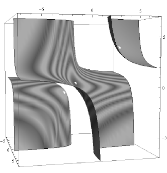
Figure 1: Cubic surface for case A1, with three Lorentz-invariant extrema.

To check this possibility, we construct numerically a three-dimensional plot of the cubic surface defined by the hamiltonian constraint (29), using the parameters $\overline{\beta}{}_{1}=0.3$, $\overline{\beta}{}_{2}=-1.3$, $\overline{\beta}{}_{3}=-1$, $\overline{\beta}{}_{4}=1$. See Fig. 1. The $x$, $y$, $z$ axes of the plot are labeled with values of $\lambda_{1}$, $\lambda_{2}$, $\lambda_{3}$, respectively. Equipotential contours of the effective potential $\overline{\mathcal{U}}{}(\lambda_{1},\lambda_{2})$ are displayed in grayscale shadings. The location of the three Lorentz-invariant extrema is indicated by white dots. Inspection of the figure reveals that the hamiltonian constraint involves three disconnected sheets, each containing a single stationary Lorentz-invariant extremum. This confirms that it is impossible to transit smoothly from one extremum to another. The two extrema in case A1 that represent local minima are therefore both locally and globally stable. Note, however, that the two globally stable extrema generically lie at different potentials. It follows that only the one at lower potential is absolutely stable. Since they are separated by infinite potential barriers, neither thermal fluctuations nor quantum tunneling between them can be expected to occur.

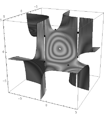
Figure 2: Cubic surface for case A2 and $\overline{\beta}{}_{3}^{2}-\overline{\beta}{}_{2}\overline{\beta}{}_{4}<0$, with one Lorentz-invariant extremum and six Lorentz-violating saddle points.

For case A2 with $D>0$ with one Lorentz-invariant extremum and six Lorentz-violating saddle points, the situation depends on the sign of the combination $\overline{\beta}{}_{3}^{2}-\overline{\beta}{}_{2}\overline{\beta}{}_{4}$. When $\overline{\beta}{}_{3}^{2}-\overline{\beta}{}_{2}\overline{\beta}{}_{4}<0$, the quadratic equation (41) has no real roots, so the cubic polynomial in (34) has no stationary points. The effective potential (50) consists of just one branch, as the denominator never becomes zero. Therefore, the solutions are connected by a path in the $\lambda_{i}$ space such that the effective potential $\overline{\mathcal{U}}{}$ varies continuously without passing through any singularity. This result is confirmed numerically in Fig. 2, which displays the cubic surface defined by the hamiltonian constraint for the parameters $\overline{\beta}{}_{1}=1$, $\overline{\beta}{}_{2}=-1$, $\overline{\beta}{}_{3}=1$, $\overline{\beta}{}_{4}=1$ using the same conventions as Fig. 1. The Lorentz-invariant extremum is indicated by a white dot, while the Lorentz-violating saddle points are indicated by black dots. We thus conclude that the Lorentz-invariant extremum at a local mininum is globally unstable. The excitation energy required to destabilize it is the difference between the energies of the Lorentz-violating saddle points and the Lorentz-invariant local minimum.

In contrast, when $\overline{\beta}{}_{3}^{2}-\overline{\beta}{}_{2}\overline{\beta}{}_{4}>0$, the analysis is more involved. The cubic equation (34) has two stationary points $\lambda_{-}$, $\lambda_{+}$ corresponding to the roots of the quadratic combination (46). Tne single root of the cubic equation must be either smaller than $\lambda_{-}$ or larger the $\lambda_{+}$. We now claim that this root for the Lorentz-invariant extremum and the two roots with $\lambda_{1}=\lambda_{2}$ for the Lorentz-violating saddle points are separated by $\lambda_{-}$ and $\lambda_{+}$, assuming the three roots are ordered from small to large.

To check this claim, we first evaluate the left-hand side $C$ of Eq. (34) at the centerpoint $(\lambda_{+}+\lambda_{-})/2$,

$$C=\frac{\overline{\beta}{}_{1}\overline{\beta}{}_{4}^{2}-3\overline{\beta}{}_{2}\overline{\beta}{}_{3}\overline{\beta}{}_{4}+2\overline{\beta}{}_{3}^{3}}{\overline{\beta}{}_{4}^{2}}.$$ (51)

It follows that if $\overline{\beta}{}_{4}C>0$ then the Lorentz-invariant root $\lambda_{\rm LI}$ is smaller than $\lambda_{-}$, while if $\overline{\beta}{}_{4}C<0$ then $\lambda_{\rm LI}$ is larger than $\lambda_{+}$. Next, we verify that the two Lorentz-violating roots $\lambda_{{\rm LV},-}$ and $\lambda_{{\rm LV},+}$ given in the solutions (42) are separated from $\lambda_{\rm LI}$ and each other by $\lambda_{-}$ and $\lambda_{+}$. If this is indeed the case, then either

$$\lambda_{LI}<\lambda_{-}<\lambda_{LV,-}<\lambda_{+}<\lambda_{LV,+}$$ (52)

or

$$\lambda_{LV,-}<\lambda_{-}<\lambda_{LV,+}<\lambda_{-}<\lambda_{LI}.$$ (53)

One consistency condition for this involves the sign of the difference between the midpoint of $\lambda_{LV,-}$ and $\lambda_{LV,+}$. Calculation reveals that the difference is given by

$$\frac{\lambda_{LV,-}+\lambda_{LV,-}}{2}-\frac{\lambda_{-}+\lambda_{+}}{2}=\frac{\overline{\beta}{}_{4}C}{\overline{\beta}{}_{3}^{2}-\overline{\beta}{}_{2}\overline{\beta}{}_{4}}.$$ (54)

Since $\overline{\beta}{}_{3}^{2}-\overline{\beta}{}_{2}\overline{\beta}{}_{4}>0$ for this case, we see that if $\overline{\beta}{}_{4}C>0$ then the midpoint between $\lambda_{LV,-}$ and $\lambda_{LV,+}$ is larger than $(\lambda_{+}+\lambda_{-})/2$, while if $\overline{\beta}{}_{4}C<0$ it is smaller. It therefore lies in the opposite direction from $\lambda_{LI}$ relative to $(\lambda_{+}+\lambda_{-})/2$, consistent with the claim.

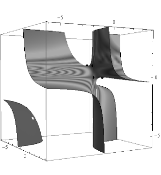
Figure 3: Cubic surface for case A2 and $\overline{\beta}{}_{3}^{2}-\overline{\beta}{}_{2}\overline{\beta}{}_{4}>0$, with one Lorentz-invariant extremum and six Lorentz-violating saddle points.

To confirm that the three roots are positioned according to the claim, we can compute explicitly the differences

$$\frac{\lambda_{+}-\lambda_{-}}{2}=\frac{\sqrt{\overline{\beta}{}_{3}^{2}-\overline{\beta}{}_{2}\overline{\beta}{}_{4}}}{|\overline{\beta}{}_{4}|}$$ (55)

and

$$\frac{\lambda_{LV,+}-\lambda_{LV,-}}{2}=\frac{\sqrt{D}}{2(\overline{\beta}{}_{3}^{2}-\overline{\beta}{}_{2}\overline{\beta}{}_{4})}.$$ (56)

The claim then follows if the conditions

$$\left|\frac{\overline{\beta}{}_{1}\overline{\beta}{}_{4}^{2}-3\overline{\beta}{}_{2}\overline{\beta}{}_{3}\overline{\beta}{}_{4}+2\overline{\beta}{}_{3}^{3}}{2\overline{\beta}{}_{4}(\overline{\beta}{}_{3}^{2}-\overline{\beta}{}_{2}\overline{\beta}{}_{4})}\right|-\frac{\sqrt{D}}{2(\overline{\beta}{}_{3}^{2}-\overline{\beta}{}_{2}\overline{\beta}{}_{4})}$$

$$\hskip 130.0pt>-\frac{\sqrt{\overline{\beta}{}_{3}^{2}-\overline{\beta}{}_{2}\overline{\beta}{}_{4}}}{|\overline{\beta}{}_{4}|},$$

$$\left|\frac{\overline{\beta}{}_{1}\overline{\beta}{}_{4}^{2}-3\overline{\beta}{}_{2}\overline{\beta}{}_{3}\overline{\beta}{}_{4}+2\overline{\beta}{}_{3}^{3}}{2\overline{\beta}{}_{4}(\overline{\beta}{}_{3}^{2}-\overline{\beta}{}_{2}\overline{\beta}{}_{4})}\right|-\frac{\sqrt{D}}{2(\overline{\beta}{}_{3}^{2}-\overline{\beta}{}_{2}\overline{\beta}{}_{4})}$$

$$\hskip 130.0pt<\frac{\sqrt{\overline{\beta}{}_{3}^{2}-\overline{\beta}{}_{2}\overline{\beta}{}_{4}}}{|\overline{\beta}{}_{4}|},$$

$$\left|\frac{\overline{\beta}{}_{1}\overline{\beta}{}_{4}^{2}-3\overline{\beta}{}_{2}\overline{\beta}{}_{3}\overline{\beta}{}_{4}+2\overline{\beta}{}_{3}^{3}}{2\overline{\beta}{}_{4}(\overline{\beta}{}_{3}^{2}-\overline{\beta}{}_{2}\overline{\beta}{}_{4})}\right|+\frac{\sqrt{D}}{2(\overline{\beta}{}_{3}^{2}-\overline{\beta}{}_{2}\overline{\beta}{}_{4})}$$

$$\hskip 130.0pt>\frac{\sqrt{\overline{\beta}{}_{3}^{2}-\overline{\beta}{}_{2}\overline{\beta}{}_{4}}}{|\overline{\beta}{}_{4}|}$$ (57)

all hold. Moving the second term in each of these relations to the right-hand side and squaring, we find that almost all terms cancel. All three inequalities reduce to

$$4(\overline{\beta}{}_{3}^{2}-\overline{\beta}{}_{2}\overline{\beta}{}_{4})^{3/2}|\overline{\beta}{}_{4}|\sqrt{D}>0,$$ (58)

which is valid by inspection. The claim that the three roots are separated by $\lambda_{-}$ and $\lambda_{+}$ is thus verified.

The above calculation therefore suggests that for case A2 with $D>0$ and $\overline{\beta}{}_{3}^{2}-\overline{\beta}{}_{2}\overline{\beta}{}_{4}>0$ the Lorentz-invariant stationary extremum and the two Lorentz-violating saddle points with $\lambda_{1}=\lambda_{2}$ lie on separate branches of the effective potential $\overline{\mathcal{U}}{}(\lambda_{1},\lambda_{2})$. A similar argument applies for the other four Lorentz-violating saddle points. However, the same caveat applies here as for case A1, as we considered only paths satisfying $\lambda_{1}=\lambda_{2}$. In fact, a graphical analysis reveals that continuous paths exist that link the six Lorentz-violating saddle points. This feature is manifest in Fig. 3, which plots the cubic surface defined by the hamiltonian constraint for the parameters $\overline{\beta}{}_{1}=1$, $\overline{\beta}{}_{2}=3$, $\overline{\beta}{}_{3}=1$, $\overline{\beta}{}_{4}=1$, with the conventions of Fig. 1. The Lorentz-invariant extremum indicated by a white dot lies on a disconnected component of the cubic surface, while the Lorentz-violating saddle points indicated by black dots are clustered around the throat of the other component. We see that a smooth transition from the Lorentz-invariant to the Lorentz-violating saddle points is impossible, so if the Lorentz-invariant extremum is a local minimum then it is also globally and absolutely stable. In contrast, smooth paths do indeed exist between any pair of Lorentz-violating saddle points.

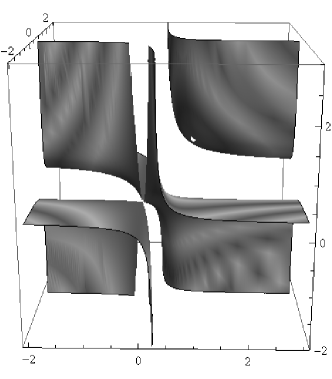
Figure 4: Cubic surface for the minimal theory in Ref. hr11 , with one Lorentz-invariant extremum.

As a final example, we consider the minimal theory obtained from the Fierz-Pauli Lagrange density by Hassan and Rosen hr11 . The corresponding the cubic surface defined by the hamiltonian constraint is displayed in Fig. 4 for the parameters $\overline{\beta}{}_{1}=\overline{\beta}{}_{2}=0$, $\overline{\beta}{}_{3}=-1$, $\overline{\beta}{}_{4}=3$, using the conventions of Fig. 1. These parameters yield $D=0$ and $\overline{\beta}{}_{3}^{2}-\overline{\beta}{}_{2}\overline{\beta}{}_{4}=1$, which is a limiting situation of the previous analysis. In this case, two sheets of the cubic surface touch at a conical singular point. The Lorentz-invariant extremum $\lambda_{0}=\lambda_{1}=\lambda_{2}=\lambda_{3}=0$ lies on the tip connecting the touching sheets and is unstable. In contrast, the Lorentz-invariant extremum $\lambda_{0}=\lambda_{1}=\lambda_{2}=\lambda_{3}=1$ is positioned on a disconnected component of the surface, as indicated by a white dot. It has a negative determinant of the bordered hessian and a positive value for the principal minor, so it is a local minimum that is globally and absolutely stable.

III.2 Case B: $\overline{\beta}{}_{4}=0$ and $\overline{\beta}{}_{3}\neq 0$

Consider next case B with $\overline{\beta}{}_{4}=0$, $\overline{\beta}{}_{3}\neq 0$. For rotationally invariant solutions with $\lambda_{1}=\lambda_{2}=\lambda_{3}$, reanalysis of Eqs. (29)–(33) reveals that the cubic (34) becomes replaced by the quadratic equation

$$\overline{\beta}{}_{1}+3\overline{\beta}{}_{2}\lambda_{1}+3\overline{\beta}{}_{3}\lambda_{1}^{2}=0,$$ (59)

which has solutions

$$\lambda_{1}=\frac{-\overline{\beta}{}_{2}\pm\sqrt{\overline{\beta}{}_{2}^{2}-\frac{4}{3}\overline{\beta}{}_{1}\overline{\beta}{}_{3}}}{2\overline{\beta}{}_{3}}.$$ (60)

From the first expression in Eq. (30) it follows that ${\widetilde{N}}=\lambda_{1}$, confirming that the extrema satisfy the condition (37) for Lorentz invariance. Note that they are real iff $3\overline{\beta}{}_{2}^{2}-4\overline{\beta}{}_{1}\overline{\beta}{}_{3}\geq 0$.

To investigate local stability of these extrema, we examine the determinant (45) of the bordered hessian and the principal minor (47). This shows that one extremum is a local maximum of the constrained effective potential $\overline{\mathcal{U}}{}$ while the other is a local minimum, depending on the sign of $\overline{\beta}{}_{2}+2\overline{\beta}{}_{3}\lambda_{1}$.

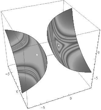
Figure 5: Double-sheeted hyperboloid for case B with two Lorentz-invariant extrema.

The effective potential in this case is the limit $\overline{\beta}{}_{4}\to 0$ of the expression (50). It is therefore singular along the curve satisfying

$$\overline{\beta}{}_{2}+\overline{\beta}{}_{3}(\lambda_{1}+\lambda_{2})=0.$$ (61)

The two Lorentz-invariant extrema are separated by this curve, so we expect them to lie on separate branches of the effective potential. This is confirmed by numerical analysis. The double-sheeted hyperboloid defined by the hamiltonian constraint is shown in Fig. 5 for the parameters $\overline{\beta}{}_{1}=1$, $\overline{\beta}{}_{2}=3$, $\overline{\beta}{}_{3}=1$, $\overline{\beta}{}_{4}=0$, using the conventions of Fig. 1. One of the two Lorentz-invariant extrema appears on each sheet, so they cannot be joined by a smooth curve on the surface. The extremum that is a local minimum of the potential is therefore globally and absolutely stable.

For solutions without rotational symmetry, Eqs. (31)–(33) require at least two of the $\lambda_{i}$ to be equal. Taking $\lambda_{1}=\lambda_{2}\neq\lambda_{3}$, we find that ${\widetilde{N}}=-\lambda_{1}-\overline{\beta}{}_{2}/\overline{\beta}{}_{3}$. Substitution into Eq. $(\ref{la_3-eom})$ then yields

$$\lambda_{1}=\lambda_{2}=\frac{-\overline{\beta}{}_{2}\pm\sqrt{4\overline{\beta}{}_{1}\overline{\beta}{}_{3}-3\overline{\beta}{}_{2}^{2}}}{2\overline{\beta}{}_{3}}.$$ (62)

Note that the solutions (60) are real iff $4\overline{\beta}{}_{1}\overline{\beta}{}_{3}-3\overline{\beta}{}_{2}^{2}\geq 0$, contrary to the situation for the Lorentz-invariant solutions. We also obtain

$$\lambda_{3}={\widetilde{N}}=\frac{-\overline{\beta}{}_{2}\mp\sqrt{4\overline{\beta}{}_{1}\overline{\beta}{}_{3}-3\overline{\beta}{}_{2}^{2}}}{2\overline{\beta}{}_{3}},$$ (63)

confirming that the solutions obey the condition (44) for Lorentz violation. Note that the roots of the solutions for $\lambda_{3}$ and ${\widetilde{N}}$ are interchanged relative to those for $\lambda_{1}$ and $\lambda_{2}$, as before. Two additional pairs of Lorentz-violating solutions are obtained by sequential interchange of $\lambda_{3}$ with $\lambda_{1}$ and with $\lambda_{2}$.

In this case, the determinant of the bordered hessian is obtained as the limit $\overline{\beta}{}_{4}\to 0$ of the expression (48),

$$\det H_{B}\to\bigl{(}3\overline{\beta}{}_{2}^{2}-\overline{\beta}{}_{1}\overline{\beta}{}_{3}\bigr{)}^{2}.$$ (64)

This is positive definite for $3\overline{\beta}{}_{2}^{2}-\overline{\beta}{}_{1}\overline{\beta}{}_{3}\neq 0$, so these solutions have a constrained hessian with one positive and one negative eigenvalue, corresponding to local saddle points of the effective potential.

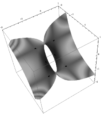
Figure 6: Single-sheeted hyperboloid for case B with six Lorentz-violating saddle points.

The Lorentz-violating saddle points are separated by the singular curve (61). However, numerical analysis reveals that all six saddle points lie on a unique branch of the effective potential. The hamiltonian constraint in this case defines a single-sheeted hyperboloid, shown in Fig. 6 for the parameters $\overline{\beta}{}_{1}=1$, $\overline{\beta}{}_{2}=1$, $\overline{\beta}{}_{3}=1$, $\overline{\beta}{}_{4}=0$ with the same conventions as Fig. 1. All six saddle points lie near the throat of the single-sheeted hyperboloid. Smooth transitions between all the saddle points are therefore possible.

III.3 Case C: $\overline{\beta}{}_{4}=\overline{\beta}{}_{3}=0$ and $\overline{\beta}{}_{2}\neq 0$

Finally, we consider case C with $\overline{\beta}{}_{4}=\overline{\beta}{}_{3}=0$, $\overline{\beta}{}_{2}\neq 0$. We find that a single Lorentz-invariant solution exists, given by

$${\widetilde{N}}=\lambda_{1}=\lambda_{2}=\lambda_{3}=-\overline{\beta}{}_{1}/(3\overline{\beta}{}_{2}).$$ (65)

This solution is a local minimum of the effective potential if $\overline{\beta}{}_{2}>0$ and a local maximum if $\overline{\beta}{}_{2}<0$. The solution set of the hamiltonian constraint is a single-sheeted plane, illustrated in Fig. 7 for the parameters $\overline{\beta}{}_{1}=1$, $\overline{\beta}{}_{2}=3$, $\overline{\beta}{}_{3}=\overline{\beta}{}_{4}=0$ using the same conventions as Fig. 1. As a result, if the extremum is a local minimum then it is globally and absolutely stable.

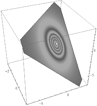
Figure 7: Single-sheeted plane for case C with a single Lorentz-invariant extremum.

Note that case C with a local minimum is the only scenario for which the potential remains bounded from below over the entire range of field variables. Branches of the effective potential that are unbounded below occur when the surface of the hamiltonian constraint contains a sheet with either a local maximum or a saddle point. This occurs for all situations in cases A and B and for case C with a local maximum. For these cases, a full quantum treatment may therefore be problematic as the path integral will probe degrees of freedom that correspond to a potential taking arbitrarily negative values. In this sense, even the existence of an absolutely stable extremum may be insufficient to guarantee stability at the quantum level for these cases. However, the parameter choices $\overline{\beta}{}_{4}=\overline{\beta}{}_{3}=0$, $\overline{\beta}{}_{2}>0$ for case C avoid this divergence and hence may be of particular interest in the quantum theory. At the classical level, in contrast, it suffices to restrict the theory via appropriate parameter choices to an individual sheet on which the potential is bounded from below, so the range of viable cases is correspondingly greater.

IV Linearized massive gravity

Varying the action (1) with respect to the metric $g_{\mu\nu}$ yields an equation of motion that can be written as hr11

$$G_{\mu\nu}+\frac{m^{2}}{2}\sum_{n=0}^{3}(-1)^{n}\beta_{n}\left(g_{\mu\alpha}Y^{\alpha}_{(n)\nu}+g_{\nu\alpha}Y^{\alpha}_{(n)\mu}\right)=\kappa T_{\mu\nu},$$ (66)

where $T^{\mu\nu}$ is the energy-momentum tensor and the tensors $Y^{\alpha}_{(n)\nu}$ are given in matrix form by

$$Y_{(n)}(\mathbb{X})=\sum_{k=0}^{n}(-1)^{k}\mathbb{X}^{n-k}e_{k}(\mathbb{X}).$$ (67)

We are interested in linearizing this equation around Minkowski spacetime with metric $\eta_{\mu\nu}$, while allowing for deviations $\delta f_{\mu\nu}$ of the fiducial metric $f_{\mu\nu}$ from $\eta_{\mu\nu}$. We therefore define

$$g_{\mu\nu}=\eta_{\mu\nu}+h_{\mu\nu},\quad f_{\mu\nu}=\eta_{\mu\nu}+\delta f_{\mu\nu},$$ (68)

and work at first order in both $h_{\mu\nu}$ and $f_{\mu\nu}$. To ensure the dynamical fluctuations $h_{\mu\nu}$ remain perturbative, we take $|h_{\mu\nu}|\ll|\delta f_{\mu\nu}|\ll 1$ where needed. The deviations $\delta f_{\mu\nu}$ are assumed to be constants. Note that the presence of the background Minkowski spacetime implies that $\delta f_{\mu\nu}$ can nonetheless produce physical effects, as a general coordinate transformation chosen to remove $\delta f_{\mu\nu}$ also changes the background metric to non-Minkowski form.

The square root $\mathbb{X}^{\mu}{}_{\nu}=(\sqrt{g^{-1}f}~{})^{\mu}{}_{\nu}$ can be expressed in terms of $h_{\mu\nu}$ and $f_{\mu\nu}$. The expansion

$$\mathbb{X}^{2} = (\eta+h)^{-1}(\eta+\delta f)$$ (69)

$$\approx \mathbb{1}+\eta^{-1}\delta f-\eta^{-1}h-\eta^{-1}h\,\eta^{-1}\delta f$$

implies

$$\mathbb{X}\approx\mathbb{1}+{\textstyle{\frac{1}{2}}}\eta^{-1}\delta f-\tfrac{1}{2}\eta^{-1}h+\tfrac{1}{8}\eta^{-1}\delta f\,\eta^{-1}h-\tfrac{3}{8}\eta^{-1}h\,\eta^{-1}\delta f.$$ (70)

The $n$th product of $\mathbb{X}$ then takes the form

$$\mathbb{X}^{n} \approx \mathbb{1}+\frac{n}{2}\left(\eta^{-1}\delta f-\eta^{-1}h\right)$$

$$\hskip-10.0pt-\tfrac{1}{8}\left[(n^{2}-2n)\eta^{-1}\delta f\,\eta^{-1}h+(n^{2}+2n)\eta^{-1}h\,\eta^{-1}\delta f\right].$$

The definition (67) contains the polynomial functions $e_{n}(\mathbb{X})$, which involve traces $[\mathbb{X}^{n}]$ of powers of $\mathbb{X}$. Taking the trace of Eq. (LABEL:X^n) yields

$$[\mathbb{X}^{n}]\approx 4+\frac{n}{2}\left([\eta^{-1}\delta f]-[\eta^{-1}h]\right)-\frac{n^{2}}{4}[\eta^{-1}\delta f\,\eta^{-1}h],$$ (72)

where the cyclic property of the trace has been used. Using this expression, we find the polynomial functions $e_{n}(\mathbb{X})$ take the form

$$e_{n}(\mathbb{X}) = \binom{4}{n}+\tfrac{1}{2}\binom{3}{n-1}\left([\eta^{-1}\delta f]-[\eta^{-1}h]\right)$$ (73)

$$-\tfrac{1}{4}\binom{2}{n-1}[\eta^{-1}\delta f\,\eta^{-1}h]$$

$$-\tfrac{1}{4}\binom{2}{n-2}[\eta^{-1}\delta f]\,[\eta^{-1}h].$$

Substituting the results (LABEL:X^n) and (73) in the definition (67) yields the form of $Y_{(n)}(\mathbb{X})$ at first order in the metric and the fiducial metric. The modified Einstein equation (66) becomes

$$G^{\rm L}_{\mu\nu}+\frac{m^{2}}{2}\sum_{n=0}^{3}\beta_{n}\biggl{\{}2\binom{3}{n}\bigl{(}\eta_{\mu\nu}+h_{\mu\nu}\bigr{)}+\binom{2}{n-1}\left(h_{\mu\nu}-\delta f_{\mu\nu}-\eta_{\mu\nu}\bigl{[}\eta^{-1}(h-\delta f)\bigr{]}\right)$$

$$\hskip 30.0pt+\left(\tfrac{1}{2}\binom{1}{n-2}+\binom{2}{n-1}\right)\bigl{[}\eta^{-1}\delta f\bigr{]}h_{\mu\nu}+\tfrac{1}{2}\binom{1}{n-2}\bigl{[}\eta^{-1}h\bigr{]}\delta f_{\mu\nu}$$

$$\hskip 30.0pt-\tfrac{1}{2}\binom{1}{n-1}\bigl{[}\eta^{-1}\delta f\,\eta^{-1}h\bigr{]}\eta_{\mu\nu}-\tfrac{1}{2}\binom{1}{n-2}\bigr{[}\eta^{-1}\delta f\bigr{]}\,\bigl{[}\eta^{-1}h\bigl{]}\eta_{\mu\nu}$$

$$\hskip 30.0pt-\left(\tfrac{3}{4}\binom{2}{n-1}-\tfrac{1}{2}\binom{1}{n-1}\right)\bigl{(}h\,\eta^{-1}\,\delta f+\delta f\,\eta^{-1}\,h\bigr{)}_{\mu\nu}\biggr{\}}=\kappa T_{\mu\nu},$$ (74)

where $G^{\rm L}_{\mu\nu}$ is the linearized Einstein tensor. This result represents the desired linearization of the dynamics.

It is reasonable and usual to require that the linearized equation (74) is satisfied by the choice $h_{\mu\nu}=\delta f_{\mu\nu}=T_{\mu\nu}=0$. This requirement constrains the parameters $\beta_{n}$ according to hir12

$$\sum_{n=0}^{3}\binom{3}{n}\beta_{n}=\beta_{0}+3\beta_{1}+3\beta_{2}+\beta_{3}=0.$$ (75)

Introducing now a nontrivial fluctuation $h_{\mu\nu}\neq 0$ while maintaining $\delta f_{\mu\nu}=T_{\mu\nu}=0$, the modified Einstein equation (74) becomes

$$G^{\rm L}_{\mu\nu}+\frac{m^{2}}{2}\sum_{n=0}^{3}\binom{2}{n-1}\beta_{n}\bigl{(}h_{\mu\nu}-[\eta^{-1}h]\bigr{)}=0.$$ (76)

If $\sum_{n=0}^{3}\binom{2-1}{n}\beta_{n}<0$, this equation describes tachyonic propagation and corresponds to an unstable system. If instead $\sum_{n=0}^{3}\binom{2}{n-1}\beta_{n}=0$, the mass term vanishes. We are thus interested in the case $\sum_{n=0}^{3}\binom{2}{n-1}\beta_{n}>0$. For this case, we can rescale the parameters $\beta_{n}\to a\beta_{n}$ and the mass $m\to m/\sqrt{a}$ so that $\sum_{n=0}^{3}\binom{2}{n-1}\beta_{n}\to 1$, thereby reducing the modified Einstein equation to the Fierz-Pauli equation. In what follows, we can therefore take

$$\sum_{n=0}^{3}\binom{2}{n-1}\beta_{n}=\beta_{1}+2\beta_{2}+\beta_{3}=1$$ (77)

without loss of generality. Note that the conditions (75) and (77) imply that only two combinations of the four parameters $\beta_{n}$ govern the physics of the system.

Suppose next that $\delta f_{\mu\nu}\neq 0$. Now Minkowski spacetime no longer solves the modified Einstein equation (74) when $T_{\mu\nu}=0$ because contributions from $\delta f$ to the mass term remain in the limit $h_{\mu\nu}\to 0$. This means that even in the absence of matter, $T_{\mu\nu}=0$, spacetime has nonzero curvature whenever $\delta f_{\mu\nu}$ is nonzero. The presence of this curvature complicates the form of solutions to the modified Einstein equation. To minimize the calculational complexities while still permitting study of relevant physical features, we can introduce a special constant background energy-momentum tensor chosen to cancel the $h_{\mu\nu}$-independent terms on the left-hand side of the modified Einstein equation,

$$\kappa T_{\mu\nu}=-\frac{m^{2}}{2}\left(\delta f_{\mu\nu}-\eta_{\mu\nu}[\eta^{-1}\delta f]\right).$$ (78)

Note that this is conserved in Minkowski spacetime for the spacetime-independent $\delta f_{\mu\nu}$ of interest here, and hence all its partial derivatives vanish. In the presence of this background, a zero metric fluctuation $h_{\mu\nu}=0$ solves the modified Einstein equation (74), and so spacetime is Minkowski. Nonzero solutions for $h_{\mu\nu}$ can then be interpreted in analogy with standard weak-field gravitational physics in GR, including gravitational waves in flat spacetime and the Newton gravitational potential.

To analyze the physics of this system, it is convenient to work in momentum space. We can write the linearized Einstein equation in the form

$$O_{\mu\nu}{}^{\alpha\beta}h_{\alpha\beta}=0$$ (79)

and introduce the Fourier transform

$$h_{\mu\nu}(x)=\int\frac{d^{4}p}{(2\pi)^{4}}e^{-ip\cdot x}{\widetilde{h}}_{\mu\nu}(p).$$ (80)

This yields the momentum-space equation of motion

$${\widetilde{O}}_{\mu\nu}{}^{\alpha\beta}{\widetilde{h}}_{\alpha\beta}=0,$$ (81)

where

$${\widetilde{O}}_{\mu\nu}{}^{\alpha\beta} = \left(\delta_{(\mu}^{\alpha}\delta_{\nu)}^{\beta}-\eta_{\mu\nu}\eta^{\alpha\beta}\right)(p^{2}+c_{1}m^{2})-2p_{(\mu}p^{(\alpha}\delta_{\nu)}^{\beta)}+p_{\mu}p_{\nu}\eta^{\alpha\beta}+\eta_{\mu\nu}p^{\alpha}p^{\beta}$$ (82)

$$+m^{2}\left(c_{2}\delta_{(\mu}^{(\alpha}\delta f_{\nu)}^{\beta)}+c_{3}[\eta^{-1}\delta f]\,\delta_{(\mu}^{\alpha}\delta_{\nu)}^{\beta}+c_{4}\left(\delta f_{\mu\nu}-\eta_{\mu\nu}[\eta^{-1}\delta f]\right)\eta^{\alpha\beta}+c_{5}\eta_{\mu\nu}\delta f^{\alpha\beta}\right),$$

with

$$c_{1} = \sum_{n}\beta_{n}\binom{2}{n-1},\quad c_{2}=-\tfrac{3}{2}c_{1}+\sum_{n}\beta_{n}\binom{1}{n-1},$$

$$c_{3} = \tfrac{3}{4}c_{1}-\tfrac{1}{2}c_{2},\quad c_{4}=-\tfrac{1}{4}c_{1}-\tfrac{1}{2}c_{2},\quad c_{5}=-\tfrac{3}{4}c_{1}-\tfrac{1}{2}c_{2}.$$

It is convenient to scale $m$ so that $c_{1}=1$. The only remaining independent parameter is then $c_{2}$. The first four terms in expression (82) reproduce the usual Fierz-Pauli result fp39 , as expected. The tensor ${\widetilde{O}}_{\mu\nu}{}^{\alpha\beta}$ satisfies the symmetry properties

$${\widetilde{O}}_{\mu\nu}{}^{\alpha\beta}={\widetilde{O}}_{\nu\mu}{}^{\alpha\beta}={\widetilde{O}}_{\mu\nu}{}^{\beta\alpha}.$$ (84)

Note, however, that ${\widetilde{O}}_{\mu\nu\alpha\beta}\neq{\widetilde{O}}_{\alpha\beta\mu\nu}$ whenever $\delta f_{\mu\nu}$ is nonzero.

IV.1 Gravitational waves

In this section, we consider the application of the linearized theory of massive gravity to the propagation of gravitational waves. We first summarize the situation for $\delta f_{\mu\nu}=0$, which corresponds to the Fierz-Pauli limit in Minkowski spacetime, and then turn to the scenario with $\delta f_{\mu\nu}\neq 0$.

For $\delta f_{\mu\nu}=0$, contracting the expression (81) with $p^{\nu}$ and $\eta^{\mu\nu}$ in turn shows that it is equivalent to the conditions

$${\widetilde{h}}_{\mu\alpha}p^{\alpha}=0,\quad{\widetilde{h}}_{\mu}{}^{\mu}=0,\quad(p^{2}+m^{2}){\widetilde{h}}_{\mu\nu}=0.$$ (85)

This set of equations represents five constraints on the 10 components of ${\widetilde{h}}_{\mu\nu}$ together with the usual dispersion relation $p^{2}=-m^{2}$ for the five independent combinations. The conditions and the dispersion relation are both particle and observer Lorentz covariant, and the five independent combinations correspond to the five physical helicities of a massive spin-2 field.

The five constraint equations can be solved explicitly by taking advantage of observer Lorentz invariance to choose an observer frame in which the 4-momentum takes the form

$$p^{\mu}=\bigl{(}E;0,0,p_{3}\bigr{)}$$ (86)

with $E=\sqrt{m^{2}+p_{3}^{2}}$. The particle Lorentz invariance of the system guarantees that the physical behavior is unchanged for other momentum choices in this chosen observer frame. The five constraint equations in Eq. (85) can then be satisfied by choosing the five independent variables as ${\widetilde{h}}_{11}$, ${\widetilde{h}}_{22}$, ${\widetilde{h}}_{12}$, ${\widetilde{h}}_{13}$, ${\widetilde{h}}_{23}$ and expressing the remaining five components of ${\widetilde{h}}_{\mu\nu}$ in terms of them,

$${\widetilde{h}}_{01} = \frac{p_{3}}{E}{\widetilde{h}}_{13},\quad{\widetilde{h}}_{02}=\frac{p_{3}}{E}{\widetilde{h}}_{23},$$

$${\widetilde{h}}_{03} = -\frac{E}{p_{3}}{\widetilde{h}}_{00}=-\frac{p_{3}}{E}{\widetilde{h}}_{33}=\frac{E\,p_{3}}{m^{2}}\bigl{(}{\widetilde{h}}_{11}+{\widetilde{h}}_{22}\bigr{)}.$$ (87)

To obtain the helicity eigenstates, we consider a rotation about the three momentum $\vec{p}$ given by the Lorentz transformation

$$h^{\prime}_{\mu\nu}=R_{\mu}{}^{\alpha}R_{\nu}{}^{\beta}{\widetilde{h}}_{\alpha\beta},$$ (88)

with

$$R_{\mu}{}^{\alpha}=\begin{pmatrix}1&0&0&0\\ 0&\cos\theta&\sin\theta&0\\ 0&-\sin\theta&\cos\theta&0\\ 0&0&0&1\end{pmatrix}.$$ (89)

By definition, a state $\psi_{n}$ of helicity $n$ then transforms according to

$$\psi^{\prime}_{n}=e^{in\theta}\psi_{n}.$$ (90)

Calculation with these expressions reveals that the helicity eigenstates of ${\widetilde{h}}_{\mu\nu}$ satisfying the conditions (87) are given by

$${\widetilde{h}}^{(\pm 2)}_{\mu\nu} =\frac{m^{2}}{2}\begin{pmatrix}0&0&0&0\\ 0&1&\pm i&0\\ 0&\pm i&-1&0\\ 0&0&0&0\end{pmatrix},$$

$${\widetilde{h}}^{(\pm 1)}_{\mu\nu} =\begin{pmatrix}0&p_{3}&\mp ip_{3}&0\\ p_{3}&0&0&-E\\ \mp ip_{3}&0&0&\pm iE\\ 0&-E&\pm iE&0\end{pmatrix},$$

$${\widetilde{h}}^{(0)}_{\mu\nu} =\begin{pmatrix}p_{3}^{2}&0&0&-p_{3}E\\ 0&-m^{2}/2&0&0\\ 0&0&-m^{2}/2&0\\ -p_{3}E&0&0&E^{2}\end{pmatrix}.$$ (91)

As expected, the five physical degrees of freedom of the massive spin-2 field include two helicity-2 components ${\widetilde{h}}^{(\pm 2)}_{\mu\nu}$, two helicity-1 components ${\widetilde{h}}^{(\pm 1)}_{\mu\nu}$, and a helicity-0 component ${\widetilde{h}}^{(0)}_{\mu\nu}$. Each component obeys the Lorentz-invariant dispersion relation appropriate for a particle of mass $m$.

IV.1.1 Analysis in special observer frame

Next, we consider effects of the terms proportional to $\delta f_{\mu\nu}$ in the equation of motion (81). Selecting a special observer frame in which the 4-momentum takes the form (86) and contracting the equation of motion with $p^{\nu}$ and $\eta^{\mu\nu}$ in turn, five constraints again emerge. Working at first order in $\delta f_{\mu\nu}$, calculation reveals they can be cast in the form

$${\widetilde{h}}_{\mu\alpha}p^{\alpha} = \tfrac{1}{3}p_{\mu}[\eta^{-1}\delta f\eta^{-1}{\widetilde{h}}]\left(c_{2}+c_{4}\left(1-2\frac{p^{2}}{m^{2}}\right)\right)$$

$$-\tfrac{1}{2}c_{2}p^{\alpha}\delta f_{\alpha}{}^{\beta}{\widetilde{h}}_{\beta\mu},$$

$${\widetilde{h}}_{\alpha}{}^{\alpha} = \tfrac{1}{3}[\eta^{-1}\delta f\eta^{-1}{\widetilde{h}}]\left(c_{2}+c_{4}\left(4-2\frac{p^{2}}{m^{2}}\right)\right),\quad$$ (92)

which generalizes the five constraints in Eq. (85). Combining these results with the equation of motion (81) permits the latter to be expressed in the simplified form

$$\bigl{(}p^{2}+m^{2}(1+c_{3}[\eta^{-1}\delta f])\bigr{)}{\widetilde{h}}_{\mu\nu}=$$

$$\hskip 20.0pt\frac{m^{2}}{2}c_{2}\,\bigl{(}{\widetilde{h}}_{\mu\alpha}\delta f^{\alpha}{}_{\nu}+\delta f_{\mu\alpha}{\widetilde{h}}^{\alpha}{}_{\nu}\bigr{)}+c_{2}\,p^{\alpha}\delta f_{\alpha}{}^{\beta}{\widetilde{h}}_{\beta(\mu}p_{\nu)}$$

$$\hskip 60.0pt-\frac{c_{2}}{3}[\eta^{-1}\delta f\eta^{-1}{\widetilde{h}}]\bigl{(}p_{\mu}p_{\nu}+m^{2}\eta_{\mu\nu}\bigr{)},$$ (93)

generalizing the dispersion relation in Eq. (85).

Inspection reveals that the parameter $c_{3}$ governs an overall mass shift set by the $\eta_{\mu\nu}$-trace of the fluctuation $\delta f_{\mu\nu}$ of the fiducial metric. The role of the terms on the right-hand side of the modified dispersion relation (93) involves a nontrivial action on the components of ${\widetilde{h}}_{\mu\nu}$, so their physical content appears more challenging to understand. However, the structure of the modified dispersion relation implies that it can be interpreted as an eigenvalue equation, as the combined action of the $c_{2}$ terms must be proportional to ${\widetilde{h}}_{\mu\nu}$. The physical content of the system is therefore determined by the eigenvalues and eigenfunctions of Eq. (93), with ${\widetilde{h}}_{\mu\nu}$ constrained to satisfy the conditions (92). Note that $E$ can be taken approximately equal to its unperturbed value $\sqrt{m^{2}+p_{3}^{2}}$ in evaluating the action of the $c_{2}$ terms at first order in $\delta f_{\mu\nu}$.

To gain insight into the physics and for simplicity, we suppose first that $\delta f_{\mu\nu}$ has the diagonal form

$$\delta f_{\mu\nu}=\begin{pmatrix}a&0&0&0\\ 0&b_{1}&0&0\\ 0&0&b_{2}&0\\ 0&0&0&b_{3}\end{pmatrix}.$$ (94)

Calculation then reveals five distinct eigenvalues for the $c_{2}$ terms on the right-hand side of Eq. (93),

$$\lambda_{12} = -\frac{c_{2}}{2}m^{2}(b_{1}+b_{2}),\quad\lambda_{13}=-\frac{c_{2}}{2}\bigl{(}m^{2}(b_{1}+b_{3})+p_{3}^{2}(a+b_{3})\bigr{)},\quad\lambda_{23}=-\frac{c_{2}}{2}\bigl{(}m^{2}(b_{2}+b_{3})+p_{3}^{2}(a+b_{3})\bigr{)}$$

$$\lambda_{\pm} = -\frac{c_{2}}{3}\Biggl{(}(b_{1}+b_{2}+b_{3})m^{2}+(a+b_{3})p_{3}^{2}\pm\sqrt{\left(m^{2}\left(b_{3}-\frac{b_{1}+b_{2}}{2}\right)+p_{3}^{2}(a+b_{3})\right)^{2}+\frac{3}{4}(b_{1}-b_{2})^{2}m^{4}}\,\Biggr{)}.$$ (95)

For the energy eigenvalue $p_{0}$, the modified dispersion relation yields

$$p_{0} = \sqrt{p_{3}^{2}+m^{2}\bigl{(}1-c_{3}[\eta^{-1}\delta f]\bigr{)}+\lambda}\approx\sqrt{p_{3}^{2}+m^{2}}\left(1-\frac{m^{2}c_{3}[\eta^{-1}\delta f]+\lambda}{2\bigl{(}p_{3}^{2}+m^{2}\bigr{)}}\right),$$ (96)

where $\lambda$ takes the values (95). We thus see that the energy degeneracy between the five helicities in the Fierz-Pauli limit becomes broken when $\delta f_{\mu\nu}\neq 0$.

At leading order in $\delta f_{\mu\nu}$, the eigenstates corresponding to the eigenvalues $\lambda_{12}$, $\lambda_{13}$, $\lambda_{23}$ are the components ${\widetilde{h}}_{12}$, ${\widetilde{h}}_{13}$, ${\widetilde{h}}_{23}$, respectively. The eigenstates corresponding to $\lambda_{\pm}$ are linear combinations of ${\widetilde{h}}_{11}$ and ${\widetilde{h}}_{22}$, with parameters depending on $m$, $f_{\mu\nu}$, and $p_{3}$. These eigenstates differ from the helicity eigenstates (91) of the Fierz-Pauli spin-2 theory, instead being nontrivial linear combinations of the latter. The remaining components of ${\widetilde{h}}_{\mu\nu}$ are defined by Eqs. (87).

The situation simplifies in the ultra-relativistic limit $p_{3}\gg m$. The energy shifts corresponding to the eigenvalues $\lambda_{13}$ and $\lambda_{23}$ then become equal. The same holds for the shifts corresponding to $\lambda_{12}$ and $\lambda_{-}$. As a result, the five distinct energy eigenvalues merge into only three. Moreover, the corresponding eigenstates reduce to the helicity eigenstates (91). Explicitly, we find

$$\frac{p_{0}}{\sqrt{p_{3}^{2}+m^{2}}}\longrightarrow\begin{cases}1&\text{for helicities}\pm 2,\\ 1-\tfrac{1}{4}c_{2}(a+b_{3})&\text{for helicities}\pm 1,\\ 1-\tfrac{1}{3}c_{2}(a+b_{3})&\text{for helicity }0\end{cases}$$ (97)

in the ultrarelativistic limit.

Overall, the above treatment provides intriguing physical insight into the behavior of the gravitational waves when $\delta f_{\mu\nu}\neq 0$. In general, the energies of the five modes of the massive graviton undergo splitting. This corresponds to a lifting of the degeneracy of the graviton spectrum, and it generates ‘pentarefringence’ or ‘quinquerefringence’ in propagating gravitational waves. The pentarefringence reduces to ‘trirefringence’ in the ultrarelativistic limit.

The pentarefringent behavior of massive gravitational waves is analogous to the birefringence of electromagnetic waves known to occur in Minkowski spacetime in the presence of background coefficients for Lorentz violation km09 . The latter effects are detectable in suitable electromagnetic experiments. Although outside the scope of the present work, it would be of definite interest to investigate the prospects of experimentally measuring the pentarefringence of gravitational waves with existing and future detectors.

Table 1: Eigenvalues and eigenfunctions for special cases.

Condition	Eigenvalue	Eigenfunction
$C^{\pm}=0$	${\textstyle{\frac{1}{2}}}A+B$	$\dfrac{D^{-}}{D^{+}}h^{(2)}-\dfrac{A-2B}{2D^{+}}h^{(1)}-3h^{(0)}-\dfrac{A-2B}{2D^{-}}h^{(-1)}+\dfrac{D^{+}}{D^{-}}h^{(2)}$
	$\lambda_{\pm}\equiv\tfrac{1}{3}({2(A+B)\pm\sqrt{(A-2B)^{2}+12D^{+}D^{-}}})$	$\dfrac{D^{-}}{D^{+}}h^{(2)}+\dfrac{\lambda_{\pm}-A}{D^{+}}h^{(1)}-\Bigl{(}\dfrac{\left(B-{\textstyle{\frac{1}{2}}}A\right)(\lambda_{\pm}-A)}{D^{+}D^{-}}+1\Bigr{)}h^{(0)}$
		$\qquad+\dfrac{\lambda_{\pm}-A}{D^{-}}h^{(-1)}+\dfrac{D^{+}}{D^{-}}h^{(2)}$
	$\lambda_{\pm}\equiv\tfrac{1}{4}({3A+2B\pm\sqrt{(A-2B)^{2}+12D^{+}D^{-}}})$	$\dfrac{D^{-}}{D^{+}}h^{(2)}-\dfrac{\lambda_{\pm}-A-B}{D^{+}}h^{(1)}+\dfrac{\lambda_{\pm}-A-B}{D^{-}}h^{(-1)}-\dfrac{D^{+}}{D^{-}}h^{(2)}$
$D^{\pm}=0$	$A$	$C^{-}h^{(2)}-C^{+}h^{(-2)}$
	$\frac{1}{2}A+B\pm\frac{1}{2}\sqrt{C^{+}C^{-}}$	$C^{-}h^{(1)}\pm C^{+}h^{(-1)}$
	$\lambda_{\pm}\equiv\frac{2}{3}(A+B)\pm\frac{1}{3}\sqrt{(A-2B)^{2}+3C^{+}C^{-}}$	$C^{-}h^{(2)}+3(A-\lambda_{\pm})h^{(0)}+C^{+}h^{(-2)}$
$C^{\pm},D^{\pm}\to 0$	$-2b$	$h^{(\pm 2)}$
	$-2b-(a+b)\dfrac{|\vec{p}|^{2}}{m^{2}}$	$h^{(\pm 1)}$
	$-2b-\frac{4}{3}(a+b)\dfrac{|\vec{p}|^{2}}{m^{2}}$	$h^{(0)}$

IV.1.2 Analysis in a general helicity frame

The treatment in the previous subsection is limited by the fixed value (86) of the momentum in the chosen frame and by the special form (94) adopted for the fluctuation $\delta f_{\mu\nu}$ of the fiducial metric. Next, we extend the analysis and study the persistence of the pentarefringence effect in the general case.

Consider first an arbitrary momentum $p^{\mu}=\bigl{(}E;\vec{p}\bigr{)}$ in a generic observer frame, where $E=\sqrt{m^{2}+|\vec{p}|^{2}}$. To describe the corresponding helicity eigenstates, it is convenient to define the quantity

$$\overline{p}{}^{\mu}=\bigl{(}|\vec{p}|;E\frac{\vec{p}}{|\vec{p}|}\,\bigr{)}.$$ (98)

Provided $\vec{p}\neq 0$, which we assume to hold in what follows, this quantity is well defined and transforms as the 4-momentum of a particle with mass squared $-m^{2}$. We also define two other purely spacelike four-vectors,

$$e_{1}^{\mu}=\bigl{(}0;\vec{e}_{1}\bigr{)},\quad e_{2}^{\mu}=\bigl{(}0;\vec{e}_{2}\bigr{)},$$ (99)

where $\vec{e}_{1}$ and $\vec{e}_{2}$ are taken to have norm $m$, to be mutually orthogonal, and to be orthogonal to $\vec{p}$ such that the triple $\{\vec{e}_{1},\vec{e}_{2},\vec{p}\}$ represents a right-handed set of orthogonal basis vectors. The four 4-vectors $p^{\mu}$, $\overline{p}{}^{\mu}$, $e_{1}^{\mu}$, $e_{2}^{\mu}$ then form a nondegenerate basis satisfying the relations

$$p\cdot\overline{p}{} = p\cdot e_{1}=p\cdot e_{2}=0,$$

$$\overline{p}{}\cdot e_{1} = \overline{p}{}\cdot e_{2}=e_{1}\cdot e_{2}=0,$$

$$\overline{p}{}\cdot\overline{p}{} = e_{1}\cdot e_{1}=e_{2}\cdot e_{2}=-p^{2}=m^{2}.$$ (100)

Using this basis, the helicity eigenstates (91) for general momentum can be expressed as

$${\widetilde{h}}^{(\pm 2)}_{\mu\nu} = \frac{1}{2}\bigl{(}e_{1\,\mu}e_{1\,\nu}-e_{2\,\mu}e_{2\,\nu}\bigr{)}\mp ie_{1\,(\mu}e_{2\,\nu)},$$

$${\widetilde{h}}^{(\pm 1)}_{\mu\nu} = \bigl{(}e_{(\mu}\mp ie_{2\,(\mu}\bigr{)}\overline{p}{}_{\nu)},$$

$${\widetilde{h}}^{(0)}_{\mu\nu} = \overline{p}{}_{\mu}\overline{p}{}_{\nu}-\frac{1}{2}e_{1\,\mu}e_{1\,\nu}-\frac{1}{2}e_{2\,\mu}e_{2\,\nu}.$$ (101)

With these eigenstates in hand, we can revisit the determination of the eigenvalues and eigenvectors of the dispersion relation (93), allowing now for an arbitrary momentum $p^{\mu}$ and a general form for the fluctuation $\delta f_{\mu\nu}$. Excluding the common factor $c_{2}m^{2}/2$, the terms on the right-hand side of the dispersion relation can be written as an operator $S_{\mu\nu}{}^{\alpha\beta}$ acting on ${\widetilde{h}}_{\alpha\beta}$,

$$S_{\mu\nu}{}^{\alpha\beta}{\widetilde{h}}_{\alpha\beta} = {\widetilde{h}}_{\mu\alpha}\delta f^{\alpha}{}_{\nu}+\delta f_{\mu\alpha}{\widetilde{h}}^{\alpha}{}_{\nu}+\frac{2}{m^{2}}p^{\alpha}\delta f_{\alpha}{}^{\beta}{\widetilde{h}}_{\beta(\mu}p_{\nu)}$$ (102)

$$-\frac{2}{3m^{2}}[\eta^{-1}\delta f\eta^{-1}{\widetilde{h}}]\bigl{(}p_{\mu}p_{\nu}+m^{2}\eta_{\mu\nu}\bigr{)}.$$

Some algebra then reveals explicit expressions for the action of $S_{\mu\nu}{}^{\alpha\beta}$ on the helicity eigenstates (101),

$$S_{\mu\nu}{}^{\alpha\beta}{\widetilde{h}}^{(\pm 2)}_{\alpha\beta} = A{\widetilde{h}}^{(\pm 2)}_{\mu\nu}+D^{\mp}{\widetilde{h}}^{(\pm 1)}_{\mu\nu}-\frac{1}{3}{\widetilde{h}}^{(0)}_{\mu\nu},$$

$$S_{\mu\nu}{}^{\alpha\beta}{\widetilde{h}}^{(\pm 1)}_{\alpha\beta} = D^{\mp}{\widetilde{h}}^{(\pm 2)}_{\mu\nu}+\frac{2B+A}{2}{\widetilde{h}}^{(\pm 1)}_{\mu\nu}$$

$$+\frac{1}{3}D^{\mp}{\widetilde{h}}^{(0)}_{\mu\nu}+\frac{1}{2}C^{\mp}{\widetilde{h}}^{(\mp 1)}_{\mu\nu},$$

$$S_{\mu\nu}{}^{\alpha\beta}{\widetilde{h}}^{(0)}_{\alpha\beta} = -\frac{1}{2}C^{+}{\widetilde{h}}^{(2)}_{\mu\nu}+\frac{1}{2}D^{+}{\widetilde{h}}^{(1)}_{\mu\nu}+\frac{4B+A}{3}{\widetilde{h}}^{(0)}_{\mu\nu}$$ (103)

$$+\frac{1}{2}D^{-}{\widetilde{h}}^{(-1)}_{\mu\nu}-\frac{1}{2}C^{-}{\widetilde{h}}^{(-2)}_{\mu\nu}.$$

In these results, the momentum-dependent dimensionless quantities $A$, $B$, $C^{\pm}$, $D^{\pm}$ represent linear combinations of the matrix elements of the tensor $\delta f$ expressed in the basis spanned by $p^{\mu}$, $\overline{p}{}^{\mu}$, $e_{1}^{\mu}$, $e_{2}^{\mu}$,

$$A = -\frac{1}{m^{2}}\bigl{(}e_{1}\cdot\delta f\cdot e_{1}+e_{2}\cdot\delta f\cdot e_{2}\bigr{)},$$

$$B = -\frac{1}{m^{2}}\,\overline{p}{}\cdot\delta f\cdot\overline{p}{},$$

$$C^{\pm} = -\frac{1}{m^{2}}\bigl{(}e_{1}\cdot\delta f\cdot e_{1}-e_{2}\cdot\delta f\cdot e_{2}\pm 2ie_{1}\cdot\delta f\cdot e_{2}\bigr{)},$$

$$D^{\pm} = -\frac{1}{m^{2}}\bigl{(}e_{1}\cdot\delta f\cdot\overline{p}{}\pm ie_{2}\cdot\delta f\cdot\overline{p}{}\bigr{)}.$$ (104)

Note that $C^{-}=(C^{+})^{*}$ and $D^{-}=(D^{+})^{*}$.

Using Eq. (103), we find that the operator $S_{\mu\nu}{}^{\alpha\beta}/{2m^{2}}$ has five eigenvalues that generically are distinct. Two of them can be written as

$$\lambda_{\pm}=\tfrac{2}{3}(A+B)\pm\tfrac{1}{3}\sqrt{(A-2B)^{2}+3C^{+}C^{-}+12D^{+}D^{-}},$$ (105)

while the other three are the roots of the cubic polynomial

$$4\lambda^{3}-8(A+B)\lambda^{2}$$

$$\quad+(5A^{2}+12AB+4B^{2}-C^{+}C^{-}-D^{+}D^{-})\lambda$$

$$\quad-A^{3}-4A^{2}B-4AB^{2}+AC^{+}C^{-}+2(A+2B)D^{+}D^{-}$$

$$\quad+C^{+}(D^{-})^{2}+C^{-}(D^{+})^{2}=0.$$ (106)

These results establish the splitting of the energies of the five modes for the general case and hence confirm that gravitational waves in the theory undergo pentarefringence during propagation.

The eigenfunctions for the five modes can also be found by explicit calculation. Their expressions are lengthy, so we provide here for reference only the results for two special cases for which the results are substantially simplified. The first case is the scenario with $C^{\pm}=0$, while the second is the case with $D^{\pm}=0$. Table 1 displays the corresponding eigenvalues and eigenfunctions for these two cases.

To gain further physical insight, consider an explicit example for which the fluctuation $\delta f_{\mu\nu}$ takes a comparatively simple form in the chosen observer frame,

$$\delta f_{00}=a,\quad\delta f_{ii}=b,\quad i=1,2,3,$$ (107)

with other components of $\delta f_{\mu\nu}$ being zero. Writing the 4-momentum components as $p^{\mu}=(E;p_{1},p_{2},p_{3})$ and assuming $p_{2}^{2}+p_{3}^{2}\neq 0$, we can choose the basis vectors (99) to be

$$\vec{e}_{1} = \bigl{(}0,p_{3},-p_{2}\bigr{)}\frac{m}{\sqrt{p_{2}^{2}+p_{3}^{2}}},$$

$$\vec{e}_{2} = \bigl{(}-p_{2}^{2}-p_{3}^{2},p_{1}p_{2},p_{1}p_{3}\bigr{)}\frac{m}{|\vec{p}|\sqrt{p_{2}^{2}+p_{3}^{2}}}.$$ (108)

If $p_{2}^{2}+p_{3}^{2}=0$, then an alternative choice is possible instead, with the physical conclusions below being unaffected.

In this example, the linear combinations (104) are found to have the explicit forms

$$A=-2b,\quad B=-b-(a+b)\frac{|\vec{p}|^{2}}{m^{2}},\quad C^{\pm}=D^{\pm}=0.$$ (109)

Using the results displayed in Table 1 for the cases $C^{\pm}=0$ and $D^{\pm}=0$, we can identify the eigenvalues of the operator $S_{\mu\nu}{}^{\alpha\beta}$. The limit $C^{\pm}\to 0$, $D^{\pm}\to 0$ can be obtained with some care from either case, along with the corresponding eigenfunctions of $S_{\mu\nu}{}^{\alpha\beta}$. The results are listed in the last three rows of Table 1. The eigenfunctions turn out to coincide exactly with the helicity eigenstates. The eigenvalues for the helicities $\pm 1$ are degenerate, as are those for helicities $\pm 2$.

The dispersion relation (93) yields the corresponding energies as

$$E=\begin{cases}\sqrt{|\vec{p}|^{2}+m^{2}\bigl{(}1+c_{3}(a-3b)-c_{2}b\bigr{)}}&\text{for helicity }\pm 2,\\ \sqrt{|\vec{p}|^{2}\bigl{(}1-\frac{1}{2}c_{2}(a+b)\bigr{)}+m^{2}\bigl{(}1+c_{3}(a-3b)-c_{2}b\bigr{)}}&\text{for helicity }\pm 1,\\ \sqrt{|\vec{p}|^{2}\bigl{(}1-\frac{2}{3}c_{2}(a+b)\bigr{)}+m^{2}\bigl{(}1+c_{3}(a-3b)-c_{2}b\bigr{)}}&\text{for helicity }0,\end{cases}$$ (110)

revealing triplet splitting. Gravitational waves therefore experience trirefringence in this example. As expected, all helicities experience a mass shift $\delta m$ obeying $\delta m^{2}=m^{2}\bigl{(}c_{3}(a-3b)-c_{2}b\bigr{)}$. The helicities $\pm 1$ and 0 also undergo a shift in momentum dependence, which modifies their group velocities. Introducing the notation $\hat{p}=\vec{p}/|\vec{p}|$, we find the explicit group velocities are given by

$$\vec{v}_{g}=\frac{\partial E}{\partial\vec{p}}=\begin{cases}\dfrac{\vec{p}}{E}\quad\overset{|\vec{p}|\to\infty}{\longrightarrow}\quad\hat{p}&\text{for helicity }\pm 2,\\ \bigl{(}1-\frac{1}{2}c_{2}(a+b)\bigr{)}\dfrac{\vec{p}}{E}\quad\overset{|\vec{p}|\to\infty}{\longrightarrow}\quad\sqrt{1-\frac{1}{2}c_{2}(a+b)}\,\hat{p}&\text{for helicity }\pm 1,\\[6.0pt] \bigl{(}1-\frac{2}{3}c_{2}(a+b)\bigr{)}\dfrac{\vec{p}}{E}\quad\overset{|\vec{p}|\to\infty}{\longrightarrow}\quad\sqrt{1-\frac{2}{3}c_{2}(a+b)}\,\hat{p}\qquad&\text{for helicity }0,\end{cases}$$ (111)

where the expression for $E$ in each case is given by the corresponding result in Eq. (110).

The results (111) offer additional physical insight into the nature of the wave propagation. For the fluctuation $\delta f_{\mu\nu}$ of the fiducial metric to be small relative to $\eta_{\mu\nu}$ as required in the definition (68), it follows that $|a|$ and $|b|$ must satisfy $|a|,|b|\ll 1$. When the 3-momentum is also small, $|\vec{p}|\lesssim m$, the group velocities (111) are then always below unity and the 4-momenta are always timelike, so both microcausality and energy positivity hold. In the ultrarelativistic limit, however, inspection of the group velocities (111) reveals that in all cases the magnitude of the group velocity obeys

$$|\vec{v}_{g}|\overset{|\vec{p}|\to\infty}{\longrightarrow}\frac{E}{|\vec{p}|}.$$ (112)

This implies that for $|\vec{p}|\gg m$ the group velocities tend from below to the values $1$, $\sqrt{1-\frac{1}{2}c_{2}(a+b)}$, and $\sqrt{1-\frac{2}{3}c_{2}(a+b)}$ for helicities $\pm 2$, $\pm 1$, and 0, respectively. Therefore, when $c_{2}(a+b)>0$ the group velocities will be subluminal for any value of the momentum, assuring microcausality. However, the unconventional momentum dependence for the helicities $\pm 1$ and 0 implies that in this case the corresponding 4-momenta asymptote at high $|\vec{p}|$ to a spacelike cone in 4-momentum space and hence become spacelike, so observer frames can be found where the energies are negative. In constrast, when $c_{2}(a+b)<0$ the group velocities of the helicities $\pm 1$ and 0 become superluminal at sufficiently high $|\vec{p}|$ and so violate microcausality, but the 4-momenta then asymptote to a timelike cone in 4-momentum space and hence remain timelike in any observer frame. This complementary behavior of microcausality and energy positivity is analogous to that displayed by the dispersion relation for a Lorentz-violating Dirac spinor with positive coefficient $c_{00}$, as discussed in Sec. IV C of Ref. kl01 . The superluminal features found here may parallel results concerning superluminal modes in ghost-free gravity obtained via other approaches ag11 ; diow13 ; frhm13 .

We can confirm the generality of the above physical interpretations by replacing the special fluctuation (107) of the fiducial metric with the form

$$\delta f_{\mu\nu}=\begin{pmatrix}a&\delta f_{01}&\delta f_{02}&\delta f_{03}\\ \delta f_{01}&b_{1}&0&0\\ \delta f_{02}&0&b_{2}&0\\ \delta f_{03}&0&0&b_{3}\end{pmatrix}.$$ (113)

This represents an extension of (94) to allow nonzero values of the components $\delta f_{0i}$. An arbitrary $\delta f_{\mu\nu}$ can be converted to this form by performing a suitable rotation of the observer frame. Note that the fiducial metric (113) with generic $\delta f_{0i}$ violates both boost and rotational invariance even in the chosen frame, unlike the previous example (94).

Using the expressions (104), the explicit forms of the parameters $A$, $B$, $C^{\pm}$, $D^{\pm}$ can be determined. For $A$ and $B$, we find

$$A = \frac{b_{1}p_{1}^{2}+b_{2}p_{2}^{2}+b_{3}p_{3}^{2}}{|\vec{p}|^{2}}-b_{1}-b_{2}-b_{3},$$

$$B = -\frac{1}{m^{2}}\Big{(}a|\vec{p}|^{2}+2\frac{f_{01}p_{1}+f_{02}p_{2}+f_{03}p_{3}}{|\vec{p}|}\sqrt{\vec{p}|^{2}+m^{2}}$$ (114)

$$+\frac{b_{1}p_{1}^{2}+b_{2}p_{2}^{2}+b_{3}p_{3}^{2}}{|\vec{p}|^{2}}\big{(}|\vec{p}|^{2}+m^{2}\big{)}\Big{)}.$$

The expressions for $C^{\pm}$ and $D^{\pm}$ are more involved and are omitted here for simplicity. The same is true for the eigenvalues and eigenfunctions, as well as for the group velocities of the individual modes.

In the ultrarelativistic limit, however, the situation simplifies considerably. We find that the parameters $A$ and $C^{\pm}$ are zeroth order in large 3-momenta, while $D^{\pm}$ is linear and $B$ is quadratic. The dominant contribution to the dispersion relation (93) therefore arises from the parameter $B$. At first order in $a$ and $b$, the dispersion relation can be written in the form

$$\frac{E}{|\vec{p}|}\Bigg{|}_{|\vec{p}|\to\infty}\approx\begin{cases}1&\text{for helicity }\pm 2,\\ \sqrt{1-\dfrac{c_{2}}{2}\left(a+2\dfrac{\sum f_{0i}p_{i}}{|\vec{p}|}+\dfrac{\sum b_{i}p_{i}^{2}}{|\vec{p}|^{2}}\right)}\qquad&\text{for helicity }\pm 1,\\[10.0pt] \sqrt{1-\dfrac{2c_{2}}{3}\left(a+2\dfrac{\sum f_{0i}p_{i}}{|\vec{p}|}+\dfrac{\sum b_{i}p_{i}^{2}}{|\vec{p}|^{2}}\right)}\qquad&\text{for helicity }0.\end{cases}$$ (115)

We then find the group velocities

$$v_{g,i}=\frac{\partial E}{\partial p_{i}}\Bigg{|}_{|\vec{p}|\to\infty}\approx\begin{cases}\dfrac{p_{i}}{|\vec{p}|}&\text{for helicity }\pm 2,\\ \dfrac{p_{i}\bigl{(}1-\frac{1}{2}c_{2}(a+b_{i}+\vec{f}_{0}\cdot\hat{p})\bigl{)}-\frac{1}{2}c_{2}f_{0i}}{E}&\text{for helicity }\pm 1,\\ \dfrac{p_{i}\bigl{(}1-\frac{2}{3}c_{2}(a+b_{i}+\vec{f}_{0}\cdot\hat{p})\bigl{)}-\frac{2}{3}c_{2}f_{0i}}{E}&\text{for helicity }0,\end{cases}$$ (116)

where $\hat{p}=\vec{p}/|\vec{p}|$ as before and $\vec{f}_{0}=\bigl{(}f_{01},f_{02},f_{03}\bigr{)}$.

Note that the comparatively simple relation (112) for $|\vec{v}_{g}|$ still holds in all cases at first order in $a$ and $b_{i}$ in the ultrarelativistic limit, even though $\vec{v}_{g}$ is no longer parallel to $\vec{p}$ for the helicities $\pm 1$ and 0. The latter feature is typical in the linearized limit of theories exhibiting explicit Lorentz violation kr10 . It can be understood as reflecting the emergence of an underlying Finsler geometry rf ; bcs00 , for which the notion of distance is governed both by the metric and by other specified quantities. The trajectories of massive modes in the presence of explicit Lorentz violation are known to correspond to geodesics in a Finsler geometry that can vary with helicity ak11 . In the present instance, we expect the relevant Finsler metric to be constructed from the metric $\eta_{\mu\nu}$ on the approximately Minkowski spacetime together with the fiducial metric $f_{\mu\nu}$. Pursuing the details of this correspondence would be of definite interest but lies beyond our present scope.

The results (112) and (115) suffice to examine the dependence of microcausality and positivity of the energy on the generic fluctuation (113) of the fiducial metric. Consider, for example, the case with $c_{2}b_{1}\geq c_{2}b_{2}\geq c_{2}b_{3}$ and $c_{2}(a+b_{3})\geq 2|c_{2}||\vec{f}_{0}|$. For this situation, we find

$$\sqrt{1-\tfrac{1}{2}c_{2}(a+b_{1})-|c_{2}||\vec{f}_{0}|}\leq |\vec{v}_{g}| \leq\sqrt{1-\tfrac{1}{2}c_{2}(a+b_{3})+|c_{2}||\vec{f}_{0}|}\leq 1\qquad\mbox{for helicity }\pm 1,$$

$$\sqrt{1-\tfrac{2}{3}c_{2}(a+b_{1})-\tfrac{4}{3}|c_{2}||\vec{f}_{0}|}\leq |\vec{v}_{g}| \leq\sqrt{1-\tfrac{2}{3}c_{2}(a+b_{3})+\tfrac{4}{3}|c_{2}||\vec{f}_{0}|}\leq 1\qquad\mbox{for helicity 0}.$$ (117)

An argument paralleling the one given for the rotationally symmetric case then confirms that the group velocities are subluminal for any momentum, so microcausality holds. Also, whenever the group velocities are subluminal in the ultrarelativistic limit, the 4-momentum becomes spacelike, so energies turn negative in certain observer frames. Excluding both superluminal velocities and spacelike 4-momenta is possible ony by imposing the conditions $b_{1}=b_{2}=b_{3}=-a$ and $\delta f_{0i}=0$. This implies that $\delta f_{\mu\nu}\propto\eta_{\mu\nu}$, which is the only scenario in which the manifold Lorentz invariance remains unbroken.

Table 2: Parameters for the propagator.

Parameter	Value		Parameter	Value
$\rho_{1}$	$-c_{2}$		$\rho_{12}$	$0$
$\rho_{2}$	$\dfrac{(2c_{2}-3)m^{2}-(2c_{2}+3)p^{2}}{12m^{2}}$		$\rho_{13}$	$\dfrac{-(c_{2}-1)m^{2}+p^{2}}{9m^{4}}$
$\rho_{3}$	$\dfrac{(2c_{2}-1)m^{2}-(2c_{2}+1)p^{2}}{12m^{2}}$		$\rho_{14}$	$-\dfrac{c_{2}}{m^{4}}$
$\rho_{4}$	$\dfrac{(4c_{2}+1)m^{2}+(2c_{2}+1)p^{2}}{6m^{4}}$		$\rho_{15}$	$2\,\dfrac{(c_{2}-1)m^{2}-p^{2}}{9m^{6}}$
$\rho_{5}$	$\dfrac{(4c_{2}+3)m^{2}+(2c_{2}+3)p^{2}}{6m^{4}}$		$\rho_{16}$	$4\,\dfrac{-(c_{2}-1)m^{2}+p^{2}}{9m^{6}}$
$\rho_{6}$	$-\dfrac{c_{2}(2m^{2}+p^{2})}{m^{4}}$		$\sigma_{1}$	$\tfrac{1}{4}(2c_{2}-3)$
$\rho_{7}$	$\dfrac{(4c_{2}-1)m^{2}-p^{2}}{6m^{4}}$		$\sigma_{2}$	$\dfrac{-(6c_{2}-9)m^{4}+4(c_{2}-1)p^{2}m^{2}-4p^{4}}{36m^{4}}$
$\rho_{8}$	$\dfrac{(4c_{2}-3)m^{2}-3p^{2}}{6m^{4}}$		$\sigma_{3}$	$\dfrac{(2c_{2}-3)(2m^{2}+p^{2})}{2m^{4}}$
$\rho_{9}$	$\dfrac{-(c_{2}-1)m^{2}+p^{2}}{3m^{6}}$		$\sigma_{4}$	$\dfrac{-(18c_{2}-21)m^{4}-(8c_{2}-20)p^{2}m^{2}+8p^{4}}{36m^{6}}$
$\rho_{10}$	$\dfrac{-(c_{2}-3)m^{2}+3p^{2}}{3m^{6}}$		$\sigma_{5}$	$\dfrac{-(18c_{2}-27)m^{4}-(8c_{2}-26)p^{2}m^{2}+8p^{4}}{36m^{6}}$
$\rho_{11}$	$-\dfrac{c_{2}}{m^{2}}$		$\sigma_{6}$	$\dfrac{(3m^{2}+2p^{2})\bigl{(}(4c_{2}-13)m_{2}-4p^{2}\bigr{)}}{18m^{8}}$

IV.2 Propagator

Given an energy-momentum tensor $T^{\mu\nu}$, the solution for the corresponding metric fluctuation $h_{\mu\nu}$ in massive gravity can be obtained in integral form if the propagator is known. In this section, we determine the propagator $D_{\mu\nu}{}^{\alpha\beta}$ associated with the operator ${\widetilde{O}}_{\mu\nu}{}^{\alpha\beta}$ in Eq. (82), and we use it to explore some physical features of point-mass sources. The propagator satisfies the defining relation

$$D_{\mu\nu}{}^{\sigma\tau}{\widetilde{O}}_{\sigma\tau}{}^{\alpha\beta}=\delta_{(\mu}^{\alpha}\delta_{\nu)}^{\beta},$$ (118)

and it shares the symmetry properties (84) of ${\widetilde{O}}$.

Using the relations (84) and (118), some calculation reveals that at first order in $\delta f$ the propagator can be written as

$$D_{\mu\nu}{}^{\alpha\beta} = \frac{1}{p^{2}+m^{2}}\biggl{[}\delta_{(\mu}^{\alpha}\delta_{\nu)}^{\beta}-\tfrac{1}{3}\eta_{\mu\nu}\eta^{\alpha\beta}+\frac{2}{m^{2}}p_{(\mu}p^{(\alpha}\delta_{\nu)}^{\beta)}-\frac{1}{3m^{2}}\left(p_{\mu}p_{\nu}\eta^{\alpha\beta}+\eta_{\mu\nu}p^{\alpha}p^{\beta}-\frac{2}{m^{2}}p_{\mu}p_{\nu}p^{\alpha}p^{\beta}\right)$$

$$\qquad{}-\frac{m^{2}}{p^{2}+m^{2}}\biggl{\{}\rho_{1}\,\delta f_{(\mu}^{\alpha}\delta_{\nu)}^{\beta}+\rho_{2}\delta f_{\mu\nu}\eta^{\alpha\beta}+\rho_{3}\eta_{\mu\nu}\delta f^{\alpha\beta}+\rho_{4}p_{\mu}p_{\nu}\delta f^{\alpha\beta}+\rho_{5}\delta f_{\mu\nu}p^{\alpha}p^{\beta}+\rho_{6}\,p_{(\mu}p^{(\alpha}\delta f_{\nu)}^{\beta)}$$

$$\qquad\qquad{}+\rho_{7}(\delta f\cdot p)_{(\mu}p_{\nu)}\eta^{\alpha\beta}+\rho_{8}\eta_{\mu\nu}(\delta f\cdot p)^{(\alpha}p^{\beta)}+\rho_{9}(\delta f\cdot p)_{(\mu}p_{\nu)}p^{\alpha}p^{\beta}+\rho_{10}p_{\mu}p_{\nu}(\delta f\cdot p)^{(\alpha}p^{\beta)}$$

$$\qquad\qquad{}+\rho_{11}\,(\delta f\cdot p)^{(\alpha}p_{(\mu)}\delta^{\beta)}_{\nu)}+\rho_{11}\,(\delta f\cdot p)_{(\mu)}p^{(\alpha}\delta^{\beta)}_{\nu)}$$

$$\qquad\qquad{}+\left[p\cdot\delta f\cdot p\right]\biggl{(}\rho_{12}\,\delta_{(\mu}^{\alpha}\delta_{\nu)}^{\beta}+\rho_{13}\,\eta_{\mu\nu}\eta^{\alpha\beta}+\rho_{14}\,p_{(\mu}p^{(\alpha}\delta_{\nu)}^{\beta)}+\rho_{15}p_{\mu}p_{\nu}\eta^{\alpha\beta}+\rho_{15}\eta_{\mu\nu}p^{\alpha}p^{\beta}+\rho_{16}p_{\mu}p_{\nu}p^{\alpha}p^{\beta}\biggr{)}$$

$$\qquad\qquad{}+\left[\eta^{-1}\delta f\right]\biggl{(}\sigma_{1}\,\delta_{(\mu}^{\alpha}\delta_{\nu)}^{\beta}+\sigma_{2}\,\eta_{\mu\nu}\eta^{\alpha\beta}+\sigma_{3}\,p_{(\mu}p^{(\alpha}\delta_{\nu)}^{\beta)}+\sigma_{4}p_{\mu}p_{\nu}\eta^{\alpha\beta}+\sigma_{5}\eta_{\mu\nu}p^{\alpha}p^{\beta}+\sigma_{6}p_{\mu}p_{\nu}p^{\alpha}p^{\beta}\biggr{)}\biggr{\}}\biggr{]}.$$

This expression consists of the propagator for Fierz-Pauli massive gravity corrected by terms linear in $\delta f$. The latter are governed by momentum-dependent parameters $\rho_{i}$ and $\sigma_{i}$, the forms of which are displayed explicitly in Table 2. Note that all the terms with parameters $\rho_{i}$ are Lorentz violating, while all the ones with $\sigma_{i}$ are Lorentz invariant.

Using the propagator (LABEL:propagator-explicit), the solution to the metric for a given energy-momentum tensor $T^{\mu\nu}(x)$ is

$$h_{\mu\nu}(x)=2\kappa\int\frac{d^{4}p}{(2\pi)^{4}}\,e^{-ip\cdot x}D_{\mu\nu}{}^{\alpha\beta}{\widetilde{T}}_{\alpha\beta}(p),$$ (120)

where ${\widetilde{T}}^{\mu\nu}(p)$ is the Fourier transform of $T^{\mu\nu}(x)$,

$$T^{\mu\nu}(x)=\int\frac{d^{4}p}{(2\pi)^{4}}e^{-ip\cdot x}{\widetilde{T}}^{\mu\nu}(p).$$ (121)

Assuming the energy-momentum tensor is conserved, $\partial_{\mu}T^{\mu\nu}=0$, then the solution (120) reduces to

$$h_{\mu\nu}(x) = 2\kappa\int\frac{d^{4}p}{(2\pi)^{4}}\,\frac{e^{-ip\cdot x}}{p^{2}+m^{2}+i\epsilon}\biggl{\{}{\widetilde{T}}_{\mu\nu}-\tfrac{1}{3}\left(\eta_{\mu\nu}+\frac{p_{\mu}p_{\nu}}{m^{2}}\right){\widetilde{T}}$$ (122)

$$\qquad\quad{}-\frac{m^{2}}{p^{2}+m^{2}+i\epsilon}\biggl{[}\rho_{1}\delta f_{(\mu}^{\alpha}{\widetilde{T}}^{\vphantom{\alpha}}_{\nu)\alpha}+\rho_{2}\delta f_{\mu\nu}{\widetilde{T}}+\rho_{3}\eta_{\mu\nu}[\delta f\cdot\tilde{T}]+\rho_{4}p_{\mu}p_{\nu}[\delta f\cdot\tilde{T}]+\rho_{7}(\delta f\cdot p)_{(\mu}p_{\nu)}{\widetilde{T}}$$

$$\qquad\qquad\qquad\qquad\qquad\quad{}+\rho_{11}(\delta f\cdot p)^{\alpha}p_{(\mu}{\widetilde{T}}_{\nu)\alpha}+\bigl{[}p\cdot\delta f\cdot p\bigr{]}\left(\rho_{12}{\widetilde{T}}_{\mu\nu}+\rho_{13}\eta_{\mu\nu}{\widetilde{T}}+\rho_{15}p_{\mu}p_{\nu}{\widetilde{T}}\right)$$

$$\qquad\qquad\qquad\qquad\qquad\quad{}+\bigl{[}\eta^{-1}\delta f\bigr{]}\left(\sigma_{1}{\widetilde{T}}_{\mu\nu}+\sigma_{2}\eta_{\mu\nu}{\widetilde{T}}+\sigma_{4}p_{\mu}p_{\nu}{\widetilde{T}}\right)\biggr{]}\biggr{\}},$$

where ${\widetilde{T}}(p)={\widetilde{T}}^{\mu}{}_{\mu}$ is the trace of the Fourier transform of the energy-momentum tensor.

As an application of the above results, we consider the gravitational field produced by a stationary point mass $M_{1}$ at the origin. The energy-momentum tensor for this scenario is

$$T_{1}^{\mu\nu}(x)=M_{1}\,\delta^{\mu}_{0}\delta^{\nu}_{0}\,\delta^{3}(\vec{x}).$$ (123)

As required, it is conserved. The Fourier transform is

$${\widetilde{T}}_{1}^{\mu\nu}(p)=2\pi M_{1}\,\delta^{\mu}_{0}\delta^{\nu}_{0}\,\delta(p_{0}).$$ (124)

Substitution into Eq. (122) yields the solution for the metric fluctuation, which has the structure

$$h_{00}(x) = -\frac{8GM_{1}}{3r}e^{-mr}+\mathcal{O}(\delta f),$$

$$h_{0i}(x) = \mathcal{O}(\delta f),$$

$$h_{ij}(x) = \frac{4GM_{1}e^{-mr}}{3m^{2}r^{5}}\big{[}x_{i}x_{j}(m^{2}r^{2}+3mr+3)$$ (125)

$$\hskip 60.0pt-\delta_{ij}r^{2}(mr+1)\big{]}+\mathcal{O}(\delta f).\qquad$$

The appearance of the exponential factor $e^{-mr}$ is the usual Yukawa suppression arising from the graviton mass.

The $\mathcal{O}(\delta f)$ contributions to the components of $h_{\mu\nu}$ can in principle be obtained by direct calculation. However, for our present purposes it suffices to deduce the gravitational potential energy $U(\vec{r})$ between the point mass $M_{1}$ and a second stationary point mass $M_{2}$ located at $\vec{r}$. The energy-momentum tensor of the second point mass can be written as

$$T_{2}^{\mu\nu}(x)=M_{2}\,\delta^{\mu}_{0}\delta^{\nu}_{0}\,\delta^{3}(\vec{x}-\vec{r}).$$ (126)

Since a generic energy-momentum tensor can be defined by variation of the matter action $S_{\rm m}$ via

$$T_{\mu\nu}=\frac{-2}{\sqrt{-g}}\frac{\delta S_{\rm m}}{\delta g^{\mu\nu}},$$ (127)

the corresponding matter Lagrange density must take the form

$$\mathcal{L}_{\rm m}\approx-\tfrac{1}{2}h^{\mu\nu}T_{\mu\nu}$$ (128)

at linear order in $h_{\mu\nu}$. In the present context, this represents the interaction energy between the two masses. Since both masses are stationary, we can directly identify $U=-\mathcal{L}_{\rm m}$. We thereby obtain

$$U(\vec{r}) = \int d^{3}x\,{\textstyle{\frac{1}{2}}}\bigl{(}h_{2}^{\mu\nu}(\vec{x})T^{\vphantom{\mu}}_{1,\mu\nu}(\vec{x})+h_{1}^{\mu\nu}(\vec{x})T^{\vphantom{\mu}}_{2,\mu\nu}(\vec{x})\bigr{)}$$ (129)

$$= \int d^{3}x\,h_{1}^{\mu\nu}(\vec{x})T_{2,\mu\nu}(\vec{x})$$

$$= M_{2}\,h_{1,00}(\vec{r}),$$

where the second equality follows by the symmetry under interchange of the two masses. Obtaining an explicit expression for $U(\vec{r})$ therefore requires knowledge only of the component $h_{1,00}$. Moreover, the $\delta$ function in the energy-momentum tensor (124) implies that terms in the solution (122) proportional to $p_{\mu}$ can be disregarded. We thus find that the gravitational interaction energy $U$ can be written as the momentum-space integral

$$U=2\kappa M_{1}M_{2}\int\frac{d^{3}p}{(2\pi)^{3}}\,\frac{e^{-i\vec{p}\cdot\vec{r}}}{\vec{p}\,^{2}+m^{2}}\biggl{\{}\tfrac{2}{3}-\frac{m^{2}}{\vec{p}\,^{2}+m^{2}}\biggl{[}-(\rho_{1}+\rho_{2}+\rho_{3})\delta f_{00}+\bigl{[}p\cdot\delta f\cdot p\bigr{]}(\rho_{12}+\rho_{13})+\bigl{[}\eta^{-1}\delta f\bigr{]}(\sigma_{1}+\sigma_{2})\biggr{]}\biggr{\}},$$ (130)

where the various parameters and their momentum dependences are given in Table 2. The combinations appearing in the integrand are found to be

$$\rho_{1}+\rho_{2}+\rho_{3}=-\frac{c_{2}}{3}-(c_{2}+1)\frac{\vec{p}\,^{2}+m^{2}}{3m^{2}},\qquad\rho_{12}+\rho_{13}=-\frac{c_{2}}{9m^{2}}+\frac{\vec{p}\,^{2}+m^{2}}{9m^{4}},$$

$$\sigma_{1}+\sigma_{2}=\frac{2c_{2}-3}{6}+(c_{2}-1)\frac{\vec{p}\,^{2}+m^{2}}{9m^{2}}-\frac{(\vec{p}\,^{2}+m^{2})^{2}}{9m^{4}}.$$

All the momentum integrals in the expression (130) can be evaluated explicitly using the formulae in Appendix A. We find

$$U(\vec{r}) = -\frac{GM_{1}M_{2}e^{-mr}}{9r}\biggl{[}24-\delta f_{00}\bigl{(}(4c_{2}+9)mr+8c_{2}+8\bigr{)}$$ (132)

$$\hskip 20.0pt-\bigl{(}\delta f_{11}+\delta f_{22}+\delta f_{33}\bigr{)}\left((4c_{2}-9)mr+2c_{2}+4+\frac{2}{mr}+\frac{4}{m^{2}r^{2}}\right)$$

$$\hskip 20.0pt-\frac{\delta f_{ij}x^{i}x^{j}}{r^{2}}\left(2c_{2}mr+2c_{2}-4-\frac{6}{mr}-\frac{12}{m^{2}r^{2}}\right)\biggr{]}+\frac{2\kappa M_{1}M_{2}}{9m^{2}}\,\delta^{3}(\vec{r})\biggl{[}\delta f_{00}-\tfrac{2}{3}\bigl{(}\delta f_{11}+\delta f_{22}+\delta f_{33}\bigr{)}\biggr{]}.\qquad$$

Note that $\rho_{13}$ quadratic in momentum and $\sigma_{2}$ is quartic, so the corresponding terms in the integral (130) generate the ultralocal contributions to $h_{00}(\vec{r})$ proportional to $\delta(\vec{r})$ that appear in the last term of this expression.

The result (132) for the gravitational potential energy between the two masses consists of the anticipated term proportional to exp$(-mr)/r$ for a massive particle, together with correction terms governed by the diagonal components of the fluctuation $\delta f_{\mu\nu}$ of the fiducial metric. As expected, the term independent of $\delta f_{\mu\nu}$ is scaled by 4/3 relative to the gravitational potential in GR vvd70 . The correction terms depend on powers $r^{n}$ with $n=-2,-1,0,1$, except for the $\delta$-function part. The latter is analogous to the standard $\delta$-function contribution to the field of a dipole jdj . Note that it can be ignored in considering corrections to Newton’s law between masses at distinct locations.

Some correction terms in the gravitational potential energy (132) are independent of the parameter $c_{2}$ and hence are insensitive to the form of the potential in the action (1) for massive gravity, while others involve the product of $c_{2}$ with diagonal components of $\delta f_{\mu\nu}$. Moreover, the dependences on $c_{2}$ and on $\delta f_{\mu\nu}$ that appear in $U(\vec{r})$ differ from those affecting the propagation of gravitational waves. For example, when $c_{2}=0$ the dispersion relation (93) for gravitational waves reduces to the conventional Lorentz-invariant form with shifted mass parameter, whereas the expression (132) for the gravitational potential energy retains unconventional terms breaking Lorentz invariance. This suggests that observations of gravitational waves and laboratory tests of gravity at short range can play a complementary role in experimental searches for a nonzero graviton mass. In particular, since the corrections to $U(\vec{r})$ proportional to $\delta f_{\mu\nu}$ generically break rotational invariance as well as boost invariance, laboratory searches for anisotropic modifications of the Newton inverse-square law are applicable. Recent incarnations of these experiments have achieved impressive sensitivities to Lorentz violation grexpts , so establishing the implications of short-range tests in the current context would be of definite interest.

The manifold Lorentz invariance is preserved in the special scenario with the fiducial metric proportional to the Minkowski metric,

$$\delta f_{\mu\nu}=\epsilon\eta_{\mu\nu},$$ (133)

with $\epsilon$ a perturbative constant. The gravitational potential energy (132) then simplifies to

$$U(\vec{r})\Bigr{|}_{\delta f=\epsilon\eta} = -\frac{4GM_{1}M_{2}e^{-mr}}{3r}\bigl{(}2+\epsilon(3-c_{2})mr\bigr{)}$$ (134)

$$+\frac{2\kappa M_{1}M_{2}}{3m^{2}}\delta^{3}(\vec{r})\,\epsilon.$$

At first order in $\epsilon$, the factor correcting the usual exponential term can be absorbed in a mass shift $m\to m+\delta m$,

$$U(\vec{r})\Bigr{|}_{\delta f=\epsilon\eta} = -\frac{8GM_{1}M_{2}e^{-(m+\delta m)r}}{3r}$$ (135)

$$+\frac{2\kappa M_{1}M_{2}}{3m^{2}}\delta^{3}(\vec{r})\,\epsilon,$$

where

$$\delta m=\epsilon\,\frac{c_{2}-3}{2}\,m.$$ (136)

It is interesting to compare this result with the parallel analysis for gravitational waves. Substituting the special fluctuation (133) into the constraints (92) and the general dispersion relation (93) yields

$${\widetilde{h}}_{\mu\alpha}{}^{\alpha} = {\widetilde{h}}_{\alpha}{}^{\alpha}=0,$$

$$(p^{2}+m^{2}){\widetilde{h}}_{\mu\nu} = \epsilon m^{2}(c_{2}+4c_{3}){\widetilde{h}}_{\mu\nu}$$ (137)

$$= \epsilon m^{2}(3-c_{2}){\widetilde{h}}_{\mu\nu}.$$

We see that the unperturbed constraints (85) are recovered. Also, the dispersion relation can be written as

$$\bigl{(}p^{2}+(m+\delta m)^{2}\bigr{)}{\widetilde{h}}_{\mu\nu}=0,$$ (138)

with $\delta m$ given by Eq. (136). The special choice (133) for the fiducial metric is thus seen to produce the same mass shift both in Newton gravity and in gravitational waves.

V Summary

In this work, we investigate the role of Lorentz symmetry in ghost-free massive gravity. Both Lorentz-invariant and Lorentz-violating solutions of the potential are determined and their local and global stability are established. The propagation of gravitational waves and the Newton limit of the theory are studied in approximately Minkowski spacetime.

The main body of the paper begins in Sec. II with the staging for the subsequent derivations. The action $S$ for massive gravity is provided in Eq. (1), and the potential is expressed using a matrix $\mathbb{Y}^{\mu}{}_{\nu}$ that is well suited for calculation. The spacetime symmetries of the action $S$ and some of their features are described in Sec. II.2, using key transformations including general coordinate transformations, local Lorentz transformations, diffeomorphisms, manifold Lorentz transformations, and the CPT transformation. The decomposition of the matrix $\mathbb{Y}^{\mu}{}_{\nu}$ using convenient lapse and shift variables for calculational purposes is presented in Sec. II.3.

The extrema and saddle points of the potential for ghost-free massive gravity are the focus of Sec. III. In terms of the four field variables ${\widetilde{N}}$, $\lambda_{1}$, $\lambda_{2}$, $\lambda_{3}$ and the four parameters $\overline{\beta}{}_{1}$, $\overline{\beta}{}_{2}$, $\overline{\beta}{}_{3}$, $\overline{\beta}{}_{4}$, the solutions are governed by the potential $\mathcal{U}(\mathbb{Y})$ given in Eq. (28). We explicitly determine and classify the solutions with vanishing curvatures for the dynamical and fiducial metrics, proving that they are either Lorentz invariant or break four of the six generators of the Lorentz group. The technique of the bordered hessian is adopted to investigate local stability of the solutions, revealing that the Lorentz-invariant ones are either local minima or maxima while the Lorentz-violating ones are saddle points. To explore the issue of global stability, the branch structure of the potential is studied. Using a combination of analytical and numerical methods, we determine the sheet structures of the surfaces defined by the hamiltonian constraint (29) and the corresponding forms of the potential. This verifies that special values of the parameters $\overline{\beta}{}_{i}$ allow the existence of locally, globally, and absolutely stable extrema.

The linearized limit of the equations of motion for massive gravity is studied in Sec. IV. Allowing for small deviations of the dynamical metric $g_{\mu\nu}$ and the flat nondynamical fiducial metric $f_{\mu\nu}$ from the Minkowski metric $\eta_{\mu\nu}$, we obtain the modified Einstein equation (74). The momentum-space equation of motion is constructed for the scenario describing excitations of the fluctuation $h_{\mu\nu}$ of the dynamical metric in a Minkowski spacetime. One application is to the propagation of gravitational waves. Working first in a special observer frame with a diagonal form for the fluctuation $\delta f_{\mu\nu}$ of the fiducial metric, we find the energies of the five propagating modes. This reveals that for nonzero $\delta f_{\mu\nu}$ the gravitational waves experience pentarefringence, reducing to trirefringence in the ultrarelativistic limit. Generalizing the analysis to an arbitrary helicity frame verifies these results and shows the group velocities of the gravitational-wave modes can include superluminal and subluminal components. For the subluminal case, the mode energies become negative in certain observer frames. These results match typical behaviors in other Lorentz-violating theories.

Section IV also contains an investigation of the Newton limit. We determine the propagator (LABEL:propagator-explicit) for massive gravity in the linearized limit, demonstrating that it can be written as the Fierz-Pauli propagator corrected by terms linear in $\delta f_{\mu\nu}$. As an explicit example, we construct the solution for the fluctuation $h_{\mu\nu}$ generated by a stationary point mass and determine the gravitational potential energy $U$ between two point masses separated by a distance $r$. Some integrals useful for this derivation are presented in Appendix A. The result (132) for $U$ is the usual Fierz-Pauli potential of the Yukawa form modified by terms linear in $\delta f_{\mu\nu}$. The dependence on $\delta f_{\mu\nu}$ differs from the one affecting gravitational waves, suggesting that experiments in the two regimes can provide complementary measures of the physics of massive gravity.

The results in this paper provide a guide to choices of parameters in the potential for massive gravity that guarantee local, global, and absolute stability of extrema of the action. They also reveal that non-Minkowski fiducial metrics generate physical effects from Lorentz violation that could be observable in measurements of gravitational waves and in searches for short-range modifications of Newton gravity. The theoretical and phenomenological results obtained here provide directions for future works seeking insights into the physics of this remarkable subject.

Appendix A Momentum integrals

This appendix presents various euclidean-space momentum integrals used in the calculation of the gravitational potential energy (132) in Sec. IV.2. The two elementary integrals used in the derivation are

$$I_{m}(r)\equiv\int d^{3}p\,\frac{e^{-i\vec{p}\cdot\vec{r}}}{\vec{p}\,^{2}+m^{2}}=\frac{2\pi^{2}}{r}e^{-mr}$$ (139)

and

$$\int d^{3}p\,e^{-i\vec{p}\cdot\vec{r}}=(2\pi)^{3}\delta^{3}(\vec{r}).$$ (140)

The other integrals required can be expressed in terms of these. We find

$$\int d^{3}p\,\frac{e^{-i\vec{p}\cdot\vec{r}}}{\bigl{(}\vec{p}\,^{2}+m^{2}\bigr{)}^{2}}=I_{m}(r)\frac{r}{2m},\qquad\int d^{3}p\,\frac{e^{-i\vec{p}\cdot\vec{r}}}{\bigl{(}\vec{p}\,^{2}+m^{2}\bigr{)}^{2}}\,p_{i}p_{j}=\tfrac{1}{2}I_{m}(r)\left(\delta_{ij}-\frac{1+mr}{r^{2}}\,x_{i}x_{j}\right),$$

$$\int d^{3}p\,\frac{e^{-i\vec{p}\cdot\vec{r}}}{\vec{p}\,^{2}+m^{2}}\,p_{i}p_{j}=\frac{(2\pi)^{3}}{3}\delta^{3}(\vec{r})\delta_{ij}+I_{m}(r)\left(\frac{2+mr}{2r^{2}}-\frac{6+3mr+2m^{2}r^{2}}{2r^{4}}x_{i}x_{j}\right).$$

(141)

Note that some of these integrals lack absolute convergence and so require care in evaluation. For example, naive calculation of the first integral in Eq. (141) by applying spherical coordinates, integrating over angles, and then integrating over the modulus of the momentum produces an erroneous result. The correct expression can be derived by adapting the techniques in Refs. blp82 ; ga13 ,

$$\hskip-40.0pt\int d^{3}p\,e^{-i\vec{p}\cdot\vec{r}}\frac{p_{i}p_{j}}{\bigl{(}\vec{p}\,^{2}+m^{2}\bigr{)}^{2}}$$

$$=\tfrac{1}{2}i\partial_{i}\int d^{3}p\,e^{-i\vec{p}\cdot\vec{r}}\left(-\tfrac{1}{2}\frac{\partial}{\partial p_{j}}\right)\frac{1}{\vec{p}\,^{2}+m^{2}}$$

$$=i\partial_{i}\int d^{3}p\left(\tfrac{1}{2}\frac{\partial}{\partial p_{j}}e^{-i\vec{p}\cdot\vec{r}}\right)\frac{1}{\vec{p}\,^{2}+m^{2}}$$

$$=\tfrac{1}{2}\partial_{i}\left(x_{j}\int d^{3}p\,\frac{e^{-i\vec{p}\cdot\vec{r}}}{\vec{p}\,^{2}+m^{2}}\right)$$

$$=\tfrac{1}{2}\partial_{i}\bigl{(}x_{j}I_{m}(r)\bigr{)}$$

$$=\tfrac{1}{2}I_{m}(r)\left(\delta_{ij}-(1+mr)\frac{x_{i}x_{j}}{r^{2}}\right),$$ (142)

whereupon contracting with $x_{i}x_{j}/r^{2}$ yields the quoted result.

To obtain the last integral in Eq. (141), we apply $\partial_{i}\partial_{j}$ to both sides of Eq. (139). Contracting the result with $x_{i}x_{j}/r^{2}$ yields the claimed result for $\vec{r}\not=0$. The result at the origin of $\vec{r}$ is nontrivial because the integrand remains finite at large $|\vec{p}|$ and hence generates an extra term involving $\delta^{3}(\vec{r})$. To fix this term, it suffices to adopt the ansatz ga13

$$\int d^{3}p\,e^{-i\vec{p}\cdot\vec{r}}\frac{p_{i}p_{j}}{\vec{p}\,^{2}+m^{2}}=a(r)\delta_{ij}+b(r)x_{i}x_{j}+c\delta^{3}(\vec{r})\delta_{ij},$$ (143)

where $a(r)$ and $b(r)$ are functions of $r$ and $c$ is constant. Both sides of this equation are symmetric two-tensors under the rotation group. Contracting with $\delta^{ij}$ yields an integral that can be determined via the expressions (139) and (140), which fixes the constant $c$ and the combination $3a(r)+b(r)r^{2}$. Contracting with $x_{i}x_{j}/r^{2}$ yields the combination $a(r)+b(r)r^{2}$, establishing the desired result.

References

• (1) M. Fierz, Helv. Phys. Acta 12, 3 (1939); M. Fierz and W. Pauli, Proc. Roy. Soc. (London) A 173, 211 (1939).
• (2) H. van Dam and M. Veltman, Nucl. Phys. 22, 397 (1970).
• (3) V.I. Zakharov, JETP Lett. (Sov. Phys.), 12, 312 (1970).
• (4) D.G. Boulware and S. Deser, Phys. Rev. D 6, 3368 (1972).
• (5) A.I. Vainshtein, Phys. Lett. B 39, 393 (1972).
• (6) C. de Rham, G. Gabadadze, and A.J. Tolley, Phys. Rev. Lett. 106, 231101 (2011); Phys. Lett. B 711, 190 (2012).
• (7) S.F. Hassan and R.A. Rosen, JHEP 07, 009 (2011).
• (8) S.F. Hassan and R.A. Rosen, JHEP 04, 123 (2012); Phys. Rev. Lett. 108, 041101 (2012); S.F. Hassan, R.A. Rosen and A. Schmidt-May, JHEP 02, 026 (2012).
• (9) C. de Rham, Living Rev. Rel. 17, 7 (2014).
• (10) K. Hinterbichler, Rev. Mod. Phys. 84, 671 (2012).
• (11) A. Schmidt-May and M. von Strauss, J. Phys. A 49, 183001 (2016).
• (12) A.S. Goldhaber and M.M. Nieto, Rev. Mod. Phys. 82, 939 (2010).
• (13) See, for example, S. Weinberg, Proc. Sci. CD 09, 001 (2009).
• (14) V.A. Kostelecký, Phys. Rev. D 69, 105009 (2004).
• (15) V.A. Kostelecký and N. Russell, Data Tables for Lorentz and CPT Violation, Rev. Mod. Phys. 83, 11 (2011); arXiv:0801.0287v14 (2021).
• (16) R. Bluhm, H. Bossi, and Y. Wen, Phys. Rev. D 100, 084022 (2019); R. Bluhm and Y. Yang, Symmetry 13, 4 (2021).
• (17) V.A. Kostelecký and Z. Li, Phys. Rev. D 103, 024059 (2021).
• (18) V.A. Kostelecký and R. Lehnert, Phys. Rev. D 63, 065008 (2001).
• (19) S. Alexandrov, Gen. Rel. Grav. 46, 1639 (2014).
• (20) S.F. Hassan and R.A. Rosen, JHEP 02, 126 (2012).
• (21) D. Colladay and V.A. Kostelecký, Phys. Rev. D 55, 6760 (1997); Phys. Rev. D 58, 116002 (1998).
• (22) G. Lüders, Det. Kong. Danske Videnskabernes Selskab Mat.-fysiske Meddelelser 28, no. 5 (1954); J.S. Bell, Birmingham University Ph.D. thesis (1954); Proc. Roy. Soc. (London) A 231 (1955) 479; W. Pauli, p. 30 in W. Pauli, ed., Niels Bohr and the Development of Physics, McGraw-Hill, New York, 1955.
• (23) K. Hinterbichler and R.A. Rosen, JHEP 07, 47 (2012).
• (24) C. Deffayet, J. Mourad, and G. Zahariade, JHEP 03, 86 (2013).
• (25) R. Bluhm and V.A. Kostelecký, Phys. Rev. D 71, 065008 (2005); R. Bluhm, S.-H. Fung, and V.A. Kostelecký, Phys. Rev. D 77, 065020 (2008).
• (26) Y. Nambu, Phys. Rev. Lett. 4, 380 (1960); J. Goldstone, Nuov. Cim. 19, 154 (1961); J. Goldstone, A. Salam, and S. Weinberg, Phys. Rev. 127, 965 (1962).
• (27) Q.G. Bailey and V.A. Kostelecký, Phys. Rev. D 74, 045001 (2006); V.A. Kostelecký and J.D. Tasson, Phys. Rev. D 83, 016013 (2011).
• (28) V.A. Kostelecký and Z. Li, Phys. Rev. D, in press [arXiv:2106.11293].
• (29) V.A. Kostelecký and R. Potting, Phys. Rev. D 79, 065018 (2009); Gen. Rel. Grav. 37, 1675 (2005).
• (30) R. Kraichnan, MIT thesis, 1947; Phys. Rev. 98, 1118 (1955); A. Papapetrou, Proc. Roy. Irish Acad. 52A, 11 (1948); S.N. Gupta, Proc. Phys. Soc. London A65, 608 (1952); Phys. Rev. 96, 1683 (1954); Rev. Mod. Phys. 29, 334 (1957); W.E. Thirring, Ann. Phys. 16, 96 (1961); R.P. Feynman, Lectures on Gravitation, F.B. Morinigo and W.G. Wagner, eds., California Institute of Technology, Pasadena, 1963; S. Weinberg, Phys. Rev. 138, 988 (1965); S. Deser, Gen. Rel. Grav. 1, 9 (1970). D.G. Boulware and S. Deser, Ann. Phys. 89, 240 (1975); D.G. Boulware, S. Deser, and J.H. Kay, Physica 96A, 141 (1979); S. Deser, Class. Quant. Grav. 4, L99 (1987).
• (31) A generalized bootstrap for Lorentz-violating gravity is discussed in M.D. Seifert, Class. Quant. Grav. 37, 065022 (2020).
• (32) S.M. Carroll, H. Tam and I.K. Wehus, Phys. Rev. D 80, 025020 (2009).
• (33) R. Arnowitt, S. Deser, and C. Misner, Phys. Rev. 116, 1322 (1959).
• (34) See, for example, R.C. Walker, Introduction to Mathematical Programming, fourth edition, Pearson, London, 2012.
• (35) V.A. Kostelecký and M. Mewes, Phys. Rev. D 80, 015020 (2009); Phys. Rev. D 66, 056005 (2002).
• (36) A. Gruzinov, arXiv:1106.3972.
• (37) S. Deser, K. Izumi, Y.C. Ong, and A. Waldron, Phys. Lett. B 726, 544 (2013); S. Deser, M. Sandora, and A. Waldron, Phys. Rev. D 87, 101501 (2013); S. Deser and A. Waldron, Phys. Rev. Lett. 110, 111101 (2013).
• (38) P. de Fromont, C. de Rham, L. Heisenberg, and A. Matas, JHEP 1307, 067 (2013).
• (39) V.A. Kostelecký and N. Russell, Phys. Lett. B 693, 443 (2010).
• (40) B. Riemann, Über die Hypothesen welche der Geometrie zu Grunde liegen, in R. Baker, C. Christensen, and H. Orde, Bernhard Riemann, Collected Papers, Kendrick Press, Heber City, Utah, 2004; P. Finsler, Über Kurven und Flächen in allgemeinen Räumen, University of Göttingen dissertation, 1918, Verlag Birkhäuser, Basel, Switzerland, 1951.
• (41) For a textbook discussion see, for example, D. Bao, S.-S. Chern, and Z. Shen, An Introduction to Riemann-Finsler Geometry, Springer, New York, 2000.
• (42) V.A. Kostelecký, Phys. Lett. B 701, 137 (2011); B.R. Edwards and V.A. Kostelecký, Phys. Lett. B 786, 319 (2018).
• (43) See, for example, Sec. 4.1 of J.D. Jackson, Classical Electrodynamics, third edition, John Wiley, New York, 1999.
• (44) C.G. Shao et al., Phys. Rev. Lett. 117, 071102 (2016); Phys. Rev. Lett. 122, 011102 (2019); V.A. Kostelecký and M. Mewes, Phys. Lett. B 766, 137 (2017).
• (45) V.B. Berestetskii, E.M. Lifshitz, and L.P. Pitaevskii, Quantum Electrodynamics, Pergamon Press, Oxford, 1982, Sec. 83.
• (46) G.S. Adkins, arXiv:1302.1830.