SuperDC: Stable superfast divide-and-conquer eigenvalue decomposition

Abstract

For dense Hermitian matrices with small off-diagonal (numerical) ranks and in a hierarchically semiseparable form, we give a stable divide-and-conquer eigendecomposition method with nearly linear complexity (called SuperDC) that significantly improves an earlier basic algorithm in [Vogel, Xia, et al., SIAM J. Sci. Comput., 38 (2016)]. We incorporate a sequence of key stability techniques and provide many improvements in the algorithm design. Various stability risks in the original algorithm are analyzed, including potential exponential norm growth, cancellations, loss of accuracy with clustered eigenvalues or intermediate eigenvalues, etc. In the dividing stage, we give a new structured low-rank update strategy with balancing that eliminates the exponential norm growth and also minimizes the ranks of low-rank updates. In the conquering stage with low-rank updated eigenvalue solution, the original algorithm directly uses the regular fast multipole method (FMM) to accelerate function evaluations, which has the risks of cancellation, division by zero, and slow convergence. Here, we design a triangular FMM to avoid cancellation. Furthermore, when there are clustered intermediate eigenvalues or when updates to existing eigenvalues are very small, we design a novel local shifting strategy to integrate FMM accelerations into the solution of shifted secular equations so as to achieve both the efficiency and the reliability. We also provide several improvements or clarifications on some structures and techniques that are missing or unclear in the previous work. The resulting SuperDC eigensolver has significantly better stability while keeping the nearly linear complexity for finding the entire eigenvalue decomposition. In a set of comprehensive tests, SuperDC shows dramatically lower runtime and storage than the Matlab eig function. The stability benefits are also confirmed with both analysis and numerical comparisons.

65F15, 65F55, 15A18, 15A23

1 Introduction

In this paper, we consider the full eigenvalue decomposition of $n\times n$ Hermitian matrices $A$ with small off-diagonal ranks or numerical ranks. Such matrices belong to the class of rank-structured matrices. Examples include banded matrices with finite bandwidth, Toeplitz matrices in Fourier space, some matrices arising from discretized PDEs and integral equations, some kernel matrices, etc. The eigenvalue decompositions are very useful for computations such as matrix function evaluations, discretized linear system solutions, matrix equation solutions, and quadrature approximations. They are also very useful for fields such as optimization, imaging, Gaussian processes, and machine learning. In addition, Hermitian eigendecompositions can be used to compute SVDs of non-Hermitian matrices.

There are several types of rank-structured forms such as $\mathcal{H}$/$\mathcal{H}^{2}$ matrices [23, 24], hierarchical semiseparable (HSS) matrices [10, 45], quasiseparable/semiseparable matrices [9, 33], BLR matrices [2], and HODLR matrices [1]. Examples of eigensolvers for these rank-structured methods include divide-and-conquer methods [11, 18, 25, 31, 35], QR iterations [5, 13, 17, 32], and bisection [4, 39]. Other methods like in [6, 21] have also been used in the acceleration of relevant eigenvalue solutions.

Our work here focuses on the divide-and-conquer method for HSS matrices (that may be dense or sparse). The divide-and-conquer method has previously been well studied for tridiagonal matrices (which may be considered as special HSS forms). See, e.g., [3, 7, 14, 16, 21, 29]. In particular, a stable version is given in [21]. The algorithms can compute all the eigenvalues in $O(n^{2})$ flops and can compute the eigenvectors in $O(n^{3})$ flops. It is also mentioned in [21] that it is possible to accelerate the operations in the divide-and-conquer process via the fast multipole method (FMM) [20] so as to reach nearly linear complexity. However, this has not actually been done in [21] or later relevant work [11, 25], until more recently in [35] where a divide-and-conquer algorithm is designed for HSS matrices without the need of tridiagonal reductions. For an HSS matrix with off-diagonal ranks bounded by $r$ (which may be a constant or a power of $\log n$), the method in [35] computes a structured eigendecomposition in $O(r^{2}n\log^{2}n)$ flops with storage $O(rn\log n)$. The method is then said to be superfast.

The work in [35] gives a proof-of-concept study of superfast eigendecompositions for HSS matrices $A$. Yet it does not consider some crucial stability issues in the HSS divide-and-conquer process, such as the risks of exponential norm growth and potential cancellations in some function evaluations. Moreover, it does not incorporate several key stability measurements that are otherwise used in practical tridiagonal divide-and-conquer algorithms. In fact, these limitations are due to some major challenges in combining FMM accelerations with those stability measurements. More specifically, the limitations are as follows.

1. During the dividing stage, the diagonal blocks of $A$ (also as HSS blocks) are repeatedly updated along a top-down hierarchical tree traversal. If some upper-level off-diagonal blocks have large norms, the updated HSS blocks will have subblocks whose norms grow exponentially in the hierarchical update. This brings stability risks and may even cause overflow, as can be seen in one of our test examples later.

2. In the conquering stage, the eigenvalues are solved via modified Newton’s method applied to some secular equations. Relevant function evaluations are assembled into matrix-vector products so as to apply FMM accelerations. In practical secular equation solution, a function evaluation may be split into two (say, for the positive terms and negative terms in a summation) so as to avoid cancellation and also to employ different interpolation methods [7, 22]. Such splitting depends on individual eigenvalues, so that the usual FMM acceleration cannot apply. (See Section 4.1.1.) In [35], the FMM is used directly without such splitting, which gives another stability risk.

3. The eigenvalues and eigenvectors are found through a sequence of intermediate eigenvalue problems. The FMM is used to accelerate multiple parts of the process. When the eigenvalues of $A$ or any of the intermediate eigenvalue problems are clustered or when an updated eigenvalue is close to a previous one, the FMM acceleration applied to the standard secular equation solution will likely lose accuracy or even encounter division by zero due to catastrophic cancellation. Furthermore, it also impacts the convergence of the iterative solution and the orthogonality of the eigenvectors. In practical tridiagonal divide-and-conquer implementations, the issues are nice resolved through the solution of some shifted secular equations for some eigenvalue gaps. However, such shifting is eigenvalue dependent and there is no uniform shift that works for all the eigenvalues. This makes it difficult to apply FMM accelerations. (See Section 4.2.1 for the details.) Again, the algorithm in [35] directly applies FMM accelerations to standard secular equations without shifting. This is then potentially dangerous for practical use.

4. In addition, the algorithm in [35] is presented in a superficial way and some essential components are missing or unclear. It especially misses the treatment of closely clustered (intermediate) eigenvalues and small updates to eigenvalues.

The main purpose of this paper is then to overcome these limitations. That is, we seek to design a stable and superfast divide-and-conquer eigensolver (called SuperDC) for $A$ in an HSS form so as to find an approximate eigenvalue decomposition

(1) $$A\approx Q\Lambda Q^{T},$$

where, for convenience, $A$ is supposed to be real and symmetric since the ideas can be immediately extended to the Hermitian case, $\Lambda$ is a diagonal matrix for the eigenvalues, and $Q$ is for the orthogonal eigenvectors. Also for convenience, we call the matrix $Q$ an eigenmatrix. As compared with the algorithm in [35], we give a sequence of techniques that resolves the stability issues. We also provide many other improvements in terms of the reliability, efficiency, and certain analysis. The main significance of the work includes the following.

1. We analyze why the original hierarchical dividing strategy in [35] can lead to exponential norm growth or accumulation. We then provide a stable dividing strategy. A balancing technique is designed and guarantees that the norm growth is well under control. We can further save later eigenvalue solution costs by appropriately tuning the low-rank updates so as to minimize the rank of the low-rank update.

2. In the solution of the secular equations, when a function evaluation is split into two for the stability purpose, we design a triangular FMM that can accommodate the eigenvalue dependence so as to stably accelerate the matrix-vector multiplication resulting from assembling multiple function evaluations.

3. When shifted secular equations are used to handle clustered intermediate eigenvalues or small eigenvalue updates, we design a local shifting strategy that makes it feasible to apply FMM accelerations. Different types of FMM matrix blocks are treated differently and the feasibility is justified. The local shifting is a subtle yet effective way to integrate shifts into FMM matrices without destroying the FMM structure. The major computations in the eigenvalue decomposition can then be stably accelerated by the FMM. This improves not only the accuracy, but also the convergence of secular equation solution.

4. We also provide various other improvements and give more precise discussions on some important structures and techniques that are unavailable or unclear in [35]. Examples include the precise structure of the resulting eigenmatrix, the FMM-accelerated iterative eigenvalue solution, the user-supplied eigenvalue deflation criterion, and also the tuning of the low-rank updates.

5. All the stabilization techniques still nicely preserve the nearly linear complexity. That is, the eigendecomposition complexity is still $O(r^{2}n\log^{2}n)$, with $O(rn\log n)$ storage, in contrast with the $O(n^{3})$ complexity and $O(n^{2})$ storage of the classical tridiagonal divide-and-conquer eigensolver (not to mention that no extra tridiagonal reduction is needed for dense HSS matrices).

6. We provide comprehensive numerical tests in terms of different types of matrices with a SuperDC package in Matlab. For modest matrix sizes $n$, SuperDC already has a significantly lower runtime and storage than the Matlab eig function while producing nice accuracy. In a Toeplitz example below with $n=32,768$, SuperDC is already about $136$ times faster than eig with only about $1/15$ of the memory. We also demonstrate the benefits of our stability techniques in the numerical tests.

In the remaining sections, we begin in Section 2 with a quick review of the basic HSS divide-and-conquer eigensolver in [35]. Then the improved stable structured dividing strategy is discussed in Section 3, followed by the stable structured conquering scheme in Section 4. Section 5 gives some comprehensive numerical experiments to demonstrate the efficiency and accuracy. Then Section 6 concludes the paper. A list of the major algorithms is given in the supplementary materials.

Throughout this paper, the following notation is used.

• Lower-case letters in bold fonts like $\mathbf{u}$ are used to denote vectors.

• $(A_{ij})_{n\times n}$ means an $n\times n$ matrix with the $(i,j)$-entry $A_{ij}$. Sometimes, a matrix defined by the evaluation of a function $\kappa(s,t)$ at points $s_{i}$ in a set $\mathbf{s}$ and $t_{j}$ in a set $\mathbf{t}$ is written as $(\kappa(s_{i},t_{j}))_{s_{i}\in\mathbf{s},t_{j}\in\mathbf{t}}$.

• $\operatorname{diag}(\cdots)$ denotes a (block) diagonal matrix.

• $\operatorname{rowsize}(A)$ and $\operatorname{colsize}(A)$ mean the row and column sizes of $A$, respectively.

• $\mathbf{u}\odot\mathbf{v}$ denotes the entrywise (Hadamard) product of two vectors $\mathbf{u}$ and $\mathbf{v}$.

• For a binary tree $\mathcal{T}$, we suppose it is in postordering so that it has nodes $i=1,2,\ldots,\operatorname{root}(\mathcal{T})$, where $\operatorname{root}(\mathcal{T})$ is the root.

• $\operatorname{fl}(x)$ denotes the floating point result of $x$.

• $\epsilon_{\operatorname{mach}}$ represents the machine epsilon.

2 Review of the basic superfast divide-and-conquer eigensolver

We first briefly summarize the basic superfast divide-and-conquer eigensolver in [35]. This will help make the understanding of later sections more convenient. The eigensolver in [35] is a generalization of the classical divide-and-conquer method for tridiagonal matrices to HSS matrices.

A symmetric HSS matrix $A$ [45] defined with the aid of a postordered full binary tree $\mathcal{T}$ called HSS tree has a nested structure that looks like

(2) $$D_{p}=\begin{pmatrix}D_{i}&U_{i}B_{i}U_{j}^{T}\\ U_{j}B_{i}^{T}U_{i}^{T}&D_{j}\end{pmatrix},$$

where $p\in\mathcal{T}$ has child nodes $i$ and $j$, so that $D_{p}$ with $p=\operatorname{root}(\mathcal{T})$ is the entire HSS matrix $A$. Here, the $U$ matrices are off-diagonal basic matrices and also satisfy a nested relationship $U_{p}=\begin{pmatrix}U_{i}R_{i}\\ U_{j}R_{j}\end{pmatrix}$. The $D_{i},U_{i},B_{i}$ matrices are called HSS generators associated with node $i$. The maximum size of the $B$ generators is usually referred to as the HSS rank of $A$. We suppose the root of the HSS tree $\mathcal{T}$ for $A$ is at level $0$, and the children of a node $i$ at level $l$ are at level $l+1$.

The superfast divide-and-conquer eigensolver in [35] finds the eigendecomposition (1) of $A$ through a dividing stage and a conquering stage as follows.

2.1 Dividing stage

In the dividing stage in [35], $A$ and its submatrices are recursively divided into block-diagonal HSS forms plus low-rank updates. Starting with $p=\operatorname{root}(\mathcal{T})$, suppose $p$ has children $i$ and $j$. $A=D_{p}$ in (2) can be written as

(3) $$D_{p}=\begin{pmatrix}D_{i}-U_{i}B_{i}B_{i}^{T}U_{i}^{T}&\\ &D_{j}-U_{j}U_{j}^{T}\end{pmatrix}+\begin{pmatrix}U_{i}B_{i}\\ U_{j}\end{pmatrix}\left(\begin{array}[c]{cc}B_{i}^{T}U_{i}^{T}&U_{j}^{T}\end{array}\right).$$

For notational convenience, we suppose the HSS rank of $A$ is $r$ and each $B$ generator has column size $r$. By letting

(4) $$\hat{D}_{i}=D_{i}-U_{i}B_{i}B_{i}^{T}U_{i}^{T},\quad\hat{D}_{j}=D_{j}-U_{j}U_{j}^{T},\quad Z_{p}=\begin{pmatrix}U_{i}B_{i}\\ U_{j}\end{pmatrix},$$

we arrive at

(5) $$D_{p}=\operatorname{diag}(\hat{D}_{i},\hat{D}_{j})+Z_{p}Z_{p}^{T}.$$

Here, the diagonal blocks $D_{i}$ and $D_{j}$ are modified so that a rank-$r$ update $Z_{p}Z_{p}^{T}$ can be used instead of a rank-$2r$ update. Note that the updates to $D_{i}$ and $D_{j}$ in (4) follow different patterns due to the $B_{i}B_{i}^{T}$ term. In [35], a term $B_{j}^{T}B_{j}$ appears in the update to $D_{j}$ but not $D_{i}$ and there is no guidance in [35] on which diagonal to put the $B_{i}B_{i}^{T}$ or $B_{j}^{T}B_{j}$ term. Here, we put $B_{i}B_{i}^{T}$ in the update to $D_{i}$ for the convenience of presentation. Later in our new method, we will give a clear strategy for this based on the minimization of the column size of $Z_{p}$ (informally referred to as the rank of the low-rank update for convenience).

During this process, the blocks $\hat{D}_{i}$ and $\hat{D}_{j}$ remain to be HSS forms. In fact, it is shown in [35, 45] that any matrix of the form $D_{i}-U_{i}HU_{i}^{T}$ can preserve the off-diagonal basis matrices of $D_{i}$. Specifically, the following lemma can be used for generator updates.

Lemma 2.1.

[35] Let $\mathcal{T}_{i}$ be the subtree of the HSS tree $\mathcal{T}$ that has the node $i$ as the root. Then $D_{i}-U_{i}HU_{i}^{T}$ has HSS generators $\tilde{D}_{k},\tilde{U}_{k},\tilde{R}_{k},\tilde{B}_{k}$ for each node $k\in\mathcal{T}_{i}$ as follows:

$$\tilde{U}_{k} =U_{k},\quad\tilde{R}_{k}=R_{k},$$

(6) $$\tilde{B}_{k} =B_{k}-(R_{k}R_{k_{l}}\cdots R_{k_{1}})H(R_{k_{1}}^{T}\cdots R_{k_{l}}^{T}R_{\tilde{k}}^{T}),$$

$$\tilde{D}_{k} =D_{k}-U_{k}(R_{k}R_{k_{l}}\cdots R_{k_{1}})H(R_{k_{1}}^{T}\cdots R_{k_{l}}^{T}R_{k}^{T})U_{k}^{T}\quad\text{for a leaf }k\text{,}$$

where $\tilde{k}$ is the sibling node of $k$ and $k\rightarrow k_{l}\rightarrow\cdots\rightarrow k_{1}\rightarrow i$ is the path connecting $k$ to $i$. Accordingly, $D_{i}-U_{i}HU_{i}^{T}$ and $D_{i}$ have the same off-diagonal basis matrices.

Thus, the HSS generators of $\hat{D}_{i}$ and $\hat{D}_{j}$ can be conveniently obtained via the generator update procedure (6). Then the dividing process can continue on $\hat{D}_{i}$ and $\hat{D}_{j}$ like above with $p$ in (3) replaced by $i$ and $j$, respectively.

2.2 Conquering stage

Suppose eigenvalue decompositions of the subproblems $\hat{D}_{i}$ and $\hat{D}_{j}$ in (4) have been computed as

(7) $$\hat{D}_{i}=Q_{i}\Lambda_{i}Q_{i}^{T},\,\,\hat{D}_{j}=Q_{j}\Lambda_{j}Q_{j}^{T}.$$

Then from (5), we have

(8) $$D_{p}=\operatorname{diag}(Q_{i},Q_{j})[\operatorname{diag}(\Lambda_{i},\Lambda_{j})+\hat{Z}_{p}\hat{Z}_{p}^{T}]\operatorname{diag}(Q_{i}^{T},Q_{j}^{T}),$$

where

(9) $$\hat{Z}_{p}=\operatorname{diag}(Q_{i}^{T},Q_{j}^{T})Z_{p}.$$

Consequently, if we can solve the rank-$r$ update problem

(10) $$\operatorname{diag}(\Lambda_{i},\Lambda_{j})+\hat{Z}_{p}\hat{Z}_{p}^{T}=\hat{Q}_{p}\Lambda_{p}\hat{Q}_{p}^{T},$$

then the eigendecomposition of $D_{p}$ can be simply retrieved as

(11) $$D_{p}=Q_{p}\Lambda_{p}Q_{p}^{T},\quad\text{with\quad}Q_{p}=\operatorname{diag}(Q_{i},Q_{j})\hat{Q}_{p}.$$

The main task is then to compute the eigendecomposition of the low-rank update problem (10). To this end, suppose $\hat{Z}_{p}=(\mathbf{z}_{1},\ldots,\mathbf{z}_{r})$, where $\mathbf{z}_{k}$’s are the columns. Then (10) can be treated as $r$ rank-$1$ update problems $\operatorname{diag}(\Lambda_{i},\Lambda_{j})+\sum_{k=1}^{r}\mathbf{z}_{k}\mathbf{z}_{k}^{T}$. A basic component is then to quickly find the eigenvalue decomposition of a diagonal plus rank-$1$ update problem, assumed to be of the form:

(12) $$\tilde{\Lambda}+\mathbf{v}\mathbf{v}^{T}=\tilde{Q}\Lambda\tilde{Q}^{T},$$

where $\tilde{\Lambda}=\operatorname{diag}(d_{1},\ldots,d_{n})$ with $d_{1}\leq\cdots\leq d_{n}$, $\mathbf{v}=(v_{1},\ldots,v_{n})^{T}$, $\tilde{Q}=(\mathbf{\tilde{q}}_{1},\ldots,\mathbf{\tilde{q}}_{n})$, and $\Lambda=\operatorname{diag}(\lambda_{1},\ldots,\lambda_{n})$.

As in the standard divide-and-conquer eigensolver (see, e.g., [3, 14, 21]), finding $\lambda_{k}$ is essentially to solve for the roots of the following secular equation [19]:

(13) $$f(x)=1+\sum_{k=1}^{n}\frac{v_{k}^{2}}{d_{k}-x}=0.$$

Newton iterations with rational interpolations may be used and cost $O(n^{2})$ to find all the $n$ roots. Once $\lambda_{k}$ is found, a corresponding eigenvector looks like $\mathbf{\tilde{q}}_{k}=(\tilde{\Lambda}-\lambda_{k}I)^{-1}v$. Typically, such an analytical form is not directly used due to the stability concern. Instead, a method in [21] based on Löwner’s formula can be used to obtain $\mathbf{\tilde{q}}_{k}$ stably.

It is also mentioned in [21] that nearly $O(n)$ complexity may be achieved by assembling multiple operations into matrix-vector multiplications that can be accelerated by the FMM. This is first verified in [35], where the complexity of the algorithm for finding the entire eigendecomposition is $O(r^{2}n\log^{2}n)$ instead of $O(n^{3})$, with the eigenmatrix $Q$ in (1) given in a structured form that needs $O(rn\log n)$ storage instead of $O(n^{2})$. In the following sections, we give a series of stability measurements to yield a divide-and-conquer eigensolver that is both superfast and stable.

3 Stable structured dividing strategy

In this section, we point out a stability risk in the original dividing method as given in (3)–(4) and propose a more stable dividing strategy. We also optimize the rank of the low-rank update.

The stability risk can be illustrated as follows. Consider $\hat{D}_{i}$ in (3) which is the result of updating $D_{i}$ in the dividing process associated with the parent $p$ of $i$. Suppose $i$ has children $c_{1}$ and $c_{2}$ such that

(14) $$D_{i}=\begin{pmatrix}D_{c_{1}}&U_{c_{1}}B_{c_{1}}U_{c_{2}}^{T}\\ U_{c_{2}}B_{c_{1}}^{T}U_{c_{1}}^{T}&D_{c_{2}}\end{pmatrix},\quad U_{i}=\begin{pmatrix}U_{c_{1}}R_{c_{1}}\\ U_{c_{2}}R_{c_{2}}\end{pmatrix}.$$

Then

$$\hat{D}_{i}=D_{i}-U_{i}B_{i}B_{i}^{T}U_{i}^{T}=\begin{pmatrix}\tilde{D}_{c_{1}}&U_{c_{1}}\tilde{B}_{c_{1}}U_{c_{2}}^{T}\\ U_{c_{2}}\tilde{B}_{c_{1}}^{T}U_{c_{1}}^{T}&\tilde{D}_{c_{2}}\end{pmatrix},$$

where

$$\tilde{D}_{c_{1}}=D_{c_{1}}-U_{c_{1}}R_{c_{1}}B_{i}B_{i}^{T}R_{c_{1}}^{T}U_{c_{1}}^{T},\quad\tilde{D}_{c_{2}}=D_{c_{2}}-U_{c_{2}}R_{c_{2}}B_{i}B_{i}^{T}R_{c_{2}}^{T}U_{c_{2}}^{T},$$

(15) $$\tilde{B}_{c_{1}}=B_{c_{1}}-R_{c_{1}}B_{i}B_{i}^{T}R_{c_{2}}^{T}.$$

In HSS constructions [45], to ensure stability of HSS algorithms, the $U$ basis generators are often made to have orthonormal columns [37, 38]. Accordingly, the $R$ generators satisfy that $\begin{pmatrix}R_{c_{1}}\\ R_{c_{2}}\end{pmatrix}$ also has orthonormal columns. Then each $B$ generator has $2$-norm equal to its associated off-diagonal block. For example $\|B_{i}\|_{2}=\|U_{i}B_{i}U_{j}^{T}\|_{2}$. Furthermore, $\|R_{c_{1}}\|_{2}\leq 1$, $\|R_{c_{2}}\|_{2}\leq 1$, and (15) means

(16) $$\|\tilde{B}_{c_{1}}\|_{2}\leq\|B_{c_{1}}\|_{2}+\|B_{i}\|_{2}^{2}.$$

If the off-diagonal block $U_{i}B_{i}U_{j}^{T}$ has a large norm, $\|\tilde{B}_{c_{1}}\|_{2}$ can potentially be much larger than $\|B_{c_{1}}\|_{2}$. We can similarly observe the norm growth with the updated $D$ generators. This causes norm accumulations of lower-level diagonal and off-diagonal blocks. Moreover, when the dividing process proceeds on $\tilde{D}_{c_{1}}$, the norms of the updated $B,D$ generators at lower levels can grow exponentially.

Proposition 3.1.

Suppose the $U_{k}$ generator of $A$ associated with each node $k$ of $\mathcal{T}$ with $k\neq$ $\operatorname{root}(\mathcal{T})$ has orthonormal columns and all the original $B_{k}$ generators satisfy $\|B_{k}\|_{2}\leq\beta$ with $\beta\gg 1$. Also suppose the leaves of $\mathcal{T}$ are at level $l_{\max}\leq\log_{2}n$. When the original dividing process in Section 2.1 proceeds from $\operatorname{root}(\mathcal{T})$ to a nonleaf node $i$, immediately after finishing the dividing process associated with node $i$,

• with $i$ at level $l\leq l_{\max}-2$, the updated $B_{k}$ generator (denoted $\tilde{B}_{k}$) associated with any descendant $k$ of $i$ satisfies

  (17) $$\|\tilde{B}_{k}\|_{2}=O(\beta^{2^{l}})=O(\beta^{n/4});$$

• with $i$ at level $l\leq l_{\max}-1$, the updated $D_{k}$ generator (denoted $\tilde{D}_{k}$) associated with any leaf descendant $k$ of $i$ satisfies

  (18) $$\quad\|\tilde{D}_{k}\|_{2}=\|D_{k}\|_{2}+O(\beta^{2^{l}})=\|D_{k}\|_{2}+O(\beta^{n/2}).$$

Proof 3.2.

Following the update formulas in Lemma 2.1, we just need to show the norm bound for $\|\tilde{B}_{k}\|_{2}$. The bound for $\|\tilde{D}_{k}\|_{2}$ can be shown similarly.

After the dividing process associated with $\operatorname{root}(\mathcal{T})$ is finished, according to (6), $\tilde{B}_{k}$ associated with any descendant $k$ of a child $i$ of $\operatorname{root}(\mathcal{T})$ looks like

(19) $$\tilde{B}_{k}=B_{k}-(R_{k}R_{k_{m-1}}\cdots R_{k_{1}})H_{i}(R_{k_{1}}^{T}\cdots R_{k_{m-1}}^{T}R_{\tilde{k}}^{T}),$$

where $H_{i}=B_{i}B_{i}^{T}$ if $i$ is the left child of $\operatorname{root}(\mathcal{T})$ or $H_{i}=I$ otherwise, $k$ is supposed to be at level $m$ with sibling $\tilde{k}$, and $k\rightarrow k_{m-1}\rightarrow\cdots\rightarrow k_{1}\rightarrow i$ is the path connecting $k$ to $i$ in the HSS tree $\mathcal{T}$. Clearly, $\|H_{i}\|_{2}\leq\beta^{2}$. With the orthogonality condition of the $U$ basis generators, $\begin{pmatrix}R_{c_{1}}\\ R_{c_{2}}\end{pmatrix}$ also has orthogonal columns. Then we get

(20) $$\|\tilde{B}_{k}\|_{2}\leq\|B_{k}\|_{2}+\|H_{i}\|_{2}\leq\beta+\beta^{2}=O(\beta^{2}).$$

Then in the dividing process associated with node $i$ at level $1$, for a child $c$ of $i$ (see Figure 1 for an illustration), the generator $\tilde{D}_{c}$ is further updated to

(21) $$\hat{D}_{c}=\tilde{D}_{c}-U_{c}H_{c}U_{c}^{T},$$

where $H_{c}=\tilde{B}_{c}\tilde{B}_{c}^{T}$ if $c$ is the left child of $i$ or $H_{c}=I$ otherwise. We have $\|H_{c}\|_{2}\leq\|\tilde{B}_{c}\|_{2}^{2}$ for the first case and $\|H_{c}\|_{2}=1$ for the second case. From (20), we have $\|H_{c}\|_{2}\leq(\beta^{2}+\beta)^{2}$. For any descendant $k$ of $c$ with sibling $\tilde{k}$, (21) needs to update the generator $B_{k}$ to

(22) $$\tilde{B}_{k}=\ B_{k} -(R_{k}R_{k_{m-1}}\cdots R_{k_{2}}R_{c})H_{i}(R_{c}^{T}R_{k_{2}}^{T}\cdots R_{k_{m-1}}^{T}R_{\tilde{k}}^{T})$$

$$-(R_{k}R_{k_{m-1}}\cdots R_{k_{2}})H_{c}(R_{k_{2}}^{T}\cdots R_{k_{m-1}}^{T})R_{\tilde{k}}^{T},$$

where the last term on the right-hand side is due to the update associated with the dividing of $D_{i}$ like in (19). Then

(23) $$\|\tilde{B}_{k}\|_{2}\leq\|B_{k}\|_{2}+\|H_{i}\|_{2}+\|H_{c}\|_{2}\leq\beta+\beta^{2}+(\beta^{2}+\beta)^{2}=O(\beta^{4}).$$

Figure 1: Nodes involved in the dividing process.

If the dividing process continues to $c$, it is similar to obtain $\|\tilde{B}_{k}\|_{2}=O(\beta^{8})$ for any descendant $k$ of a child of $c$. We can then similarly reach the conclusion on the general pattern of the norm growth as in (17). Also, if $i$ is at level $l_{\max}-1$, then $B_{k}$ associated with a child $k$ of $i$ is not updated, which is why only $i$ at level $l\leq l_{\max}-2$ contributes to the norm growth of lower level $B$ generators. This gives $2^{l}\leq n/4$.

This proposition indicates that, during the original hierarchical dividing process, the updated $B,D$ generators associated with a lower-level node may potentially have exponential norm accumulation, as long as one of its ancestors is associated with a $B$ generator with a large norm. This can cause stability issues or even overflow, as can be seen in the numerical tests later.

To resolve this, we introduce balancing/scaling into the updates and propose a new dividing strategy. That is, we replace the original dividing method (3) by

(24) $$D_{p} =\begin{pmatrix}D_{i}-\frac{1}{\|B_{i}\|_{2}}U_{i}B_{i}B_{i}^{T}U_{i}^{T}&\\ &D_{j}-\|B_{i}\|_{2}U_{j}U_{j}^{T}\end{pmatrix}$$

(26) $$+\begin{pmatrix}\frac{1}{\sqrt{\|B_{i}\|_{2}}}U_{i}B_{i}\\ \sqrt{\|B_{i}\|_{2}}U_{j}\end{pmatrix}\left(\begin{array}[c]{cc}\frac{1}{\sqrt{\|B_{i}\|_{2}}}B_{i}^{T}U_{i}^{T}&\sqrt{\|B_{i}\|_{2}}U_{j}^{T}\end{array}\right).$$

Then we still have (5), but with

(27) $$\hat{D}_{i}=D_{i}-\frac{1}{\|B_{i}\|_{2}}U_{i}B_{i}B_{i}^{T}U_{i}^{T},\quad\hat{D}_{j}=D_{j}-\|B_{i}\|_{2}U_{j}U_{j}^{T},\quad Z_{p}=\begin{pmatrix}\frac{1}{\sqrt{\|B_{i}\|_{2}}}U_{i}B_{i}\\ \sqrt{\|B_{i}\|_{2}}U_{j}\end{pmatrix}.$$

(For now, $\hat{D}_{i}$ and $\hat{D}_{j}$ still involve the $B_{i}$ terms in different ways. Slightly later, we will provide a guideline on where to place these $B_{i}$ terms.)

With this strategy, we can prove that the norms of the updated $B,D$ generators are well controlled.

Proposition 3.3.

Suppose the same conditions as in Proposition 3.1 hold, except that (3) is replaced by (24) so that (4) is replaced by (27). Then (17) becomes

(28) $$\|\tilde{B}_{k}\|_{2}\leq 2^{l}\beta\leq\frac{n}{4}\beta,$$

and (18) becomes

$$\|\tilde{D}_{k}\|_{2}\leq\|D_{k}\|_{2}+2^{l}\beta\leq\|D_{k}\|_{2}+\frac{n}{2}\beta.$$

Proof 3.4.

The proof follows a procedure similar to the proof for Proposition 3.1. Again, we just show the result for $\|\tilde{B}_{k}\|_{2}$. After the dividing process associated with $\operatorname{root}(\mathcal{T})$ is finished, we still have (19) for any descendant $k$ of a child $i$ of $\operatorname{root}(\mathcal{T})$, except that $H_{i}=\frac{B_{i}B_{i}^{T}}{\|B_{i}\|_{2}}$ if $i$ is the left child of $\operatorname{root}(\mathcal{T})$ or $H_{i}=\|B_{i}\|_{2}I$ otherwise. In either case, we have $\|H_{i}\|_{2}\leq\beta$. Then (20) becomes

(29) $$\|\tilde{B}_{k}\|_{2}\leq 2\beta.$$

Then in the dividing process associated with node $i$ at level $1$, for a child $c$ of $i$, the generator $\tilde{D}_{c}$ is further updated like in (21), except that $H_{c}=\frac{\tilde{B}_{c}\tilde{B}_{c}^{T}}{\|\tilde{B}_{c}\|_{2}}$ if $c$ is the left child of $i$ or $H_{c}=\|\tilde{B}_{c}\|_{2}I$ otherwise. We have $\|H_{c}\|_{2}\leq\|\tilde{B}_{c}\|_{2}$ for both cases. From (29), $\|H_{c}\|_{2}\leq 2\beta$. For any descendant $k$ of $c$, (21) still requires the update of the generator $B_{k}$ to $\tilde{B}_{k}$ like in (22), except that (23) now becomes

$$\|\tilde{B}_{k}\|_{2}\leq\|B_{k}\|_{2}+\|H_{i}\|_{2}+\|H_{c}\|_{2}\leq\beta+\beta+2\beta=4\beta.$$

If the dividing process continues to $c$, it is similar to obtain $\|\tilde{B}_{k}\|_{2}\leq 8\beta$ for any descendant $k$ of the left child of $c$. It is clear to observe the norm growth as in (28) in general.

Therefore, the norm growth now becomes linear in $n$ and is well controlled, in contrast with the exponential growth in Proposition 3.1.

Next, we can also optimize the rank of the low-rank update (the number of columns in $Z_{p}$) in (5) and give a guideline to choose how $\hat{D}_{i}$ and $\hat{D}_{j}$ should involve the $B_{i}$ generator. Note that in the original dividing method (3) in [35], the updates to the two diagonal blocks involve the $B_{i}$ generator in different ways. No reason is given in [35] to tell why $\hat{D}_{i}$ and $\hat{D}_{j}$ should involve $B_{i}$ differently.

In fact, in (3) and also (24)–(27), the rank of the low-rank update is equal to $\operatorname{colsize}(B_{i})$. In practice, $B_{i}$ may not be a square matrix. Thus, (27) can be used if $\operatorname{colsize}(B_{i})\leq\operatorname{rowsize}(B_{i})$. Otherwise, we replace (27) by the following:

(30) $$\hat{D}_{i}=D_{i}-\|B_{i}\|_{2}U_{i}U_{i}^{T},\quad\hat{D}_{j}=D_{j}-\frac{1}{\|B_{i}\|_{2}}U_{j}B_{i}^{T}B_{i}U_{j}^{T},\quad Z_{p}=\begin{pmatrix}\sqrt{\|B_{i}\|_{2}}U_{i}\\ \frac{1}{\sqrt{\|B_{i}\|_{2}}}U_{j}B_{i}^{T}\end{pmatrix},$$

so that (5) still holds. In (30), the low-rank update size is now $\operatorname{rowsize}(B_{i})$. With such an optimization strategy, the rank of the low-rank update is always the smaller of the row and column sizes of $B_{i}$.

With these new ideas, we arrive at a more stable and efficient dividing stage. One thing to point out is that the dividing stage needs a step to form $Z_{p}$ like in (27) and (30). Such a step is not mentioned in [35].

4 Stable structured conquering stage

We then discuss the solution of the eigenvalues and eigenvectors in the conquering stage via the integration of various stability strategies and FMM accelerations. As reviewed in Section 2.2, the key problem in the conquering stage is to quickly find the eigendecomposition of the rank-$1$ update problem (12). We show a triangular FMM idea for accelerating secular equation solution, a local shifting idea for solving shifted secular equations and constructing structured eigenvectors, the overall eigendecomposition framework, and the precise eigenmatrix structure.

4.1 Triangular FMM accelerations of secular equation solution

For (12), we consider the solution of the secular equation (13) for its eigenvalues $\,\lambda_{k},k=1,2,\ldots,n$. Without loss of generality, suppose the diagonal entries $d_{k}$ of $\tilde{\Lambda}$ are ordered from the smallest to the largest. Also, suppose $d_{k}$ and $d_{k+1}$ are not too close and each $v_{k}$ is not too small so that deflation is not needed. Otherwise, deflation in Remark 4.1 below is applied first.

4.1.1 Challenge to FMM accelerations of function evaluations

When modified Newton’s method is used to solve for $\lambda_{k}$ as in practical divide-and-conquer methods, it needs to evaluate $f(x)$ and $f^{\prime}(x)$ at certain $x_{k}\in(d_{k},d_{k+1})$. The idea in [11, 21, 35] is to assemble the function evaluations for all $k$ together as matrix-vector products and then accelerate them by the FMM. That is, let

$$\mathbf{f}=\begin{pmatrix}f(x_{1})&\cdots&f(x_{n})\end{pmatrix}^{T},\quad\mathbf{f}^{\prime}=\begin{pmatrix}f^{\prime}(x_{1})&\cdots&f^{\prime}(x_{n})\end{pmatrix}^{T},$$

(31) $$\mathbf{v}=\begin{pmatrix}v_{1}&\cdots&v_{n}\end{pmatrix}^{T},\quad\mathbf{w}=\mathbf{v}\odot\mathbf{v},\quad\mathbf{e}=\begin{pmatrix}1&\cdots&1\end{pmatrix}^{T},$$

(32) $$C=\left(\frac{1}{d_{j}-x_{i}}\right)_{n\times n},\quad S=\left(\frac{1}{(d_{j}-x_{i})^{2}}\right)_{n\times n}.$$

Then

(33) $$\mathbf{f}=\mathbf{e}+C\mathbf{w},\quad\mathbf{f}^{\prime}=S\mathbf{w}.$$

The vectors $\mathbf{f}$ and $\mathbf{f}^{\prime}$ can be quickly evaluated by the FMM with the kernel functions $\kappa(s,t)=\frac{1}{s-t}$ and $\kappa(s,t)=\frac{1}{(s-t)^{2}}$, respectively. A basic idea of the FMM for computing, say, $C\mathbf{w}$ is as follows. Note that $C$ is the evaluation of the kernel $\kappa(s,t)=\frac{1}{s-t}$ at real points $s\in\{d_{j}\}_{1\leq j\leq n}$ and $t\in\{x_{i}\}_{1\leq i\leq n}$ that are interlaced:

(34) $$d_{i}<x_{i}<d_{i+1}<x_{i+1},\quad 1\leq i\leq n-1.$$

The sets $\{x_{i}\}_{1\leq i\leq n}$ and $\{d_{j}\}_{1\leq j\leq n}$ together are treated as one set and then hierarchically partitioned. This is done by hierarchically partitioning the interval where all $x_{i}$ and $d_{j}$ are located. This also naturally leads to a hierarchical partition of both $\{x_{i}\}_{1\leq i\leq n}$ and $\{d_{j}\}_{1\leq j\leq n}$. Consider two subsets produced in this partitioning:

(35) $$\mathbf{s}_{x}\subset\{x_{i}\}_{1\leq i\leq n},\quad\mathbf{s}_{d}\subset\{d_{j}\}_{1\leq j\leq n}.$$

Use $C_{\mathbf{s}_{x},\mathbf{s}_{d}}=(\kappa(d_{j},x_{i}))_{x_{i}\in\mathbf{s}_{x},d_{j}\in\mathbf{s}_{d}}$ to denote the block of $C$ defined by $\mathbf{s}_{x}$ and $\mathbf{s}_{d}$, which is often referred to as the interaction between $\mathbf{s}_{x}$ and $\mathbf{s}_{d}$. If $\mathbf{s}_{x}$ and $\mathbf{s}_{d}$ are well separated (a precise definition of the separation can be found in [20, 30]), $C_{\mathbf{s}_{x},\mathbf{s}_{d}}$ is approximated by a low-rank form as

(36) $$C_{\mathbf{s}_{x},\mathbf{s}_{d}}\approx U_{\mathbf{s}_{x}}B_{\mathbf{s}_{x},\mathbf{s}_{d}}V_{\mathbf{s}_{d}}^{T},$$

which can be obtained from a degenerate expansion of $\kappa(s,t)$. For any desired accuracy, the rank in (36) is bounded. $\mathbf{s}_{x}$ and $\mathbf{s}_{d}$ are also said to be far-field clusters. If they are not well separated or are near-field clusters, then $C_{\mathbf{s}_{x},\mathbf{s}_{d}}$ is a dense block. The interactions between subsets at different levels of the hierarchical partition are considered, so that the $U,V$ basis matrices in (36) satisfy nested relationships (like in (14)). The details can be found in [20] and are not our focus here. (Also see [8] particularly for a stable 1D matrix version.) The FMM essentially produces an FMM matrix approximation to $C$ and multiplies it with $\mathbf{w}$. The complexity of each FMM matrix-vector mutliplication is $O(n)$.

In classical practical implementations of secular equation solution methods, it is preferred to write $f(x)$ as the following form so to avoid cancellation (see, [7]):

$$f(x)=1+\psi_{k}(x)+\phi_{k}(x),$$

where the splitting depends on $k$ (when $\lambda_{k}\in(d_{k},d_{k+1})$ is to be found):

(37) $$\psi_{k}(x)=\sum_{j=1}^{k}\frac{v_{j}^{2}}{d_{j}-x},\quad\phi_{k}(x)=\sum_{j=k+1}^{n}\frac{v_{j}^{2}}{d_{j}-x}.$$

Due to the interlacing property, all the terms in the sum for $\psi_{k}(x)$ (and $\phi_{k}(x)$) have the same sign. Furthermore, $\psi_{k}$ and $\phi_{k}$ capture the behaviors of $f$ near two poles $d_{k}$ and $d_{k+1}$ respectively. A reliable and widely used strategy to solve (13) is proposed in [22] based on a modified Newton’s method with a hybrid scheme for rational interpolations. The scheme mixes a middle way method and a fixed weight method and is implemented in LAPACK [3]. In the middle way method, rational functions $\xi_{k,1}(x)=a_{1}+\frac{b_{1}}{d_{k}-x}$ and $\xi_{k,2}(x)=a_{2}+\frac{b_{2}}{d_{k+1}-x}$ are decided to interpolate $\psi_{k}$ and $\phi_{k}$ respectively at $x_{k}\in(d_{k},d_{k+1})$, so that

$$\xi_{k,1}(x_{k})=\psi_{k}(x_{k}),\quad\xi_{k,1}^{\prime}(x_{k})=\psi_{k}^{\prime}(x_{k}),\quad\xi_{k,2}(x_{k})=\phi_{k}(x_{k}),\quad\xi_{k,2}^{\prime}(x_{k})=\phi_{k}^{\prime}(x_{k}).$$

We follow this strategy to find the first $n-1$ roots $\lambda_{1},\lambda_{2},\ldots,\lambda_{n-1}$. The last root $\lambda_{n}$ has only one pole $d_{n}$ next to it so a simple rational interpolation is used as in [3, 22].

In the iterative solution process, it requires to evaluate the functions $\psi_{k}(x)$, $\phi_{k}(x)$, $\psi_{k}^{\prime}(x)$, and $\phi_{k}^{\prime}(x)$ at $x_{k}\in(d_{k},d_{k+1})$, $1\leq k\leq n-1$. (Note that even though the summands in $\psi_{k}^{\prime}(x)$ and $\phi_{k}^{\prime}(x)$ have the same sign, $\psi_{k}^{\prime}(x)$ and $\phi_{k}^{\prime}(x)$ are used separately in the rational interpolations by $\xi_{k,1}(x)$ and $\xi_{k,2}(x)$, respectively [22].) Since these functions all depend on individual $k$, the usual FMM cannot be applied directly. A basic way to understand this is, the usual FMM handles the evaluation of a kernel $\kappa(s,t)$ at a fixed set of data points, while here these $k$-dependent functions need to evaluate the kernel at subsets of the data points that vary with individual points or $k$.

4.1.2 Triangular FMM for accelerating the solution

To resolve the challenge of applying FMM accelerations to (37), we let

(38) $$\boldsymbol{\psi} =\begin{pmatrix}\psi_{1}(x_{1})&\cdots&\psi_{n}(x_{n})\end{pmatrix}^{T},\quad\boldsymbol{\phi}=\begin{pmatrix}\phi_{1}(x_{1})&\cdots&\phi_{n-1}(x_{n-1})&0\end{pmatrix}^{T},$$

(39) $$\boldsymbol{\psi}^{\prime} =\begin{pmatrix}\psi_{1}^{\prime}(x_{1})&\cdots&\psi_{n}^{\prime}(x_{n})\end{pmatrix}^{T},\quad\boldsymbol{\phi}^{\prime}=\begin{pmatrix}\phi_{1}^{\prime}(x_{1})&\cdots&\phi_{n-1}^{\prime}(x_{n-1})&0\end{pmatrix}^{T}.$$

The key idea is to write

(40) $$\mathbf{f}=\mathbf{e}+\boldsymbol{\psi}+\boldsymbol{\phi}=\mathbf{e}+C_{L}\mathbf{w}+C_{U}\mathbf{w},\quad\mathbf{f}^{\prime}=\boldsymbol{\psi}^{\prime}+\boldsymbol{\phi}^{\prime}=S_{L}\mathbf{w}+S_{U}\mathbf{w},$$

where $\mathbf{e}$ is given in (31), $C_{L}$ and $S_{L}$ are the lower triangular parts of $C$ and $S$, respectively, and $C_{U}$ and $S_{U}$ are the strictly upper triangular parts of $C$ and $S$, respectively. This suggests that, to use the FMM, it should be applied to the lower and upper triangular parts of $C$ and $S$ separately. That is, we need a special triangular FMM that can be used to quickly evaluate $C_{L}\mathbf{w}$, $C_{U}\mathbf{w}$, $S_{L}\mathbf{w}$, $S_{U}\mathbf{w}$.

Without going into too many details, we state some key points in our design of the triangular FMM in terms of the evaluation of $C_{L}\mathbf{w}$ and $C_{U}\mathbf{w}$.

1. During the hierarchical partitioning of (34) for generating subsets like in (35), it is important to guarantee $d_{k}$ and $x_{k}$ for each same $k$ are respectively assigned to two subsets $\mathbf{s}_{x}$ and $\mathbf{s}_{d}$ that define a near-field interaction. This is to make sure $\kappa(d_{k},x_{k})$ appears in a dense block of the FMM matrix approximation to $C$. Hence, the blocks corresponding to far-field interactions only consist of entries $\kappa(d_{j},x_{k}),k\neq j$.

2. The partitioning of (34) should be adaptive since some (intermediate) eigenvalues may cluster together. That is, the interval where all $x_{i}$ and $d_{j}$ are located may not be uniformly partitioned.

3. The triangular FMM deals with directional interactions between the $x_{i}$ and $d_{j}$ points. For example, for the evaluation of $C_{L}\mathbf{w}$ in (40) with $\kappa(s,t)=\frac{1}{s-t}$, the $i$th entry of $C_{L}\mathbf{w}$ is $\sum_{x_{i}>d_{j}}\kappa(d_{j},x_{i})w_{j}$, which corresponds to the interactions between $x_{i}$ and all $d_{j}$’s on the left of $x_{i}$. For two subsets $\mathbf{s}_{x}$ and $\mathbf{s}_{d}$ like in (35), the subblock $(C_{L})_{\mathbf{s}_{x},\mathbf{s}_{d}}$ of $C_{L}$ corresponding to the interaction between $\mathbf{s}_{d}$ and $\mathbf{s}_{x}$ has the following forms.

   • If $\mathbf{s}_{x}$ and $\mathbf{s}_{d}$ are near-field clusters, $(C_{L})_{\mathbf{s}_{x},\mathbf{s}_{d}}$ is the lower triangular part of the dense diagonal block $C_{\mathbf{s}_{x},\mathbf{s}_{d}}$.

   • If $\mathbf{s}_{x}$ and $\mathbf{s}_{d}$ are well separated and $\mathbf{s}_{x}$ is on the right of $\mathbf{s}_{d}$, $(C_{L})_{\mathbf{s}_{x},\mathbf{s}_{d}}$ is just $C_{\mathbf{s}_{x},\mathbf{s}_{d}}$, so an approximation in (36) can be obtained as in the regular FMM.

   • If $\mathbf{s}_{x}$ and $\mathbf{s}_{d}$ are well separated and $\mathbf{s}_{x}$ is on the left of $\mathbf{s}_{d}$, $(C_{L})_{\mathbf{s}_{x},\mathbf{s}_{d}}$ is a zero block. This can be accommodated by setting $B_{\mathbf{s}_{x},\mathbf{s}_{d}}=0$ in (36). In the triangular FMM, the zero block $(C_{L})_{\mathbf{s}_{x},\mathbf{s}_{d}}$ is skipped in the matrix-vector multiplication.

With the triangular FMM acceleration, it is quick to perform all the function evaluations in each step of the iterative solution of the secular equation. The cost in one iteration step for evaluating relevant functions at all $x_{k}$ simultaneously is $O(n)$.

4.1.3 Iterative secular equation solution

During the iterative secular equation solution, let $x_{k}^{(j)}$ be an approximation to the eigenvalue $\lambda_{k}$ at the iteration step $j$. A correction $\Delta x_{k}^{(j)}$ is computed so as to update $x_{k}^{(j)}$ as

(41) $$x_{k}^{(j+1)}\leftarrow x_{k}^{(j)}+\Delta x_{k}^{(j)}.$$

(We sometimes write $x_{k}$ instead of $x_{k}^{(j)}$ unless we specifically discuss the details of the iterations.)

We adopt the stopping criterion from [21]:

(42) $$|f(x_{k}^{(j)})|<cn(1+|\psi(x_{k}^{(j)})|+|\phi(x_{k}^{(j)})|)\epsilon_{\operatorname{mach}},$$

where $c$ is a small constant. This stopping criterion can be conveniently checked after the FMM-accelerated function evaluations, which is an advantage over a criterion in [22]. The factor $n$ in (42) might be loose for extremely large matrices. It is due to the amplification factor in error propagations of general matrix multiplications. However, the FMM is a tree-based algorithm where errors propagate along the tree and are amplified by $O(\log n)$ times instead [37]. Thus for large $n$, $n$ in (42) may be replaced by $O(\log n)$.

Typically, a very small number of iterations is needed for convergence, just like the tridiagonal divide-and-conquer algorithm as mentioned in [15]. (In [15], it is pointed out that the LAPACK divide-and-conquer routine reaches full machine precision for each eigenvalue with only 2 or 3 iterations on average and never more than 7 iterations in practice.) With the total number of iterations bounded, the total iterative solution cost for finding all the eigenvalues (from one secular equation) is then $O(n)$.

Remark 4.1.

When $v_{k}$ or the difference $|d_{k}-d_{k+1}|$ is small, deflation is applied. In practical implementations of the classical divide-and-conquer eigensolver (see, e.g., [3]), the deflation is performed in a two-step procedure with a tolerance related to $\epsilon_{\operatorname{mach}}$. Here, we follow a similar procedure, but accept a user-supplied deflation tolerance $\tau$ to get a more flexible deflation procedure.

• For $1\leq k\leq n$, $\lambda_{k}$ is deflated if $|v_{k}|<\tau$. Without loss of generality, assume $\lambda_{p+1},\ldots,\lambda_{n}$ are deflated, and the remaining eigenvalues are $\lambda_{1},\ldots,\lambda_{p}$.

• For $1\leq k\leq p-1$, a Givens rotation is used to deflate $\lambda_{k}$ if

  $$|(d_{k}-d_{k+1})v_{k}v_{k+1}|<(v_{k}^{2}+v_{k+1}^{2})\tau.$$

The parameter $\tau$ offers the flexibility to control the accuracy of the eigenvalues. For situations when only modest accuracy is needed, a larger $\tau$ can be used to save costs. This can sometimes also avoid the need to deal with situations where $|\lambda_{k}-d_{k}|$ or $|\lambda_{k}-d_{k+1}|$ is too small.

4.2 Local shifting FMM accelerations of shifted secular equation solution

When there are clustered eigenvalues or intermediate eigenvalues or when updates to previous eigenvalues are small, then typically the original secular equation (13) is not directly solved. Instead, shifted secular equations are solved in practical implementations for the purpose of stability and accuracy, as mentioned in [7, 16, 21]. However, it is nontrivial to use the FMM to accelerate shifted secular equation solution. In fact, the paper [21] mentions the possibility of FMM accelerations for the original secular equation but does not consider the shifted ones. The FMM-accelerated algorithm in [35] does not use shifted secular equations either and thus has stability risks. In this subsection, we discuss the need for shifts and the challenge to FMM accelerations, and moreover, show how we overcome the challenge through a new strategy that makes it practical to apply FMM accelerations to shifted secular equations. In the following, we suppose deflation has already been applied.

4.2.1 Shifted secular equation solution and challenge to FMM accelerations

During the solution for $\lambda_{k}\in(d_{k},d_{k+1})$, if $\lambda_{k}$ is very close to $d_{k}$ or $d_{k+1}$, a shifted secular equation may be solved to accurately get the small gap between $\lambda_{k}$ and $d_{k}$ or $d_{k+1}$, after changing the origin to $d_{k}$ or $d_{k+1}$ [7, 16, 21]. For example, if $f(\frac{d_{k}+d_{k+1}}{2})\geq 0$, then $d_{k}<\lambda_{k}\leq\frac{d_{k}+d_{k+1}}{2}$ and $\lambda_{k}$ is closer to $d_{k}$. The origin is shifted to $d_{k}$. Without loss of generality we always assume $\lambda_{k}$ is closer to $d_{k}$ and the shift is $d_{k}$. The original secular equation (13) can be written in the following equivalent shifted secular equation:

(43) $$g_{k}(y)\equiv f(d_{k}+y)=1+\sum_{j=1}^{n}\frac{v_{j}^{2}}{\delta_{jk}-y}=0,$$

where

(44) $$\delta_{jk}=d_{j}-d_{k},\quad j=1,2,\ldots,n.$$

The gap $\eta_{k}\equiv\lambda_{k}-d_{k}$ can be computed accurately by solving (43) for $y=\eta_{k}$. We would like to provide some details on the benefits of this within our context.

One benefit is to avoid catastrophic cancellation or division by zero. When a high accuracy is desired and a small tolerance $\tau$ is used in the deflation criterion (Remark 4.1), shifting is necessary to avoid catastrophic cancellation or division by zero, similar to the case in standard divide-and-conquer methods [7, 21]. As discussed in [7], it is preferred to compute $\delta_{ik}-\eta_{k}$ instead of directly from $d_{i}-\lambda_{k}$, since the former does not suffer from cancellation. To be more specific, we illustrate this with the following example. In exact arithmetic, an approximation $x_{k}$ to $\lambda_{k}$ computed in the iterative solution shall lie strictly between $d_{k}$ and $d_{k+1}$. At each modified Newton iteration to solve for $\lambda_{k}$ in (13), it needs to guarantee $d_{k}<\operatorname{fl}(x_{k})<d_{k+1}$. However, this might not be satisfied in floating point arithmetic when $x_{k}$ is very close to $d_{k}$ or

(45) $$|d_{k}-x_{k}|=O(\epsilon_{\operatorname{mach}})\text{ or smaller},$$

which may lead to cancellation when computing $d_{k}-\operatorname{fl}(x_{k})$:

(46) $$\operatorname{fl}(d_{k}-\operatorname{fl}(x_{k}))=o(\epsilon_{\operatorname{mach}})\quad\text{ or }\quad\operatorname{fl}(d_{k}-\operatorname{fl}(x_{k}))=0$$

This will induce stability dangers in the numerical solutions of the original secular function: $\operatorname{fl}\left(\frac{v_{k}^{2}}{d_{k}-\operatorname{fl}(x_{k})}\right)$ is either highly inaccurate or becomes $\infty$.

Note that (45) and (46) are possible even if deflation has been applied with a tolerance $\tau$ in Remark 4.1 that is not too small. To see this, suppose $v_{k}=O(\tau)\geq\tau$ and the exact root $\lambda_{k}$ satisfies $|\lambda_{k}-d_{j}|\gg v_{j}^{2}$ for $j\neq k$. Substituting $\lambda_{k}$ into the secular equation (13) to get $\frac{v_{k}^{2}}{d_{k}-\lambda_{k}}=-1+\sum_{j\neq k}^{n}\frac{v_{j}^{2}}{\lambda_{k}-d_{j}}=O(1)$. In this case, $\lambda_{k}$ shall be very close to $d_{k}$ in the following sense:

$$|d_{k}-\lambda_{k}|=v_{k}^{2}\cdot O(1)=O(\tau^{2}).$$

If $\tau=O(\epsilon_{\operatorname{mach}}^{1/2})$ which is not extremely small, we can have (45) so that (46) may happen in the modified Newton’s method.

Another benefit for solving the shifted equation is the convergence. It is observed in our tests that dealing with $\eta_{k}$ instead of $\lambda_{k}$ can speed up the convergence of root finding. If $\lambda_{k}$ is solved directly from (13), then the approximation $x_{k}^{(j)}$ at iteration step $j$ is updated as in (41). Suppose $|\lambda_{k}|=O(1)$ and $|\eta_{k}|=|\lambda_{k}-d_{k}|=O(\epsilon_{\operatorname{mach}})$. Since $x_{k}^{(j)}$ converges to $\lambda_{k}$ as $j$ increases, we also have $|x_{k}^{(j)}|=O(1)$ and $|x_{k}^{(j)}-d_{k}|=O(\epsilon_{\operatorname{mach}})$ after some iterations. By modified Newton’s method, the correction $\Delta x_{k}^{(j)}$ approaches $0$ as $j$ increases, which may lead to loss of digits in $x_{k}^{(j+1)}$: $\operatorname{fl}(x_{k}^{(j+1)})=\operatorname{fl}(x_{k}^{(j)}+\Delta x_{k}^{(j)})=\operatorname{fl}(x_{k}^{(j)})$. As a result, the iteration stagnates. On the other hand, if $\eta_{k}$ is solved from the shifted secular equation, as in [3, 7, 16], the update (41) is replaced by

(47) $$y_{k}^{(j+1)}\leftarrow y_{k}^{(j)}+\Delta x_{k}^{(j)},$$

where $y_{k}^{(j)}=x_{k}^{(j)}-d_{k}$ is an approximation to $\eta_{k}$ at step $j$ of the iterative solution. Although (41) and (47) are equivalent in exact arithmetic, the latter preserves a lot more digits of accuracy since $|y_{k}^{(j)}|=O(\epsilon_{\operatorname{mach}})$.

These discussions illustrate the importance of solving the shifted secular equation (43) instead of the original equation (13). However, in an FMM-accelerated scheme where all $\lambda_{k},k=1,2,\ldots,n$ are solved simultaneously, it is not convenient to apply the technique of shifting. This is because the shifts depend on individual eigenvalues and there is no such a uniform shift that would work for all $\lambda_{k}$’s.

As an example, consider the FMM acceleration of the solution of the shifted equation (43). Let $y_{k}=x_{k}-d_{k}$ be an approximation to $\eta_{k}$ during the iterative solution. The evaluations of $g_{k}(y)$ in (43) at $y=y_{k}$ for all $k=1,2,\ldots,n$ can be assembled into the matrix form

(48) $$\mathbf{g}=\mathbf{e}+\hat{C}\mathbf{w},\quad\text{with}$$

$$\mathbf{g}=\begin{pmatrix}g_{1}(y_{1})&\cdots&g_{n}(y_{n})\end{pmatrix}^{T},\quad\hat{C}=\left(\frac{1}{\delta_{jk}-y_{k}}\right)_{1\leq k,j\leq n},$$

where $\delta_{jk}$ is given in (44).

Recall that when the FMM is used to accelerate the matrix-vector product $C\mathbf{w}$ in (33), it relies on the separability of $s$ and $t$ in a degenerate approximation of $\kappa(s,t)=\frac{1}{s-t}$. (Note that in $\kappa(d_{j},x_{k})$, $x_{k}$ only involves the row index $k$ and $d_{j}$ only involves the column index $j$, so that the separability can be understood in terms of the row and column indices.) However, to evaluate $\hat{C}\mathbf{w}$ in (48), we have

(49) $$\kappa(d_{j},x_{k})=\kappa(d_{j}-d_{k},x_{k}-d_{k})=\kappa(\delta_{jk},y_{k}).$$

$\delta_{jk}$ involves both the row and column indices, so that the separability in terms of the row and column indices does not hold. Also, there is no obvious way of rewriting $\kappa(\delta_{jk},\eta_{k})$ to produce separability in $j$ and $k$. These make it difficult to apply the FMM acceleration to the solution of the shifted secular equation. (If there exist such a uniform shift $d_{0}$, then $\kappa(d_{j},x_{k})=\kappa(d_{j}-d_{0},x_{k}-d_{0})$ and the FMM framework would still apply. However, the shift $d_{k}$ as above for $\lambda_{k}$ depends on the local behavior of the secular function in $(d_{k},d_{k+1})$ so such $d_{0}$ does not exist.)

One possible compromise is as follows (as mentioned in our earlier presentation [44]). The FMM-accelerated iterations are applied to solve the original secular equation (13) via $K$. In the meantime, whenever the difference $|x_{k}-d_{k}|$ is too small for a certain eigenvalue $\lambda_{k}$, switch to solve the shifted equation (43) without FMM accelerations to get $\lambda_{k}$. However, if (45) happens very often when a small tolerance $\tau$ is used for high accuracy or when the problem is not very nice, then the efficiency will be reduced significantly since every such a case costs extra $O(n)$ flops. Also, when a shift like this is involved, the corresponding eigenvector needs to be represented in the usual way for the accuracy purpose (instead of using the structured form as in Section 4.3 later). This requires storages for extra (regular) eigenvectors. Thus, this compromise is not fully satisfactory.

4.2.2 FMM accelerations with local shifting

To resolve the challenge brought by the shifted secular equation, we propose a somewhat subtle strategy called local shifting that makes it feasible to apply FMM accelerations to solve (43).

As mentioned in Section 4.1.1, multiple terms involving $x_{i}-d_{j}$ are assembled into matrices so as to apply FMM accelerations. See, e.g., (32). When $|x_{i}-d_{j}|$ is small, the shifted equation helps get $x_{i}-d_{j}$ accurately. However, when $i$ is not near $j$ or when $|i-j|$ is large, $x_{i}-d_{j}$ can actually be computed accurately without involving any shift $d_{k}$ used for computing any eigenvalue $\lambda_{k}$. To see this, recall that $d_{i}<x_{i}<d_{i+1}$ and also after deflation with the criterion in Remark 4.1, we have for all $i$,

$$|d_{i}-d_{i+1}|\geq\frac{{v_{i}}^{2}+v_{i+1}^{2}}{v_{i}v_{i+1}}\geq 2\tau.$$

Thus, for $j\neq i,i+1$,

(50) $$|x_{i}-d_{j}|\geq\min(|d_{i}-d_{j}|,|d_{i+1}-d_{j}|)\geq 2(|i-j|-1)\tau.$$

Hence, $x_{i}-d_{j}$ can be computed accurately when $|i-j|$ is large.

Following this justification, we have our local shifting strategy with the following basic ideas.

1. Use the gap $\eta_{k}$ for each eigenvalue $\lambda_{k}$ locally (in near-field interactions), which does not interfere with the structures needed for FMM accelerations.

2. It is safe to directly use $\lambda_{k}$ recovered from

   (51) $$\lambda_{k}=d_{k}+\eta_{k},\quad k=1,2,\ldots,n,$$

   in far-field interactions so as to exploit the rank structure and facilitate FMM accelerations.

The major components are as follows.

• For $k=1,2,\ldots,n$, the shifted secular equations (43) are solved together for the gaps $\eta_{k}=\lambda_{k}-d_{k}$. An intermediate gap during the iterative solution looks like $y_{k}=x_{k}-d_{k}$. The relevant function evaluations in the iterative solutions are assembled into matrix-vector products like in (48).

• The FMM is used to accelerate the resulting matrix-vector products like $\hat{C}\mathbf{w}$ in (48). Suppose two subsets $\mathbf{s}_{x}$ and $\mathbf{s}_{d}$ like in (35) are well-separated. As mentioned above, for $x_{k}\in\mathbf{s}_{x}$ and $d_{j}\in\mathbf{s}_{d}$, $x_{k}$ and $d_{j}$ are far away from each other and $|k-j|$ is large, so $x_{k}-d_{j}$ can then be computed accurately because of (50). Thus, we can recover $x_{k}$ from $d_{k}+y_{k}$ so as to directly exploit the low-rank structure like in (36). This is because, say, the far-field interaction $(\kappa(d_{j},x_{k}))_{x_{k}\in\mathbf{s}_{x},d_{j}\in\mathbf{s}_{d}}$ (with $\kappa(s,t)=\frac{1}{s-t}$) of $\hat{C}$ is now just a block of $C$ in (32): $\hat{C}_{\mathbf{s}_{x},\mathbf{s}_{d}}=C_{\mathbf{s}_{x},\mathbf{s}_{d}}$.

• When two subsets $\mathbf{s}_{x}$ and $\mathbf{s}_{d}$ are not well separated, the near-field interaction $(\kappa(d_{j},x_{i}))_{x_{i}\in\mathbf{s}_{x},d_{j}\in\mathbf{s}_{d}}$ is kept dense and each entry $\kappa(d_{j},x_{k})$ can be evaluated accurately in terms of $y_{k}$ and $\delta_{jk}$ as in (49). That is, $\hat{C}_{\mathbf{s}_{x},\mathbf{s}_{d}}=\left(\frac{1}{\delta_{jk}-y_{k}}\right)_{d_{k}+y_{k}\in\mathbf{s}_{x},d_{k}+\delta_{jk}\in\mathbf{s}_{d}}$. This has no impact on the structures needed for FMM accelerations.

• These ideas are then combined with the triangular FMM in Section 4.1.2 so as to stably and quickly perform function evaluations like (48) and solve the shifted secular equations.

This local shifting strategy successfully integrates the shifting technique into the triangular FMM framework without sacrificing performance. It thus ensures both the efficiency and the stability. We can then quickly and reliably solve the shifted secular equations as in (43) via modified Newton’s method to get updates as in (47). The overall complexity to find all the $n$ roots is still $O(n)$. In addition, since the relevant functions are now evaluated more accurately than with the method in [35], the convergence is also improved. (This can be confirmed from our tests later.) When the iterative solution of the shifted secular equations converge, we can use the resulting $\eta_{k}$ values to recover the desired eigenvalues as in (51).

The local shifting strategy can also be used to stably apply triangular FMM accelerations to other operations like finding the eigenmatrix. See the next subsection.

4.3 Structured eigenvectors via FMM with local shifting

With the identified eigenvalues $\lambda_{k}$ in (51), the eigenvectors can be obtained stably as in [21]. An eigenvector corresponding to $\lambda_{k}$ looks like

(52) $$\mathbf{q}_{k}=\left(\begin{array}[c]{ccccc}\frac{\hat{v}_{1}}{d_{1}-\lambda_{k}}&\cdots&\frac{\hat{v}_{k}}{d_{k}-\lambda_{k}}&\cdots&\frac{\hat{v}_{n}}{d_{n}-\lambda_{k}}\end{array}\right)^{T},$$

where $\mathbf{\hat{v}}\equiv(\begin{array}[c]{ccc}\hat{v}_{1}&\cdots&\hat{v}_{n}\end{array})^{T}$ is given by Löwner’s formula

(53) $$\hat{v}_{i}=\sqrt{\frac{\prod_{j}(\lambda_{j}-d_{i})}{\prod_{j\neq i}(d_{j}-d_{i})}},\quad i=1,2,\ldots,n.$$

To quickly form $\mathbf{\hat{v}}$, the usual FMM acceleration would look like the following [21]. Rewrite (53) as

(54) $$\log\hat{v}_{i}=\frac{1}{2}\sum_{j=1}^{n}\log(|d_{i}-\lambda_{j}|)-\frac{1}{2}\sum_{j=1,j\neq i}^{n}\log|d_{i}-d_{j}|.$$

Now let $G_{1}=\left(\log|d_{i}-\lambda_{j}|\right)_{n\times n}$, $G_{2}=\left(\log|d_{i}-d_{j}|\right)_{n\times n}$, where the diagonals of $G_{2}$ are set to be zero. Then

(55) $$\log\mathbf{\hat{v}}=\frac{1}{2}(G_{1}\mathbf{e}-G_{2}\mathbf{e}).$$

$G_{1}\mathbf{e}$ and $G_{2}\mathbf{e}$ can thus be quickly evaluated by the FMM with the kernel $\log|s-t|$.

As in [21, 35], the eigenvectors are often normalized to form an orthogonal matrix

(56) $$\hat{Q}=\left(\frac{\hat{v}_{i}b_{j}}{d_{i}-\lambda_{j}}\right)_{n\times n},$$

where

(57) $$\mathbf{b}\equiv(\begin{array}[c]{ccc}b_{1}&\cdots&b_{n}\end{array})^{T},\quad\text{with\quad}b_{j}=\left(\sum_{i=1}^{n}\frac{\hat{v}_{i}^{2}}{(d_{i}-\lambda_{j})^{2}}\right)^{-1/2}.$$

Again, the vector $\mathbf{b}$ can be quickly obtained via the FMM with the kernel $\kappa(s,t)=\frac{1}{(s-t)^{2}}$. $\hat{Q}$ is a Cauchy-like matrix which gives a structured form of the eigenvectors. The FMM with the kernel $\kappa(s,t)=\frac{1}{s-t}$ can be used to quickly multiply $\hat{Q}$ to a vector.

Again, with the same reasons as before, all the stability measurements make it challenging to apply the usual FMM to accelerate operations like the evaluations of $\log\mathbf{v}$ in (55) and $\mathbf{b}$ in (57) and the application of $\hat{Q}$ to a vector. On the other hand, just like the discussions in Section 4.2.2, the local shifting strategy still applies with appropriate kernels $\kappa(s,t)$.

Thus, instead of directly applying the usual FMM accelerations in [35], we use triangular FMM accelerations with local shifting. For example, with the gaps $\eta_{k}$ from the shifted secular equation solution, it is preferred to use $\delta_{ik}-\eta_{k}$ in place of $d_{i}-\lambda_{k}$ in the computation of some entries of $\mathbf{q}_{k}$ for accuracy purpose [3, 7, 16, 21] when $d_{i}$ and $\lambda_{k}$ are very close. Note that, with $\delta_{jk}$ in (44), (52) can be written as

(58) $$\mathbf{q}_{k}=\left(\begin{array}[c]{ccccc}\frac{\hat{v}_{1}}{\delta_{1k}-\eta_{k}}&\cdots&\frac{\hat{v}_{k}}{-\eta_{k}}&\cdots&\frac{\hat{v}_{n}}{\delta_{nk}-\eta_{k}}\end{array}\right)^{T}.$$

Then when an entry of $\mathbf{q}_{k}$ belongs to a near-field block of $\hat{Q}$, its representation in (58) is used. Otherwise, we use its form in (52). This preserves the far-field rank structure and makes the local shifting idea go through.

Thus, triangular FMM accelerations with local shifting can be used to reliably represent and apply $\hat{Q}$. Note that

(59) $$\hat{Q}=\operatorname{diag}(\mathbf{\hat{v}})\left(\frac{1}{d_{i}-\lambda_{j}}\right)_{n\times n}\operatorname{diag}(\mathbf{b}).$$

We then store the following five vectors so as to stably retrieve $\hat{Q}$:

(60) $$\mathbf{\hat{v}},\ \mathbf{b},\ \mathbf{d}\equiv(\begin{array}[c]{ccc}d_{1}&\cdots&d_{n}\end{array})^{T},\ \boldsymbol{\lambda}\equiv(\begin{array}[c]{ccc}\lambda_{1}&\cdots&\lambda_{n}\end{array})^{T},\ \boldsymbol{\eta}\equiv(\begin{array}[c]{ccc}\eta_{1}&\cdots&\eta_{n}\end{array})^{T}.$$

Here, we have the storage of one more vector $\boldsymbol{\eta}$ than that in [35]. This only slightly increase the storage, but the stability is substantially enhanced.

4.4 Overall eigendecomposition and structure of the eigenmatrix $Q$

The overall conquering framework is similar to [35], but with all the new stability measurements integrated. Also, the structure of the eigenmatrix $Q$ is only briefly mentioned in [35] in a vague way. Here, we would like to give a precise description of $Q$ resulting from the conquering process and point out an essential component that is missing from [35].

The conquering process is performed following the postordered traversal of the HSS tree $\mathcal{T}$ of $A$, where at each node $i\in\mathcal{T}$, a local eigenproblem is solved. For a leaf node $i$, suppose $\hat{D}_{i}$ is the (small) diagonal generator resulting from the overall dividing process. Compute the dense eigenproblem $\hat{D}_{i}=Q_{i}\Lambda_{i}Q_{i}^{T}$. Then $Q_{i}$ is a local eigenmatrix associated with $i$.

For a non-leaf node $p$ with children $i$ and $j$, the local eigenproblem is to find an eigendecomposition like in (11) based on (7) and (8). However, unlike (10) where a diagonal plus low-rank update eigendecomposition is computed, it is necessary to reorder the diagonal entries of $\operatorname{diag}(\Lambda_{i},\Lambda_{j})$ due to the need to explore structures in the FMM accelerations that rely on the locations of the eigenvalues. Let $P_{p}$ represent a sequence of permutations for deflation and for ordering the diagonal entries of $\operatorname{diag}(\Lambda_{i},\Lambda_{j})$ from the smallest to the largest. (Note that the need for $P_{p}$ is not clearly mentioned in [35].) Also let the eigendecomposition of the permuted diagonal plus low-rank update problem be

(61) $$P_{p}[\operatorname{diag}(\Lambda_{i},\Lambda_{j})+\hat{Z}_{p}\hat{Z}_{p}^{T}]P_{p}^{T}=\hat{Q}_{p}\Lambda_{p}\hat{Q}_{p}^{T},$$

where $\hat{Z}_{p}$ is given in (9). Write $D_{p}$ in (8) as $\hat{D}_{p}$ since $D_{p}$ is likely updated after the multilevel dividing process. Then we have the following eigendecomposition:

(62) $$\hat{D}_{p}=Q_{p}\Lambda_{p}Q_{p}^{T},\quad\text{with\quad}Q_{p}=\operatorname{diag}(Q_{i},Q_{j})P_{p}^{T}\hat{Q}_{p},$$

where $Q_{i}$ and $Q_{j}$ are eigenmatrices of $\hat{D}_{i}$ and $\hat{D}_{j}$ obtained in steps $i$ and $j$, respectively. Then the conquering process proceeds similarly.

Here for convenience, we say $Q_{p}$ is a local eigenmatrix and $\hat{Q}_{p}$ is an intermediate eigenmatrix. The difference between the two is that a local eigenmatrix is an eigenmatrix of a local HSS block while the latter is an eigenmatrix of a diagonal plus low-rank update problem. A local eigenmatrix is formed by a sequence of intermediate ones. Since $\hat{Q}_{p}\Lambda_{p}\hat{Q}_{p}^{T}$ in (61) is obtained by solving $r$ consecutive rank-$1$ update eigenproblems, the intermediate eigenmatrix $\hat{Q}_{p}$ is the product of $r$ Cauchy-like matrices like in (56). Of course, when FMM accelerations and deflation are applied, the eigendecomposition is approximate.

Then the overall eigenmatrix $Q$ is given in terms of all the intermediate eigenmatrices, organized with the aid of the tree $\mathcal{T}$. Its precise form is missing from [35]. Here, we give an accurate way to understand its structure as follows.

Lemma 4.2.

Assemble all the intermediate eigenmatrices and permutation matrices corresponding to the nodes at a level $l$ of $\mathcal{T}$ as

(63) $$Q^{(l)}=\operatorname{diag}(\hat{Q}_{i},\quad i\text{: at level }l\text{ of }\mathcal{T}),\quad P^{(l)}=\operatorname{diag}(P_{i},\quad i\text{: at level }l\text{ of }\mathcal{T}).$$

Then the final eigenmatrix $Q$ has the form (illustrated in Figure 2)

(64) $$Q=Q^{(l_{\max})}{\textstyle\prod\limits_{l=l_{\max}-1}^{0}}(P^{(l)}Q^{(l)}),$$

where level $l_{\max}$ is the leaf level of $\mathcal{T}$ and $\operatorname{root}(\mathcal{T})$ is at level $0$. In addition, $Q$ also corresponds to (62) with $p$ set to be $\operatorname{root}(\mathcal{T})$.

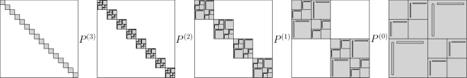
Figure 2: Illustration of the structure of the eigenmatrix $Q$, where $l_{\max}=4$ and each structured diagonal block (marked in gray) is for an intermediate eigenmatrix $\hat{Q}_{p}$ associated with a nonleaf node $p$.

Thus, $Q$ can be understood in terms of either (64) or the local eigenmatrices. Lemma 4.2 gives an efficient way to apply $Q$ or $Q^{T}$ to a vector, where the triangular FMM with local shifting is again used to multiply the intermediate eigenmatrices with vectors. Note that with a very similar procedure, a local eigenmatrix $Q_{i}$ or its transpose can be conveniently applied to a vector. Such an application process is used to multiply the local eigenmatrices $Q_{i}^{T}$ and $Q_{j}^{T}$ to $Z_{p}$ as in (9) so as to quickly form $\hat{Z}_{p}$ used in (61).

In addition, as mentioned in [35], each intermediate eigenmatrix $\hat{Q}_{i}$ has small off-diagonal numerical ranks. An off-diagonal numerical rank result given in [35] is in terms of entrywise approximations. The overall eigenmatrix $Q$ itself does not necessarily have a small off-diagonal numerical rank, so a remark in [35] is not precise. In fact, a precise off-diagonal numerical rank bound for $\hat{Q}_{i}$ in terms of singular value truncation can be shown based on the studies in [43]. Then, if the matrices $P^{(l)}$ are dropped from $Q$ in (64), the resulting matrix has small off-diagonal numerical ranks.

The main algorithms used in SuperDC are shown in the supplementary materials. When $A$ is given in terms of an HSS form with HSS rank $r$, the total complexity for computing the eigendecomposition (1) can be counted following [35, Section 3.1] and is $O(r^{2}n\log^{2}n)$. (There is an erratum for [35] in the flop count since $r$ in equation (3.1) of [35, Section 3.1] should be $r^{2}$.) Note that the use of all the new stability techniques here does not change the overall complexity. Every local eigenmatrix $\hat{Q}_{i}$ is represented by a sequence of $r$ Cauchy-like matrices like in (56). Each such a Cauchy-like matrix is stored with the aid of five vectors like in (60). The storage for $Q$ is then $O(rn\log n)$ and the cost to apply $Q$ or $Q^{T}$ to a vector is $O(rn\log n)$ as in [35].

5 Numerical experiments

We then make a comprehensive test of the SuperDC eigensolver in terms of different types of matrices and demonstrate its efficiency and accuracy. SuperDC has been implemented in Matlab (available from https://www.math.purdue.edu/~xiaj) and is compared with the highly optimized Matlab eig function for computing the eigendecomposition. We also show the significance of our stability techniques. The accuracy measurements follow those in [21, 35]:

$$\hskip 85.35826pt\gamma =\max\limits_{1\leq k\leq n}\frac{\|A\mathbf{q_{k}}-\lambda_{k}\mathbf{q}_{k}\|_{2}}{n\|A\|_{2}}$$ (residual),

$$\delta =\frac{\sqrt{\sum_{k=1}^{n}(\lambda_{k}^{\ast}-\lambda_{k})^{2}}}{n\sqrt{\sum_{k=1}^{n}(\lambda_{k}^{\ast})^{2}}}$$ (relative error),

$$\theta =\max\limits_{1\leq k\leq n}\frac{\|Q^{T}{\mathbf{q}}_{k}-\mathbf{e}_{k}\|_{2}}{n}$$ (loss of orthogonality),

where $\lambda_{k}^{\ast}$’s are eigenvalues from eig and are considered as the exact results. The triangular FMM routine is developed based on a code used in [8]. The accuracy of each triangular FMM is set to reach full machine precision so that it does not interfere with the orthogonality of the eigenvectors. The tests are performed with four 2.60GHz cores and 80GB memory on a node at a cluster of Purdue RCAC. The usage of 80GB memory is just to accommodate the need of eig for larger matrices.

Example 5.1.

We first consider a symmetric tridiagonal matrix $A$. The classical divide-and-conquer eigensolver does not need tridiagonal reduction and can be directly applied to $A$ with $O(n^{3})$ cost and $O(n^{2})$ storage. For our SuperDC eigensolver, the HSS representation of $A$ can be explicitly written out without any extra cost and its HSS rank is $r=2$ [40]. (The HSS structure does not rely on the actual nonzero entries, which are $3$ on the main diagonal and $-1$ on the first superdiagonal and subdiagonal. Other numbers such as random ones are also tested with similar performance observed.) The size $n$ of $A$ in the test ranges from $8192$ to $262,144$. In the HSS form, the leaf-level diagonal block size is $2048$. We use $\tau=10^{-10}$ in the deflation criterion (Remark 4.1).

The timing (in seconds) of SuperDC and eig are reported in Figure 3(a). The storage for the eigenmatrix $Q$ (in terms of nonzeros) is given in Figure 3(b). The costs of SuperDC in terms of the eigendecomposition flops and the flops to apply $Q$ to a vector are given in Figure 3(c). SuperDC achieves nearly linear complexity in all the aspects (timing, flops, and storage), while eig exhibits a cubic trend in timing and an obvious quadratic storage (which is just $n^{2}$ for storing the dense $Q$). In fact, the flop count of SuperDC in Figure 3(c) shows a pattern even slightly better than $O(n\log^{2}n)$. The timing is slightly off, likely due to the implementation.

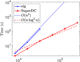
(a) Eigendecomposition timing

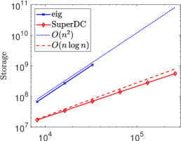
(b) Storage

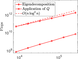
(c) Flops of SuperDC

Figure 3: Example 1. Timing and storage of SuperDC and eig and flops of SuperDC.

SuperDC is faster than eig for all the tested sizes. With $n=32,768$, SuperDC is already over $6$ times faster than eig and takes only about $6\%$ of the memory. (We also tested $n$ as small as $4096$ and SuperDC already has lower storage and has comparable timing.) Note that eig runs out of memory for larger $n$ due to the dense eigenmatrix, while SuperDC takes much less memory and can reach much larger $n$. For SuperDC, the timing is mostly for the conquering stage. For example, for $n=262,144$, SuperDC takes $383.4$ seconds, where the dividing stage needs just $16.1$ seconds. This also confirms that our strategy in Section 3 for reducing the ranks of low-rank updates is important since it directly saves the cost in the conquering stage.

Table 1 shows the accuracy of SuperDC. The eigenvalues are computed accurately and the loss of orthogonality $\theta$ is around machine precision.

Table 1: Example 5.1. Accuracy of SuperDC, where some errors ($\delta$) are not reported since eig runs out of memory, and the case $n=262,144$ is not shown since it takes too long to compute $\gamma$ and $\theta$.

$n$	$8,192$	$16,384$	$32,768$	$65,536$	$131,072$
$\gamma$	$1.9e-16$	$8.8e-16$	$5.2e-16$	$3.0e-16$	$1.5e-16$
$\delta$	$1.6e-18$	$8.0e-18$	$2.9e-18$
$\theta$	$6.4e-16$	$2.3e-16$	$1.9e-16$	$2.1e-16$	$1.8e-16$

Example 5.2.

Next, we consider a symmetric matrix $A$ which is sparse and nearly banded. That is, $A$ has a banded form with half bandwidth $5$ together with some nonzero entries away from the band. The HSS form for $A$ can be explicitly written out and has HSS rank $10$. The main diagonal entries are equal to $3$ and the other entries in the band are equal to $-1$. The nonzero entries away from the band are introduced by modifying some HSS generators for the banded matrix constructed with the method in [40]. In the HSS form, the leaf-level diagonal block size is $2048$. We use $\tau=10^{-10}$ in the deflation criterion (Remark 4.1).

The entries away from the band break the banded structure of $A$. The efficiency benefit of SuperDC becomes even more significant, as shown in Figure 4. At $n=32,678$, SuperDC is already about $11$ times faster than eig and takes only about $7\%$ of the memory. Again, eig runs out of memory when $n$ increases further, but SuperDC works for much larger $n$ and demonstrates nearly linear complexity in the all aspects.

Table 2 shows the accuracy of SuperDC. Similarly, high accuracies are achieved.

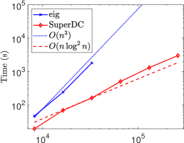
(a) Eigendecomposition timing

(b) Storage

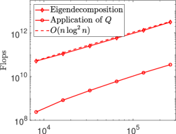
(c) Flops of SuperDC

Figure 4: Example 5.2. Timing and storage of SuperDC and eig and flops of SuperDC.

Table 2: Example 5.2. Accuracy of SuperDC, where some errors ($\delta$) are not reported since eig runs out of memory, and the case $n=262,144$ is not shown since it takes too long to compute $\gamma$ and $\theta$.

$n$	$8,192$	$16,384$	$32,768$	$65,536$	$131,072$
$\gamma$	$6.5e-15$	$6.8e-15$	$1.2e-14$	$1.1e-15$	$1.1e-14$
$\delta$	$1.4e-17$	$6.5e-18$	$8.1e-17$
$\theta$	$1.8e-15$	$2.8e-15$	$2.4e-15$	$4.8e-15$	$2.3e-15$

In addition, in order to demonstrate the importance of our local shifting strategy, we have tested the eigensolver with triangular FMM accelerations applied to the original secular equation instead of the shifted one. Other than the case with $n=8192$, Matlab returns NaN (not-a-number) for all the larger matrix sizes due to cancellations. This confirms the risk of directly applying FMM accelerations to the usual secular equation like in [35].

Example 5.3.

Then consider a dense symmetric matrix $A$ which is a Toeplitz matrix with its first row $\boldsymbol{\xi}=\begin{pmatrix}\xi_{1}&\cdots&\xi_{n}\end{pmatrix}$ given by

$$\xi_{1}=2\alpha,\quad\xi_{j}=\frac{\sin(2\alpha(j-1)\pi)}{(j-1)\pi},\ j=2,3,\ldots,n,$$

where $0<\alpha<1/2$. This is the so-called Prolate matrix that appears frequently in signal processing. It is known to be extremely ill-conditioned and has special spectral properties (see, e.g., [34]). In this example, we set $\alpha=\frac{1}{4}$. It is known that any Toeplitz matrix can be converted into a Cauchy-like matrix $\mathcal{C}$ which has small off-diagonal numerical ranks [12, 28, 35]. That is, $\mathcal{C}=\mathcal{F}A\mathcal{F}^{\ast}$, where $\mathcal{F}$ is the normalized inverse DFT matrix. The eigendecomposition of $A$ can then be done via that of $\mathcal{C}$. An HSS approximation to $\mathcal{C}$ may be quickly constructed based on randomized methods in [26, 27, 42, 46] coupled with fast Toeplitz matrix-vector multiplications. The cost is nearly linear in $n$. Here, we use a tolerance $10^{-10}$ in relevant compression steps, which is same as the deflation tolerance $\tau$. In the HSS form, the leaf-level diagonal block size is $2048$. SuperDC is applied to the resulting HSS form and compared with eig applied to $A$. The size $n$ ranges from $4096$ to $65,536$.

In Figure 5, the timing, storage, and flops are shown and are consistent with the complexity estimates. The eigendecomposition with SuperDC shows a dramatic efficiency advantage over eig. At $n=32,768$, eig takes $1526.2$ seconds, while SuperDC only needs $11.2$ seconds, which is a difference of about $136$ times. Also, the memory saving is about $15$ times.

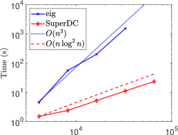
(a) Eigendecomposition timing

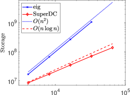
(b) Storage

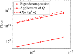
(c) Flops of SuperDC

Figure 5: Example 5.3. Timing and storage of SuperDC and eig and flops of SuperDC.

One thing we want to point out is that SuperDC has the theoretical complexity $O(r^{2}n\log^{2}n)$, which may overestimate the actual cost. For example, here $r$ is typically known to be $O(\log n)$. (This bound is based on entrywise approximations, although a precise numerical rank may be slightly higher [43].) One reason for the overestimate is that the flop count does not take into consideration a levelwise rank pattern in [41]. Another reason is our flexible deflation strategy in Remark 4.1. The matrices actually have highly clustered eigenvalues, which further leads to high efficiency gain.

Despite the clustered eigenvalues, SuperDC still computes the eigendecomposition accurately. See Table 3.

Table 3: Example 5.3. Accuracy of SuperDC, where the error ($\delta$) for $n=65,536$ is not reported since eig runs out of memory.

$n$	$4,096$	$8,192$	$16,384$	$32,768$	$65,536$
$\gamma$	$1.5e-16$	$6.7e-14$	$2.3e-17$	$1.3e-17$	$3.3e-18$
$\delta$	$7.8e-15$	$1.7e-15$	$2.3e-14$	$3.7e-14$
$\theta$	$3.4e-17$	$9.3e-17$	$4.6e-17$	$2.3e-17$	$1.2e-17$

Example 5.4.

Our last example is a discretized kernel matrix $A$ in [10] which is the evaluation of the function $\sqrt{|s-t|}$ at the Chebyshev points $\cos(\frac{2i-1}{2n}\pi),i=1,2,\ldots,n$. The HSS construction may be based on direct off-diagonal compression or efficient analytical methods like in [47]. We use an existing routine based on the former one for simplicity. To show the flexibility of accuracy controls, we aim for moderate accuracy in this test by using a compression tolerance $10^{-6}$ in the HSS construction, which is same as the deflation tolerance $\tau$.

For this example, we can observe similar complexity results as in the previous examples. See Figure 6, where we still set the leaf-level diagonal block size to be $2048$ in the HSS approximations. With the larger tolerance than in the previous examples, we still achieve reasonable eigenvalue errors and residuals as in Table 4. The loss of orthogonality is still close to machine precision. Thus for the remaining discussions, we focus on some stability advantages of SuperDC.

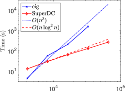
(a) Eigendecomposition timing

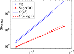
(b) Storage

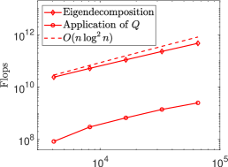
(c) Flops of SuperDC

Figure 6: Example 5.4. Timing and storage of SuperDC and eig and flops of SuperDC.

Table 4: Example 5.4. Accuracy of SuperDC, where the error ($\delta$) for $n=65,536$ is not reported since eig runs out of memory.

$n$	$4,096$	$8,192$	$16,384$	$32,768$	$65,536$
$\gamma$	$1.2e-10$	$9.9e-11$	$1.7e-10$	$1.5e-10$	$9.1e-11$
$\delta$	$1.6e-11$	$2.5e-11$	$2.1e-11$	$1.1e-11$
$\theta$	$1.6e-15$	$8.0e-15$	$2.7e-15$	$3.4e-15$	$3.4e-15$

Earlier in Example 5.2, it is shown that local shifting helps avoid cancellations so that FMM accelerations can be applied reliably. In fact, even if there is no cancellation in the original secular equation solution, our local shifting strategy (for triangular FMM-accelerated solution of the shifted secular equation) can further greatly benefit the convergence. To illustrate this, we perform the following count. Suppose $r$ secular equations are solved due to $r$ rank-$1$ updates associated with the root node of the HSS tree $\mathcal{T}$. Let $\mu_{j}$ be the percentage of eigenvalues that have not converged after $5$ iterations during modified Newton’s solution of the secular equation associated with the $j$th rank-one update, and let $\mu=\max_{1\leq j\leq r}\mu_{j}$. Table 5 reports this maximum percentage $\mu$ with varying $n$. With local shifting, a vast majority of those eigenvalues (about $99\%$ or more) converges within $5$ iterations. This is significantly better than the case without local shifting (i.e., when the original secular equation is solved with FMM accelerations).

Table 5: Maximum percentage ($\mu$) of eigenvalues not converged within $5$ iterations for solving the $r$ secular equations associated with $\operatorname{root}(\mathcal{T})$.

$n$	$4,096$	$8,192$	$16,384$	$32,768$	$65,536$
With local shifting	$1.03\%$	$0.75\%$	$0.91\%$	$0.89\%$	$0.84\%$
Without local shifting	$69.1\%$	$65.2\%$	$65.0\%$	$60.1\%$	$53.7\%$

We would then also like to demonstrate the advantage of our stable dividing strategy in Section 3 as compared with the original one in [35]. Following Propositions 3.1 and 3.3, we show the norm growth of the $B,D$ generators after the dividing stage. For the initial $B,D$ generators of the original HSS form, let $\tilde{B},\tilde{D}$ denote the updated generators after the entire dividing stage is finished. Then let

$$\rho_{B}=\max\limits_{i<\operatorname{root}(\mathcal{T})}\!\|B_{i}\|_{2},\quad\rho_{D}=\max\limits_{i\text{: leaf}}\|D_{i}\|_{2},\quad\rho_{\tilde{B}}=\max\limits_{i<\operatorname{root}(\mathcal{T})}\!\|\tilde{B}_{i}\|_{2},\quad\rho_{\tilde{D}}=\max\limits_{i\text{: leaf}}\|\tilde{D}_{i}\|_{2}.$$

In order to better show the norm growth after multilevel dividing, we set the leaf-level diagonal block size to be $256$ here so as to have more levels. For each $n$, Table 6 shows the number of levels in the HSS approximation. When $n$ increases, the HSS tree $\mathcal{T}$ grows deeper. Table 6 shows that $\|A\|_{2}$ and $\rho(B)$ grow roughly linearly with $n$. However, $\rho_{\tilde{B}}$ and $\rho_{\tilde{D}}$ grow exponentially with the original dividing stage in [35], as predicted by Proposition 3.1. This poses a stability risk. When $n$ grows beyond a certain size, overflow happens. (Note that $\rho_{\tilde{D}}$ has a larger magnitude than $\rho_{\tilde{B}}$, which is consistent with Proposition 3.1.) In contrast, the growth of $\rho_{\tilde{D}}$ and $\rho_{\tilde{B}}$ with our new dividing strategy is much slower and roughly follows the growth pattern of $\rho(B)$, as predicted by Proposition 3.3. Accordingly, our algorithm can handle much larger $n$ much more reliably.

Table 6: Example 5.4. Norm growth of the $D,B$ generators after the dividing stage, where $\infty$ means overflow.

$n$		$4,096$	$8,192$	$16,384$	$32,768$	$65,536$
Number of levels		$5$	$6$	$7$	$8$	$9$
$\|A\|_{2}$		$3.4e03$	$6.8e03$	$1.4e04$	$2.7e04$	$5.4e04$
Initial	$\rho_{B}$	$2.3e03$	$4.6e03$	$9.2e03$	$1.8e04$	$3.7e04$
	$\rho_{D}$	$6.1e01$	$4.3e01$	$3.1e01$	$2.2e01$	$1.5e01$
After the original	$\rho_{\tilde{B}}$	$5.5e24$	$9.9e53$	$2.1e117$	$4.2e253$	$\infty$
dividing strategy	$\rho_{\tilde{D}}$	$3.0e49$	$9.9e107$	$4.5e234$	$\infty$	$\infty$
After the new	$\rho_{\tilde{B}}$	$2.3e03$	$4.6e03$	$9.2e03$	$2.1e04$	$5.5e04$
dividing strategy	$\rho_{\tilde{D}}$	$4.7e03$	$1.2e04$	$3.4e04$	$8.6e04$	$2.4e05$

6 Conclusions

In this work, we have designed the SuperDC eigensolver that is both superfast and stable. It significantly improves the original divide-and-conquer algorithm in [35] in both the stability and the algorithm design. A series of stability techniques is built into the different stages of the algorithm. In particular, we avoid an exponential norm growth risk in the dividing stage via a balancing strategy and are further able to combine FMM accelerations with several key stability safeguards that have been used in practical divide-and-conquer algorithms. We also give a variety of algorithm designs and structure studies that have been missing or unclear in [35]. The comprehensive numerical tests confirm the nearly linear complexity and much higher efficiency than the Matlab eig function for the eigendecomposition of different types of HSS matrices. Nice accuracy and eigenvector orthogonality have been observed. Comparisons also illustrate the benefits of our stability techniques.

The SuperDC eigensolver makes it feasible to use full eigendecompositions to solve various challenging numerical problems as mentioned at the beginning of the paper. A list of applications is expected to be included in [36]. In addition, we expect that the novel local shifting strategy and triangular FMM accelerations are also useful for other FMM-related matrix computations when stability and accuracy are crucial. In our future work, we plan to provide a high-performance parallel implementation, which will extend the applicability of the algorithm to large-scale numerical computations.

Supplementary materialsXiaofeng Ou and Jianlin Xia

SUPPLEMENTARY MATERIALS:
LIST OF MAJOR ALGORITHMS

Title of paper: SuperDC: Stable superfast divide-and-conquer eigenvalue decomposition
Authors: Xiaofeng Ou and Jianlin Xia

These supplementary materials are pseudocodes that can help better understand the major algorithms in the paper.

• Algorithm 1: the HSS dividing stage.

• Algorithm 2: solving the secular equation for the eigenvalues with triangular FMM accelerations and local shifting.

• Algorithm 3: the conquering stage for producing the eigendecomposition.

• Algorithm 4: application of the a local eigenmatrix $Q_{i}$ or its transpose to a vector. This is used in Algorithm 3 and also can be used to apply the global eigenmatrix $Q$ or its transpose to a vector when $i=\operatorname{root}(\mathcal{T})$.

For notational convenience, we use $r$ to represent the column sizes of all $Z_{i}$ matrices in the pseudocodes. $\mathcal{T}_{i}$ is also used to denote the subtree of $\mathcal{T}$ rooted at node $i\in\mathcal{T}$. $Z(:,j)$ means the $j$-th column of $Z$.

The following utility routines are used in the algorithms. To save space, we are not showing pseudocodes for these routines.

• $\mathsf{updhss}(D_{i},U_{i},H)$: for an HSS block $D_{i}$ corresponding to the subtree $\mathcal{T}_{i}$, update its $D,B$ generators to get those of $D_{i}-U_{i}HU_{i}^{T}$ using Lemma 2.1.

• $\mathsf{trifmm}(\mathbf{d},\mathbf{x},\boldsymbol{y},\mathbf{w},\kappa)$: compute a matrix-vector product $K\mathbf{w}$ with the triangular FMM and local shifting as in Sections 4.1.2 and 4.2.2, where $K=(\kappa(d_{i},x_{j}))_{d_{i}\in\mathbf{d},x_{j}\in\mathbf{x}}$ is a kernel matrix and $\boldsymbol{y}$ is the gap vector (for accurately evaluating $\mathbf{x}-\mathbf{d}$). Note that the triangular FMM is used to multiply the lower triangular part of $K$ with $\mathbf{w}$ and the strictly upper triangular part of $K$ with $\mathbf{w}$ and the final result is the sum of the two products.

• $\mathsf{mnewton}(\boldsymbol{\psi},\boldsymbol{\phi},\boldsymbol{\psi}^{\prime},\boldsymbol{\phi}^{\prime})$: use the modified Newton’s method to compute corrections to the current approximate gap as in (47), where $\boldsymbol{\psi},\boldsymbol{\phi},\boldsymbol{\psi}^{\prime},\boldsymbol{\phi}^{\prime}$ look like (38) and (39).

• $\mathsf{iniguess}(\mathbf{d},\mathbf{w})$: compute the initial guess as in [22] for the solution of the secular equation (13).

• $\mathsf{deflate}(\mathbf{d},\mathbf{v},\tau)$: apply deflation with the criterion in Remark 4.1.

Algorithm 1 SuperDC dividing stage

1:procedure divide($\{D_{i}\}_{i\in\mathcal{T}},\{U_{i}\}_{i\in\mathcal{T}},\{R_{i}\}_{i\in\mathcal{T}},\{B_{i}\}_{i\in\mathcal{T}}$)

2:     for node $i=\text{root}(\mathcal{T}),\ldots,1$ do$\triangleright$ Dividing $D_{i}$ in a top-down traversal

3:         if $i$ is a non-leaf node then

4:              if $\operatorname{colsize}(B_{c_{1}})\leq\operatorname{rowsize}(B_{c_{1}})$ then$\triangleright$ $c_{1},c_{2}$: children of $i$

5:                  $D_{c_{1}}\leftarrow\mathsf{updhss}(D_{c_{1}},U_{c_{1}},\frac{1}{\|B_{c_{1}}\|_{2}}B_{c_{1}}B_{c_{1}}^{T})$$\triangleright$ Update generators of $D_{c_{1}}$
to get those of $D_{c_{1}}-\frac{1}{\|B_{c_{1}}\|_{2}}U_{c_{1}}B_{c_{1}}B_{c_{1}}^{T}U_{c_{1}}^{T}$ like in Lemma 2.1

6:                  $D_{c_{2}}\leftarrow\mathsf{updhss}(D_{c_{2}},U_{c_{2}},\|B_{c_{1}}\|_{2}I)$$\triangleright$ Update generators of $D_{c_{2}}$
to get those of $D_{c_{2}}-\|B_{c_{1}}\|_{2}U_{c_{2}}U_{c_{2}}^{T}$ like in Lemma 2.1

7:              else

8:                  $D_{c_{1}}\leftarrow\mathsf{updhss}(D_{c_{1}},U_{c_{1}},\|B_{c_{1}}\|_{2}I)$$\triangleright$ Update generators of $D_{c_{1}}$
to get those of $D_{c_{1}}-\|B_{c_{1}}\|_{2}U_{c_{1}}U_{c_{1}}^{T}$ like in Lemma 2.1

9:                  $D_{c_{2}}\leftarrow\mathsf{updhss}(D_{c_{2}},U_{c_{2}},\frac{1}{\|B_{c_{1}}\|_{2}}B_{c_{1}}^{T}B_{c_{1}})$$\triangleright$ Update generators of $D_{c_{2}}$
to get those of $D_{c_{2}}-\frac{1}{\|B_{c_{1}}\|_{2}}U_{c_{2}}B_{c_{1}}^{T}B_{c_{1}}U_{c_{2}}^{T}$ like in Lemma 2.1

10:              end if

11:         end if

12:     end for

13:     for node $i=1,\ldots,\text{root}(\mathcal{T})$ do$\triangleright$ Form $Z_{i}$ in a bottom-up traversal

14:         if $i$ is a non-leaf node then

15:              if $\operatorname{colsize}(B_{c_{1}})\leq\operatorname{rowsize}(B_{c_{1}})$ then$\triangleright$ $c_{1},c_{2}$: children of $i$

16:                  $Z_{i}\leftarrow\begin{pmatrix}\frac{1}{\sqrt{\|B_{c_{1}}\|_{2}}}U_{c_{1}}B_{c_{1}}\\ \sqrt{\|B_{c_{1}}\|_{2}}U_{c_{2}}\end{pmatrix}$ $\triangleright$ Local update $Z$ matrix like in (27)

17:              else

18:                  $Z_{i}\leftarrow\begin{pmatrix}\sqrt{\|B_{c_{1}}\|_{2}}U_{c_{1}}\\ \frac{1}{\sqrt{\|B_{c_{1}}\|_{2}}}U_{c_{2}}B_{c_{1}}^{T}\end{pmatrix}$ $\triangleright$ Local update $Z$ matrix like in (30)

19:              end if

20:              if $i\neq\text{root}(\mathcal{T})$ then

21:                  $U_{i}\leftarrow\begin{pmatrix}U_{c_{1}}R_{c_{1}}\\ U_{c_{2}}R_{c_{2}}\end{pmatrix}$ $\triangleright$ Assemble $U_{i}$ for parent node of $i$

22:              end if

23:         end if

24:     end for

25:     return updated generators $\{D_{i}\}_{i\in\mathcal{T}},\{B_{i}\}_{i\in\mathcal{T}},\{Z_{i}\}_{i\in\mathcal{T}}$

26:end procedure

Algorithm 2 Secular equation solution for eigenvalues (of $\operatorname{diag}(\mathbf{d})+\mathbf{v}\mathbf{v}^{T}$)

1:procedure secular($\mathbf{d},\mathbf{v}$) $\triangleright$ Eigenvalue solution via the solution of the shifted secular equation (43)

2:     $\mathbf{w\leftarrow v\odot v}$

3:     $\mathbf{y}^{(0)}\leftarrow\mathsf{iniguess}(\mathbf{d},\mathbf{w})$$\triangleright$ Computation of the initial guess as in [22]

4:     $\boldsymbol{x}^{(0)}\leftarrow\mathbf{y}^{(0)}+\mathbf{d}$

5:     for $j=0,1,\ldots$ do

6:         $[\boldsymbol{\psi},\boldsymbol{\phi}]\leftarrow\mathsf{trifmm}(\mathbf{d},\mathbf{x}^{(j)},\boldsymbol{y}^{(j)},\mathbf{w},\frac{1}{s-t})$$\triangleright$ Computation of $\boldsymbol{\psi},\boldsymbol{\phi}$ in (38)

7:         $[\boldsymbol{\psi}^{\prime},\boldsymbol{\phi}^{\prime}]\leftarrow\mathsf{trifmm}(\mathbf{d},\mathbf{x}^{(j)},\boldsymbol{y}^{(j)},\mathbf{w},\frac{1}{(s-t)^{2}})$$\triangleright$ Computation of $\boldsymbol{\psi}^{\prime},\boldsymbol{\phi}^{\prime}$ in (39)

8:         $\mathbf{f}\leftarrow\mathbf{e}+\boldsymbol{\psi}+\boldsymbol{\phi}$

9:         if $|\mathbf{f}|<cn(\mathbf{e}+|\boldsymbol{\psi}|+|\boldsymbol{\phi}|)\epsilon$ then $\triangleright$ Stopping criterion

10:              break

11:         end if

12:         $\Delta\mathbf{x}^{(j)}\leftarrow\mathsf{mnewton}(\boldsymbol{\psi},\boldsymbol{\phi},\boldsymbol{\psi}^{\prime},\boldsymbol{\phi}^{\prime})$ $\triangleright$ Computation of root update with modified Newton’s method

13:         $\boldsymbol{y}^{(j+1)}\leftarrow\boldsymbol{y}^{(j)}+\Delta\mathbf{x}^{(j)}$$\triangleright$ Updated gap approximation as in (47)

14:         $\mathbf{x}^{(j+1)}\leftarrow\boldsymbol{y}^{(j+1)}+\mathbf{d}$$\triangleright$ Updated eigenvalue approximation

15:     end for

16:     $\boldsymbol{\lambda}\leftarrow\mathbf{x}^{(j)}$, $\boldsymbol{\eta}\leftarrow\boldsymbol{y}^{(j)}$$\triangleright$ Eigenvalue and gap upon convergence

17:     return $\boldsymbol{\lambda},\boldsymbol{\eta}$

18:end procedure

Algorithm 3 SuperDC conquering stage

1:procedure conquer($\{D_{i}\}_{i\in\mathcal{T}},\{U_{i}\}_{i\in\mathcal{T}},\{R_{i}\}_{i\in\mathcal{T}},\{B_{i}\}_{i\in\mathcal{T}},\{Z_{i}\}_{i\in\mathcal{T}},\tau$) $\triangleright$ The $D_{i},B_{i}$ generators have been updated in the dividing stage

2:     for node $i=1,\ldots,\operatorname{root}(\mathcal{T})$ do$\triangleright$ Conquering in a postordered traversal

3:         if $i$ is a leaf node then$\triangleright$ Leaf-level eigendecomposition

4:              $(\boldsymbol{\lambda}_{i},\hat{Q}_{i})\leftarrow\mathsf{eig}(D_{i})$$\triangleright$ Via Matlab eig function

5:         else

6:              $\begin{pmatrix}{Z_{i,1}}\\ {Z_{i,2}}\end{pmatrix}\leftarrow Z_{i}$$\triangleright$ Partitioning following the sizes of $D_{c_{1}}$ and $D_{c_{2}}$

7:              ${Z_{i,1}}\leftarrow\mathsf{superdcmv}(Q_{c_{1}},{Z_{i,1}},1)$$\triangleright$ $Q_{c_{1}}^{T}{Z_{i,1}}$

8:              ${Z_{i,2}}\leftarrow\mathsf{superdcmv}(Q_{c_{2}},{Z_{i,2}},1)$$\triangleright$ $Q_{c_{2}}^{T}{Z_{i,2}}$

9:              $Z_{i}\leftarrow\begin{pmatrix}{Z_{i,1}}\\ {Z_{i,2}}\end{pmatrix}$$\triangleright$ $\hat{Z}_{i}$ like in (9)

10:              $[\boldsymbol{\lambda}_{i}^{(0)},P_{i}]\leftarrow\mathsf{sort}(\boldsymbol{\lambda}_{c_{1}},\boldsymbol{\lambda}_{c_{2}})$$\triangleright$ Ordering of all the diagonal entries
of $\boldsymbol{\lambda}_{c_{1}},\boldsymbol{\lambda}_{c_{2}}$ together, with $P_{i}$ the permutation matrix

11:              for $j=1,2\ldots,r$ do$\triangleright$ $r=\operatorname{colsize}(Z_{i})$

12:                  $[\mathbf{d}_{i}^{(j)},Z_{i}(:,j)]\leftarrow\mathsf{deflate}(\boldsymbol{\lambda}_{i}^{(j-1)},Z_{i}(:,j),\tau)$$\triangleright$ Deflation (Remark 4.1)

13:                  $[\boldsymbol{\lambda}_{i}^{(j)},\boldsymbol{\eta}_{i}^{(j)}]\leftarrow\mathsf{secular}(\mathbf{d}_{i}^{(j)},Z_{i}(:,j))$$\triangleright$ Secular equation solution

14:                  $\mathbf{v}_{1}\leftarrow\mathsf{trifmm}(\mathbf{d}_{i}^{(j)},\boldsymbol{\lambda}_{i}^{(j)},\boldsymbol{\eta}_{i}^{(j)},\mathbf{e},\log|s-t|)$$\triangleright$ $G_{1}\mathbf{e}$ as needed in (55)

15:                  $\mathbf{v}_{2}\leftarrow\mathsf{trifmm}(\mathbf{d}_{i}^{(j)},\mathbf{d}_{i}^{(j)},\mathbf{0},\mathbf{e},\log|s-t|)$$\triangleright$ $G_{2}\mathbf{e}$ as needed in (55)

16:                  $\mathbf{\hat{v}}_{i}^{(j)}\leftarrow\exp{(}\frac{{\mathbf{v}_{1}-\mathbf{v}_{2}}}{2}{)}$$\triangleright$ Löwner’s formula for $\mathbf{\hat{v}}$ as in (53)–(55)

17:                  $\mathbf{b}_{i}^{(j)}\leftarrow$ $(\mathsf{trifmm}(\mathbf{d}_{i}^{(j)},\boldsymbol{\lambda}_{i}^{(j)},\boldsymbol{\eta}_{i}^{(j)},\mathbf{\hat{v}}_{i}^{(j)}\odot\mathbf{\hat{v}}_{i}^{(j)},\frac{1}{(s-t)^{2}}))^{-1/2}$ $\triangleright$ Normalization factor as in (57)

18:                  $\hat{Q}_{i}^{(j)}\leftarrow\{\mathbf{\hat{v}}_{i}^{(j)},\mathbf{b}_{i}^{(j)},\mathbf{d}_{i}^{(j)},\boldsymbol{\lambda}_{i}^{(j)},\boldsymbol{\eta}_{i}^{(j)}\}$$\triangleright$ Cauchy-like structured
representation of the local eigenmatrix as in (56)

19:                  for $k=j+1,j+2,\ldots,r$ do$\triangleright$ Multiplication of $(\hat{Q}_{i}^{(j)})^{T}$
to the remaining columns of $Z_{i}$ via the steps as in (59)

20:                       $Z_{i}(:,k)\leftarrow\mathbf{\hat{v}}_{i}^{(j)}\odot Z_{i}(:,k)$

21:                       $Z_{i}(:,k)\leftarrow-\mathsf{trifmm}(\boldsymbol{\lambda}_{i}^{(j)},\mathbf{d}_{i}^{(j)},\boldsymbol{\eta}_{i}^{(j)},Z_{i}(:,k),\frac{1}{s-t})$ $\triangleright$ The negative sign and the switch of
$\boldsymbol{\lambda}_{i}^{(j)}$ and $\mathbf{d}_{i}^{(j)}$ are due to the transpose

22:                       $Z_{i}(:,k)\leftarrow\mathbf{b}_{i}^{(j)}\odot Z_{i}(:,k)$

23:                  end for

24:              end for

25:              $\boldsymbol{\lambda}_{i}\leftarrow\boldsymbol{\lambda}_{i}^{(r)}$$\triangleright$ Local eigenvalues associated with node $i$

26:         end if

27:     end for

28:     $\boldsymbol{\lambda}\leftarrow\boldsymbol{\lambda}_{\operatorname{root}(\mathcal{T})}$, $Q\leftarrow\{\{\hat{Q}_{i}^{(j)}\}_{j=1}^{r},P_{i}\}_{i\in\mathcal{T}}$$\triangleright$ Final eigenvalues
and eigenmatrix $Q$ in (64), with $\hat{Q}_{i}$ in (63) given by $\prod_{j=1}^{r}\hat{Q}_{i}^{(j)}$

29:     return $\boldsymbol{\lambda},Q$

30:end procedure

Algorithm 4 SuperDC eigenmatrix-vector multiplication

1:procedure superdcmv($Q_{i},\mathbf{x},\text{transpose}$)$\triangleright$ Application of a local eigenmatrix $Q_{i}$
or its transpose to a vector $\mathbf{x}$, depending on whether ‘transpose’ is $0$ or $1$

2:     $i_{1}\leftarrow$ smallest descendant of $i$

3:     if $\text{transpose}=0$ then$\triangleright$ $\mathbf{y}=Q_{i}\mathbf{x}$

4:         $\mathbf{y}_{i}\leftarrow\mathbf{x}$

5:         for $k=i,i-1,\ldots,i_{1}$ do$\triangleright$ Reverse postordered traversal of $\mathcal{T}_{i}$

6:              if $k$ is leaf then

7:                  $\mathbf{y}_{k}\leftarrow Q_{k}\mathbf{y}_{k}$$\triangleright$ Dense ${Q}_{k}$ at the leaf level

8:              else

9:                  for $j=r,r-1,\ldots,1$ do$\triangleright$ Multiplication of $\hat{Q}_{k}^{(j)}$
via the steps like in (59)

10:                       $\mathbf{y}_{k}\leftarrow\mathbf{b}_{k}^{(j)}\odot\mathbf{y}_{k}$

11:                       $\mathbf{y}_{k}\leftarrow\mathsf{trifmm}(\mathbf{d}_{k}^{(j)},\boldsymbol{\lambda}_{k}^{(j)},\boldsymbol{\eta}_{k}^{(j)},\mathbf{y}_{k},\frac{1}{s-t})$

12:                       $\mathbf{y}_{k}\leftarrow\mathbf{\hat{v}}_{k}^{(j)}\odot\mathbf{y}_{k}$

13:                  end for

14:                  $\mathbf{y}_{k}\leftarrow P_{k}^{T}\mathbf{y}_{k}$$\triangleright$ Permutation like in (62)

15:                  $\begin{pmatrix}\mathbf{y}_{c_{1}}\\ \mathbf{y}{{}_{c_{2}}}\end{pmatrix}\leftarrow\mathbf{y}_{k}$$\triangleright$ Partitioning following the sizes of $Q_{c_{1}},Q_{c_{2}}$,
with $c_{1},c_{2}$ the children of $k$

16:              end if

17:         end for

18:     else$\triangleright$ $\mathbf{y}=Q_{i}^{T}\mathbf{x}$

19:         Partition $\mathbf{x}$ into $\mathbf{x}_{k}$ pieces following the leaf-level $Q_{k}$ sizes

20:         for $k=i_{1},i_{1}+1,\ldots,i$ do$\triangleright$ Postordered traversal of $\mathcal{T}_{i}$

21:              if $k$ is leaf then

22:                  $\mathbf{y}_{k}\leftarrow Q_{k}^{T}\mathbf{x}_{k}$$\triangleright$ Dense ${Q}_{k}$ at the leaf level

23:              else

24:                  $\mathbf{y}_{k}\leftarrow\begin{pmatrix}\mathbf{y}_{c_{1}}\\ \mathbf{y}{{}_{c_{2}}}\end{pmatrix}$$\triangleright$ $c_{1},c_{2}$: children of $k$

25:                  $\mathbf{y}_{k}\leftarrow P_{k}\mathbf{y}_{k}$$\triangleright$ Permutation like in (62)

26:                  for $j=1,2,\ldots,r$ do$\triangleright$ Multiplication of $(\hat{Q}_{k}^{(j)})^{T}$
via the steps like in (59)

27:                       $\mathbf{y}_{k}\leftarrow\mathbf{\hat{v}}_{k}^{(j)}\odot\mathbf{y}_{k}$

28:                       $\mathbf{y}_{k}\leftarrow-\mathsf{trifmm}(\boldsymbol{\lambda}_{k}^{(j)},\mathbf{d}_{k}^{(j)},\boldsymbol{\eta}_{k}^{(j)},\mathbf{y}_{k},\frac{1}{s-t})$$\triangleright$ The negative sign
and the switch of $\boldsymbol{\lambda}_{k}^{(j)}$ and $\mathbf{d}_{k}^{(j)}$ are due to the transpose

29:                       $\mathbf{y}_{k}\leftarrow\mathbf{b}_{k}^{(j)}\odot\mathbf{y}_{k}$

30:                  end for

31:              end if

32:         end for

33:     end if

34:     return $\mathbf{y}$

35:end procedure

References

- [1] S. Ambikasaran and E. Darve, An fast direct solver for partial hierarchically semi-separable matrices, J. Sci. Comput., 57 (2013), pp. 477–501.
- [2] P. Amestoy, C. Ashcraft, O. Boiteau, A. Buttari, J.-Y. L’Excellent, and C. Weisbecker, Improving multifrontal methods by means of block low-rank representations, SIAM J. Sci. Comp., 37 (2015), pp. A1451–A1474.
- [3] E. Anderson, Z. Bai, C. Bischof, S. Blackford, J. Demmel, J. Dongarra, J. Du Croz, A. Greenbaum, S. Hammarling, A. McKenney, and D. Sorensen, LAPACK Users’ Guide, SIAM, Philadelphia, PA, third ed., 1999.
- [4] P. Benner and T. Mach, Computing all or some eigenvalues of symmetric -matrices, SIAM J. Sci. Comput., 34 (2012), pp. A485–A496.
- [5] D. A. Bini, L. Gemignani, and V. Y. Pan, Fast and stable QR eigenvalue algorithms for generalized companion matrices and secular equations, Numer. Math., 100 (2005), pp. 373–408.
- [6] D. Bini and V. Y. Pan, Parallel complexity of tridiagonal symmetric eigenvalue problem, in Proceedings of the 2nd Annual ACM-SIAM Symposium on Discrete Algorithms, SIAM, Philadelphia, 1991 pp. 384–393.
- [7] J. R. Bunch, C. P. Nielsen, and D. C. Sorensen, Rank-one modification of the symmetric eigenproblem, Numer. Math., 31 (1978), pp. 31–48.
- [8] D. Cai and J. Xia, A stable matrix version of the fast multipole method: stabilization strategies and examples, Electron. Trans. Numer. Anal., under revision, 2021.
- [9] S. Chandrasekaran, P. Dewilde, M. Gu, T. Pals, X. Sun, A.-J. van der Veen, and D. White, Some fast algorithms for sequentially semiseparable representations, SIAM J. Matrix Anal. Appl., 27 (2005), pp. 341–364.
- [10] S. Chandrasekaran, P. Dewilde, M. Gu, W. Lyons, and T. Pals, A fast solver for HSS representations via sparse matrices, SIAM J. Matrix Anal. Appl., 29 (2006), pp. 67–81.
- [11] S. Chandrasekaran and M. Gu, A divide-and-conquer algorithm for the eigendecomposition of symmetric block diagonal plus semiseparable matrices, Numer. Math., 96 (2004), pp. 723–731.
- [12] S. Chandrasekaran, M. Gu, X. Sun, J. Xia, and J. Zhu, A superfast algorithm for Toeplitz systems of linear equations, SIAM J. Matrix Anal. Appl., 29 (2007), pp. 1247–1266.
- [13] S. Chandrasekaran, M. Gu, J. Xia, and J. Zhu, A fast QR algorithm for companion matrices, in Recent Advances in Matrix and Operator Theory, Oper. Theory Adv. Appl., Birkhaeuser Basel, 179 (2007), pp. 111–143.
- [14] J. J. M. Cuppen, A divide and conquer method for the symmetric tridiagonal eigenproblem, Numer. Math., 36 (1981), pp. 177–195.
- [15] J. W. Demmel, Applied Numerical Linear Algebra, SIAM, 1997.
- [16] J. J. Dongarra and D. C. Sorensen, A fully parallel algorithm for the symmetric eigenvalue problem, SIAM J. Sci. Stat. Comput., 8(2), s139–s154.
- [17] Y. Eidelman, I. Gohberg, and V. Olshevsky, The QR iteration method for Hermitian quasiseparable matrices of an arbitrary order, Linear Algebra Appl., 404 (2005), pp. 305-324.
- [18] Y. Eidelman and I. Haimovici, Divide and conquer method for eigenstructure of quasiseparable matrices using zeroes of rational matrix functions, Operator Theory: Advances and Applications, 218 (2012), Springer, Basel, pp. 299–328.
- [19] G. H. Golub, Some modified matrix eigenvalue problems, SIAM Rev., 15 (1973), pp. 318–334.
- [20] L. Greengard and V. Rokhlin, A fast algorithm for particle simulations, J. Comput. Phys., 73 (1987), pp. 325–348.
- [21] M. Gu and S. C. Eisenstat, A divide-and-conquer algorithm for the symmetric tridiagonal eigenproblem, SIAM J. Matrix Anal. Appl., 16 (1995), pp. 79–92.
- [22] R. C. Li, Solving secular equations stably and efficiently, University of California, Berkeley, Technical Report No. UCB/CSD-94-851 (1994).
- [23] W. Hackbusch and S. Borm, Data-sparse approximation by adaptive -matrices, Computing, 69 (2002), pp.1–35.
- [24] W. Hackbusch, A sparse matrix arithmetic based on -matrices, Computing, 62 (1999), pp. 89–108.
- [25] X. Liao, S. Li, L. Cheng, and M. Gu, An improved divide-and-conquer algorithm for the banded matrices with narrow bandwidths, Comput. Math. Appl., 71 (2016), pp. 1933–1943.
- [26] X. Liu, J. Xia, and M. V. De Hoop, Parallel randomized and matrix-free direct solvers for large structured dense linear systems, SIAM J. Sci. Comput., 38 (2016), pp. S508–S538.
- [27] P. G. Martinsson, A fast randomized algorithm for computing a hierarchically semiseparable representation of a matrix, SIAM J. Matrix Anal. Appl., 32 (2011), pp. 1251–1274.
- [28] P. G. Martinsson, V. Rokhlin, and M. Tygert, A fast algorithm for the inversion of general Toeplitz matrices, Comput. Math. Appl., 50 (2005), pp. 741–752.
- [29] D. P. O’Leary and G. W. Stewart, Computing the eigenvalues and eigenvectors of symmetric arrowhead matrices, J. Comput. Phys., 90 (1990), pp. 497–505.
- [30] X. Sun and N. P. Pitsianis, A matrix version of the fast multipole method, SIAM Review, 43 (2001), pp. 289–300.
- [31] A. Šušnjara and D. Kressner, A fast spectral divide-and-conquer method for banded matrices, Numer. Linear Algebra Appl., 28 (2021), e2365.
- [32] M. Van Barel, R. Vandebril, P. Van Dooren, and K. Frederix, Implicit double shift QR-algorithm for companion matrices, Numer. Math., 116 (2010), pp. 177–212.
- [33] R. Vandebril, M. Van Barel, and N. Mastronardi, Matrix Computations and Semiseparable Matrices, Vol. 1. Johns Hopkins University Press, Baltimore, MD, 2008.
- [34] J. M. Varah, The prolate matrix, Linear Algebra and its Applications, 187 (1993), pp. 269–278.
- [35] J. Vogel, J. Xia, S. Cauley, and V. Balakrishnan, Superfast divide-and-conquer method and perturbation analysis for structured eigenvalue solutions, SIAM J. Sci. Comput., 38 (2016), pp. A1358–A1382.
- [36] J. Vogel, J. Xia, Z. Xin, and X. Ou, Structured numerical computations via superfast eigenvalue decompositions, under preparation, 2021.
- [37] Y. Xi and J. Xia, On the stability of some hierarchical rank structured matrix algorithms, SIAM J. Matrix Anal. Appl., 37 (2016), pp. 1279–1303.
- [38] Y. Xi, J. Xia, S. Cauley, and V. Balakrishnan, Superfast and stable structured solvers for toeplitz least squares via randomized sampling, SIAM Journal on Matrix Analysis and Applications, 35 (2014), pp. 44–72.
- [39] Y. Xi, J. Xia and R. Chan, A fast randomized eigensolver with structured LDL factorization update, SIAM J. Matrix Anal. Appl., 35 (2014), pp. 974–996.
- [40] J. Xia, Fast Direct Solvers for Structured Linear Systems of Equations, Ph.D. thesis, University of California, Berkeley, 2006.
- [41] J. Xia, On the complexity of some hierarchical structured matrix algorithms, SIAM J. Matrix Anal. Appl., 33 (2012), pp. 388–410.
- [42] J. Xia, Randomized sparse direct solvers, SIAM J. Matrix Anal. Appl., 34 (2013), pp. 197–227.
- [43] J. Xia, Multi-layer hierarchical structures, CSIAM Trans. Appl. Math., 2 (2021), pp. 263–296.
- [44] J. Xia, Superfast divide-and-conquer Hermitian eigenvalue solutions, Presentation in SIAM CSE21, 2021.
- [45] J. Xia, S. Chandrasekaran, M. Gu, and X. S. Li, Fast algorithms for hierarchically semiseparable matrices, Numer. Linear Algebra Appl., 17 (2010), pp. 953–976.
- [46] J. Xia, Y. Xi, and M. Gu, A superfast structured solver for Toeplitz linear systems via randomized sampling, SIAM J. Matrix Anal. Appl., 33 (2012), pp. 837–858.
- [47] X. Ye, J. Xia, and L. Ying, Analytical low-rank compression via proxy point selection, SIAM J. Matrix Anal. Appl., 41 (2020), pp. 1059–1085.