Analysis of the Cherenkov Telescope Array first Large-Sized Telescope real data using convolutional neural networks

Thomas Vuillaume , Mikaël Jacquemont , Mathieu de Bony de Lavergne , David A. Sanchez , Vincent Poireau , Gilles Maurin , Alexandre Benoit , Patrick Lambert , Giovanni Lamanna

Abstract

The Cherenkov Telescope Array (CTA) is the future ground-based gamma-ray observatory and will be composed of two arrays of imaging atmospheric Cherenkov telescopes (IACTs) located in the Northern and Southern hemispheres respectively. The first CTA prototype telescope built on-site, the Large-Sized Telescope (LST-1), is under commissioning in La Palma and has already taken data on numerous known sources. IACTs detect the faint flash of Cherenkov light indirectly produced after a very energetic gamma-ray photon has interacted with the atmosphere and generated an atmospheric shower. Reconstruction of the characteristics of the primary photons is usually done using a parameterization up to the third order of the light distribution of the images. In order to go beyond this classical method, new approaches are being developed using state-of-the-art methods based on convolutional neural networks (CNN) to reconstruct the properties of each event (incoming direction, energy and particle type) directly from the telescope images. While promising, these methods are notoriously difficult to apply to real data due to differences (such as different levels of night sky background) between Monte Carlo (MC) data used to train the network and real data. The GammaLearn project, based on these CNN approaches, has already shown an increase in sensitivity on MC simulations for LST-1 as well as a lower energy threshold. This work applies the GammaLearn network to real data acquired by LST-1 and compares the results to the classical approach that uses random forests trained on extracted image parameters. The improvements on the background rejection, event direction, and energy reconstruction are discussed in this contribution.

I Introduction

The Cherenkov Telescope Array (CTA) is the future of ground-based gamma-ray astronomy. With two arrays built on two sites, La Palma (Canary Islands) and Paranal (Chile), it will be composed of tens of imaging atmospheric Cherenkov telescopes (IACT) of different sizes that will increase the sensitivity by a factor of 5 to 10 compared to the current generation of instruments in the range from $20\text{\,}\mathrm{GeV}$ to $300\text{\,}\mathrm{TeV}$ . The Large-Sized Telescope 1 (LST-1) is the first CTA prototype telescope built on-site (at the Observatorio del Roque de los Muchachos, La Palma) and is currently under commissioning. Thanks to its size (23 m mirror diameter), it is specially designed to focus on the low energy range of CTA (from $20\text{\,}\mathrm{GeV}$ to a few hundreds of $\text{\,}\mathrm{GeV}$ ). Data from several known gamma-ray sources have already been acquired.

Relativistic particles (either gamma-rays or cosmic rays) entering the atmosphere produce atmospheric showers, whose sub-products produce Cherenkov light collected by IACTs. A complex analysis, also called event reconstruction, is necessary to determine the particle type (separating gamma rays from cosmic rays which represent the background), its energy and incoming direction from the images produced by IACTs. We present this analysis in further details in section II and then explain how it can benefit from convolutional neural networks (CNNs), comparing the standard approach and our network $\gamma$ -PhysNet DA. We present performances on simulations in section III and on LST-1 data in section IV.

II Event reconstruction

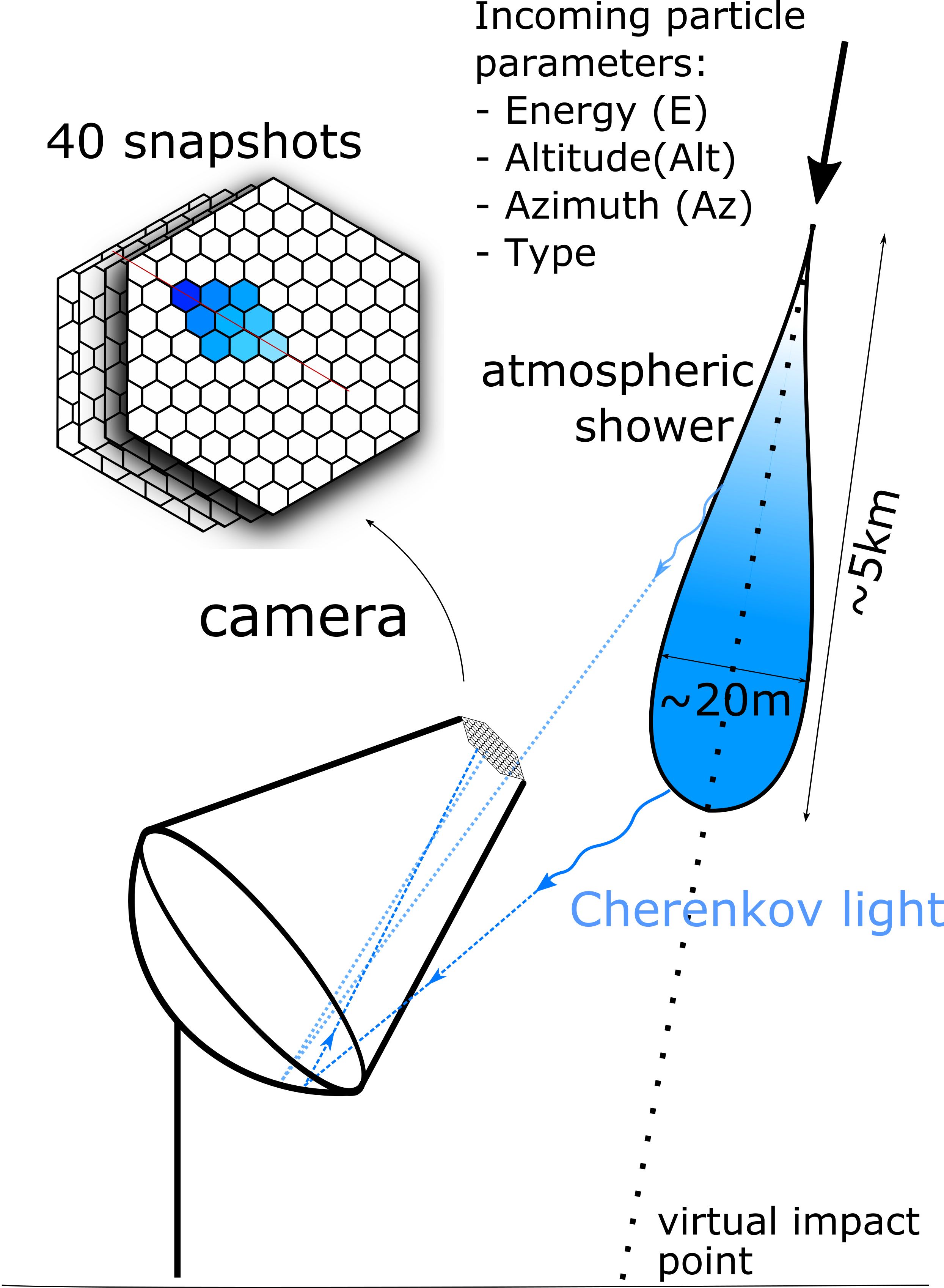
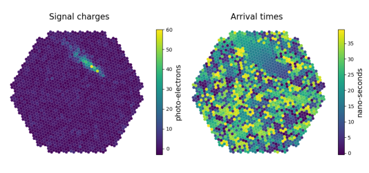
Refer to caption — Figure 1: Top: LST-1 observation principle. Bottom: Extracted signal charges and times.

The Cherenkov light generated by atmospheric showers is collected on the ground by the LST-1 optical system that focuses it to an ultra-fast and sensitive camera sampling the signal into a temporal series of 40 snapshots of 1855 pixels of 1 ns each (also called waveform). This process is depicted in Figure 1. The waveform is then calibrated and integrated to obtain two images, one containing the pixel charges and one the mean arrival time of the Cherenkov photon in each pixel. These two images are then analysed to extract image parameters used to reconstruct the particles physical parameters of interest (type, energy, incoming direction) using machine learning algorithms such as random forests [1].

Thanks to accurate Monte Carlo simulations [2, 3], machine learning algorithms are trained on these images in order to reconstruct the corresponding physical parameters. The algorithms can then be applied to simulated test datasets in order to compute the instrument response function, and so the performance of the reconstruction, or to data from observations.

The steps of image parameters extraction, training, and inference on observations is the one we propose to enhance with deep learning. Indeed, since the AlexNet revolution [4] CNNs have shown in many fields [5] their capacity to replace and overtake solutions with engineered parameters extraction. They have been applied to IACT event reconstruction in the past on CTA simulated data [6, 7, 8] and on H.E.S.S. [9, 10] data, but with limited success on observations. Here we will compare the standard approach using engineered parameters and random forests with the CNN we developed specifically for the tasks at hand, $\gamma$ -PhysNet DA. The first step of calibration plus charge integration is common for both approaches and presented in further details in [11]. It is performed using the lstchain v0.7.3 library [12] based on ctapipe v10.5 [13, 14].

II-A LST-1 classical approach: Hillas and ensemble models

A classical approach, called Hillas by the name of its creator [15], is based on characteristic parameters extracted from these images. This is the standard analysis method in use for LST-1 data analysis. The images first go through a cleaning step called tailcut-cleaning requiring pixels to be above a given picture threshold and a neighbor above a second threshold. The same mask is then applied on the temporal map. Image parameters are then extracted from these cleaned images. The parameters (defined in lstchain v0.7.3) used in this work are: image intensity, ellipsoid width, length, position and orientation in the camera, second order moments, signal time development gradient and charges containment.

Three different random forests (RF) are then trained, one for each task: particle classification, energy reconstruction and direction reconstruction. The performances of these RFs are presented in section III. This approach, later noted Hillas+RF, will serve as the reference for the rest of this work. The complete set of parameters is given in lstchain v0.7.3 standard configuration.

II-B $\gamma$ -PhysNet - a convolutional neural network to analyse LST-1 data

The CNN we developed, $\gamma$ -PhysNet DA, is presented in depth in Ref. [16, 17]. It is a multi-task network, so contrary to the classical approach and to previous works using CNNs, a single algorithm is trained to perform the full event reconstruction (particle classification, energy reconstruction and direction reconstruction). It is composed of a first convolution block common to all tasks and based on ResNet-56 [18] enhanced with indexed convolutions [19] and Dual Attention mechanism [20].

III Performance comparison on simulated data

The Monte Carlo simulations, produced using CORSIKA [2] and simtel_array [3] are fine-tuned to the LST-1 at a pointing of $20\,$ ° zenith in the South direction. The training dataset is composed of isotropic gamma rays and protons while the test dataset is composed of point-source gammas at an offset of 0.4° to the camera center, and isotropic protons and electrons.

Quality cuts are applied to select events: the integrated charge after image cleaning must be greater than 50 photoelectrons, the fraction of that integrated charge in the outermost ring of pixels in the camera must be below 20% and the image must pass a tailcut cleaning with a picture threshold of 6 photoelectrons and a neighbor threshold of 3 photoelectrons. Note however that the cleaning itself is applied only in the case of the Hillas+RF procedure, while the entire image information is kept in the case of $\gamma$ -PhysNet DA.

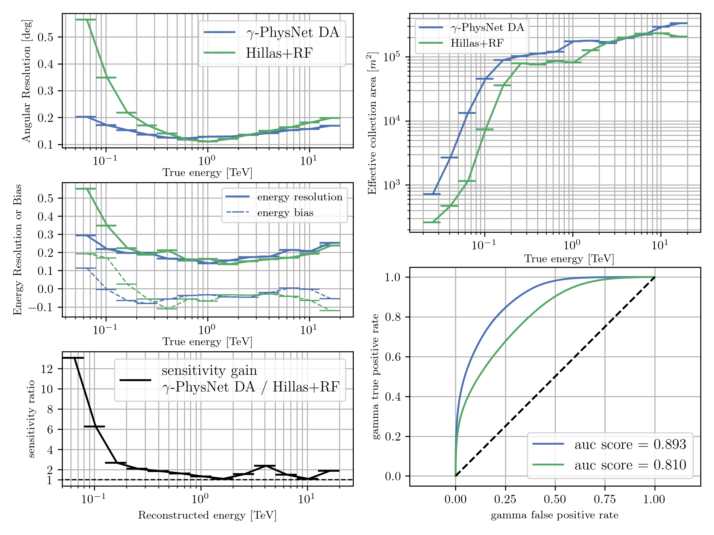
III-A Instrument response functions

Applying the trained algorithms to the test dataset, one can compute the instrument response functions (Figure 2, as defined in Ref. [21]) for the two approaches. The gammaness and angular cuts are determined for best sensitivity in each energy bin using the pyirf v0.4 package [22]. The highest performances of $\gamma$ -PhysNet DA on all tasks are clearly demonstrated at all energies and in particular at the lowest ones (below $300\text{\,}\mathrm{GeV}$ ). The greater classification power of $\gamma$ -PhysNet DA is shown by the higher effective area and by the higher area under the roc curve.

IV Application to LST-1 data

IV-A Methodology

The fairest way to compare the performances of two reconstruction chains is to match their background levels. To do so, we first apply the quality selection cuts common to both chains. Then, we fix the gammaness (likelihood of an event to be a gamma) cut of the standard Hillas+RF analysis at a given level and the gammaness cut of $\gamma$ -PhysNet DA is then determined in order to get the same background level as the one of the reference in each energy bin in the background region (determined with the multiple OFF technique [23]). It is worth noticing that several values have been tested for the reference gammaness cut with no significant change in the results - only one analysis has been kept for simplicity.

IV-B Detection of Markarian 501

Markarian 501 is a well-known blazar at $\text{\,}\mathrm{TeV}$ energy range. The observation dataset is composed of 4 runs taken on the night of the 20 March 2021 for a total of 1h. Observed zenith angles range from 20° to 12.5°. All observations are conducted in wobble mode with an offset of 0.4°.

In this case, the analysis (training and inference) has been performed with cleaning levels of (8,4). The high-level analysis is performed using gammapy v0.18.2 [24], the standard science tool for CTA. Background estimation is done with the reflected multiple off technique [23]. The excess and the background are calculated per reconstructed energy bin.

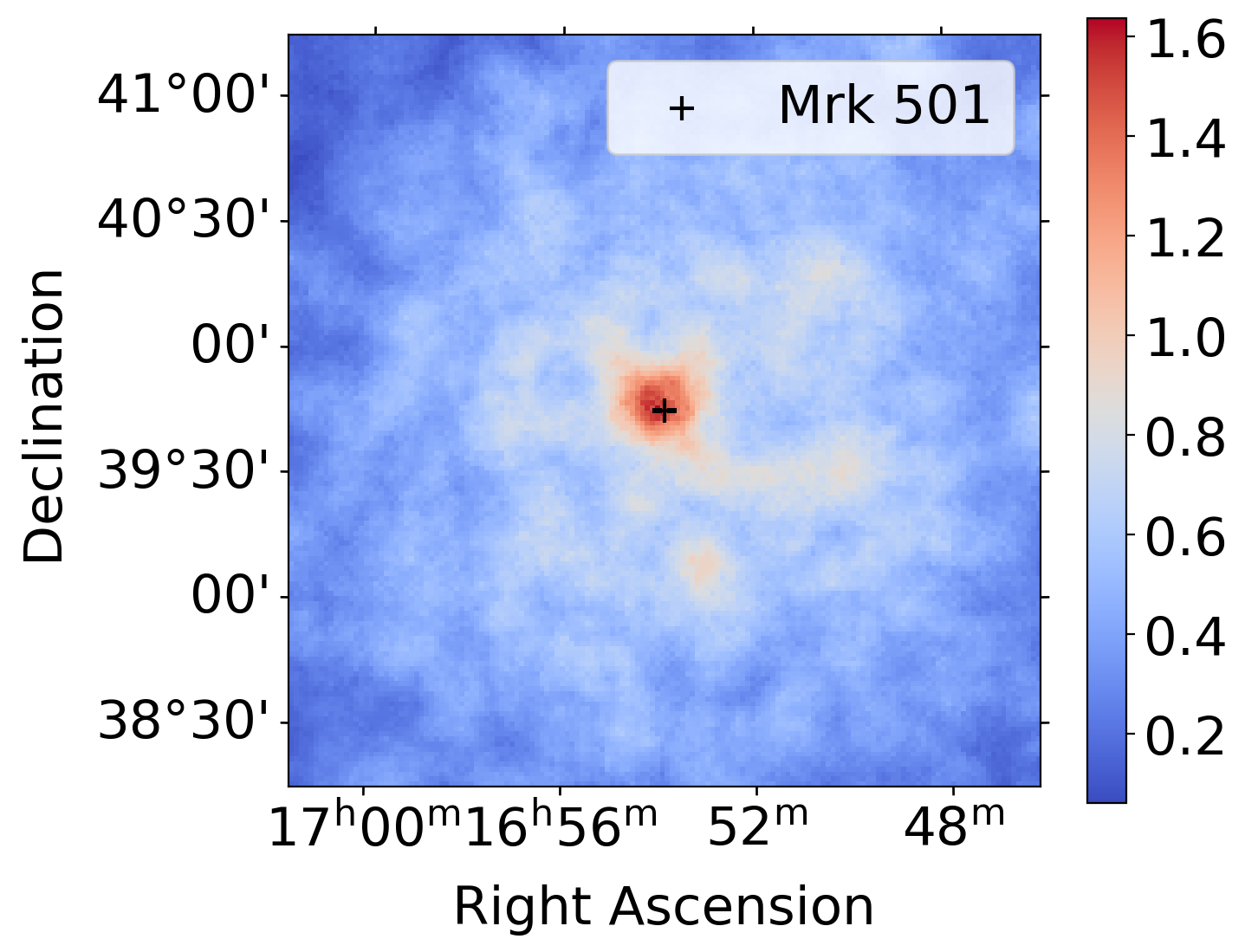
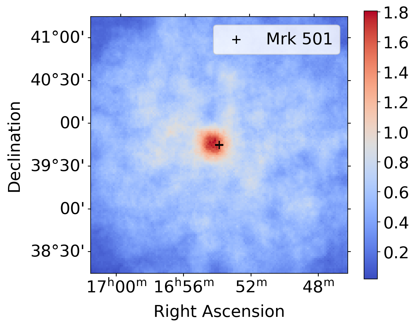
First a counts map of gamma-like events is generated for both chains (Fig. 3). For $\gamma$ -PhysNet DA and Hillas+RF we can notice a hot spot at the source position, later confirmed by proper background estimation and significance calculation. Figure 5 shows the events counts as a function of the separation angle to the source for both chains in OFF and ON regions. On these figures one can observe a bias in the direction reconstruction in the case of $\gamma$ -PhysNet DA. The reason of this bias on observations needs further investigation but preliminary studies show an impact of the discrepancy in pointing direction between simulations and observations. An angular cut of $\theta=0.2\deg$ is applied on data to select the source region in agreement with the average angular resolution and standard cuts applied in LST-1 data analysis [21].

Figure 5 presents a comparative excess count as a function of the reconstructed energy. We can notice the greater excess of gamma-like events detected by $\gamma$ -PhysNet DA compared to the standard Hillas+RF approach, especially at low energies (around $100\text{\,}\mathrm{GeV}$ ). This is in harmony with the results obtained on Monte Carlo simulations presented in figure 2, even though the performance gain is not as large.

Table I provides the integrated counts and significance for both analysis chains. We can notice that the background levels are similar, as imposed by the procedure. We show here that both analysis chains are able to detect Mrk501, with a slight advantage for $\gamma$ -PhysNet DA, showing an integrated excess greater by 30 % ( $\pm 23\%$ ) and a higher significance than the reference.

Reconstruction	Excess	Significance	Background counts
Hillas+RF	148.7 $\gamma$	7.6 $\sigma$	238.3
$\gamma$ -PhysNet DA	192.7 $\gamma$	9.8 $\sigma$	226.3

TABLE I: Excess and significance results for Markarian 501.

IV-C Detection of the Crab Nebula

Here we analyze two observation runs, #2012 (OFF run) and #2013 (ON run) taken in February 2020 at zenith angles of $21.4$ ° and $28.9$ ° respectively. Both runs undergo the same data reduction as described in section III.

The night sky background (NSB) in the Crab Nebula sky region is much higher than in the case of Mrk 501 and more importantly, much higher than the standard NSB used in simulations. As this can negatively impact the analysis, especially in the case of CNNs which are very sensitive to the noise distribution in the images, we add a poissonian noise to the simulated data. Thanks to Raikov’s theorem [25], we determine the parameter of the Poisson distribution as the difference between the simulated average noise pixel charge and the observed one. We can see that the additional noise leads to a better agreement between simulated and observed NSB distributions in figure 6. All models are then retrained with these modified simulations.

Here the standard Hillas+RF (without added noise) serves as a reference for the rest of the analysis and is used for background matching to all others analysis as described in section IV-A.

Figure 8 presents the normalized distributions of the angular separation and figure 8 the excess for all analysis chains. One can see here again the higher excess detected by $\gamma$ -PhysNet DA compared to Hillas+RF, especially at low energies.

Table II displays the final results on Crab Nebula with the excess count, background count and significance. There are several things worth noticing here. First, one can see the higher significance of $\gamma$ -PhysNet DA in its first version (12.5 $\sigma$ ) compared to Hillas+RF (12.0 $\sigma$ ). Then one can see the important improvement brought by the addition of poissonian noise to the simulated dataset, with a final significance of 14.3 $\sigma$ . Finally, one can note the higher robustness of the Hillas+RF analysis, obtaining very similar results (significance of 11.9 $\sigma$ ) after the addition of noise. This is most probably due to the tailcut cleaning applied in this chain which is removing the NSB, thus trading loss of information with robustness.

	Excess	Significance	Background
Hillas+RF	379	$12.0\,\sigma$	308
Hillas+RF	376	$11.9\,\sigma$	305
+ Poisson noise
$\gamma$ -PhysNet DA	395	12.5 $\sigma$	302
$\gamma$ -PhysNet DA	476	14.3 $\sigma$	317
+ Poisson noise

TABLE II: Excess and significance results for Crab Nebula.

V Conclusion

After showing better performances on simulated data, the present study confirms the better sensitivity, especially at low energies, of $\gamma$ -PhysNet DA compared to the classical Hillas+RF reconstruction on observations, with two sources detected with higher significance. The greater gain at low energy can easily be explained by the fact that images are on average noisier at these energies and that convolutional neural networks are more powerful at extracting signal in this case. We also show the importance of closely matching the simulated data with the observed ones taking the NSB as use-case, especially in the case of CNNs which are more sensitive to differences between training and test data. The difference in pointing direction between training data and observation is also expected to play a role and its impact on performances will be studied in a later work. This work shows that CNNs are a valid approach for LST-1 event reconstruction, even though it is still in commissioning phase. As shown, their performances can still be improved by a closer match between simulations and data, which will be further refined by our increased understanding of the telescope. We gratefully acknowledge support from the agencies and organizations listed here: www.cta-observatory.org/consortium_acknowledgment and here: https://gammalearn.pages.in2p3.fr/pages/acknowledgements/.

References

[1] L. Breiman, “Random Forests.” Machine Learning, vol. 45, pp. 5–32, Jan. 2001.
[2] D. Heck et al., “Corsika: A monte carlo code to simulate extensive air showers,” Report fzka, vol. 6019, 1998.
[3] K. Bernlöhr, “Simulation of imaging atmospheric Cherenkov telescopes with CORSIKA and sim_telarray,” Astroparticle Physics, vol. 30, pp. 149–158, 2008.
[4] A. Krizhevsky et al., “Imagenet classification with deep convolutional neural networks,” Commun. ACM, vol. 60, 2017.
[5] J. Gu et al., “Recent Advances in Convolutional Neural Networks,” arXiv e-prints, p. arXiv:1512.07108, Dec. 2015.
[6] D. Nieto Castaño et al., “Exploring deep learning as an event classification method for the Cherenkov Telescope Array,” in 35th ICRC, ser. ICRC, vol. 301, Jan. 2017, p. 809.
[7] D. Nieto Castaño et al., “Reconstruction of iact events using deep learning techniques with ctlearn,” in ADASS XXX, 2020.
[8] M. Jacquemont et al., “Single imaging atmospheric cherenkov telescope full-event reconstruction with a deep multi-task learning architecture,” in ADASS XXX, 2020.
[9] I. Shilon et al., “Application of deep learning methods to analysis of imaging atmospheric cherenkov telescopes data,” Astroparticle Physics, vol. 105, pp. 44–53, 2019.
[10] R. D. Parsons and S. Ohm, “Background rejection in atmospheric Cherenkov telescopes using recurrent convolutional neural networks,” European Physical Journal C, vol. 80, p. 363, May 2020.
[11] Y. t. Kobayashi, “Camera calibration of the cta-lst prototype,” in these proceedings.
[12] R. Lopez-Coto et al. for CTA LST project, “lstchain: An analysis pipeline for LST-1, the first prototype Large-Sized Telescope of CTA,” in ADASS XXX, 2021.
[13] K. Kosack et al., “cta-observatory/ctapipe: v0.10.5,” Mar. 2021.
[14] M. Nöthe et al., “Prototype open event reconstruction pipeline for the cherenkov telescope array,” in these proceedings.
[15] A. Hillas, “Cerenkov light images of eas produced by primary gamma,” in ICRC, vol. 3, 1985.
[16] M. Jacquemont et al., “Multi-task architecture with attention for imaging atmospheric cherenkov telescope data analysis,” in Proceedings of the 16th VISIGRAPP, INSTICC. SciTePress, 2021.
[17] M. Jacquemont et al., “First Full-Event Reconstruction from Imaging Atmospheric Cherenkov Telescope Real Data with Deep Learning,” arXiv e-prints, p. arXiv:2105.14927, May 2021.
[18] K. He et al., “Deep residual learning for image recognition,” in 2016 IEEE Conference on Computer Vision and Pattern Recognition (CVPR), 2016, pp. 770–778.
[19] M. Jacquemont et al., “Indexed operations for non-rectangular lattices applied to convolutional neural networks,” in Proceedings of the 14th VISIGRAPP - Volume 5: VISAPP, INSTICC. SciTePress, 2019, pp. 362–371.
[20] J. Sun et al., “Saunet: Shape attentive u-net for interpretable medical image segmentation,” arXiv preprint arXiv:2001.07645.
[21] O. t. Gueta, “The cherenkov telescope array: layout, design and performances,” in these proceedings, no. 962, 2021.
[22] M. Nöthe et al. (2020, Nov.) pyirf.
[23] Berge, D. et al., “Background modelling in very-high-energy gamma-ray astronomy,” A&A, vol. 466, pp. 1219–1229, 2007.
[24] Nigro, C. et al., “Towards open and reproducible multi-instrument analysis in gamma-ray astronomy,” A&A, vol. 625, p. A10, 2019.
[25] D. Raikov, “On the decomposition of poisson laws,” in Dokl. Akad. Nauk SSSR, vol. 14, no. 1, 1937, pp. 9–12.

Full Authors List: CTA-LST

H. Abe¹, A. Aguasca², I. Agudo³, L. A. Antonelli⁴, C. Aramo⁵, T. Armstrong⁶, M. Artero⁷, K. Asano¹, H. Ashkar⁸, P. Aubert⁹, A. Baktash¹⁰, A. Bamba¹¹, A. Baquero Larriva¹², L. Baroncelli¹³, U. Barres de Almeida¹⁴, J. A. Barrio¹², I. Batkovic¹⁵, J. Becerra González¹⁶, M. I. Bernardos¹⁵, A. Berti¹⁷, N. Biederbeck¹⁸, C. Bigongiari⁴, O. Blanch⁷, G. Bonnoli³, P. Bordas², D. Bose¹⁹, A. Bulgarelli¹³, I. Burelli²⁰, M. Buscemi²¹, M. Cardillo²², S. Caroff⁹, A. Carosi²³, F. Cassol⁶, M. Cerruti², Y. Chai¹⁷, K. Cheng¹, M. Chikawa¹, L. Chytka²⁴, J. L. Contreras¹², J. Cortina²⁵, H. Costantini⁶, M. Dalchenko²³, A. De Angelis¹⁵, M. de Bony de Lavergne⁹, G. Deleglise⁹, C. Delgado²⁵, J. Delgado Mengual²⁶, D. della Volpe²³, D. Depaoli^27,28, F. Di Pierro²⁷, L. Di Venere²⁹, C. Díaz²⁵, R. M. Dominik¹⁸, D. Dominis Prester³⁰, A. Donini⁷, D. Dorner³¹, M. Doro¹⁵, D. Elsässer¹⁸, G. Emery²³, J. Escudero³, A. Fiasson⁹, L. Foffano²³, M. V. Fonseca¹², L. Freixas Coromina²⁵, S. Fukami¹, Y. Fukazawa³², E. Garcia⁹, R. Garcia López¹⁶, N. Giglietto³³, F. Giordano²⁹, P. Gliwny³⁴, N. Godinovic³⁵, D. Green¹⁷, P. Grespan¹⁵, S. Gunji³⁶, J. Hackfeld³⁷, D. Hadasch¹, A. Hahn¹⁷, T. Hassan²⁵, K. Hayashi³⁸, L. Heckmann¹⁷, M. Heller²³, J. Herrera Llorente¹⁶, K. Hirotani¹, D. Hoffmann⁶, D. Horns¹⁰, J. Houles⁶, M. Hrabovsky²⁴, D. Hrupec³⁹, D. Hui¹, M. Hütten¹⁷, T. Inada¹, Y. Inome¹, M. Iori⁴⁰, K. Ishio³⁴, Y. Iwamura¹, M. Jacquemont⁹, I. Jimenez Martinez²⁵, L. Jouvin⁷, J. Jurysek⁴¹, M. Kagaya¹, V. Karas⁴², H. Katagiri⁴³, J. Kataoka⁴⁴, D. Kerszberg⁷, Y. Kobayashi¹, A. Kong¹, H. Kubo⁴⁵, J. Kushida⁴⁶, G. Lamanna⁹, A. Lamastra⁴, T. Le Flour⁹, F. Longo⁴⁷, R. López-Coto¹⁵, M. López-Moya¹², A. López-Oramas¹⁶, P. L. Luque-Escamilla⁴⁸, P. Majumdar^19,1, M. Makariev⁴⁹, D. Mandat⁵⁰, M. Manganaro³⁰, K. Mannheim³¹, M. Mariotti¹⁵, P. Marquez⁷, G. Marsella^21,51, J. Martí⁴⁸, O. Martinez⁵², G. Martínez²⁵, M. Martínez⁷, P. Marusevec⁵³, A. Mas¹², G. Maurin⁹, D. Mazin^1,17, E. Mestre Guillen⁵⁴, S. Micanovic³⁰, D. Miceli⁹, T. Miener¹², J. M. Miranda⁵², L. D. M. Miranda²³, R. Mirzoyan¹⁷, T. Mizuno⁵⁵, E. Molina², T. Montaruli²³, I. Monteiro⁹, A. Moralejo⁷, D. Morcuende¹², E. Moretti⁷, A. Morselli⁵⁶, K. Mrakovcic³⁰, K. Murase¹, A. Nagai²³, T. Nakamori³⁶, L. Nickel¹⁸, D. Nieto¹², M. Nievas¹⁶, K. Nishijima⁴⁶, K. Noda¹, D. Nosek⁵⁷, M. Nöthe¹⁸, S. Nozaki⁴⁵, M. Ohishi¹, Y. Ohtani¹, T. Oka⁴⁵, N. Okazaki¹, A. Okumura^58,59, R. Orito⁶⁰, J. Otero-Santos¹⁶, M. Palatiello²⁰, D. Paneque¹⁷, R. Paoletti⁶¹, J. M. Paredes², L. Pavletić³⁰, M. Pech^50,62, M. Pecimotika³⁰, V. Poireau⁹, M. Polo²⁵, E. Prandini¹⁵, J. Prast⁹, C. Priyadarshi⁷, M. Prouza⁵⁰, R. Rando¹⁵, W. Rhode¹⁸, M. Ribó², V. Rizi⁶³, A. Rugliancich⁶⁴, J. E. Ruiz³, T. Saito¹, S. Sakurai¹, D. A. Sanchez⁹, T. Šarić³⁵, F. G. Saturni⁴, J. Scherpenberg¹⁷, B. Schleicher³¹, J. L. Schubert¹⁸, F. Schussler⁸, T. Schweizer¹⁷, M. Seglar Arroyo⁹, R. C. Shellard¹⁴, J. Sitarek³⁴, V. Sliusar⁴¹, A. Spolon¹⁵, J. Strišković³⁹, M. Strzys¹, Y. Suda³², Y. Sunada⁶⁵, H. Tajima⁵⁸, M. Takahashi¹, H. Takahashi³², J. Takata¹, R. Takeishi¹, P. H. T. Tam¹, S. J. Tanaka⁶⁶, D. Tateishi⁶⁵, L. A. Tejedor¹², P. Temnikov⁴⁹, Y. Terada⁶⁵, T. Terzic³⁰, M. Teshima^17,1, M. Tluczykont¹⁰, F. Tokanai³⁶, D. F. Torres⁵⁴, P. Travnicek⁵⁰, S. Truzzi⁶¹, M. Vacula²⁴, M. Vázquez Acosta¹⁶, V. Verguilov⁴⁹, G. Verna⁶, I. Viale¹⁵, C. F. Vigorito^27,28, V. Vitale⁵⁶, I. Vovk¹, T. Vuillaume⁹, R. Walter⁴¹, M. Will¹⁷, T. Yamamoto⁶⁷, R. Yamazaki⁶⁶, T. Yoshida⁴³, T. Yoshikoshi¹, and D. Zarić³⁵.

¹Institute for Cosmic Ray Research, University of Tokyo. ²Departament de Física Quàntica i Astrofísica, Institut de Ciències del Cosmos, Universitat de Barcelona, IEEC-UB. ³Instituto de Astrofísica de Andalucía-CSIC. ⁴INAF - Osservatorio Astronomico di Roma. ⁵INFN Sezione di Napoli. ⁶Aix Marseille Univ, CNRS/IN2P3, CPPM. ⁷Institut de Fisica d’Altes Energies (IFAE), The Barcelona Institute of Science and Technology. ⁸IRFU, CEA, Université Paris-Saclay. ⁹LAPP, Univ. Grenoble Alpes, Univ. Savoie Mont Blanc, CNRS-IN2P3, Annecy. ¹⁰Universität Hamburg, Institut für Experimentalphysik. ¹¹Graduate School of Science, University of Tokyo. ¹²EMFTEL department and IPARCOS, Universidad Complutense de Madrid. ¹³INAF - Osservatorio di Astrofisica e Scienza dello spazio di Bologna. ¹⁴Centro Brasileiro de Pesquisas Físicas. ¹⁵INFN Sezione di Padova and Università degli Studi di Padova. ¹⁶Instituto de Astrofísica de Canarias and Departamento de Astrofísica, Universidad de La Laguna. ¹⁷Max-Planck-Institut für Physik. ¹⁸Department of Physics, TU Dortmund University. ¹⁹Saha Institute of Nuclear Physics. ²⁰INFN Sezione di Trieste and Università degli Studi di Udine. ²¹INFN Sezione di Catania. ²²INAF - Istituto di Astrofisica e Planetologia Spaziali (IAPS). ²³University of Geneva - Département de physique nucléaire et corpusculaire. ²⁴Palacky University Olomouc, Faculty of Science. ²⁵CIEMAT. ²⁶Port d’Informació Científica. ²⁷INFN Sezione di Torino. ²⁸Dipartimento di Fisica - Universitá degli Studi di Torino. ²⁹INFN Sezione di Bari and Università di Bari. ³⁰University of Rijeka, Department of Physics. ³¹Institute for Theoretical Physics and Astrophysics, Universität Würzburg. ³²Physics Program, Graduate School of Advanced Science and Engineering, Hiroshima University. ³³INFN Sezione di Bari and Politecnico di Bari. ³⁴Faculty of Physics and Applied Informatics, University of Lodz. ³⁵University of Split, FESB. ³⁶Department of Physics, Yamagata University. ³⁷Institut für Theoretische Physik, Lehrstuhl IV: Plasma-Astroteilchenphysik, Ruhr-Universität Bochum. ³⁸Tohoku University, Astronomical Institute. ³⁹Josip Juraj Strossmayer University of Osijek, Department of Physics. ⁴⁰INFN Sezione di Roma La Sapienza. ⁴¹Department of Astronomy, University of Geneva. ⁴²Astronomical Institute of the Czech Academy of Sciences. ⁴³Faculty of Science, Ibaraki University. ⁴⁴Faculty of Science and Engineering, Waseda University. ⁴⁵Division of Physics and Astronomy, Graduate School of Science, Kyoto University. ⁴⁶Department of Physics, Tokai University. ⁴⁷INFN Sezione di Trieste and Università degli Studi di Trieste. ⁴⁸Escuela Politécnica Superior de Jaén, Universidad de Jaén. ⁴⁹Institute for Nuclear Research and Nuclear Energy, Bulgarian Academy of Sciences. ⁵⁰FZU - Institute of Physics of the Czech Academy of Sciences. ⁵¹Dipartimento di Fisica e Chimica ’E. Segrè’ Università degli Studi di Palermo. ⁵²Grupo de Electronica, Universidad Complutense de Madrid. ⁵³Department of Applied Physics, University of Zagreb. ⁵⁴Institute of Space Sciences (ICE-CSIC), and Institut d’Estudis Espacials de Catalunya (IEEC), and Institució Catalana de Recerca I Estudis Avançats (ICREA). ⁵⁵Hiroshima Astrophysical Science Center, Hiroshima University. ⁵⁶INFN Sezione di Roma Tor Vergata. ⁵⁷Charles University, Institute of Particle and Nuclear Physics. ⁵⁸Institute for Space-Earth Environmental Research, Nagoya University. ⁵⁹Kobayashi-Maskawa Institute (KMI) for the Origin of Particles and the Universe, Nagoya University. ⁶⁰Graduate School of Technology, Industrial and Social Sciences, Tokushima University. ⁶¹INFN and Università degli Studi di Siena, Dipartimento di Scienze Fisiche, della Terra e dell’Ambiente (DSFTA). ⁶²Palacky University Olomouc, Faculty of Science. ⁶³INFN Dipartimento di Scienze Fisiche e Chimiche - Università degli Studi dell’Aquila and Gran Sasso Science Institute. ⁶⁴INFN Sezione di Pisa. ⁶⁵Graduate School of Science and Engineering, Saitama University. ⁶⁶Department of Physical Sciences, Aoyama Gakuin University. ⁶⁷Department of Physics, Konan University.